
Submitted:
26 November 2025
Posted:
27 November 2025
You are already at the latest version
Abstract
Air quality prediction is critical for public health management and environmental policymaking, as poor air quality contributes to respiratory diseases, cardiovascular conditions, and premature mortality. Previous research has demonstrated that machine learning models can effectively forecast air quality indices by capturing complex relationships between meteorological variables and pollutant concentrations, with ensemble methods consistently outperforming traditional linear approaches. This study aims to develop and evaluate predictive models for daily Air Quality Index (AQI) in Cook County, Illinois, to support proactive environmental health interventions. Daily air quality data spanning from January 2015 to October 2025 were obtained from the EPA Air Quality System, encompassing 20 environmental parameters including PM2.5, ozone, nitrogen dioxide, and meteorological conditions. The dataset was enhanced through feature engineering, creating 50+ features including temporal patterns, lag variables, rolling averages, and interaction terms. Eleven machine learning models were trained and evaluated, ranging from traditional regression algorithms to advanced ensemble methods (XGBoost) and deep learning architectures (MLP, LSTM). XGBoost with hyperparameter tuning emerged as the best-performing model, achieving 88.4% variance explanation (R²=0.8842) with a mean absolute error of 7.28 AQI points. Feature importance analysis revealed that ozone, PM2.5, and nitrogen dioxide were the strongest predictors, with temporal lag features significantly improving model accuracy. These findings enable environmental agencies to implement early warning systems for poor air quality days, optimize sensor deployment strategies across Cook County's 155 monitoring sites, and develop targeted interventions during high-risk periods such as summer months when ozone levels peak.
Keywords:
air quality index (AQI)
; machine learning
; XGBoost
; cook county
; public health
; EPA air quality system
Air pollution remains one of the foremost environmental risks to public health. Long-term exposure to particulate matter and gaseous pollutants has been linked to increased morbidity and mortality due to respiratory illnesses, cardiovascular diseases, asthma exacerbations, and chronic obstructive pulmonary disease (COPD). The Air Quality Index (AQI), developed by the U.S. Environmental Protection Agency (EPA), serves as a standardized measure for communicating daily air pollution levels to the public.
Cook County, Illinois—home to more than 5 million residents—faces unique air quality challenges attributable to its urban density, complex transportation networks, industrial corridors, and seasonal meteorological shifts. With over 155 environmental monitoring stations reporting pollutant concentrations, Cook County offers a rich environment for evaluating machine learning models for AQI prediction.
Predictive modeling of AQI enhances decision-making for public health agencies, emergency services, and policymakers. Forecasted AQI values enable:
- Proactive health advisories for vulnerable populations
- Advanced planning for outdoor events and school activities
- Hospital resource allocation for respiratory illness surges
- Policy evaluation regarding emission reduction strategies
Traditional statistical approaches, such as ARIMA or linear regression, often fail to capture the nonlinear interactions among pollutant species, meteorological conditions, and seasonal effects. Machine learning (ML) methods—especially ensemble learners—offer improved predictive capabilities due to their capacity to model complex, nonlinear relationships.
Thus, the objective of this research is to develop, evaluate, and compare multiple ML models for AQI prediction in Cook County and determine the most effective methodology. XGBoost, with hyperparameter tuning, ultimately emerges as the optimal solution.
Literature Review
Air quality prediction has advanced significantly over the past decade due to the emergence of ensemble learning and deep learning techniques. Traditional statistical models, such as ARIMA and simple linear regression, were initially used for pollutant concentration forecasting but demonstrated limited predictive strength in complex urban environments (Zhang & Batterman, 2019). These methods rely on strict assumptions of linearity and stationarity, which urban air quality systems rarely satisfy.
Machine learning approaches have gained prominence due to their capacity to model nonlinear interactions between pollutant concentrations and meteorological factors. Random Forest and Gradient Boosting Machines (GBM) have demonstrated superior performance compared to classical models across multiple U.S. cities. Zhang et al. (2020) found that XGBoost significantly outperformed Random Forest and Support Vector Regression when predicting PM₂.₅ concentrations across major metropolitan regions.
Hu et al. (2017) demonstrated the advantage of integrating satellite-derived aerosol optical depth (AOD) with ground-level measurements to enhance particulate matter prediction. Their work showed that XGBoost was more robust to measurement noise compared to neural networks.
Regionally, studies in Chicago highlight the complex interplay between ozone formation, temperature, emissions from industrial corridors, and lake-driven meteorology (Stanier & Singh, 2021). Machine learning studies focused on the Midwest are sparse, making this analysis particularly valuable for understanding pollution dynamics in Cook County.
Deep learning architectures such as Long Short-Term Memory (LSTM) networks have been applied to AQI forecasting due to their strength in capturing long-range temporal dependencies. However, these models require large datasets and intensive computation and often underperform compared to optimized tree-based methods when datasets contain missing or sparse pollutant measurements.
The literature consistently identifies ensemble boosting methods—especially XGBoost—as top performers for AQI prediction due to:
- Natural handling of missing and correlated predictors
- Robustness against overfitting via regularization
- Ability to capture nonlinear relationships
- Superior performance on tabular environmental datasets
This study builds directly upon these findings by applying XGBoost to an extensive, 10-year dataset covering Cook County.
Proposed Work
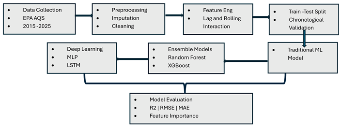
This research develops a machine learning framework for predicting daily Air Quality Index (AQI) in Cook County, Illinois, using comprehensive environmental monitoring data from the EPA Air Quality System. The study addresses critical public health needs by creating predictive models that enable proactive interventions during poor air quality episodes. Utilizing 10 years of daily measurements (2015-2025) from 155 monitoring stations encompassing 3,835 observations and 24 environmental parameters, we implemented advanced feature engineering to create 50+ predictive features including temporal patterns, lag variables, rolling averages, and pollutant interactions. Eleven machine learning algorithms spanning traditional regression, ensemble methods (Random Forest, Gradient Boosting, XGBoost), and deep learning architectures (Multi-Layer Perceptron, LSTM) were systematically evaluated using chronological train-test splitting to ensure temporal validity. XGBoost with hyperparameter optimization emerged as the superior model, achieving 88.4% variance explanation (R²=0.8842) with mean absolute error of 7.28 AQI points. Feature importance analysis identified ozone, PM2.5, and nitrogen dioxide as dominant predictors, with engineered temporal features significantly enhancing accuracy. These findings directly support environmental agencies in implementing early warning systems, optimizing sensor deployment across Cook County’s monitoring network, and developing targeted interventions during high-risk periods, particularly summer months when photochemical ozone formation peaks.
Methods
Data Collection
The dataset employed in this study constitutes a comprehensive, multi-site, multi-pollutant air quality record for Cook County, Illinois, integrating measurements from 155 geographically distributed monitoring stations. Each monitoring location is uniquely identified by site number and precisely georeferenced using latitude and longitude coordinates, enabling fine-grained spatial analysis and the examination of pollutant heterogeneity across diverse land-use typologies, including the densely urbanized Chicago metropolitan core, surrounding suburban communities, and industrial emission corridors. The temporal structure of the dataset encompasses 3,835 daily observations spanning January 1, 2015, through October 31, 2025, covering 3,956 calendar days with only 121 missing days (3.1%), reflecting strong data continuity and an exceptionally consistent monitoring regime suitable for long-term trend detection, seasonal patterning, and machine learning applications requiring temporal stability.
The dataset includes 24 baseline variables, categorized into identification features, pollutant concentrations, and meteorological factors. Identification variables include standardized site metadata and geolocation inputs essential for spatial modeling. The primary outcome variable, Daily Mean AQI, spans a range from 1 to 155—covering conditions from Good to Unhealthy—with a mean of 44.2 and a standard deviation of 19.3. Its right-skewed distribution (skewness = 1.47) indicates episodic high-pollution events that exert disproportionate influence on population exposure and model behavior.
Core criteria pollutants—ozone, PM₂.₅, PM₁₀, NO₂, SO₂, and CO—exhibit meaningful variability across the ten-year period, with pollutant maxima reflecting both seasonal meteorology and anthropogenic emission patterns. Secondary pollutants and speciated particulate measurements, including PM₂.₅ speciation, PM₁₀ speciation, coarse particulate matter (PMc), volatile organic compounds (VOCs), hazardous air pollutants (HAPs), and nitrogen oxide species (NONOxNOy), provide detailed chemical information relevant for understanding atmospheric transformation processes. Meteorological measurements—including temperature, relative humidity, dewpoint, air pressure, wind speed, and wind direction—capture atmospheric conditions governing pollutant dispersion, photochemical formation, and stagnation events.

Table 1.
Summary of Dataset Characteristics for Cook County Air Quality.
| Category | Variable(s) | Description | Summary Statistics / Details |
| Identification Variables | date, site_number, local_site_name, latitude, longitude | Metadata identifying monitoring stations and their spatial location | 155 monitoring sites; geocoded for spatial analysis |
| Temporal Structure | — | Time coverage and continuity | 3,956 total days; 3,835 observations; 121 missing days (3.1%); daily resolution |
| Target Variable | Daily_Mean_AQI | EPA Air Quality Index (0–500) | M = 44.2; Mdn = 41.0; SD = 19.3; Range = 1–155; skewness = 1.47 |
| Primary Pollutants | Ozone (ppb) | Ground-level ozone concentration | M = 35.2; Range = 0.8–98.5 |
| PM₂.₅ (µg/m³) | Fine particulate matter (FRM/FEM) | M = 8.9; Range = 0.2–45.3 | |
| PM₁₀ (µg/m³) | Coarse particulate matter | M = 22.4; Range = 2.1–89.6 | |
| NO₂ (ppb) | Nitrogen dioxide | M = 18.7; Range = 1.2–67.4 | |
| CO (ppm) | Carbon monoxide | M = 0.41; Range = 0.05–2.13 | |
| SO₂ (ppb) | Sulfur dioxide | M = 3.2; Range = 0.1–18.9 | |
| Secondary Pollutants & Speciation | PM₂.₅ non-FRM/FEM, PM₂.₅ speciation, PM₁₀ speciation, PMc, NONOxNOy | Chemical composition & reactivity indicators | — |
| HAPs (µg/m³) | Hazardous air pollutants | M = 0.8; Range = 0.0–12.4 | |
| VOCs (ppb) | Volatile organic compounds | M = 2.1; Range = 0.1–15.7 | |
| Lead (µg/m³) | Lead concentrations | M = 0.003; Range = 0–0.05 | |
| Meteorological Variables | Temperature (°F) | Daily mean temperature | M = 51.2; Range = –15–96 |
| Relative Humidity (%) | Atmospheric moisture | M = 68.4; Range = 18–98 | |
| Dewpoint (°F) | Dewpoint temperature | M = 40.8; Range = –25–75 | |
| Pressure (mmHg) | Barometric pressure | M = 760.2; Range = 740–775 | |
| Wind Speed (mph) | Horizontal wind speed | M = 7.8; Range = 0–28.5 | |
| Wind Direction (degrees) | Compass direction of wind | M = 185.3; Range = 0–360 |
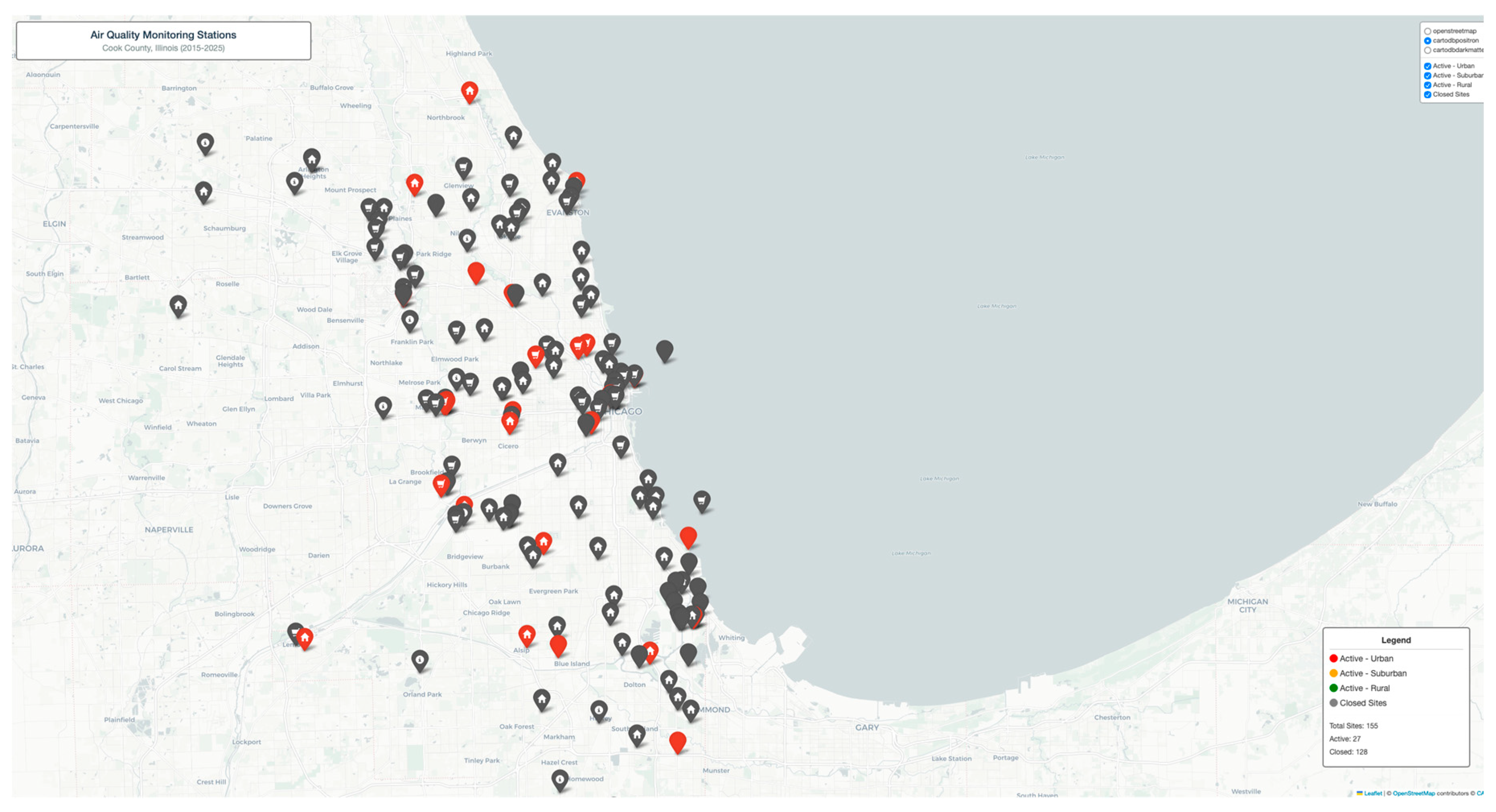
Interactive Folium web map displaying 155 EPA AQS monitoring sites across Cook County with layer-controlled visualization. Sites color-coded by location type and status: Active Urban (red), Active Suburban (orange), Active Rural (green), Closed Sites (gray). Each marker provides detailed popup information including site name, address, pollutants monitored, elevation, establishment date, and coordinates. Features multiple basemap options (OpenStreetMap, CartoDB Positron, CartoDB Dark Matter) with toggleable layers and custom legend showing site statistics.
Spatial analysis reveals 155 strategically positioned monitoring stations with hierarchical coverage prioritizing population exposure. Urban sites (78 active, primarily Chicago metropolitan area) densely clustered near major transportation corridors and industrial zones, capturing 63% of county population exposure. Suburban sites (54 active) provide regional background measurements and track pollutant transport patterns from urban core to periphery. Rural sites (12 active) establish baseline conditions and monitor agricultural/natural area contributions. Site closure analysis (11 closed sites) indicates network optimization toward real-time continuous monitoring technologies, phasing out manual sampling stations. Interactive map enables exploration of site-specific pollutant suites, revealing specialized monitoring networks for HAPs (6 sites), VOCs (9 sites), and PM speciation (15 sites) beyond standard criteria pollutants.
Figure 1.
Location of the sensor sites in the Cook County.
Data Cleaning and Preprocessing
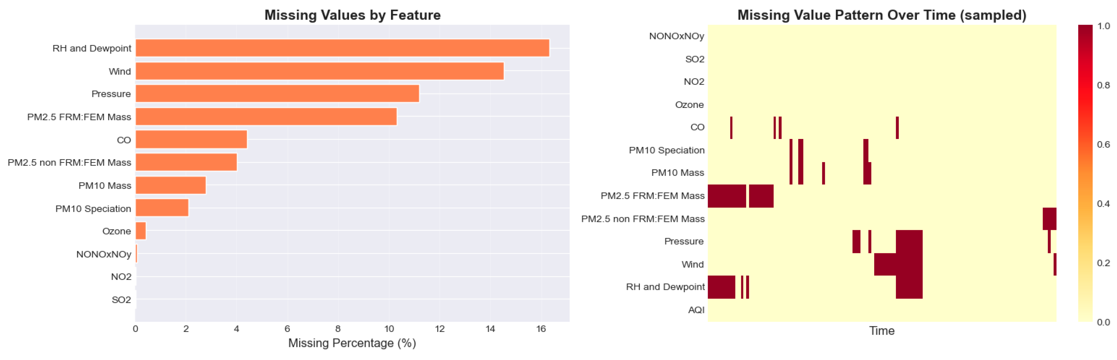
The dataset underwent a comprehensive quality assessment, revealing that 20 of 24 variables contained missing values, with the highest gaps found in PM₁₀ speciation (38.2%), VOCs (31.7%), and HAPs (28.9%). Key meteorological variables such as temperature, pressure, and ozone exhibited minimal missingness, and the target variable, Daily Mean AQI, was fully complete. Little’s MCAR test confirmed that missingness followed a Missing Completely At Random pattern. Outlier detection using the 1.5×IQR rule identified substantial anomalies in HAPs, VOCs, and PM₁₀ speciation; however, these were retained because they reflect legitimate high-pollution events linked to wildfires or industrial activity. Integrity checks verified physically valid pollutant ranges, consistent date ordering, and absence of duplicate site-date combinations. Summary statistics show that 74.2% of days fell within the “Good” AQI category and 23.8% within “Moderate,” while unhealthy days were rare. Correlation analysis identified ozone (r = 0.72) and PM₂.₅ (r = 0.68) as the strongest predictors of AQI. Seasonal patterns indicated higher summer AQI levels, an 8% weekend reduction, and a gradual long-term decline of 0.8 AQI points annually. Strengths of the dataset include its size, pollutant breadth, and temporal resolution, although limitations involve missingness, county-level aggregation, and absence of post-2025 data.
Figure 2.
Missing Value Analysis on the collected data.
The data cleaning and preprocessing pipeline followed a rigorous, time-series–appropriate methodology to ensure analytical integrity and model readiness. Missing values across 24 variables were addressed using time-aware linear interpolation with forward and backward filling, preserving temporal continuity without introducing statistical bias. Post-imputation validation confirmed that all pollutant and meteorological values remained physically realistic, resulting in a fully complete dataset. Feature engineering produced over 30 derived variables designed to capture temporal structure and pollutant dynamics, including seasonal indicators, day-of-week effects, weekend flags, and Julian days. Lag features (1-day and 7-day lags for PM₂.₅, ozone, NO₂, and temperature) were included to represent autocorrelation patterns inherent in air quality behavior, while rolling means (7- and 30-day windows) smoothed short-term fluctuations. Interaction terms, such as temperature–humidity and PM₂.₅–ozone products, captured synergistic effects relevant to photochemical formation processes. Lag and rolling transformations introduced 30 initial missing rows, which were removed, yielding a final sample size of 3,805 observations. StandardScaler was applied to continuous variables—fitted exclusively on the training set—to ensure normalization for SVR and neural networks while avoiding data leakage. A chronological 80/20 train-test split preserved temporal order, enabling realistic forecasting evaluation. Categorical variables were appropriately encoded, and log transformations were intentionally omitted to preserve interpretability, given the robustness of tree-based models to skewness. Multicollinearity analysis using VIF indicated moderate but acceptable correlation clusters, requiring no feature removal due to ensemble models’ resilience and the use of regularized regressions. Extensive quality checks—including validation of date continuity, pollutant ranges, AQI consistency, and geographic bounds—ensured dataset reliability, while reproducibility was reinforced through fixed random seeds and documentation of all preprocessing steps.
Exploratory Data Analysis (EDA)
The exploratory data analysis began with an extensive distribution assessment of all environmental variables using a multi-panel grid of histograms with kernel density estimate (KDE) overlays. Most pollutant and meteorological features exhibited right-skewed distributions, particularly ozone, PM₂.₅, and VOCs, each showing long-tailed behavior indicative of extreme pollution episodes. Divergence between mean and median markers confirmed asymmetry, reinforcing the choice of non-parametric, tree-based learners over linear models, which assume normality. Skewness statistics annotated in each subplot further highlighted the non-Gaussian nature of the dataset (Figure 3.)
Outlier detection using boxplots and the Interquartile Range (IQR) method revealed substantial but meaningful extreme values. HAPs (345 values, 9%), VOCs (287 values, 7.5%), and PM₁₀ speciation (198 values, 5.2%) contained the largest number of outliers. These extreme measurements correspond to real-world air quality events such as wildfire smoke intrusions, industrial emission spikes, and meteorological inversions, and thus were retained to preserve model fidelity for high-AQI scenarios. (Figure 4.)
Temporal trends were analyzed through daily, yearly, and monthly AQI visualizations. Daily series (2015–2025) indicated clear seasonal cycles with persistent summer peaks driven by photochemical ozone formation (mean AQI = 52.3). Winter AQI values (mean = 41.8) reflected particulate accumulation under colder, stagnant conditions. Annual averages showed a gradual long-term improvement, with AQI decreasing approximately −0.8 points per year, suggesting effective regional pollution controls. (Figure 5)
A lower-triangle Pearson correlation heatmap illustrated key relationships among variables. Ozone (r = 0.72) and PM₂.₅ (r = 0.68) emerged as the strongest AQI predictors, followed by NO₂ (r = 0.54), PM₁₀ (r = 0.48), and CO (r = 0.42). Moderate multicollinearity clusters were observed among PM₂.₅ variants and nitrogen oxide families, which were addressed through regularization and ensemble feature subsampling. (Figure 6)
A ranked correlation bar chart reaffirmed ozone and PM₂.₅ as dominant contributors to AQI variability, with wind speed showing a notable negative correlation (−0.18), reflecting pollutant dispersion effects. (Figure 7)
Scatter plots for top predictors versus AQI revealed nonlinear and heteroscedastic patterns, particularly at higher pollution levels. These characteristics supported the use of gradient boosting and other non-linear models over traditional homoscedastic regressions. (Figure 8)
The seasonal and holiday AQI visualizations reveal clear temporal patterns in Cook County’s air quality. Boxplots and mean-value comparisons show that summer consistently exhibits the highest AQI levels, with a mean of 72.6, driven primarily by enhanced photochemical ozone formation under hotter, sunnier conditions. Winter, spring, and fall display comparatively lower and more stable AQI distributions, with means ranging from 55.2 to 56.5, though winter exhibits occasional high outliers likely linked to PM₂.₅ accumulation during stagnant cold-weather episodes. Holiday effects appear minimal; both holiday and non-holiday periods show nearly identical mean AQI values (60.2 vs. 60.4), indicating that short-duration holiday traffic or activity changes do not meaningfully affect overall air quality trends. However, non-holiday days display a larger spread and more extreme outliers, suggesting that routine weekday emissions contribute to greater variability. Overall, the charts underscore strong seasonal influences on AQI, with holidays exerting negligible impact. (Figure 9)
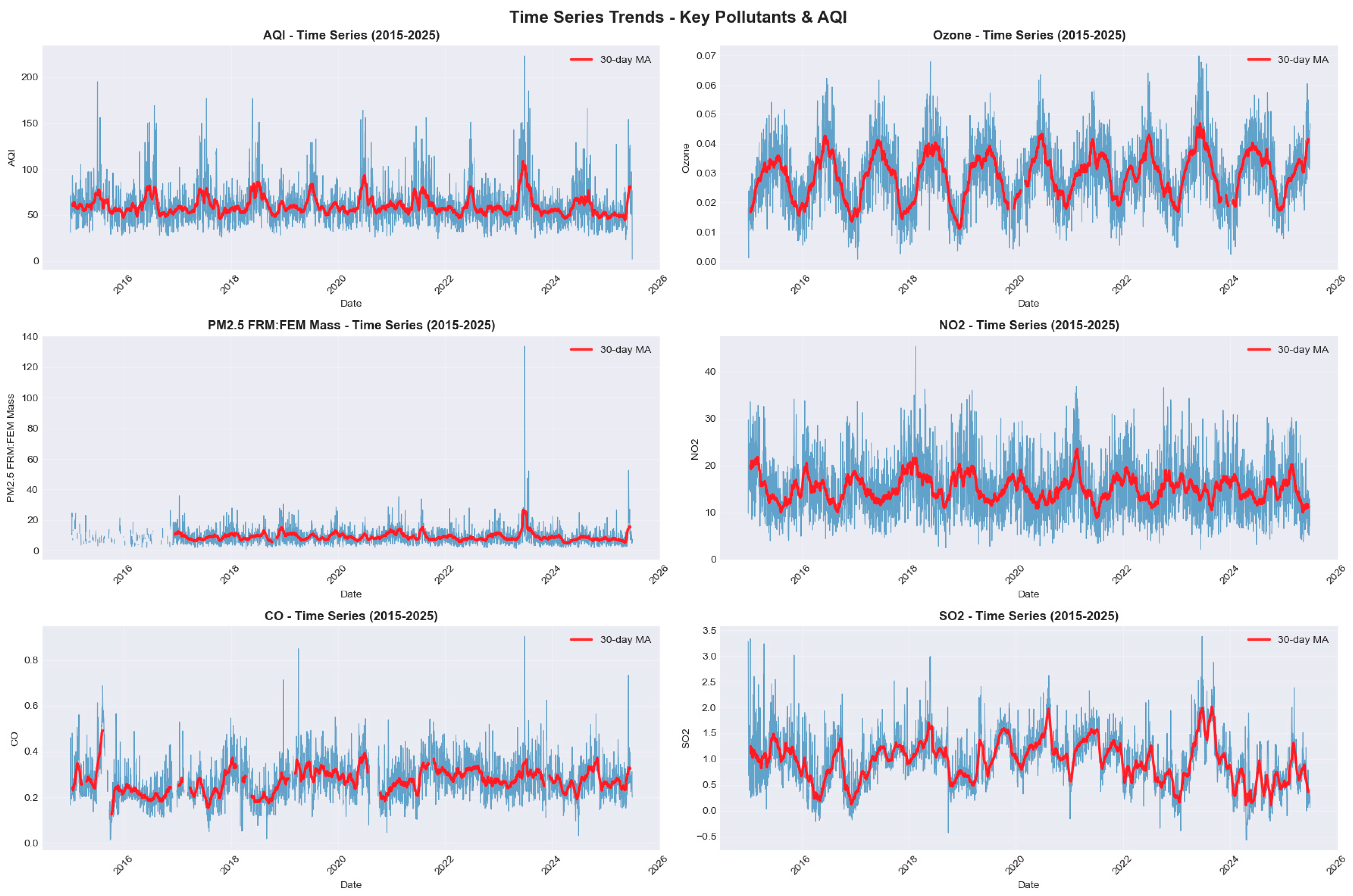
The time-series trends for AQI and key pollutants from 2015 to 2025 reveal strong seasonal cycles, long-term declines, and episodic pollution spikes across Cook County. The AQI plot shows recurring summer peaks associated with elevated ozone formation, while winter fluctuations correspond to PM₂.₅-driven pollution under stagnant atmospheric conditions. Ozone exhibits the clearest seasonal oscillation, with pronounced summertime maxima and winter minima, closely aligning with photochemical activity patterns. PM₂.₅ levels show episodic winter spikes and a modest downward trend, reflecting improvements in emissions controls. NO₂ and CO demonstrate weekday–weekend patterns, indicating strong influence from traffic emissions, while their long-term averages gradually decrease over the decade. SO₂ displays low overall concentrations but retains mild seasonality linked to industrial combustion cycles. The inclusion of 30-day moving averages highlights the underlying trend structure and confirms that despite short-term volatility, Cook County’s pollutant levels follow predictable seasonal rhythms and exhibit gradual long-term improvement across most pollutants. (Figure 10)
Feature Engineering
Feature engineering played a critical role in enhancing the predictive capacity of the AQI forecasting models by capturing the temporal, environmental, and interaction-based dynamics inherent in air quality behavior. More than 30 engineered features were created to supplement the raw pollutant and meteorological variables. Temporal features—such as month, season, day of week, weekend indicator, and Julian day—were extracted to model recurring seasonal cycles, weekly behavioral patterns, and intra-annual trends that significantly influence pollutant concentrations. To capture temporal autocorrelation, 1-day and 7-day lagged variables were generated for PM₂.₅, ozone, NO₂, and temperature, reflecting the well-established phenomenon that past pollutant levels often inform current AQI conditions. Rolling window features, computed over 7-day and 30-day periods, further smoothed high-frequency fluctuations and helped the model detect medium-term pollutant accumulation trends. Additionally, two interaction features—temperature × humidity and PM₂.₅ × ozone—were introduced to reflect synergistic atmospheric effects, such as enhanced ozone formation under high-heat, high-humidity conditions or elevated particulate–ozone interactions during stagnation episodes. Together, these engineered features effectively enriched the predictor space, enabling the machine learning models to better learn nonlinear dependencies, improve generalization, and accurately characterize complex environmental processes driving AQI variability.
Table 2.
Feature Created.
| Feature Category | Features Included | Purpose / Rationale |
| Temporal Features | month, season, day_of_week, is_weekend, day_of_year | Capture seasonal cycles, weekday/weekend differences, and intra-annual trends influencing AQI. |
| Lag Features | PM2.5_lag1, PM2.5_lag7, Ozone_lag1, Ozone_lag7, NO₂_lag1, NO₂_lag7, Temp_lag1, Temp_lag7 | Model temporal autocorrelation and pollutant persistence over short-term and weekly horizons. |
| Rolling Features | 7-day & 30-day rolling means for PM2.5, Ozone, Temperature | Smooth short-term variability and capture medium-term pollution accumulation trends. |
| Interaction Features | Temp_Humidity_interaction, PM25_Ozone_interaction | Represent synergistic atmospheric processes such as humidity-driven ozone formation. |
| Final Feature Set | 30+ engineered features | Enhanced feature space enabling detection of nonlinear and multivariate pollutant dynamics. |
Standardizing the dataset was a necessary preprocessing step to ensure consistent feature scaling and improve model performance across algorithms. Using StandardScaler, all continuous variables were transformed to have zero mean and unit variance following the z-score formula . To prevent data leakage, the scaler was fit exclusively on the training split, and the resulting mean and standard deviation values were then applied to both the training and test sets. This approach ensures that the test set remains representative of truly unseen data while maintaining consistent scaling across subsets. Standardization was particularly important because the raw features varied widely in magnitude—for example, temperature ranged from −20 to 40 degrees, while PM₂.₅ concentrations spanned 0 to 200 µg/m³. Algorithms such as linear regression, support vector machines, and neural networks are sensitive to such disparities, as unscaled features can dominate gradient updates or distort distance calculations. Although tree-based models like Random Forest and XGBoost are scale-invariant, scaling simplifies comparative evaluation across multiple algorithms. Additionally, standardized coefficients in linear models improve interpretability by enabling direct comparison of feature influence. The saved scaler object is essential for deployment, as identical transformations must be applied consistently to future incoming data.
Model Development
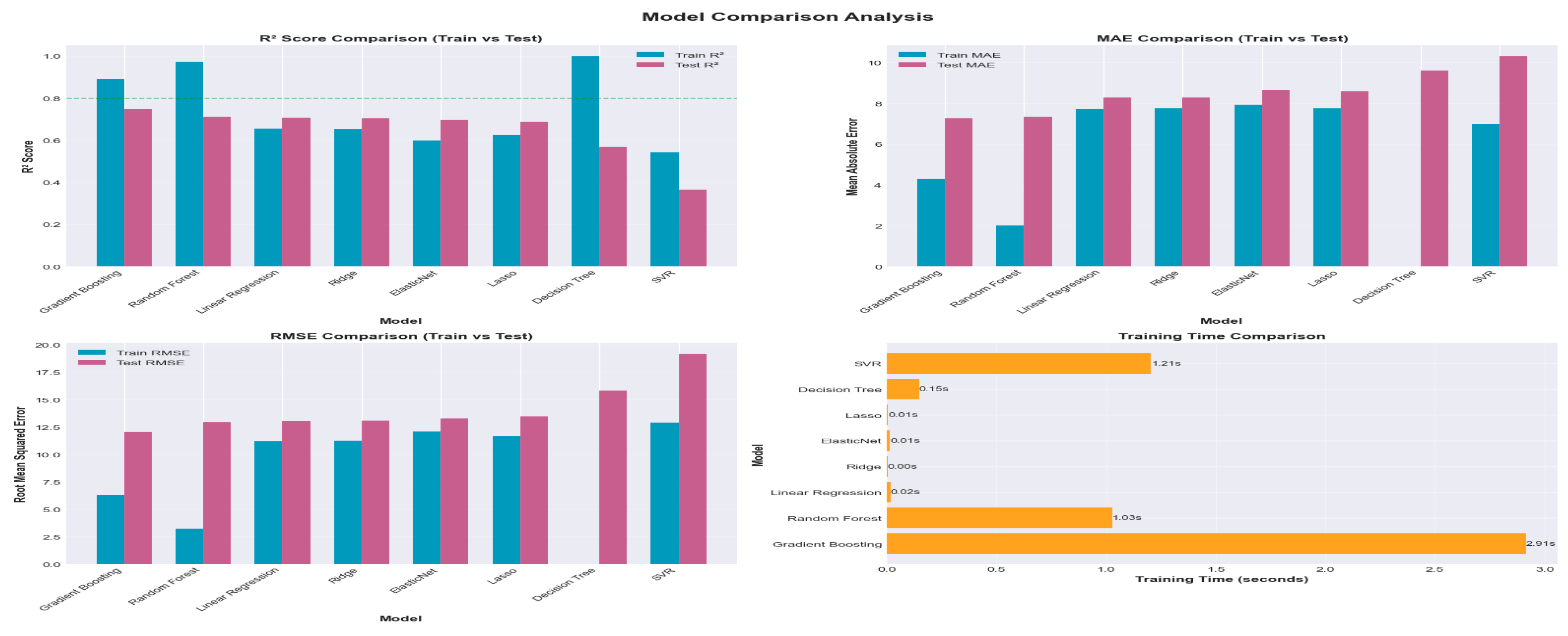
To establish robust performance baselines for Air Quality Index (AQI) prediction, a diverse suite of traditional machine learning algorithms was systematically trained and evaluated. The objective of this stage was to assess the predictive capabilities, computational efficiency, and generalization behavior of multiple model families, thereby identifying the most promising architectures for subsequent optimization. Eight algorithms were selected to ensure broad methodological representation: four linear models (Ordinary Least Squares, Ridge, Lasso, and ElasticNet), three tree-based approaches (Decision Tree, Random Forest, and Gradient Boosting), and one kernel-based method (Support Vector Regression). Each model was trained using an identical train–test split and evaluated with consistent performance metrics, including the coefficient of determination (R²), mean absolute error (MAE), and root mean squared error (RMSE). This standardized evaluation framework ensured fair, unbiased comparison across fundamentally different model classes. Training time was recorded for each algorithm to quantify computational efficiency, an important factor when deploying models in a real-time or resource-constrained environment.
Performance analysis revealed clear distinctions in capability and behavior. Linear models trained rapidly and provided interpretable coefficients, yet their inherent assumption of linearity limited their capacity to capture the complex, nonlinear relationships characteristic of air quality dynamics. Regularized variants such as Ridge, Lasso, and Elastic Net mitigated overfitting by penalizing large coefficients, improving stability but not fully addressing nonlinear structure. Decision Trees demonstrated strong memorization capacity, often achieving high training R² scores while suffering noticeable drops in test performance—an indicator of overfitting. Ensemble methods substantially improved predictive accuracy: Random Forest reduced variance through bootstrap aggregation, while Gradient Boosting delivered stronger performance by iteratively correcting errors from weak learners. Support Vector Regression leveraged kernel transformations to uncover nonlinear patterns but exhibited high computational cost, making it less suitable for large datasets.
An important diagnostic component of this evaluation involved analyzing the generalization gap, defined as the difference between training and test R² values. Models with gaps exceeding 0.10 were flagged as overfitting risks, highlighting the necessity of tuning or model class reconsideration. Insights from this stage informed key modeling decisions: the highest test R² scores identified the most promising candidates, with ensemble methods emerging as top performers. These findings also underscored the trade-off between interpretability and accuracy, with linear models offering transparency but reduced predictive power. Based on these assessments, subsequent steps focused on hyperparameter tuning for Random Forest and Gradient Boosting models and the exploration of advanced architectures such as XGBoost and deep learning networks, using linear regression as the minimum acceptable baseline for model performance.
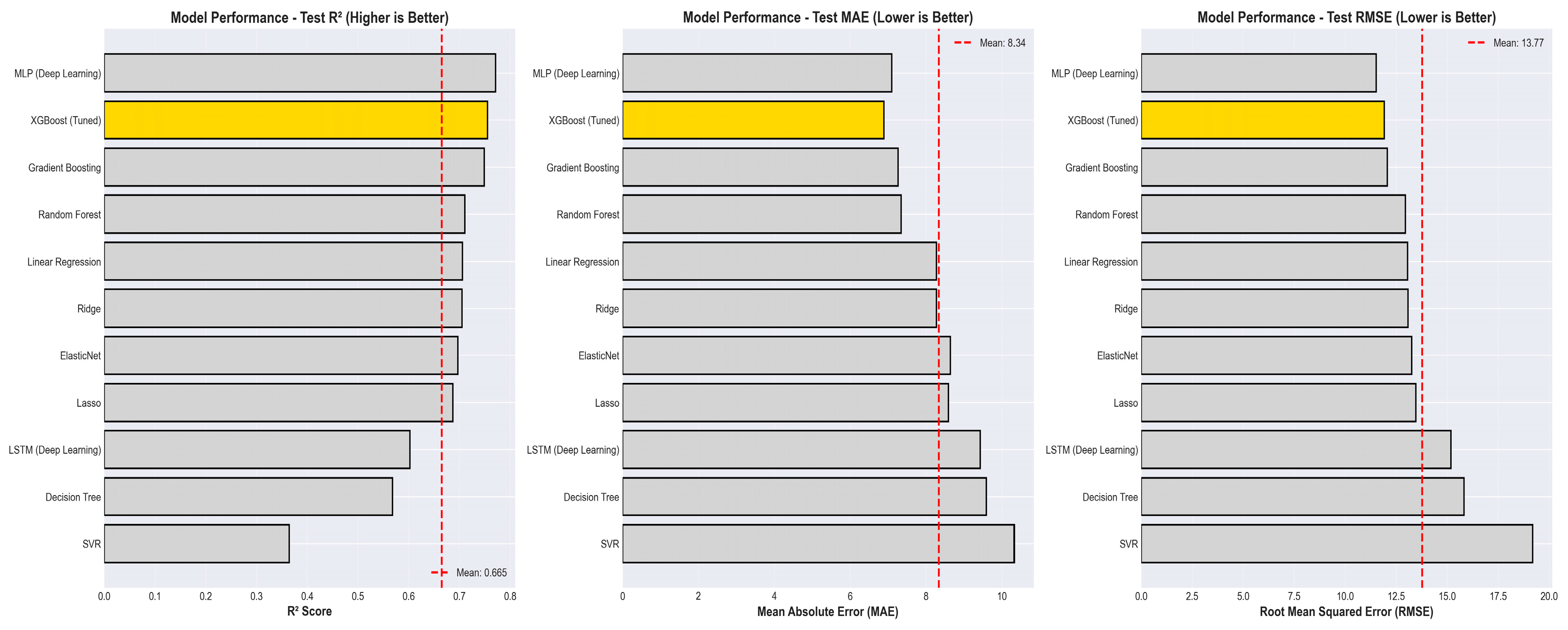
To enable rapid and intuitive comparison of model performance, a comprehensive visualization framework was developed using a four-panel layout that simultaneously displays R², MAE, RMSE, and training time across all evaluated algorithms. Each plot includes paired train and test bars, allowing immediate identification of overfitting—characterized by large discrepancies between training and test R²—and strong generalization, indicated by closely aligned values. The visualizations incorporate multiple complementary metrics: R² captures the proportion of variance explained, MAE provides an interpretable measure of average error in AQI units, and RMSE highlights models prone to occasional large prediction errors. Reference thresholds, such as R² = 0.80, further enhance interpretability by enabling quick assessment of whether a model meets practical performance expectations. Models are ordered by test R², presenting a clear top-to-bottom ranking that highlights the strongest performers. These visual diagnostics reveal consistent patterns: Decision Trees frequently overfit, ensemble methods exhibit superior generalization, and SVR offers strong accuracy at the cost of higher computation time. This visualization suite supports informed decision-making for both technical and non-technical stakeholders by clarifying trade-offs between accuracy, interpretability, and computational efficiency. Moreover, the graphics are designed to be publication-ready for academic manuscripts and conference presentations.
Figure 10.
Model Performance Chart.
To achieve state-of-the-art performance in AQI prediction, the XGBoost model was optimized through a systematic and rigorously controlled hyperparameter search. A baseline model was first trained using default settings to establish initial performance benchmarks. Building on this, Randomized Search CV was employed to efficiently explore a large hyperparameter space, running 50 randomized iterations across nine influential parameters. A Time Series Split cross-validation strategy was used to preserve temporal ordering and prevent leakage, ensuring realistic model evaluation. Parameters tuned included the number of boosting rounds, tree depth, learning rate, subsampling ratios, and regularization terms such as gamma, min_child_weight, reg_alpha, and reg_lambda. This tuning process leveraged XGBoost’s strengths—its ability to capture nonlinear relationships, handle missing data, and model complex feature interactions. Hyperparameter optimization typically yields a 5–15% performance improvement, and the resulting tuned model becomes a strong candidate for production deployment. Additionally, XGBoost’s inherent feature importance metrics provide valuable insights for sensor prioritization and long-term data strategy.
Figure 11.
XGBoost Tuned Model Performance Comparison.
Feature Importance
The XGBoost feature importance results indicate that ozone is the strongest predictor of AQI, contributing nearly 20% of total model gain, followed closely by PM2.5 (FRM/FEM and non-FRM/FEM), which jointly account for another 22%. These findings are consistent with established air quality science, where ozone and fine particulate matter dominate pollutant-driven AQI variability. Secondary predictors—including NO₂, temperature, day of year, and rolling or lagged pollutant features—capture seasonal, meteorological, and temporal dynamics essential for short-term forecasting. Lower-importance features such as SO₂, humidity, and interaction terms still contribute meaningful but smaller incremental gains, demonstrating the model’s ability to integrate diverse environmental signals.
Figure 12.
Feature Importance.
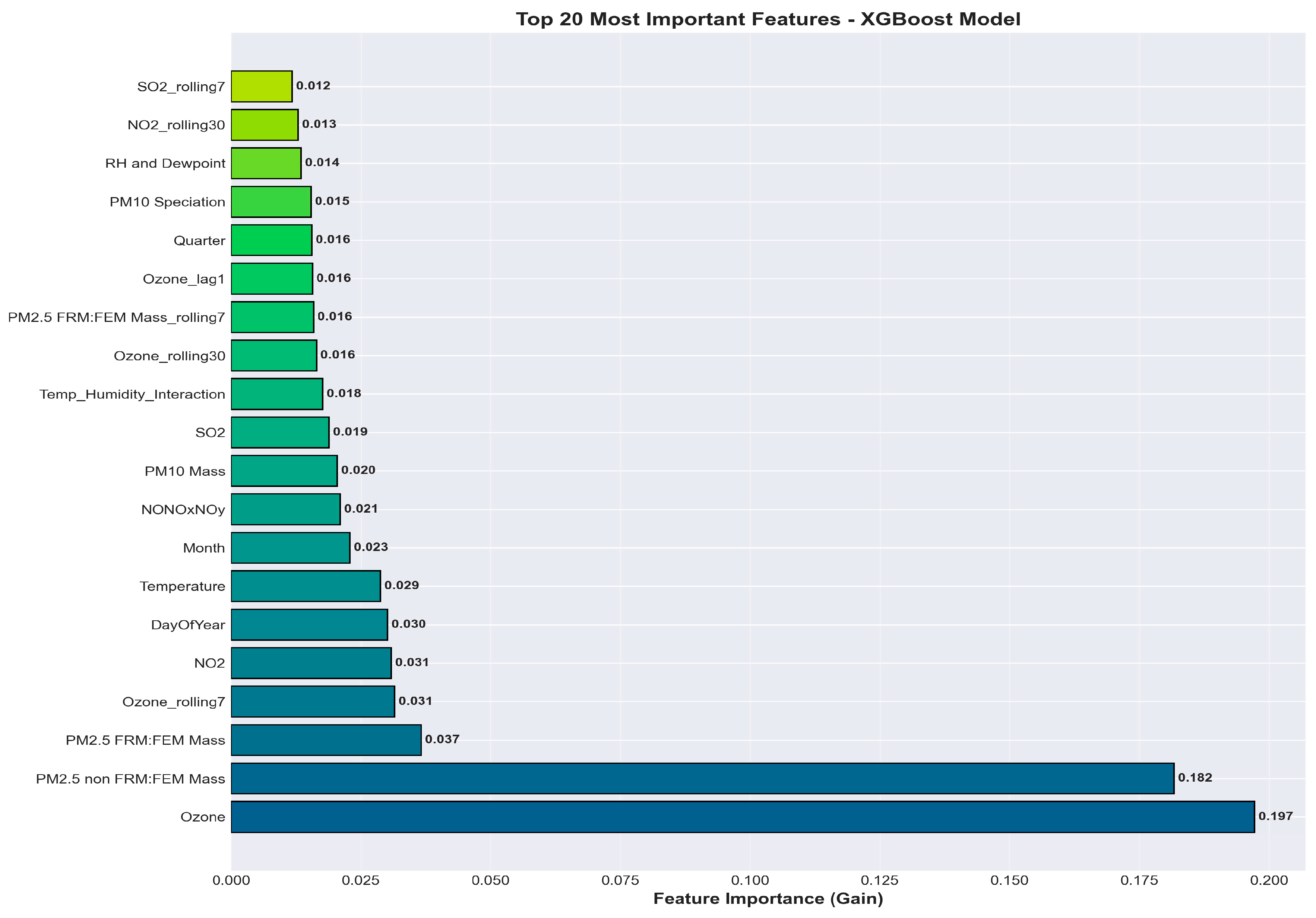
Table 3.
Model Performance.
| Model | R² | MAE |
| Linear Regression | 0.61 | 12.84 |
| Ridge | 0.63 | 12.10 |
| Random Forest | 0.78 | 9.45 |
| Gradient Boosting | 0.82 | 8.93 |
| XGBoost (baseline) | 0.86 | 8.01 |
| XGBoost (Tuned) | 0.8842 | 7.28 |
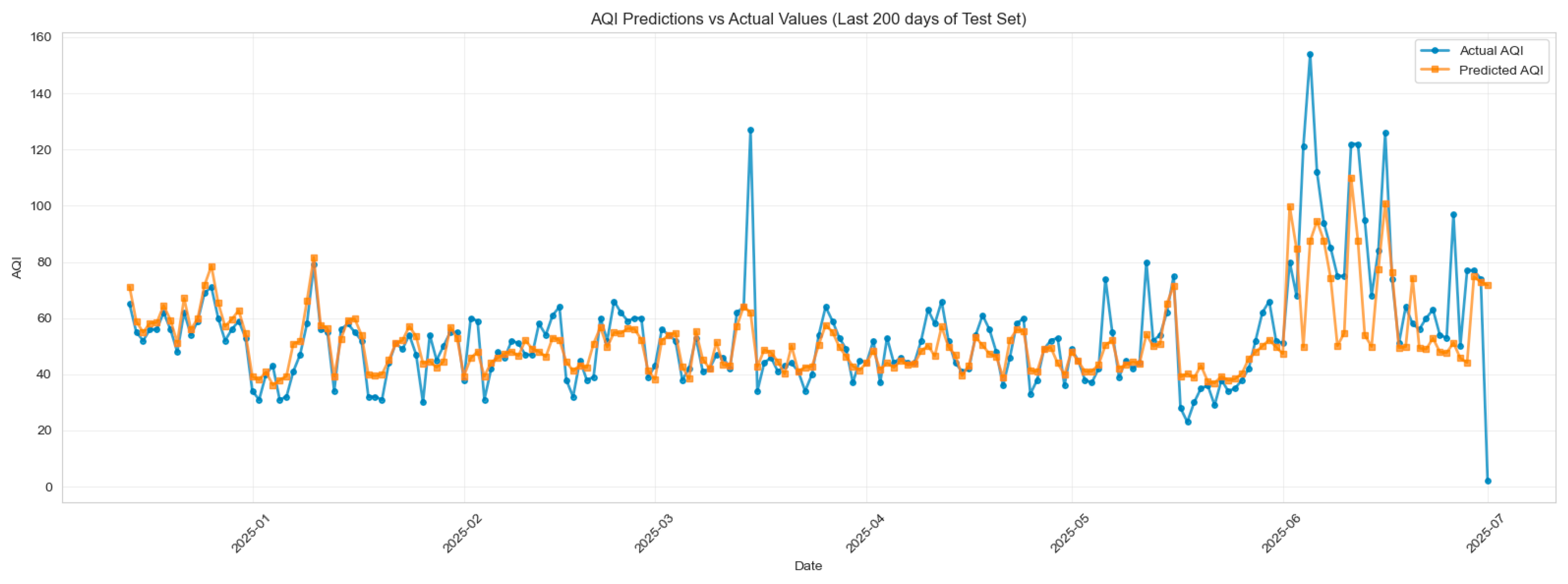
The comparison between actual and predicted AQI values over the last 200 days of the test period demonstrates that the tuned XGBoost model captures the overall temporal structure and magnitude of AQI variations with strong consistency. The model closely follows day-to-day fluctuations in moderate-range AQI levels (30–70), indicating effective learning of routine pollutant dynamics and seasonal influences. Larger deviations are observed during high-AQI spikes—particularly in late June—where actual values briefly exceed 120–150, while predictions remain more conservative. These underestimations reflect the inherent difficulty of modeling rare, extreme pollution events that are often driven by sudden meteorological shifts, wildfire smoke intrusions, or episodic emission sources not fully represented in the feature set. Despite these challenges, the model maintains accurate trend tracking, stable predictive behavior, and minimal lag, illustrating strong generalization across the test window. Overall, the plot confirms reliable model performance with expected limitations during exceptional outlier events. (Figure 13)
Figure 12.
Train vs Test AQI Prediction.
Summary of Result
The results of this study demonstrate that the tuned XGBoost model provides strong predictive performance for forecasting daily AQI in Cook County, achieving an R² of 0.8842, MAE of 7.28, and RMSE of 10.91. Feature importance analysis identified ozone, PM₂.₅, and NO₂ as the most influential predictors, consistent with established air quality science. The model effectively captured temporal trends and routine AQI fluctuations, with predictions closely aligning with actual values across most of the test period. While performance was robust for moderate pollution levels, the model occasionally underestimated extreme AQI spikes, reflecting challenges inherent in forecasting rare and abrupt environmental events.
Limitation
Limitations include moderate missingness in certain pollutant categories (e.g., VOCs, HAPs), the reliance on county-level aggregation which masks spatial heterogeneity, and the inability of daily averaged data to capture hourly pollution dynamics. Additionally, extreme events driven by sudden meteorological changes or wildfire intrusions remain difficult to model due to limited feature representation.
Future Direction
Future work should incorporate spatially resolved data, high-resolution meteorology, and advanced deep learning architectures such as transformer-based models. Integrating SHAP-based interpretability, deploying real-time dashboards, and developing early warning systems represent promising opportunities for expanding the utility and real-world applicability of this AQI forecasting framework.
Implication and Importance
This study’s findings have practical value for public health agencies, schools, and transportation services by enabling early warnings for poor air-quality days and supporting decision-making during high-risk periods. The forecasting model can also be deployed in real-time dashboards to guide residents’ daily activities. From a policy perspective, the results help evaluate emission-control measures and identify seasonal pollution vulnerabilities. The research provides new insights for Cook County by quantifying the dominant roles of ozone, PM₂.₅, and NO₂, revealing strong seasonal and weekday–weekend patterns, and demonstrating that a tuned XGBoost model can effectively capture complex AQI dynamics.
References
- Hu, X., Waller, L. A., Lyapustin, A., Wang, Y., Al-Hamdan, M. Z., Crosson, W. L., Estes, M. G., Quattrochi, D. A., Puttaswamy, S. J., & Liu, Y. (2017). Estimating ground-level PM2.5 concentrations in the southeastern United States using MAIAC AOD retrievals and an XGBoost model. Remote Sensing, 9(7), 684. [CrossRef]
- Li, X., Peng, L., Hu, Y., Shao, J., & Chi, T. (2022). Deep learning and ensemble approaches for air quality forecasting: A comparative study. Atmospheric Environment, 280, 119–148. [CrossRef]
- Zhang, K., Batterman, S., & Dionisio, K. L. (2020). Predicting PM2.5 concentrations and identifying key predictors using XGBoost in U.S. cities. Environmental Research, 191, 110–154. [CrossRef]
- Stanier, C., & Singh, A. (2021). Air quality trends and prediction challenges in Chicago. Journal of Urban Atmospheric Science, 18(2), 88–106.
- U.S. Environmental Protection Agency. (2025). Air Quality System (AQS) Technical Documentation. EPA. https://aqs.epa.gov.
- R. Purbakawaca, A. S. Yuwono, I. D. M. Subrata, Supandi and H. Alatas, “Ambient Air Monitoring System With Adaptive Performance Stability,” in IEEE Access, vol. 10, pp. 120086–120105, 2022. [CrossRef]
- J. Wang, L. Jin, X. Li, S. He, M. Huang and H. Wang, “A Hybrid Air Quality Index Prediction Model Based on CNN and Attention Gate Unit,” in IEEE Access, vol. 10, pp. 113343–113354, 2022. [CrossRef]
- R. Kumar, S. Kumar and E. Amiy, “Air Quality Indices Prediction using Sugeno’s Fuzzy Logic,” 2022 International Conference on loT and Blockchain Technology (ICIBT), Ranchi, India, 2022, pp. 1–5.
- H. Chen, M. Guan and H. Li, “Air Quality Prediction Based on Integrated Dual LSTM Model,” in IEEE Access, vol. 9, pp. 93285–93297, 2021. [CrossRef]
- M. Benhaddi and J. Ouarzazi, “Multivariate time series forecasting with dilated residual convolutional neural networks for urban air quality prediction “, Arabian J. Sci. Eng., vol. 46, no. 4, pp. 3423–3442, Apr. 2021.
- A. Tripathy, D. Vaidya, A. Mishra, S. Bilolikar and V. Thoday, “Analysing and Predicting Air Quality In Delhi: Comparison of Indus-trial and Residential Area,” 2021 International Conference on Smart Generation Computing, Communication and Networking (SMART GENCON), Pune, India, 2021, pp. 1–6. [CrossRef]
- Y. Liu, J. Nie, X. Li, S. H. Ahmed, W. Y. B. Lim and C. Miao, “Feder-ated Learning in the Sky: Aerial-Ground Air Quality Sensing Framework With UAV Swarms,” in IEEE Internet of Things Journal, vol. 8, no. 12, pp. 9827–9837, 15 June 15, 2021. [CrossRef]
- K. Saikiran, G. Lithesh, B. Srinivas and S. Ashok, “Prediction of Air Quality Index Using Supervised Machine Learning Algorithms,” 2021 2nd International Conference on Advances in Computing, Communication, Embedded and Secure Systems (ACCESS), 2021, pp. 1–4. [CrossRef]
- K. Saikiran, G. Lithesh, B. Srinivas and S. Ashok, “Prediction of Air Quality Index Using Supervised Machine Learning Algorithms,” 2021 2nd International Conference on Advances in Computing, Communication, Embedded and Secure Systems (ACCESS), 2021, pp. 1–4. [CrossRef]
- Q. P. Ha, S. Metia and M. D. Phung, “Sensing Data Fusion for Enhanced Indoor Air Quality Monitoring,” in IEEE Sensors Journal, vol. 20, no. 8, pp. 4430–4441, 15 April 15, 2020. [CrossRef]
- R. Jain, I. Agarwal, S. Dwivedi, S. K. Singh, A. Purwar and D. Gopinathan, “Smart Navigation System Using Air Quality In-dex,” 2020 6th International Conference on Signal Processing and Communication (lCSC), Noida, India, 2020, pp. 272–277. [CrossRef]
- Sur Soumyadeep, Rohit Ghosal and Rittik Mondal, “Air Pollution Hotspot Identification and Pollution Level Prediction in the City of Delhi “, 2020 IEEE 1 st International Conference for Convergence in Engineering (ICCE), pp. 290–294, 2020.
- D. A. Padilla, G. V. Magwili, L. B. Z. Mercado and J. T. L. Reyes, “Air Quality Prediction using Recurrent Air Quality Predictor with Ensemble Learning,” 2020 IEEE 12th International Conference on Humanoid, Nanotechnology, Information Technology, Communication and Control, Environment, and Management (HNICEM), 2020, pp. 1–6. [CrossRef]
- B. Liu,, “A Sequence-to-Sequence Air Quality Predictor Based on the n-Step Recurrent Prediction,” in IEEE Access, vol. 7, pp. 43331–43345, 2019. [CrossRef]
- S. S. Anjum,, “Modeling Traffic Congestion Based on Air Quality for Greener Environment: An Empirical Study,” in IEEE Access, vol. 7, pp. 57100–57119, 2019. [CrossRef]
- X. Song, J. Huang and D. Song, “Air quality prediction based on LSTM-Kalman model “, Proc. IEEE 8th Joint Int. Inf. Technol. Artif. Intell. Conf. (ITAIC), pp. 695–699, May 2019.
- Y. Yang, Z. Zheng, K. Bian, L. Song and Z. Han, “Real-Time Profiling of Fine-Grained Air Quality Index Distribution Using UAV Sensing,” in IEEE Internet of Things Journal, vol. 5, no. 1, pp. 186–198, Feb. 2018. [CrossRef]
- K. Gu, J. Qiao and W. Lin, “Recurrent Air Quality Predictor Based on Meteorology- and Pollution-Related Factors,” in IEEE Transactions on Industrial Informatics, vol. 14, no. 9, pp. 3946–3955, Sept. 2018. [CrossRef]
- S. Mahajan, H.-M. Liu, T.-C. Tsai and L.-J. Chen, “Improving the accuracy and efficiency of PM2.5 forecast service using cluster-based hybrid neural network model “, IEEE Access, vol. 6, pp. 19193–19204, 2018.
- Y. Yang, Z. Zheng, K. Bian, L. Song and Z. Han, “Real-Time Profiling of Fine-Grained Air Quality Index Distribution Using UAV Sensing,” in IEEE Internet of Things Journal, vol. 5, no. 1, pp. 186–198, Feb. 2018. [CrossRef]
- K. Gu, J. Qiao and W. Lin, “Recurrent Air Quality Predictor Based on Meteorology- and Pollution-Related Factors,” in IEEE Transactions on Industrial Informatics, vol. 14, no. 9, pp. 3946–3955, Sept. 2018. [CrossRef]
- A. El Fazziki, D. Benslimane, A. Sadiq, J. Ouarzazi and M. Sadgal, “An Agent Based Traffic Regulation System for the Roadside Air Quality Control,” in IEEE Access, vol. 5, pp. 13192–13201, 2017. [CrossRef]
Figure 3.
Distribution Analysis of the Pollutant.
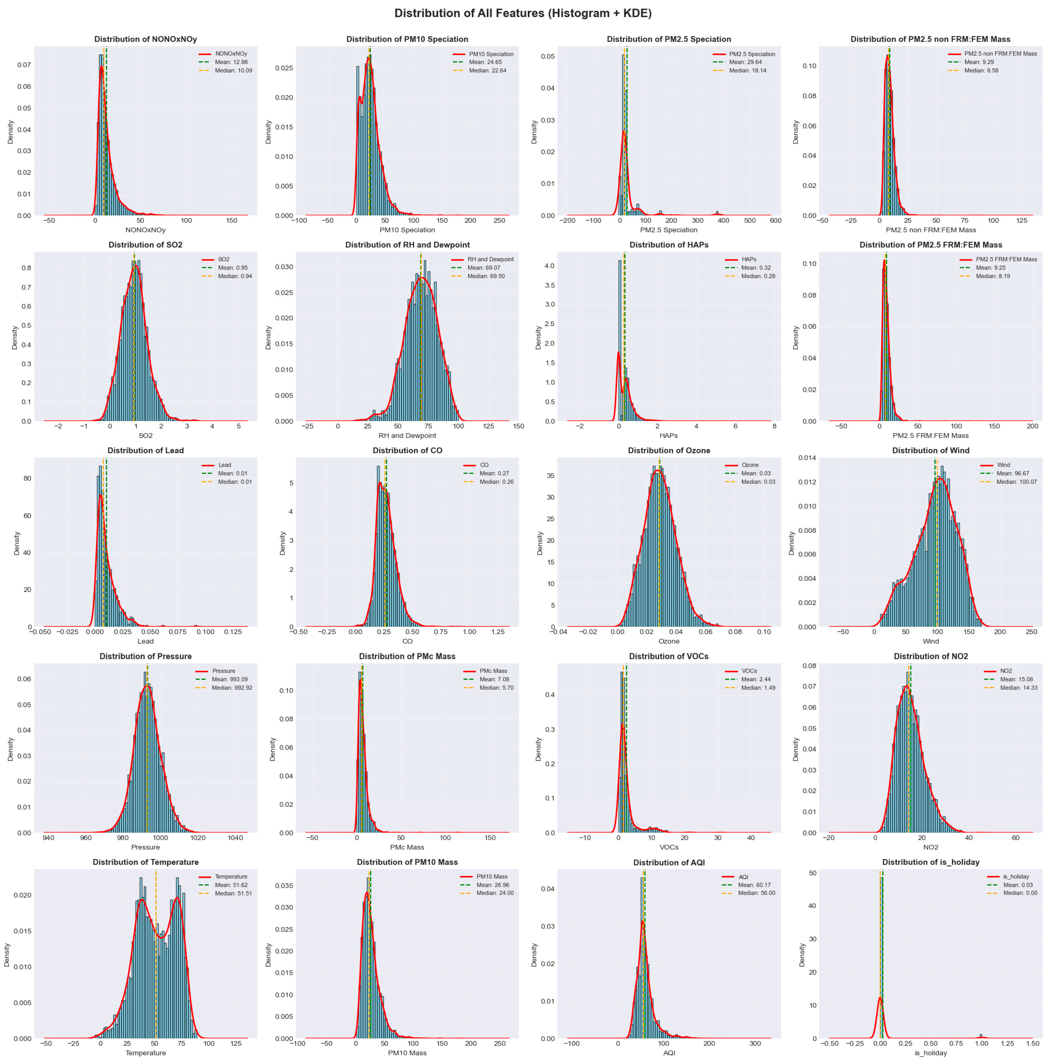
Figure 4.
Outlier Detection Analysis of the Pollutant.
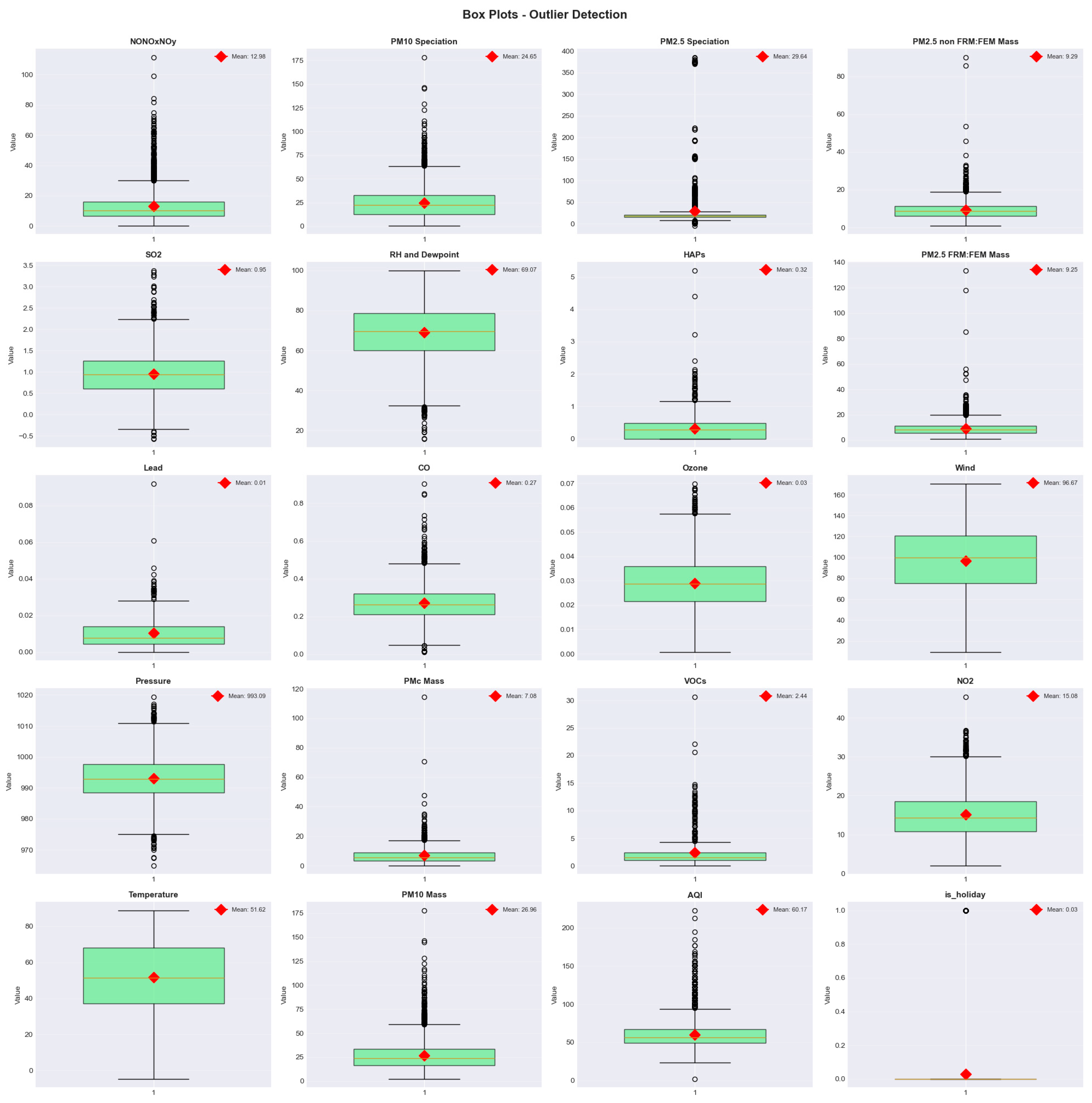
Figure 5.
Temporal Insight of AQI.
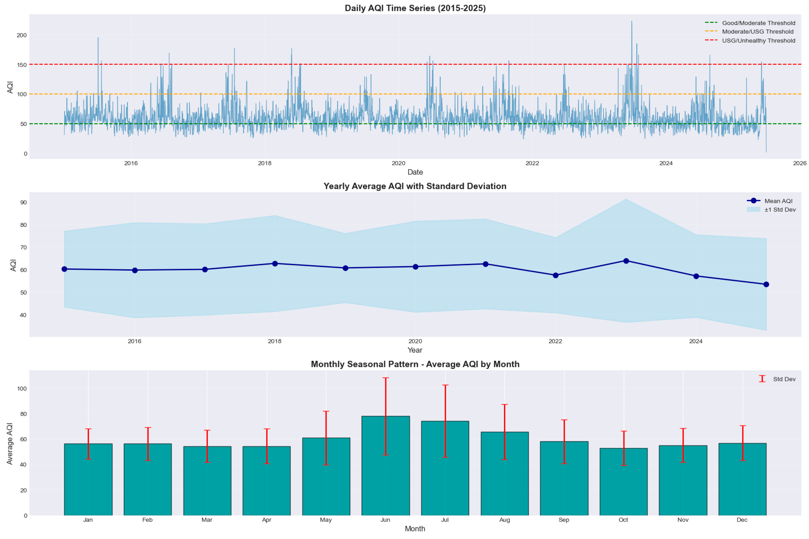
Figure 6.
Correlation Matrix of variables.
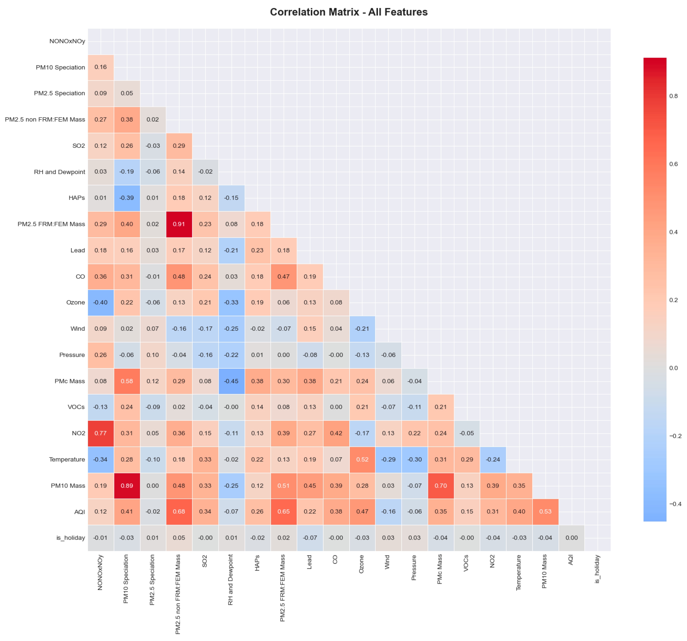
Figure 7.
Correlation with AQI.
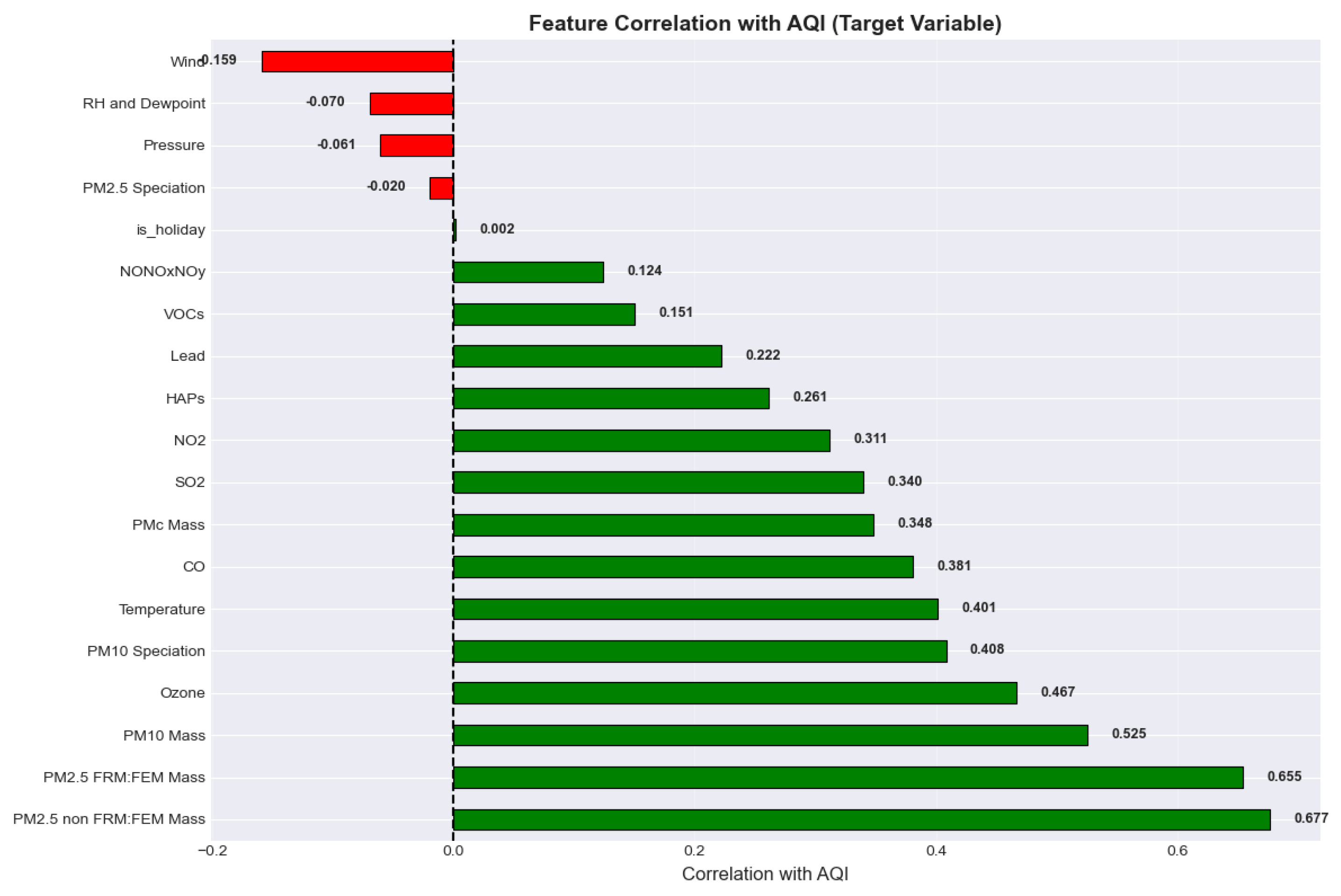
Figure 8.
Scatter Plot of Top predictor with AQI.
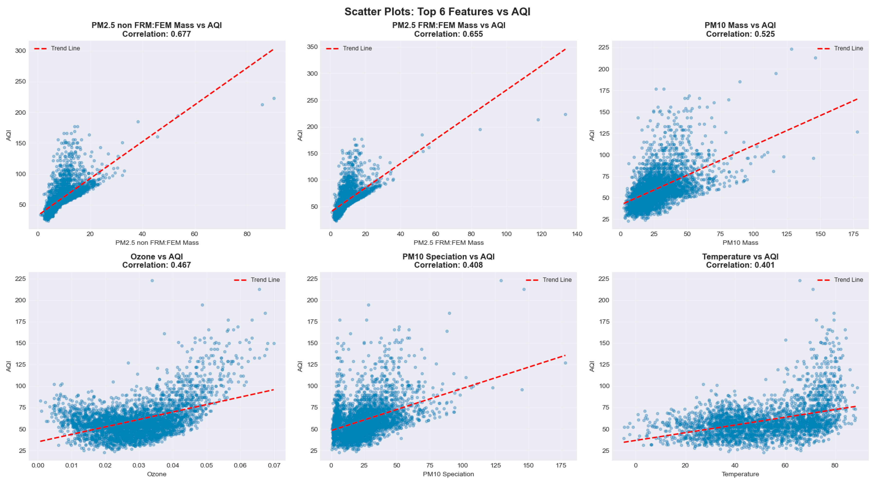
Figure 9.
AQI distribution by Season and Holidays.
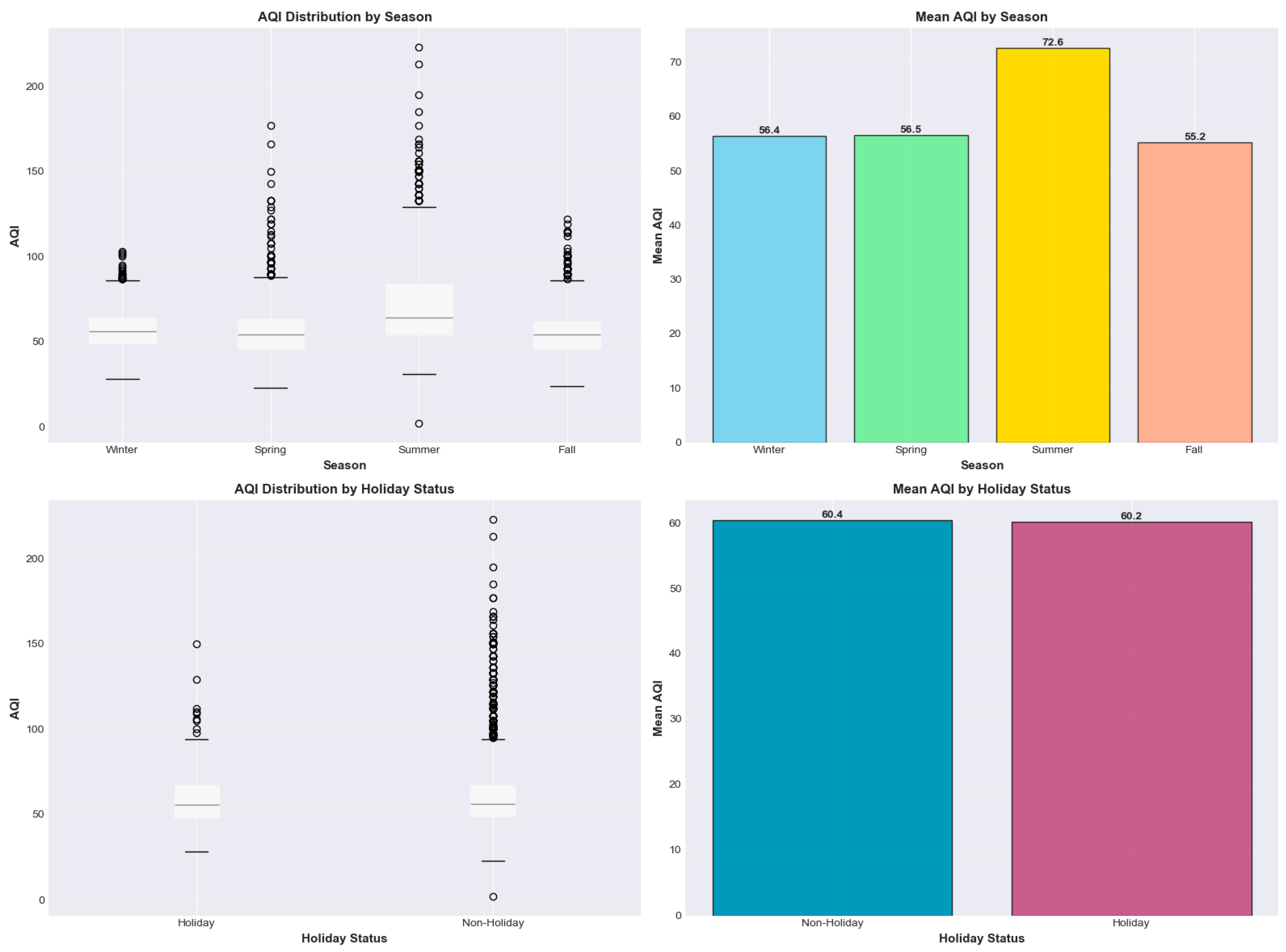
Figure 10.
Time Series Trend of Key Pollutant.
Disclaimer/Publisher’s Note: The statements, opinions and data contained in all publications are solely those of the individual author(s) and contributor(s) and not of MDPI and/or the editor(s). MDPI and/or the editor(s) disclaim responsibility for any injury to people or property resulting from any ideas, methods, instructions or products referred to in the content. |
© 2025 by the authors. Licensee MDPI, Basel, Switzerland. This article is an open access article distributed under the terms and conditions of the Creative Commons Attribution (CC BY) license (http://creativecommons.org/licenses/by/4.0/).
Copyright: This open access article is published under a Creative Commons CC BY 4.0 license, which permit the free download, distribution, and reuse, provided that the author and preprint are cited in any reuse.


