Submitted:
26 November 2025
Posted:
27 November 2025
You are already at the latest version
Abstract
This study conducts systematic experimental and numerical investigations to address the parameter calibration issue in the discrete element model of seashells, aiming to establish a high-fidelity numerical model that accurately characterizes their macroscopic mechanical behavior, thereby providing a basis for optimizing parameters of seashell crushing equipment. Firstly, intrinsic parameters of seashells were determined through physical experiments: density of 2.2 kg/m³, Poisson's ratio of 0.26, shear modulus of 1.57×10⁸ Pa, and elastic modulus of 6.5×10¹⁰ Pa. Subsequently, contact parameters between seashells and between seashells and 304 stainless steel, including static friction coefficient, rolling friction coefficient, and coefficient of restitution, were obtained via the inclined plane method and impact tests. The reliability of these contact parameters was validated by the angle of repose test, with a relative error of 5.1% between simulation and measured results. Based on this, using ultimate load as the response indicator, the Plackett-Burman experimental design was employed to identify normal stiffness per unit area and tangential stiffness per unit area as the primary influencing parameters. The Bonding model parameters were then precisely calibrated through the steepest ascent test and Box-Behnken design, resulting in an optimal parameter set. The error between simulation results and physical experiments was only 3.8%, demonstrating the high reliability and accuracy of the established model and parameter calibration methodology.
Keywords:
seashells
; discrete element method
; parameter calibration
; mechanical testing
1. Introduction
The global shellfish aquaculture industry has developed rapidly in recent years and has become an important part of the aquaculture industry. According to statistics from the Food and Agriculture Organization of the United Nations (FAO), China, as the world's largest shellfish aquaculture country, accounts for more than 80% of the global total output. In 2020, the output exceeded 16 million tons, with main species including oysters, clams, scallops, etc. [1]. Among them, freshwater mussels have become an important economic shellfish species in the waters of Lianyungang in recent years [2]. Freshwater mussels can be densely farmed, with a yield of 3-4 tons per 667 square meters. After removing the mussel columns and edges, a large amount of discarded mussel shells will be produced, accounting for about 80% of the total output. The discarded mussel shells are stinky and pungent, seriously affecting the environment [3]. At the same time, mussel shells are thin and light, making them very suitable as a substrate for the cultivation of nori filaments. The traditional method of cultivating nori filaments on mussel shells requires manual selection of shells, laying them flat at the bottom of the culture pond, and regular cleaning and water replacement. The cultivation period lasts for half a year, consuming a lot of human and material resources [4]. To improve the efficiency of nori aquaculture and solve the problem of mussel shell waste disposal, a cultivation plan will be studied that involves crushing mussel shells and pressing them into uniform-sized substrate blocks, combined with mechanical cleaning and water replacement equipment [5]. The crushed shells can also be used in multiple fields such as feed additives, building coatings, and cosmetics [6].
Due to the high hardness and brittleness of shells, traditional crushing methods are difficult to efficiently and uniformly crush shell materials into fine particles [7,8]. To improve the problems of low crushing efficiency, uneven product particle size, and dust pollution, it is necessary to explore the crushing mechanism of shells and optimize the structure of crushing equipment. The calibration of discrete element parameters for shells is the preliminary basis for the study of crushing equipment [9]. Therefore, the research on the calibration of discrete element parameters for the crushing of freshwater mussel shells is of great significance.
In recent years, the application of computer simulation and optimization design in agricultural engineering has become increasingly widespread. Among them, the discrete element method (DEM) has received significant attention due to its excellent modeling capabilities for materials and dynamic processes [10]. In discrete element modeling, various particle contact models have been proposed and applied to materials of different properties, such as the Hertz-Mindlin (HM) model, the Hertz-Mindlin with Bonding (HMB) model, the Johnson-Kendall-Robert (JKR) model, and various viscoelastic-plastic models (EEPA) [11]. The HM model, as the basic model, is often used to simulate the mechanical behavior of agricultural products such as grains and seeds, but it has shortcomings when dealing with particle systems with bonding structures and prone to fragmentation [12]. Therefore, the HMB model has been developed to describe the bonding and fracture processes between particles and has been successfully applied to the parameter calibration and fragmentation simulation of biological materials such as corn husk [13], tea stem [14], bone [15], lotus root [16], and beef [17]. The JKR model is used because it can effectively represent the surface adhesion effect and is applied to the simulation of high-humidity materials such as cow dung [18], fertilizer [19], pharmaceutical particles [20], and flour [21]. For materials with obvious viscoelastic-plastic characteristics such as fungal residue [22] and peat [23], the EEPA and other viscoelastic-plastic models show good applicability. Although there have been many achievements in the parameter calibration of discrete element parameters for agricultural materials, relevant research on shell materials is still relatively lacking. As a brittle and tightly bonded material, the physical properties of shells differ significantly from common agricultural materials, so a specialized modeling method needs to be developed. Based on the analysis of existing literature, the HMB model can effectively describe the mechanical response and failure process of such brittle bonded materials. Previous studies have used the HMB model to conduct discrete element modeling of bones and completed parameter calibration through the failure process of bonding keys, and this modeling and calibration method can provide a reference for the simulation of shell bending failure. Based on this, this paper selects the HMB model to establish a discrete element model of shells to make up for the lack of research in this field.
This paper takes the freshwater mussel as the research object and conducts the simulation modeling and parameter calibration work based on the discrete element method. Firstly, through the drainage method, uniaxial compression test, inclined plane method and collision test, the intrinsic parameters and contact parameters of the freshwater mussel were obtained [24,25,26,27]; subsequently, the Bonding model of the mussel shell was established by using the EDEM simulation software, and combined with the actual bending failure test, the PB test, the steepest slope climbing test and the response surface method, the key parameters such as the unit normal and tangential stiffness, critical normal and tangential stress, and bonding radius were calibrated [28,29,30,31]. By comparing the ultimate load obtained from the simulation and the physical test, the relative error was calculated to verify the accuracy of the calibrated Bonding parameters [32,33]. The establishment of this discrete element model of the freshwater mussel can provide a theoretical basis for the study of the shell fragmentation mechanism and the optimization of related crushing equipment [34].
2. Materials and Methods
2.1. Intrinsic Parameters of Shells
The materials used in this experiment were the shells of 3-year-old adult freshwater mussels from Lianyungang. The sampling method was random sampling. As shown in Figure 1, it was taken from the waters of Lianyungang. The test samples were measured using an electronic digital height gauge. The lengths of the mussel shells ranged from 132 to 149, the widths from 98 to 110, the heights from 19 to 22, and the thicknesses from 2.5 to 3.5. The volume of the mussel shells was measured using the drainage method, and their weights were measured using an electronic balance. The density of the mussel shells was calculated and found to be 2.2 kg/m³. The mussel shell waste was washed with clean water, the internal meat and external attachments were removed, the shells were polished with 2000-mesh sandpaper, and the fine impurities on the shells were removed by ultrasonic cleaning. They were then placed in a cool and ventilated place for natural drying. The inner shell was placed flat on the experimental table, and it was divided into three sections along the growth lines. The part near the starting point of growth was called the front part, the part near the edge was called the rear part, and the middle part was called the middle part. The line connecting the growth starting point to the farthest point on the shell edge was defined as the 0 growth line. Rotating α° forward along the 0 growth line obtained the α growth line. Mechanical cutting was performed in the area shown in Figure 2, and the middle area was selected for sample preparation. The sample was a 60mm-long, 6mm-wide, and 3mm-thick rectangular thin sheet [35].
The uniaxial compression test was conducted using an electronic high-temperature universal testing machine as shown in Figure 3. The experiment adopted the displacement control mode. The testing software MaterialTest 4.2 was turned on for online operation, and the test plan was set as the test method for organic irregular materials. The clam shell samples were placed on the tray in the order of the labels to ensure that no sliding along the tray would occur during the compression process, thereby avoiding measurement errors. A rigid flat punch was used. As the punch moved downward, a natural contact was formed between the punch and the clam shell, triggering the compression phenomenon. During the test, when the compressive force of the sample reached the preset limit value, the test could be stopped, and the testing machine would be disconnected.
This design is aimed at ensuring reliable data is obtained during the experiment and effectively controlling the progress of the experiment. Five repeated measurements were conducted on the size changes at the same marking position, and the average value was taken as the lateral compression deformation of the sample; at the same time, by measuring the height changes of the sample multiple times and taking the average value, the axial deformation of the sample was obtained. According to formulas (1-1), (1-2), and (1-3), the Poisson's ratio, shear modulus, and elastic modulus were determined to be 0.26, 1.57×10^8 Pa, and 6.5×10^10 Pa [36,37].
Elastic modulus formula:
In the formula, E represents the elastic modulus; F is the pressure; N; is the compression amount, in mm; the value of F/ is the slope of the straight line in the initial section of the compression curve; L is the height of the sample, in mm; A is the contact area between the sample and the indenter, in mm².
Shear modulus formula:
In the formula, G represents the shear modulus; E represents the elastic modulus (Young's modulus); ν represents the Poisson's ratio.
Poisson's ratio formula:
In the formula, ξt represents the transverse strain; ξa represents the axial strain.
2.2. Contact Parameters
2.2.1. Coefficient of Static Friction
The sample shells were placed separately on the shell powder bonding plate and the 304 stainless steel plate. The measured surface was fixed on a flat plate that could precisely adjust the inclination angle. Slowly lift one end of the plate, gradually increasing the angle θ between the plate and the horizontal plane. At this time, the gravitational force (mg) acting on the shell can be decomposed into two components: the component along the inclined plane (F), which is the driving force that causes object A to have a tendency to slide down. The component perpendicular to the inclined plane, which is equal to the normal force N, as per formula (2-1). As the angle θ increases, the sliding driving force F increases, and the maximum static friction force, as per formula (2-2), also changes accordingly. Critical state: When the angle θ increases to a certain value θₛ, the sliding driving force just exceeds the maximum static friction force, and object A begins to slide. By simplifying the above equation (with the mass m and gravitational acceleration g being cancelled out), the calculation formula for the static friction coefficient (2-3) can be obtained.
N = mg cosθ
μₛN = μₛ mg cosθ
μₛ=tanθₛ
Therefore, it is sufficient to precisely measure the critical angle θₛ at which the object begins to slide. The tangent value of this angle is the coefficient of static friction. Perform ten valid measurements in succession to obtain the range of the coefficient of static friction.
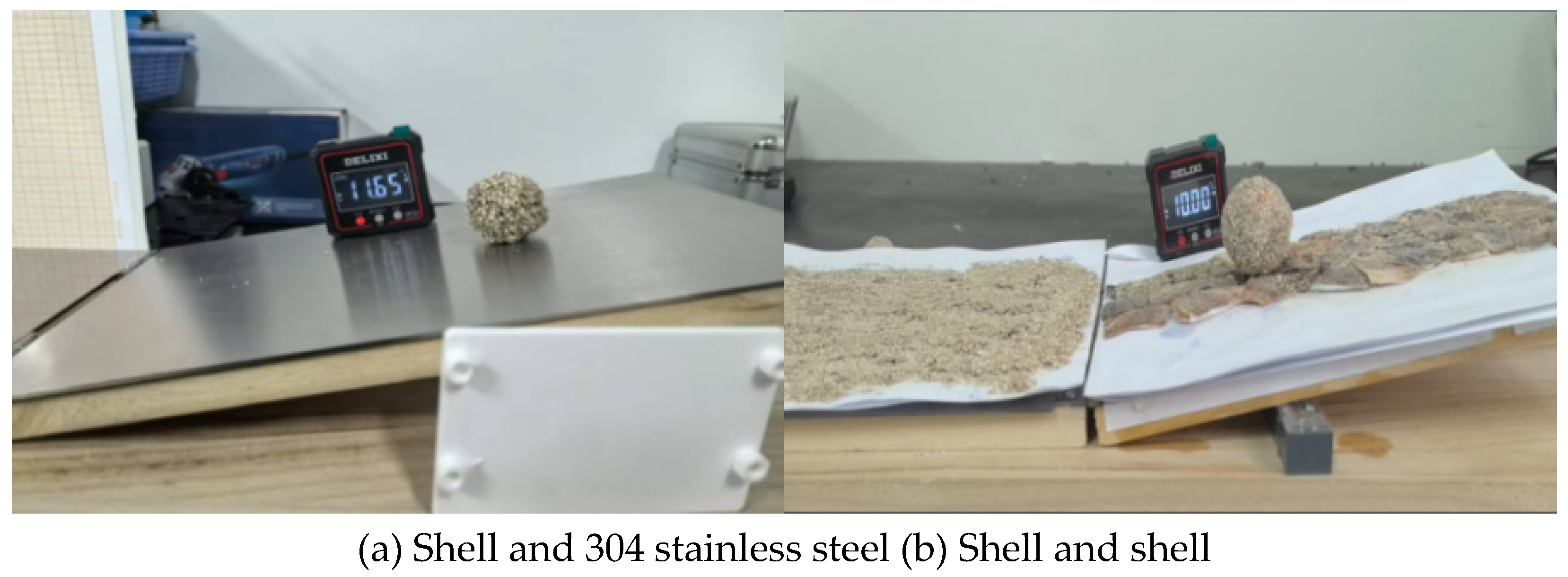
2.2.2. Rolling Friction Coefficient
After cleaning the shells, break them into pieces and grind them into uniform fine powder. Mix the shell powder with transparent epoxy resin in a certain proportion and pour it into a spherical mold to solidify and form. Place the solidified small balls on the shell powder bonding plate and the 304 stainless steel plate respectively. Slowly lift one end of the plate, increasing the inclination angle θ. When the small ball is in the critical rolling state, its force analysis is similar to static friction but the rolling friction coefficient is usually defined as the ratio of the resistance moment (M) to the normal force (N), that is, formula (2-4). Gravity generates a torque that causes it to roll downward, that is, formula (2-5), where R is the equivalent rolling radius of the small ball. The rolling friction resistance torque M hinders its rolling. Critical state: When the inclination angle reaches θᵣ, the sliding torque is exactly equal to the maximum rolling friction resistance torque. Formula (2-6), substitute the normal force N, and simplify to obtain the calculation formula for the rolling friction coefficient (2-7).
μᵣ = M / N
M= mg sinθ × R
mg sinθᵣ × R = M = μᵣ × N
N = mg cosθᵣ
mg sinθᵣ × R = μᵣ × mg cosθᵣ
μᵣ = R × tanθᵣ
Measure ten times in succession to obtain an effective measurement result, and then determine the range of the rolling friction coefficient.
Figure 4.
Static friction lift test.
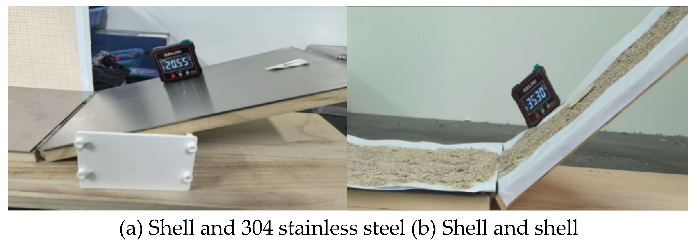
Figure 5.
Rolling friction lift test.
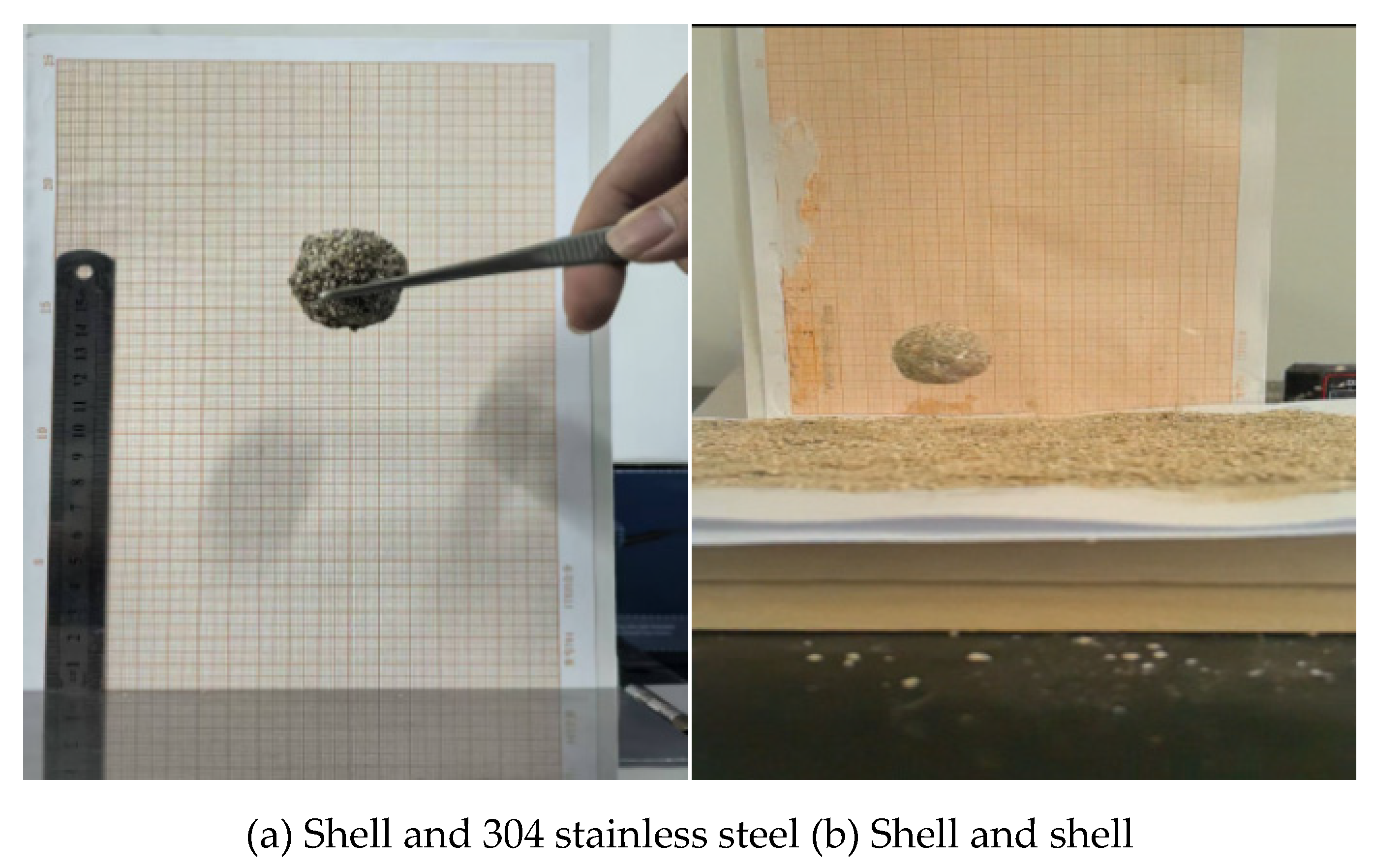
2.2.3. Collision Recovery Coefficient
The recovery coefficient is the ratio of the relative separation speed of the two objects after the collision to the relative approach speed before the collision. In the case of a small ball colliding with a huge, fixed plate, the change in the plate's velocity can be considered to be 0. Let the sample fall freely from a certain height H (with an initial velocity of 0). The speed u₁ of the sample before colliding with the target plate can be calculated using the law of conservation of energy, which is given by formula (2-8). After the collision, the sample bounces back with a speed v₁ and reaches a maximum rebound height h. According to the law of conservation of energy again, the rebound speed v₁ is as given by formula (2-9). Substitute u₁ and v₁ into the simplified recovery coefficient formula to obtain, formula (2-10).
u₁ = √(2gH)
v₁ = √(2gh)
e = √(h / H)
Therefore, only the drop height needs to be accurately measured.Therefore, only the drop height needs to be accurately measured. Release the shell sample at the predetermined height H, ensuring that the initial velocity is 0 and there is no initial rotation. Release the shell sample at the predetermined height H, ensuring that the initial velocity is 0 and there is no initial rotation. The base selects either the shell sheet or the 304 stainless steel sheet (with a mass much greater than the sample), and is rigidly fixed to ensure that the speed after the collision is almost 0. The base selects either the shell sheet or the 304 stainless steel sheet (with a mass much greater than the sample), and it is rigidly fixed to ensure that the velocity after the collision is almost 0. A high-precision and clear height scale is fixed beside the device. A high-precision and clear height scale is fixed beside the device. Use a high-speed camera to record the collision and rebound process, and through video frame analysis, accurately determine H and h. Retrieve the small ball and repeat this process 10 times to eliminate random errors. Use a high-speed camera to record the collision and rebound process, and through video frame analysis, accurately determine H and h. Retrieve the small ball and repeat this process 10 times to eliminate random errors.
Figure 6.
Shell ball drop test.
2.2.4. Angle of Restraint Test
Calculate the average value of the experimental data.Calculate the average value of the experimental data. The static friction coefficient, rolling friction coefficient, and collision recovery coefficient between shells and between shells and the surrounding environment are, respectively, 0.944, 0. The static friction coefficient, rolling friction coefficient, and collision recovery coefficient between shells and shells, as well as between shells and 304 stainless steel, are 0.129, and 0.944, 0.242.129, and 0.242 respectively. The static friction coefficient, rolling friction coefficient, and collision recovery coefficient between shells and 304 stainless steel are, respectively, 0.349, 0. The static friction coefficient, rolling friction coefficient, and collision recovery coefficient between shells and 304 stainless steel are 0.081, and 0.349, 0.367.081, and 0.367 respectively. The verification of the contact parameters of shells is carried out through the bucket rest angle test, as shown in Figure 7. The contact parameters of the shells were verified through the bucket rest angle test, as shown in Figure 7. Select 100mm inner diameter and 1mm diameter shell powder for physical experiments. Select shell powder with an inner diameter of 100mm and a diameter of 1mm for physical experiments. After repeating the tests 10 times, the average value is 27. After repeating the tests 10 times, the average value is 27.15°.15°. In the EDEM software, a simulation test with the s In the EDEM software, a simulation test with the same size is established.ame size was established. The intrinsic parameters and contact parameters were obtained from the previous experiments. The intrinsic parameters and contact parameters are obtained from the previous experiments. The simulation value is 25.76°, with a relative error of 5.The simulation value is 25.76°, with a relative error of 5.1%.1%. This indic This indicates that the data is reliable [27,38].ates that the data is reliable [27,38].
2.3. Three-Point Bending Failure Test and Bongding Model Parameters
2.3.1. Three-Point Bending Test
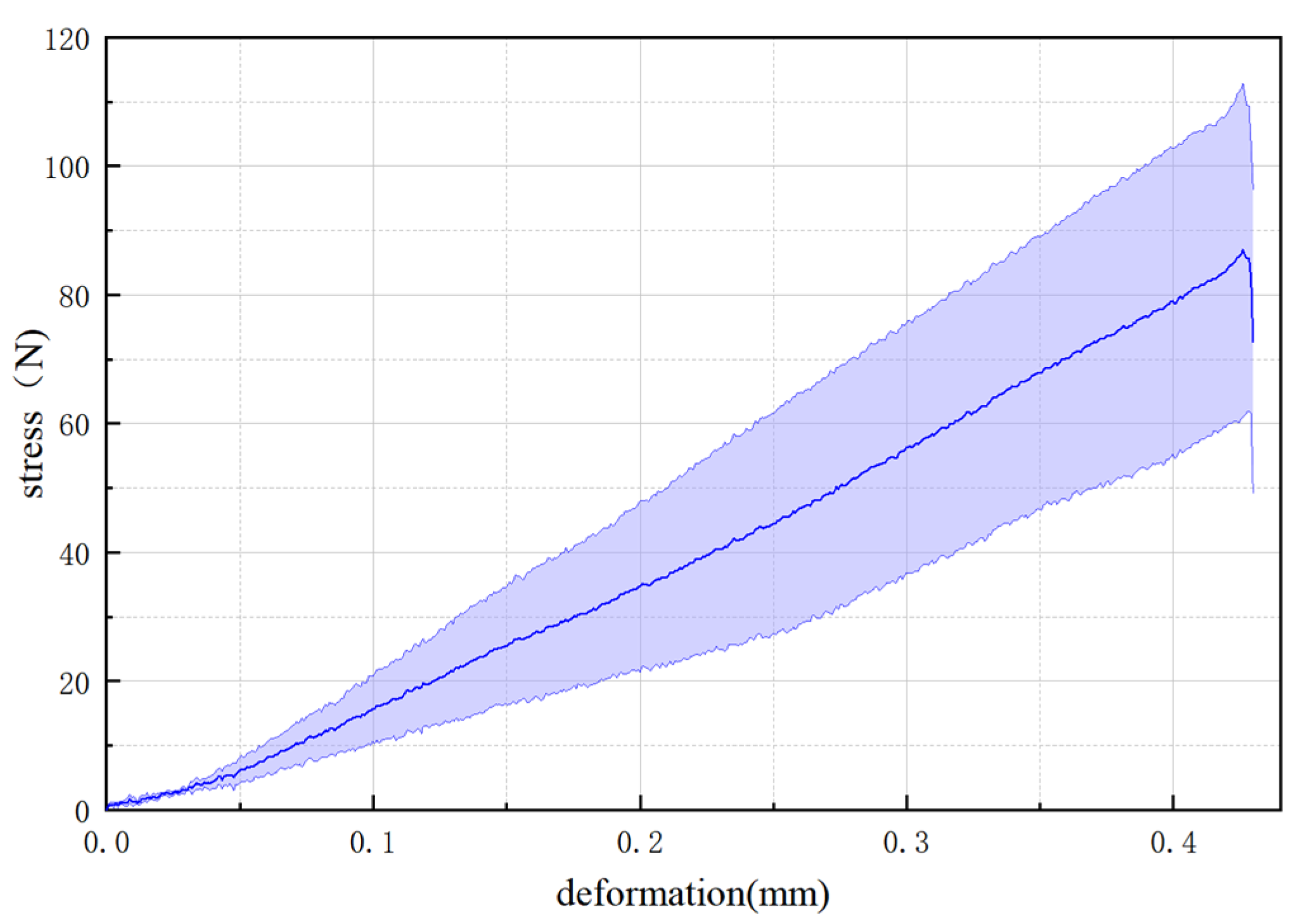
The maximum load measured through the three-point bending test was taken as the target value for the simulation of the Bonding parameters calibration test.The maximum load measured through the three-point bending test was taken as the target value for the simulation of the Bonding parameters calibration test. The curve dropped sharply at this point. The sample broke from the middle, splitting into two parts, and the crack was approximately a straight line. Thirty more tests were repeated and their average values were calculated [33], as shown in Figure 10.
Figure 8.
Three-point bending test.
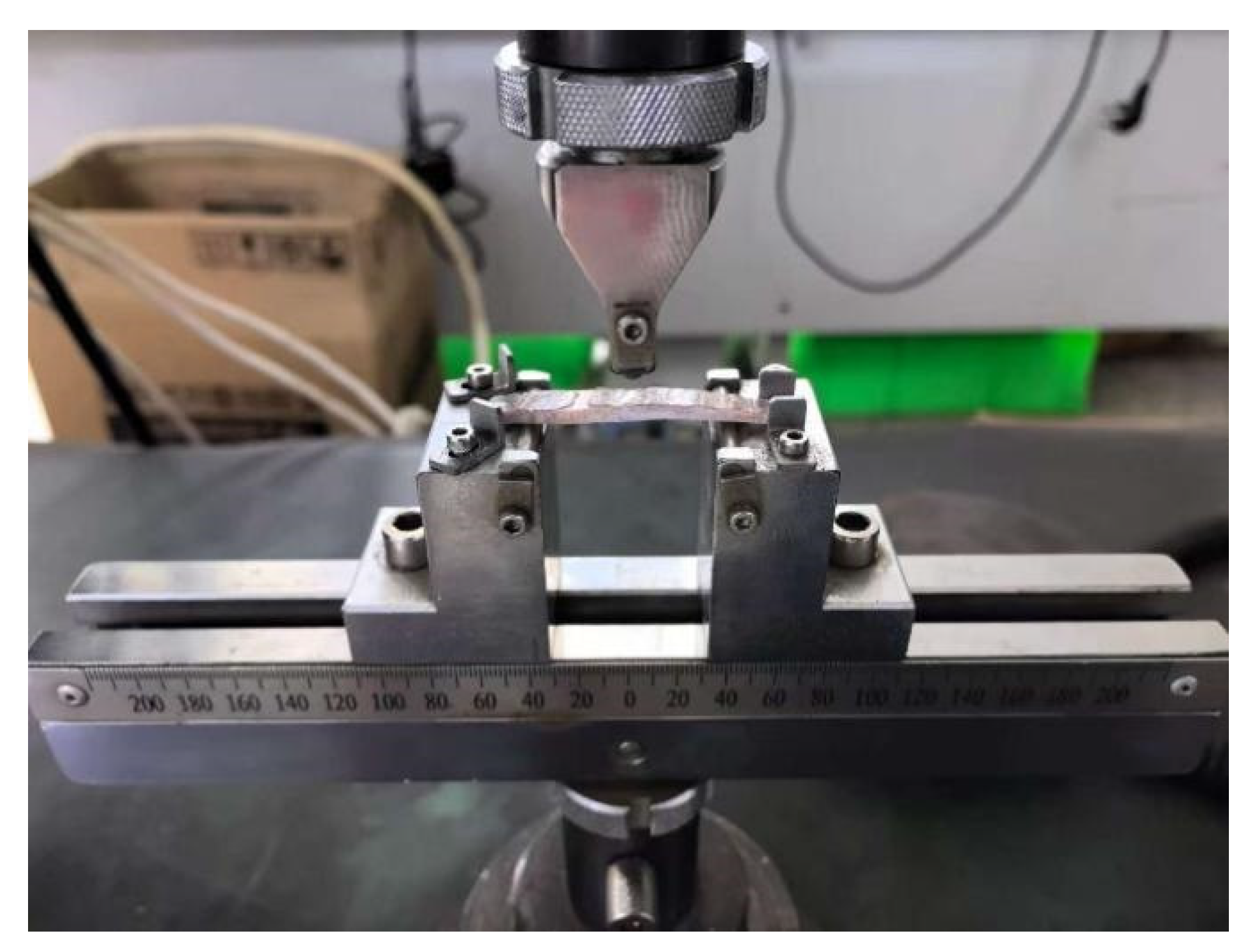
Figure 9.
The bending fracture condition of the sample.
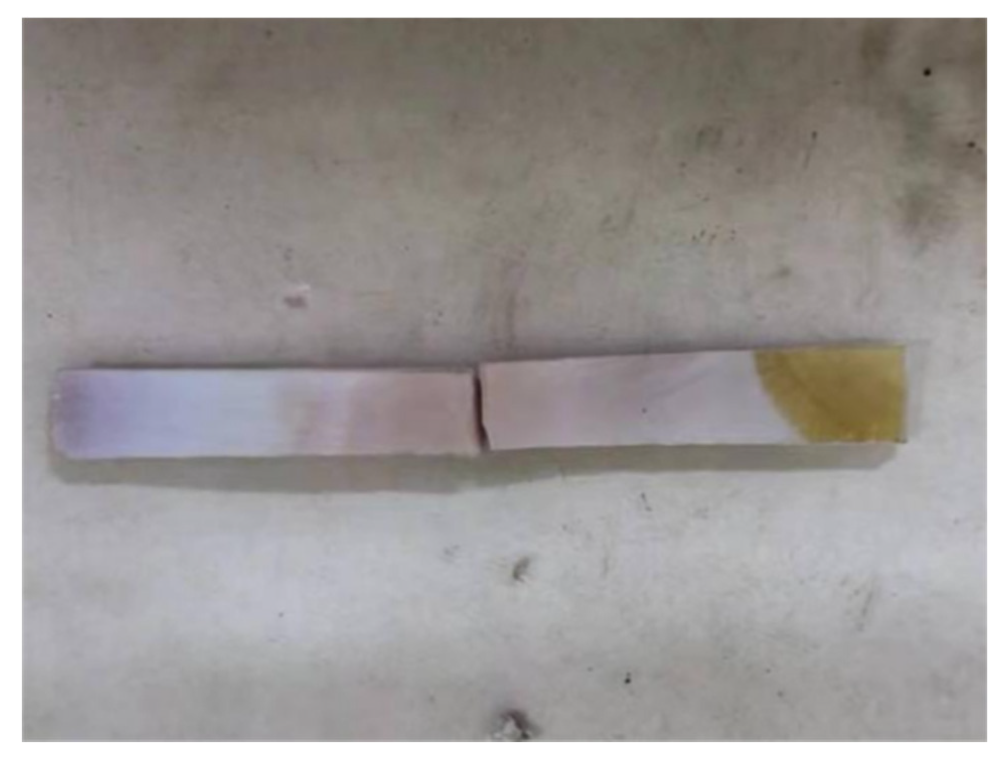
Figure 10.
Average load-displacement value.
2.3.2. Establishment of a Three-Point Bending Test Simulation Model
In the discrete element software EDEM, the BondingV2 model is adopted to simulate the mechanical response and failure process of shell-like biological materials under three-point bending load. The main parameters of the Bond key are normal stiffness, tangential stiffness, critical normal stress, critical tangential stress, and bonding radius, and these parameters need to be based on the intrinsic parameters and contact parameters measured in advance [39,40,41].
Based on the real structure of the shell sample, a geometric model of the same size and shape is simulated. Considering the time required for subsequent simulations, the particles are set as spherical particles with a diameter of 1mm, totaling 1080 particles. After exporting the coordinates of the generated particles, a flexible body is created, and the contact radius is set to 0.6mm, with a time step of 1.9195×10⁻⁶ to generate the Bond keys. A three-point bending simulation model consistent with the physical experiment size is established in EDEM, as shown in Figure 11. The upper punch and the two lower supports are set as rigid bodies. According to the average ultimate load in the actual experiment, the punch is set to -80N along the Z-axis. Based on the fracture situation of the shell experiment, the parameters of the Bond keys are continuously adjusted for reverse calibration.
Through a series of parameter pre-simulation experiments, the bonding stiffness and strength parameters are systematically adjusted to make the force-displacement curve, peak load, and failure mode obtained from the virtual simulation match the physical experiment results. The initial parameter range of the Bond keys is obtained, as shown in Table 1, and is used as the factor levels of the Plackett Burman test.
2.3.3. Plackett-Burman Experiment
To efficiently screen out the key factors that have significant statistical influence on the interface ultimate load from numerous potential influencing parameters, this study adopted the Plackett-Burman experimental design method [42]. The P-B design is an efficient two-level screening design that can evaluate the main effects of factors with the least number of experiments, making it highly suitable for identifying important factors in the initial stage. Five Bond parameters were selected as the factors to be studied in this research, namely: normal stiffness per unit area, shear stiffness per unit area, critical normal stress, critical shear stress, and bond radius. Each factor was set at high and low levels in the experiment, and the level values were determined based on previous theoretical research, material properties, and pre-experiment results. The experimental matrix was generated using the statistical software Design-Expert, and the experimental plan is presented in the table. The experimental results are shown in Table 2 and Table 3 and Figure 12. It can be seen that the normal stiffness and shear stiffness have extremely significant effects on the ultimate load, with P values all less than 0.0001, and the effect values on the target are positive. The normal stiffness, shear stiffness, and critical normal stress all have extremely significant effects on the ultimate displacement, with P values all less than 0.001, and the effect values on the target are positive.
** indicates extremely significant difference (P≤0.01), * indicates significant difference (0.01<P≤0.05), the same as below.
2.3.4. Hill-Climbing Test
With the ultimate load and ultimate displacement as the optimization targets, a climbing test was conducted for the unit normal stiffness, unit tangential stiffness, and critical normal stress, as shown in Table 4. During the test, based on the significant analysis results from the previous stage, other factors were fixed at specific levels, and the above three stiffness parameters were adjusted stepwise in a progressive manner. For each change in parameter level, a set of response data for the ultimate load and ultimate displacement was recorded, and the response trend was used to gradually approach the optimal region. This process, through systematic direction adjustment and stepwise search, effectively revealed the individual and coupled action mechanisms of the three stiffness parameters on the ultimate load and ultimate displacement, providing experimental basis and direction guidance for subsequent response surface optimization.
2.3.5. Response Surface Experiment
The objective of the experiment is to find a set of values for the unit area normal stiffness, unit area tangential stiffness, and critical normal stress that will make the simulation results of the shell sample's bending failure most consistent with the actual physical test results. Based on the results of the climbing test, the fourth to sixth groups were selected as the BBD test range. BBD is suitable for experimental designs with 2 to 5 dependent variables and can efficiently construct a second-order response surface model with a small number of experiments, making it very suitable for this scenario. The Box-Behnken response surface experiment was conducted using the Design-Expert software. For each parameter combination of the BBD design, a bending failure simulation was run and the response values of the ultimate load and ultimate displacement were recorded, as shown in Table 5. Based on the simulation results, a second-order mathematical model was established between the unit area normal stiffness, unit area tangential stiffness, critical normal stress and the response values, formula (3-1), and the optimal parameter combination was sought. The test plan and results, as well as the variance analysis results, are shown in Table.
Fmax=84.6+3.25X1+1.62X2+0.375X3+0.25X1X2-0.25X1X3-0.05X12+0.2X22+0.7X32
Smax=0.428+0.0162X1+0.0075X2+0.0062X3-0.0025X1X2-0.005X1X3-0.0025X2X3-0.0015X12+0.001X22-0.0015X32
From Table 6, it can be seen that the model determination coefficient R2 is 0.9444 and 0.9667, indicating good fit; the model is significant and the non-fit term is not significant, suggesting high model accuracy. X1 and X2 have extremely significant effects on the ultimate load (P < 0.01), and X1, X2, and X3 have extremely significant effects on the ultimate displacement (P < 0.01). The interaction and squared terms of X1, X2, and X3 have no significant effect on the ultimate load (P > 0.05), while the interaction term of X1 and X3 has a significant effect on the ultimate displacement (P < 0.05), and the interaction and squared terms of the other X1, X2, and X3 have no significant effect on the ultimate displacement (P > 0.05). The response surface diagrams of the ultimate load and ultimate displacement obtained from the regression equation are shown in Figure 13.
2.3.6. Verification Test
The optimization solution was obtained using the Design-Expert software, resulting in X1, X2, X3, X4, and X5 being 8.26×10^10, 1.116×10^10, 4.438×10^7, 4×10^7, and 0.5 respectively. The optimal parameters obtained were then substituted into the EDEM simulation model, and the bending test was re-run, as shown in Figure 14. The degree of consistency between the deformation-load curve of this simulation, the crack analysis, and the physical test was compared. The relative error compared to the actual test was 3.8%, which is basically consistent with the average value of the actual test, indicating that the modeling and calibration parameters of the shell sample are accurate and reliable [34].
3. Conclusions
This paper carried out the calibration of the parameters of the shell discrete element model, aiming to construct a high-fidelity numerical model that can accurately reproduce its macroscopic mechanical behavior. This is to provide a reference for the parameter optimization of the shell crushing equipment.
- (1)
- The intrinsic parameters of the shells were determined through the experimental method. The three-dimensional size range of the shells was measured. Due to the diverse shapes of the shells, shell samples of the same size had to be fabricated. The density was measured to be 2.2 kg/m³ using the drainage method. Through uniaxial compression tests and calculations, the Poisson's ratio, shear modulus, and elastic modulus of the shells were obtained, which were 0.26, 1.57×10^8 Pa, and 6.5×10^10 Pa, respectively.
- (2)
- The static friction coefficient, rolling friction coefficient, and collision recovery coefficient between shells and shells were measured by the inclined plane method and collision tests, which were 0.944, 0.129, and 0.242 respectively. The static friction coefficient, rolling friction coefficient, and collision recovery coefficient between shells and 304 stainless steel were 0.349, 0.081, and 0.367 respectively. The reliability of the data was verified by the angle of repose test. The shape of the shells has a significant influence on the accumulation angle in the actual test, and the test results cannot be accurately obtained. Therefore, shell powder was used. The relative error between the simulated values and the real values was 5.1%. This indicates that the data is reliable.
- (3)
- Using the actual ultimate load as the response value, the Bonding parameters were calibrated by the simulation approximation prediction method. Through the Plackett-Burman experimental design, the normal stiffness and tangential stiffness were selected as the significant parameters affecting the ultimate load. The range of significance parameters for calibration was narrowed by the steepest ascent test. On this basis, the Box-Behnken experimental design method and variance analysis were adopted to precisely calibrate the two significant parameters in the Bonding model. Finally, the optimal parameter combination was obtained: the unit area normal stiffness, the unit area tangential stiffness, the critical normal stress, the critical tangential stress, and the bonding radius, which were 8.26×10^10 N/m^3, 1.116×10^10 N/m^3, 4.438×10^7 Pa, 4×10^7 Pa, and 0.5 mm respectively. The error compared with the actual test was 3.8%, verifying the reliability of the shell modeling and the calibrated parameters.
Acknowledgments
This study was supported by the Youth Fund of Natural Science Foundation of Jiangsu Province (BK20241058) and the Project of Graduate Student Scientific Research and Practical Innovation Program of Jiangsu Ocean University (KYCX2024-41).
References
- QIAN J, FUJING DENG, SHUMWAY S E, 等. The thick-shell mussel Mytilus coruscus: Ecology, physiology, and aquaculture[J/OL]. Aquaculture, 2024, 580: 740350. [CrossRef]
- WANG F, WALL G. Mudflat development in Jiangsu Province, China: Practices and experiences[J/OL]. Ocean & Coastal Management, 2010, 53(11): 691-699. [CrossRef]
- CHUANG H C, WANG S Y, CHENG A C. Research on and application of low-temperature calcination on waste Taiwanese hard clam shell during Taiwanese hard clam aquaculture[J/OL]. Aquaculture, 2024, 590: 741048. [CrossRef]
- XIAOLEI F, GUANGCE W, DEMAO L, 等. Study on early-stage development of conchospore in Porphyra yezoensis Ueda[J/OL]. Aquaculture, 2008, 278(1-4): 143-149. [CrossRef]
- FAKAYODE O, A. Size-based physical properties of hard-shell clam (Mercenaria mercenaria) shell relevant to the design of mechanical processing equipment[J/OL]. Aquacultural Engineering, 2020, 89: 102056. [CrossRef]
- DERKACH S, KRAVETS P, KUCHINA Y, 等. Mineral-free biomaterials from mussel (Mytilus edulis L.) shells: Their isolation and physicochemical properties[J/OL]. Food Bioscience, 2023, 56: 103188. [CrossRef]
- IWASE K, HARUNARI Y, TERAMOTO M, 等. Crystal structure, microstructure, and mechanical properties of heat-treated oyster shells[J/OL]. Journal of the Mechanical Behavior of Biomedical Materials, 2023, 147: 106107. [CrossRef]
- LV J, JIANG Y, ZHANG D. Structural and Mechanical Characterization of Atrina Pectinata and Freshwater Mussel Shells[J/OL]. Journal of Bionic Engineering, 2015, 12(2): 276-284. [CrossRef]
- OSA J L, MONDRAGON G, ORTEGA N, 等. On the friability of mussel shells as abrasive[J/OL]. Journal of Cleaner Production, 2022, 375: 134020. [CrossRef]
- 基于科学计量的中国农业工程研究热点探析_师丽娟[Z].
- 离散元法在农业工程研究中的应用现状和展望_曾智伟[Z].
- MARAVEAS C, TSIGKAS N, BARTZANAS T. Agricultural processes simulation using discrete element method: a review[J/OL]. Computers and Electronics in Agriculture, 2025, 237: 110733. [CrossRef]
- HAN D, TANG C, LIU B, 等. Hierarchical model acquisition and parameter calibration of the corncob based on the discrete element method[J/OL]. Advanced Powder Technology, 2025, 36(7): 104932. [CrossRef]
- 茶茎秆离散元模型参数标定与试验_杜哲[Z].
- 冷鲜波尔山羊肋骨弯曲破坏离散元参数标定_卫佳[Z].
- 莲藕主藕体弯曲破坏离散元仿真分析_焦俊[Z].
- 基于离散元法的牛肉咀嚼破碎模型构建_王笑丹[Z].
- 玉米秸秆-牛粪混料离散元仿真参数标定与试验_马永财[Z].
- CHEN G, WANG Q, LI H, 等. Rapid acquisition method of discrete element parameters of granular manure and validation[J/OL]. Powder Technology, 2024, 431: 119071. [CrossRef]
- 健胃消食颗粒物性参数测定与离散元仿真参数标定_王子千[Z].
- 基于离散元法的面粉颗粒接触参数标定试验_陈硕[Z].
- 基于离散元法的香菇菌渣颗粒仿真物理参数标定_李震[Z].
- 基于单轴密闭压缩试验的草炭离散元参数标定_王斌斌[Z].
- SCHRAMM M, TEKESTE M Z, PLOUFFE C, 等. Estimating bond damping and bond Young’s modulus for a flexible wheat straw discrete element method model[J/OL]. Biosystems Engineering, 2019, 186: 349-355. [CrossRef]
- SADRMANESH V, CHEN Y. Simulation of tensile behavior of plant fibers using the Discrete Element Method (DEM)[J/OL]. Composites Part A: Applied Science and Manufacturing, 2018, 114: 196-203. [CrossRef]
- ZHANG S, ZHANG R, CAO Q, 等. A calibration method for contact parameters of agricultural particle mixtures inspired by the Brazil nut effect (BNE): The case of tiger nut tuber-stem-soil mixture[J/OL]. Computers and Electronics in Agriculture, 2023, 212: 108112. [CrossRef]
- DU C, HAN D, SONG Z, 等. Calibration of contact parameters for complex shaped fruits based on discrete element method: The case of pod pepper (Capsicum annuum)[J/OL]. Biosystems Engineering, 2023, 226: 43-54. [CrossRef]
- FANG M, YU Z, ZHANG W, 等. Friction coefficient calibration of corn stalk particle mixtures using Plackett-Burman design and response surface methodology[J/OL]. Powder Technology, 2022, 396: 731-742. [CrossRef]
- WANG S, YU Z, AORIGELE, 等. Study on the modeling method of sunflower seed particles based on the discrete element method[J/OL]. Computers and Electronics in Agriculture, 2022, 198: 107012. [CrossRef]
- SHI Y, JIANG Y, WANG X, 等. A mechanical model of single wheat straw with failure characteristics based on discrete element method[J/OL]. Biosystems Engineering, 2023, 230: 1-15. [CrossRef]
- ZHAO W, CHEN M, XIE J, 等. Discrete element modeling and physical experiment research on the biomechanical properties of cotton stalk[J/OL]. Computers and Electronics in Agriculture, 2023, 204: 107502. [CrossRef]
- SCHRAMM M, TEKESTE M Z. Wheat straw direct shear simulation using discrete element method of fibrous bonded model[J/OL]. Biosystems Engineering, 2022, 213: 1-12. [CrossRef]
- LEBLICQ T, SMEETS B, RAMON H, 等. A discrete element approach for modelling the compression of crop stems[J/OL]. Computers and Electronics in Agriculture, 2016, 123: 80-88. [CrossRef]
- CHEN F, YUAN H, LIU Z, 等. DEM simulation of an impact crusher using the fast-cutting breakage model[J/OL]. Powder Technology, 2025, 450: 120442. [CrossRef]
- SAAVEDRA L M, BASTÍAS M, MENDOZA P, 等. Environmental correlates of oyster farming in an upwelling system: Implication upon growth, biomass production, shell strength and organic composition[J/OL]. Marine Environmental Research, 2024, 198: 106489. [CrossRef]
- ZHANG C, HU J, XU Q, 等. Mechanical properties and energy evolution mechanism of wheat grain under uniaxial compression[J/OL]. Journal of Stored Products Research, 2024, 108: 102392. [CrossRef]
- GÜLER C, SARIKAYA A, SERTKAYA A A, 等. Almond shell particle containing particleboard mechanical and physical properties[J/OL]. Construction and Building Materials, 2024, 431: 136565. [CrossRef]
- KANAKABANDI C K, GOSWAMI T K. Determination of properties of black pepper to use in discrete element modeling[J/OL]. Journal of Food Engineering, 2019, 246: 111-118. [CrossRef]
- XUAN S, ZHAN C, LIU Z. A multi-bonding and damage model for spherical discrete element method[J/OL]. Engineering Analysis with Boundary Elements, 2025, 179: 106387. [CrossRef]
- OTTESEN M A, LARSON R A, STUBBS C J, 等. A parameterised model of maize stem cross-sectional morphology[J/OL]. Biosystems Engineering, 2022, 218: 110-123. [CrossRef]
- GUO Y, WASSGREN C, HANCOCK B, 等. Validation and time step determination of discrete element modeling of flexible fibers[J/OL]. Powder Technology, 2013, 249: 386-395. [CrossRef]
- SUN W, SUN Y, WANG Y, 等. Calibration and experimental verification of discrete element parameters for modelling feed pelleting[J/OL]. Biosystems Engineering, 2024, 237: 182-195. [CrossRef]
Figure 1.
Mussel shell.
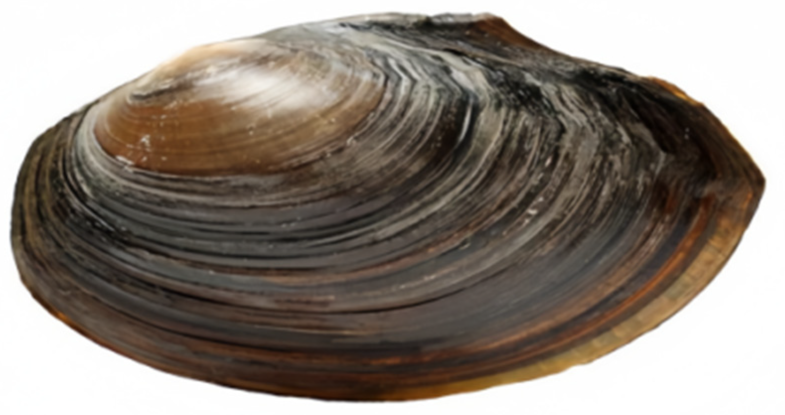
Figure 2.
Diagram of Shell Cutting.
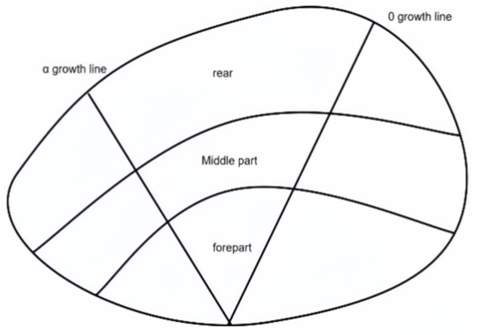
Figure 3.
Uniaxial compression test.
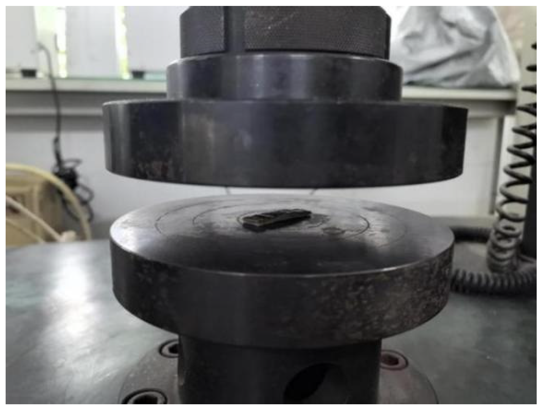
Figure 7.
Static accumulation angle test.
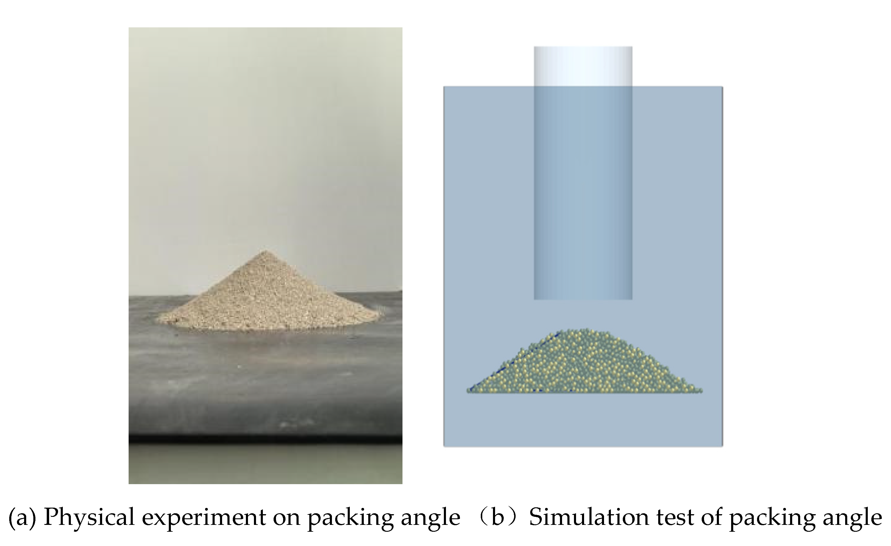
Figure 11.
Bending test simulation diagram.
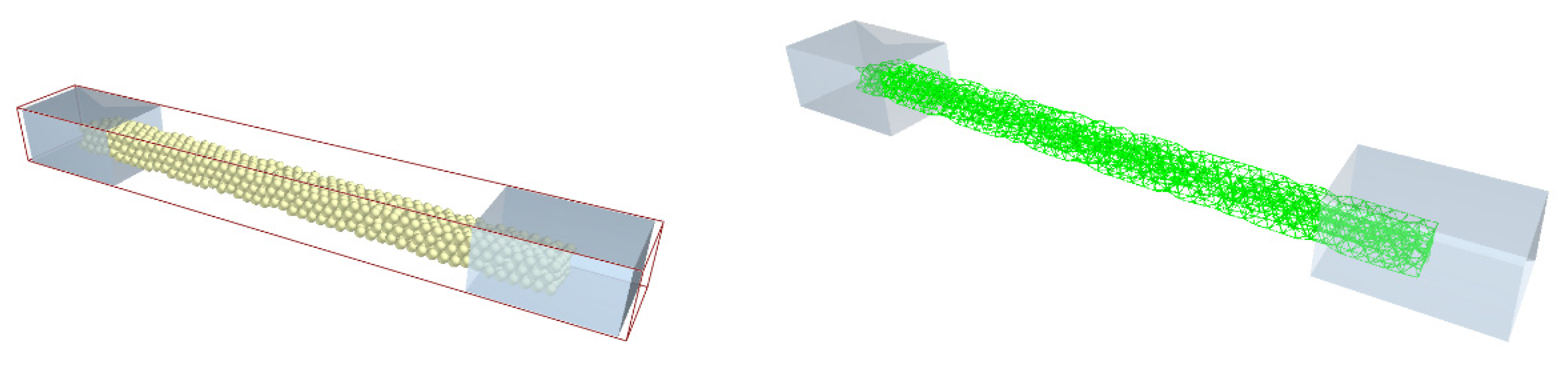
Figure 12.
Pareto Chart.
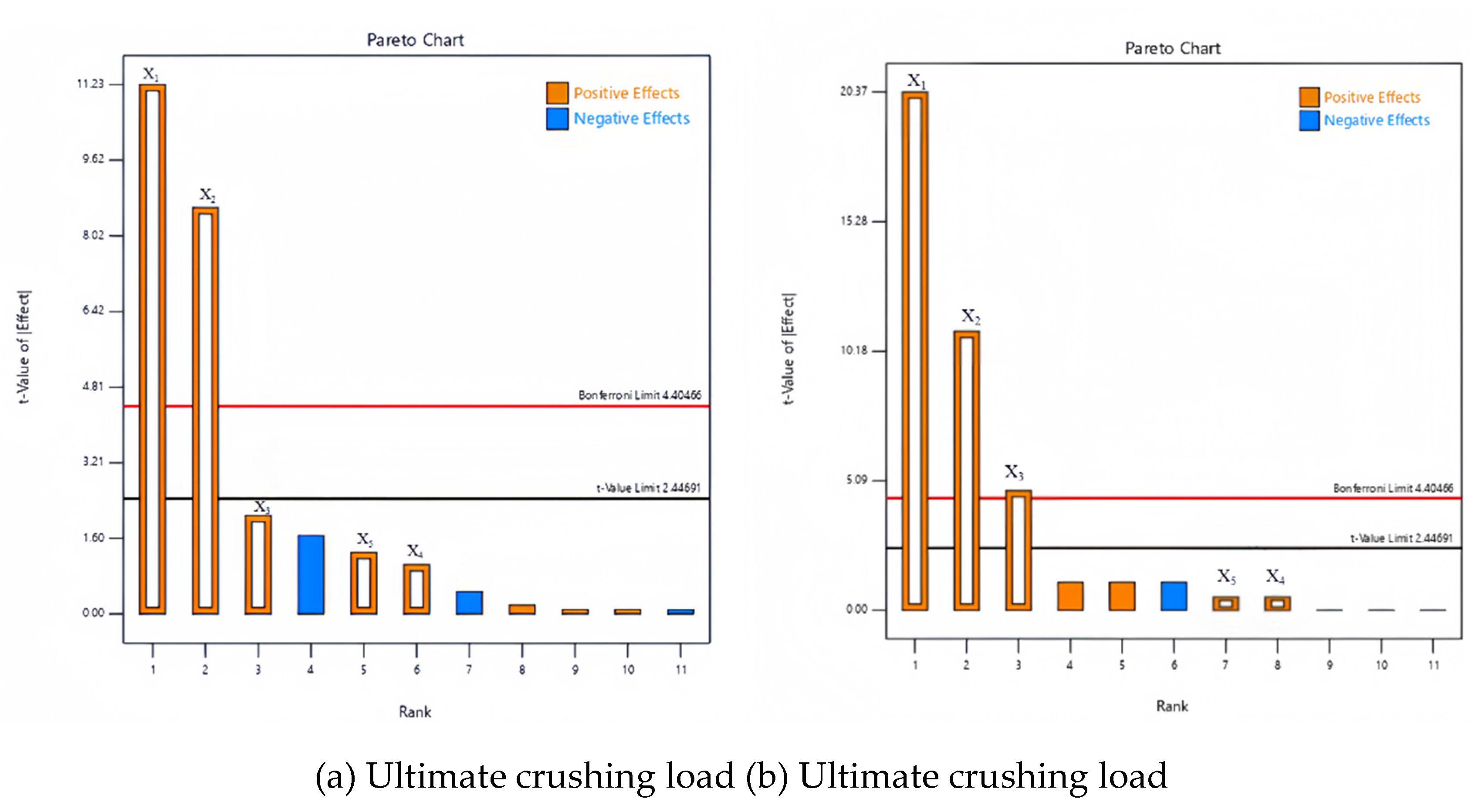
Figure 13.
Response surfaces of the interaction effects among factors for the ultimate load and ultimate displacement.
Figure 13.
Response surfaces of the interaction effects among factors for the ultimate load and ultimate displacement.
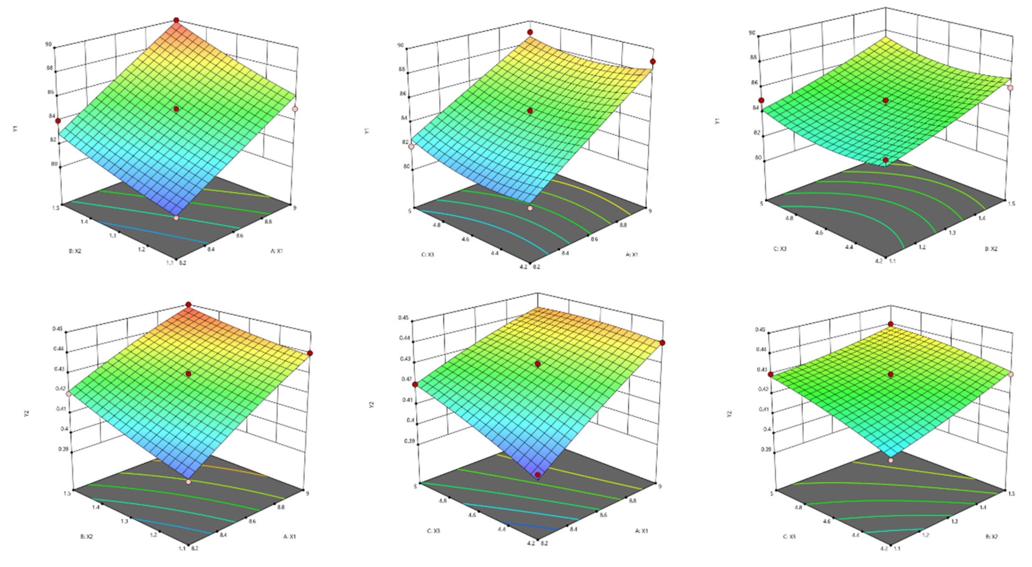
Figure 14.
Optimal combination simulation verification.
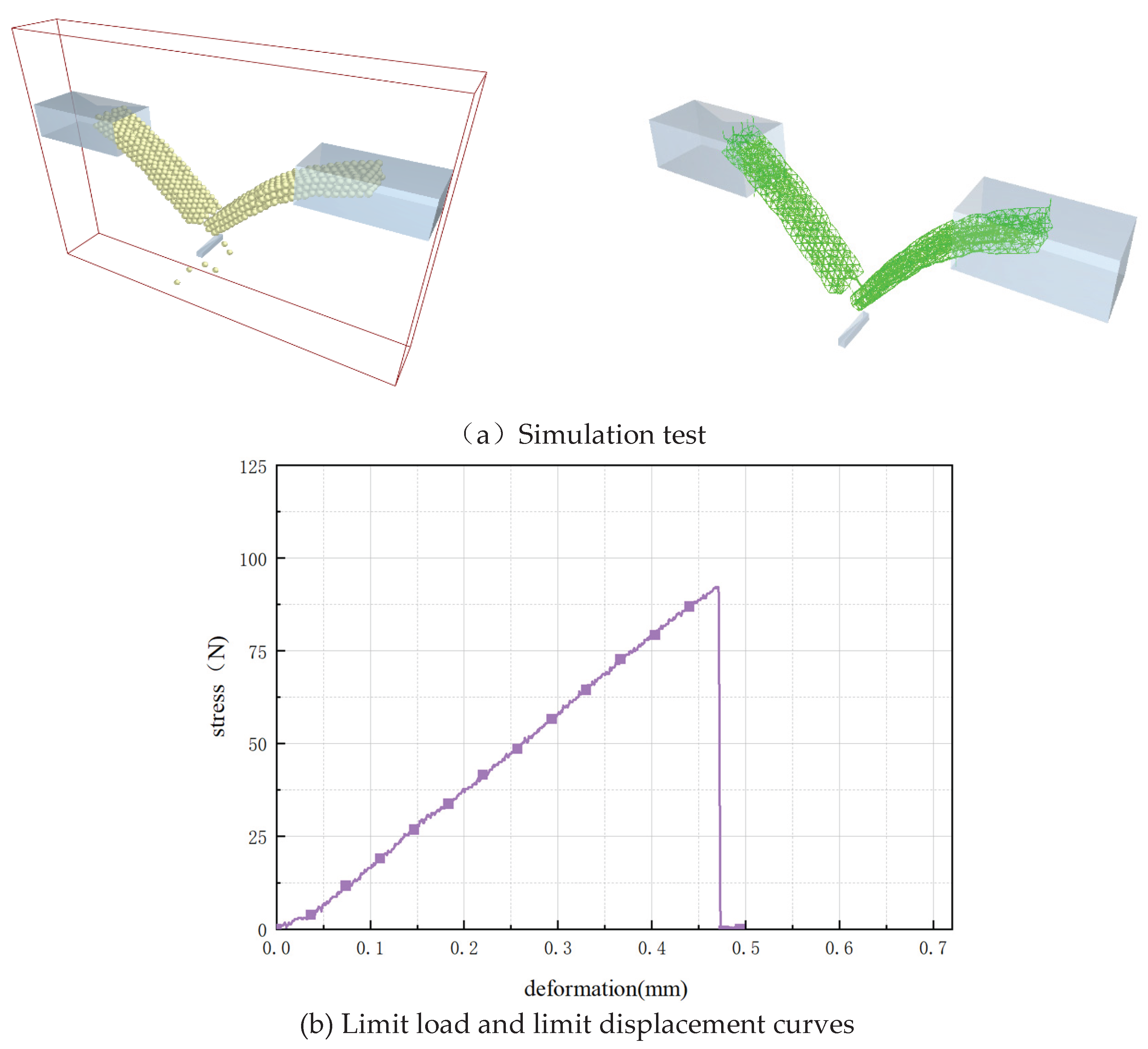

Table 1.
Plackett-Burman Experimental Factor Levels.
| Level | Factors | ||||
| X1/(N·m-3) | X2/(N·m-3) | X3/Pa | X4/Pa | X5/mm | |
| Low | 7×10¹⁰ | 5×10⁹ | 3×10⁷ | 3×10⁷ | 0.95 |
| High | 9×10¹⁰ | 1.5×10¹⁰ | 5×10⁷ | 5×10⁷ | 1.05 |
Table 2.
Results of Plackett-Burman Experiment.
| Serial Number | X1/(N·m-3) | X2/(N·m-3) | X3/Pa | X4/Pa | X5/mm | Fmax/N | Smax/mm |
| 1 | 9×10¹⁰ | 1.5×10¹⁰ | 3×10⁷ | 3×10⁷ | 0.95 | 87 | 0.44 |
| 2 | 7×10¹⁰ | 5×10⁹ | 5×10⁷ | 3×10⁷ | 1.05 | 64 | 0.36 |
| 3 | 7×10¹⁰ | 5×10⁹ | 3×10⁷ | 5×10⁷ | 0.95 | 63 | 0.34 |
| 4 | 9×10¹⁰ | 1.5×10¹⁰ | 5×10⁷ | 3×10⁷ | 0.95 | 90 | 0.45 |
| 5 | 7×10¹⁰ | 5×10⁹ | 3×10⁷ | 3×10⁷ | 0.95 | 62 | 0.34 |
| 6 | 7×10¹⁰ | 1.5×10¹⁰ | 3×10⁷ | 5×10⁷ | 1.05 | 78 | 0.39 |
| 7 | 9×10¹⁰ | 1.5×10¹⁰ | 3×10⁷ | 5×10⁷ | 1.05 | 88 | 0.45 |
| 8 | 9×10¹⁰ | 5×10⁹ | 5×10⁷ | 5×10⁷ | 1.05 | 82 | 0.42 |
| 9 | 9×10¹⁰ | 5×10⁹ | 3×10⁷ | 3×10⁷ | 1.05 | 81 | 0.40 |
| 10 | 9×10¹⁰ | 5×10⁹ | 5×10⁷ | 5×10⁷ | 0.95 | 82 | 0.42 |
| 11 | 7×10¹⁰ | 1.5×10¹⁰ | 5×10⁷ | 3×10⁷ | 1.05 | 79 | 0.39 |
| 12 | 7×10¹⁰ | 1.5×10¹⁰ | 5×10⁷ | 5×10⁷ | 0.95 | 78 | 0.39 |
Table 3.
Significance Analysis of Plackett-Burman Experiment Results.
| Source of variance | Fmax | ||||
| Sum of Squares | Degree of freedom | Mean square | F | P | |
| Model | 1014.33 | 5 | 202.87 | 41.50 | 0.0001** |
| X1 | 616.33 | 1 | 616.33 | 126.07 | <0.0001** |
| X2 | 363 | 1 | 363.00 | 74.25 | 0.0001** |
| X3 | 21.33 | 1 | 21.33 | 4.36 | 0.0817 |
| X4 | 5.33 | 1 | 5.33 | 1.09 | 0.3365 |
| X5 | 8.33 | 1 | 8.33 | 1.70 | 0.2395 |
| Residual | 29.33 | 6 | 4.89 | ||
| Total sum | 1043.67 | 11 | |||
| Source of variance | Smax | ||||
| Sum of Squares | Degree of freedom | Mean square | F | P | |
| Model | 0.0170 | 5 | 0.0034 | 111.55 | <0.0001** |
| X1 | 0.0127 | 1 | 0.0127 | 414.82 | <0.0001** |
| X2 | 0.0037 | 1 | 0.0037 | 120.27 | <0.0001** |
| X3 | 0.0007 | 1 | 0.0007 | 22.09 | 0.0033** |
| X4 | 8.333E-06 | 1 | 8.333E-06 | 0.2727 | 0.6202 |
| X5 | 8.33E-06 | 1 | 8.333E-06 | 0.2727 | 0.6202 |
| Residual | 0.0002 | 6 | 0.00000 | ||
| Total sum | 0.0172 | 11 | |||
Table 4.
Slope Climbing Test Plan and Results.
| Serial Number | X1(N·m-3) | X2(N·m-3) | X3(Pa) | Fmax(N) | Dmax(mm) | Relative error |
| 1 | 7*1010 | 5*109 | 3*107 | 64 | 0.36 | 23.4% |
| 2 | 7.4*1010 | 7*109 | 3.4*107 | 69 | 0.36 | 17.4% |
| 3 | 7.8*1010 | 9*109 | 3.8*107 | 74 | 0.37 | 11.4% |
| 4 | 8.2*1010 | 1.1*1010 | 4.2*107 | 80 | 0.4 | 4.2% |
| 5 | 8.6*1010 | 1.3*1010 | 4.6*107 | 85 | 0.43 | 1.8% |
| 6 | 9*1010 | 1.5*1010 | 5*107 | 90 | 0.45 | 7.8% |
Table 5.
BBD Test Plan and Results.
| Serial Number | X1(N·m-3) | X2(N·m-3) | X3(Pa) | Fmax/N | Smax/mm |
| 1 | 9*1010 | 1.5*1010 | 4.6*107 | 90 | 0.45 |
| 2 | 8.6*1010 | 1.3*1010 | 4.6*107 | 84 | 0.43 |
| 3 | 9*1010 | 1.1*1010 | 4.6*107 | 85 | 0.44 |
| 4 | 8.6*1010 | 1.3*1010 | 4.6*107 | 84 | 0.42 |
| 5 | 9*1010 | 1.3*1010 | 5*107 | 89 | 0.44 |
| 6 | 8.2*1010 | 1.5*1010 | 4.6*107 | 84 | 0.42 |
| 7 | 8.6*1010 | 1.5*1010 | 5*107 | 87 | 0.44 |
| 8 | 8.2*1010 | 1.3*1010 | 4.2*107 | 81 | 0.40 |
| 9 | 8.6*1010 | 1.3*1010 | 4.6*107 | 85 | 0.43 |
| 10 | 8.6*1010 | 1.1*1010 | 5*107 | 85 | 0.43 |
| 11 | 8.6*1010 | 1.3*1010 | 4.6*107 | 85 | 0.43 |
| 12 | 8.6*1010 | 1.5*1010 | 4.2*107 | 86 | 0.43 |
| 13 | 8.2*1010 | 1.3*1010 | 5*107 | 82 | 0.42 |
| 14 | 8.6*1010 | 1.3*1010 | 4.6*107 | 85 | 0.43 |
| 15 | 9*1010 | 1.3*1010 | 4.2*107 | 89 | 0.44 |
| 16 | 8.6*1010 | 1.1*1010 | 4.2*107 | 84 | 0.41 |
| 17 | 8.2*1010 | 1.1*1010 | 4.6*107 | 80 | 0.40 |
Table 6.
Analysis of Variance.
| Source of variance | Fmax | ||||||||
| Sum of Squares | Degree of freedom | Mean square | F | P | |||||
| Model | 109.55 | 9 | 12.17 | 13.21 | 0.0013** | ||||
| X1 | 84.50 | 1 | 84.50 | 91.71 | <0.0001** | ||||
| X2 | 21.12 | 1 | 21.12 | 22.93 | 0.0020** | ||||
| X3 | 1.12 | 1 | 1.12 | 1.12 | 0.3057 | ||||
| X1X2 | 0.2500 | 1 | 0.2500 | 0.2713 | 0.6185 | ||||
| X1X3 | 0.2500 | 1 | 0.2500 | 0.2713 | 0.6185 | ||||
| X2X3 | 0.0000 | 1 | 0.0000 | 0.0000 | 1.0000 | ||||
| X12 X22 X32 |
0.0105 0.1684 2.06 |
1 1 1 |
0.0105 0.1684 2.06 |
0.0114 0.1828 2.24 |
0.9179 0.6818 0.1782 |
||||
| Residual | 6.45 | 7 | 0.9214 | ||||||
| Misfitting item | 5.25 | 3 | 1.75 | 5.83 | 0.0607 | ||||
| Total sum | 116.00 | 16 | |||||||
| R2=0.9444 R2Adj=0.8729 | |||||||||
| Source of variance | Smax | ||||||||
| Sum of Squares | Degree of freedom | Mean square | F | P | |||||
| Model | 0.0030 | 9 | 0.0003 | 22.58 | 0.0002** | ||||
| X1 | 0.0021 | 1 | 0.0021 | 140.83 | <0.0001** | ||||
| X2 | 0.0004 | 1 | 0.0004 | 30.00 | 0.0009** | ||||
| X3 | 0.0003 | 1 | 0.0003 | 20.83 | 0.0026** | ||||
| X1X2 | 0.0000 | 1 | 0.0000 | 1.67 | 0.2377 | ||||
| X1X3 | 0.0001 | 1 | 0.0001 | 6.67 | 0.0364* | ||||
| X2X3 | 0.0000 | 1 | 0.0000 | 1.67 | 0.2377 | ||||
| X12 X22 X32 |
9.474E-06 4.211E-06 9.474E-06 |
1 1 1 |
9.474E-06 4.211E-06 9.474E-06 |
0.6316 0.2807 0.6316 |
0.4529 0.6126 0.4529 |
||||
| Residual | 0.0001 | 7 | 0.0000 | ||||||
| Misfitting item | 0.0000 | 3 | 8.333E-06 | 0.4167 | 0.7510 | ||||
| Total sum | 0.0032 | 16 | |||||||
| R2=0.9667 R2Adj=0.9239 | |||||||||
Disclaimer/Publisher’s Note: The statements, opinions and data contained in all publications are solely those of the individual author(s) and contributor(s) and not of MDPI and/or the editor(s). MDPI and/or the editor(s) disclaim responsibility for any injury to people or property resulting from any ideas, methods, instructions or products referred to in the content. |
© 2025 by the authors. Licensee MDPI, Basel, Switzerland. This article is an open access article distributed under the terms and conditions of the Creative Commons Attribution (CC BY) license (http://creativecommons.org/licenses/by/4.0/).
Copyright: This open access article is published under a Creative Commons CC BY 4.0 license, which permit the free download, distribution, and reuse, provided that the author and preprint are cited in any reuse.


