
Submitted:
25 November 2025
Posted:
26 November 2025
You are already at the latest version
Abstract
To solve the problem of insufficient joint tracking performance in the feedforward control of industrial robots caused by model and control quantity errors, a data-driven feedforward optimization algorithm is proposed. This algorithm not only enhances joint tracking performance but also optimizes trajectory accuracy. Firstly, aiming at the nonlinear residuals in the dynamic model resulting from linear assumptions, neglect of high-order terms and other factors, a joint torque residual fitting method based on ensemble learning is proposed. This method constructs a hybrid dynamic model that combines mechanism-based and data-driven approaches, thereby improving the accuracy of torque feedforward quantities. Secondly, based on the principle of iterative learning control, a data-driven velocity feedforward optimization algorithm is proposed. By comparing historical and real-time data, the learning gain is dynamically adjusted, and the velocity feedforward parameters are updated iteratively to reduce joint tracking deviations. Finally, experiments on industrial robot verify that the torque residual fitting based on ensemble learning reduces the joint torque prediction error by more than 77%. After optimizing the feedforward control quantities, the root mean square error of joint tracking is significantly improved: it is reduced by more than 60% for linear trajectories and by more than 20% for circular trajectories.
Keywords:
feedforward control
; ensemble learning
; iterative learning control
; data-driven
; industrial robot
1. Introduction
In typical application scenarios such as welding, cutting and machining, industrial robots are subject to motion constraints from the environment or processing tasks. They must not only ensure that the end-effector reaches the target pose accurately but also maintain that the trajectory tracking accuracy throughout the motion meets process standards [1,2]. Independent joint PID control is widely used due to its simple structure and ease of engineering implementation. This method achieves trajectory tracking through closed-loop control of each joint [3,4]. However, this control strategy designed for linear time-invariant systems suffers from insufficient dynamic responsiveness and fails to accommodate the nonlinear time-varying characteristics of robot systems [5].
To further improve trajectory tracking performance, researchers have turned to control strategies based on dynamic models, mainly forming two typical schemes [6]: One is robot model dynamic compensation control, which constructs an inner control loop to real-time compensate for the nonlinear dynamic characteristics of the system, decoupling the complex robot system into approximately linear and controllable objects easily; the other is robot dynamic model feedforward control, which predicts the system motion state based on an accurate dynamic model, pre-compensates dynamic terms through a feedforward path, and forms a composite control architecture with feedback control. Compared with model-based dynamic compensation control, the core advantage of feedforward control lies in taking high-quality desired motion commands as input, predicting and compensating via a dynamic model, and addressing real-time computation issues through strategies such as pre-storing compensation terms [7]. Chen [8] decomposes real-time position tracking errors effectively through feedforward control based on a dynamic model, and uses various proportional-derivative controllers and their adaptive versions to calculate real-time compensation torque for different position tracking errors, so as to achieve fast response and stability of the control system. However, such methods have high requirements for the accuracy of system models and parameters, and disturbances caused by internal uncertain disturbances of the robot will affect the control effect of the algorithm. Jia [9] analyzes the nonlinear characteristics of joint torque through chaos theory based on a chaotic regression tree dynamic model, and performs torque feedforward compensation based on these characteristics to suppress vibration during low-speed movement of the robot and improve trajectory tracking accuracy. Song [10] proposes a dynamic velocity feedforward compensation control method based on radial basis function neural network (RBF-NN). The feedforward generator takes the robot's mechanism dynamic model as the basis of the accurate dynamic model, and identifies uncertain parts online through RBF-NN to improve dynamic modeling accuracy. However, most feedforward strategies focus on torque feedforward and position feedforward, while neglecting the impact of velocity feedforward on control performance [11,12,13,14].
When robots perform the same or similar tasks repeatedly, iterative learning control can implement optimal feedforward control through learning [15]. There are mainly two ways to optimize feedforward control: One is to directly tune the feedforward control quantity [16], which fits the iterative learning control signal through the least square method to tune the acceleration and jerk feedforward, uses various search algorithms to determine the structure of the model-based feedforward controller, and then optimizes its parameters by fitting the iterative learning control signal with the least square method to compensate for residual tracking errors, so as to achieve efficient tuning of the feedforward controller for precision motion systems. The other is to tune the parameters of the feedforward control filter [17], which obtains the optimal feedforward control quantity through iterative learning control, determines the globally optimal parameters of the feedforward controller with a filter by combining the linear least square method, and uses the stable approximation method of the zero-phase error tracking algorithm to solve its stability problem, so as to achieve high tracking performance for repeated and varying tasks. Both schemes facilitate the optimization of feedforward parameters through system dynamic characteristic information.
Aiming at the problem of joint tracking performance of industrial robots, this paper proposes a data-driven feedforward control optimization strategy. In section 2, the shortcomings of the general feedforward structure are analyzed, and the feedforward generator structure proposed in this paper is presented. In section 3, a joint torque residual model learning method based on ensemble learning is proposed to construct a hybrid dynamic model combining a mechanism model and a data-driven model, so as to improve the accuracy of torque feedforward control quantity. In section 4, a velocity feedforward control optimization algorithm based on the principle of iterative learning control is proposed to adjust the learning gain of velocity feedforward dynamically and improve the tracking deviation gradually caused by insufficient joint tracking performance. In section 4, experiments on torque residual fitting and feedforward quantity optimization are completed based on the proposed algorithm. The effectiveness of the proposed algorithm is verified by comparing indicators such as torque residual, tracking error and trajectory accuracy before and after optimization.
2. Data-Driven Feedforward Generator
The structure of the industrial robot control system is shown in Figure 1.
Conventional servo controllers are designed for linear time-invariant systems and only focus on position-level control, without involving the decoupling of robot dynamic characteristics. Large inertia changes may cause system oscillations, resulting in large tracking errors at the end-effector of the manipulator. Therefore, feedforward control quantities are introduced into the velocity loop and current loop to address the nonlinear time-varying issues. A typical robot feedforward generator obtains the theoretical joint torque through the robot inverse dynamics equation based on joint position, velocity and acceleration. The torque feedforward control quantity and velocity feedforward control quantity are obtained by applying low-pass filtering to the theoretical joint torque and the velocity feedforward term respectively.
During the actual operation of the robot, affected by factors such as robot load changes, nonlinear characteristics and servo tracking performance, the residual between the actual joint torque and the theoretical torque cannot be ignored. If the theoretical torque is used as the feedforward control quantity directly, it will have an adverse impact on the control effect. For the velocity feedforward control quantity, it will degrade the control performance, such as increasing joint tracking errors. However, due to the complexity of robot motion, the required gains may vary under different working conditions. If the gain is selected improperly, it will not only reduce the joint tracking performance but may even cause vibration due to tracking overshoot.
From the analysis of the shortcomings of the feedforward generator, it can be concluded that improving the accuracy of the robot dynamic model and optimizing the velocity feedforward gain can enhance the feedforward effect, thereby improving the joint tracking performance. The data-driven joint feedforward generator designed in this paper is shown in Figure 2.
The data-driven feedforward generator adds a process data storage area, which records the position error , velocity error and torque error during the joint movement process, as well as the feedforward control quantities and adopted each time under the same trajectory. This paper will use a data-driven method to improve the feedforward control effect.
3. Torque Feedforward Optimization Algorithm Based on Ensemble Learning
The joint torque feedforward control quantity is calculated via inverse dynamics using the joint planned position, velocity and acceleration, as shown in (1):
where denotes the robot dynamic model function, and represents the dynamic parameters.
Although the identified parameters enable real-time calculation of joint torques, complex disturbances during robot operation, such as frictional nonlinearity, motor cogging effect, and control signal quantization error, result in a significant discrepancy between the torques predicted by the dynamic model and the actual joint torques [18]. This error not only reduces the model's prediction accuracy but also impairs the performance of feedforward control directly.
3.1. Data-Driven Torque Feedforward Generator
Given the typical characteristic of industrial robots performing periodic and repetitive tasks, sequence modeling methods such as Recurrent Neural Network (RNN), Long Short-Term Memory (LSTM), and Temporal Convolutional Network (TCN) have been widely used to model torque residuals during trajectory operation. By collecting historical data under the same trajectory, researchers employ regression analysis or neural network algorithms to construct a residual prediction model, thereby enhancing the torque prediction accuracy of the robot’s dynamic model.
In response to the nonlinear residuals existing in the calculation of the mechanism model, this paper trains residual models for each joint through a data-driven approach. During actual operation, the dynamic residuals are predicted by the model, and finally the hybrid model joint torque is obtained to improve the accuracy and robustness of the dynamic model. The underlying principle is shown in Figure 3.
Thus, the final torque feedforward control quantity is obtained as:
where is the residual model obtained through training, and is the input feature of the model.
3.2. Joint Torque Residual Fitting Based on Ensemble Learning
Since the robot controller data and servo driver data obtained through the communication interface are non-real-time, the available collected data exist as sparse time series in tabular form. The prediction accuracy of sequence modeling methods based on Deep Neural Networks (DNNs) relies on a single neural network, and unreasonable model structures and hyperparameters can lead to overfitting or underfitting easily [19]. Compared with single neural network methods, ensemble learning constructs a strong learner with higher accuracy and generalization ability by integrating multiple base learners. The integration and training mechanism of base learners can reduce the risk of overfitting. There are three main paradigms of ensemble learning, including Bagging, Boosting and Stacking. XGBoost is an ensemble learning model based on the Boosting paradigm, which uses Classification and Regression Trees (CART) as base learners. For the residual prediction task in this study, XGBoost has multiple advantages over DNNs:
1. Tabular data processing capability: XGBoost is more suitable for processing tabular data than DNNs in terms of accuracy and stability [20]. DNNs are better at capturing multi-dimensional data features through spatiotemporal position modeling, while XGBoost has superior fitting ability for structured tabular data.
2. Adaptability to sparse data: XGBoost is designed with a sparsity-aware algorithm to guide node splitting in tree learning, enabling it to perform better when processing sparse data [20]. This feature is highly compatible with the input characteristics of the sparse time series in this paper.
Therefore, this paper adopts the XGBoost learning method to construct the joint residual model. For a given dataset , where denotes the feature vector of the i-th sample, is the corresponding label, and represent the number of samples and the number of features respectively, the XGBoost model can be expressed as:
where represents the input data, denotes the predicted value, is the number of CART trees in the XGBoost model, stands for the predicted value of the k-th tree for , denotes the function space of CART, is the structure of each tree, T is the number of leaf nodes, and each corresponds to an independent tree structure and leaf weight . XGBoost establishes tree structures by minimizing the following regularized objective function:
where is the loss function term, which characterizes the error between and , and , is the regularization term, a penalty term for model complexity that helps avoid overfitting. XGBoost realizes training by iteratively adding trees. During the t-th iteration, the predicted value of the i-th sample can be expressed as:
where represents the predicted value from the (t-1)-th iteration. Finally, a greedy algorithm is employed for tree branching. Starting from a single leaf node, split points are iteratively added to split leaf nodes and form branches, ultimately forming the tree structure.
4. Iterative Learning-based Velocity Feedforward Optimization Algorithm
As shown in the schematic diagram of the feedforward controller, robot dynamic parameters, motor control system parameters, filter parameters, etc., form a complex system. Errors in these parameters will prevent model-based optimization algorithms from obtaining optimal solutions.
4.1. Data-Driven Velocity Feedforward Generator
Treating the current loop as the controlled object G, the robot joint control system is simplified as shown in Figure 4. In the diagram, represents the joint control input, denotes the system output, E is the difference between the output and the input, F stands for the feedforward control transfer function, and C1 is the feedback controller transfer function.
As can be seen from the diagram, the transfer function of the system tracking error is:
It can be concluded that the goal of velocity feedforward optimization is to make the tracking error zero, i.e.:
Since is a continuous function within the effective interval, according to Weierstrass's First Approximation Theorem [21], can be approximately expressed as:
where is the parameter of the -th order system.
In an ideal scenario, if the feedforward parameters meet the requirements of (8), the control error can be reduced to zero. However, such an ideal situation occurs rarely in practical applications. In view of the difference between the actual situation and the ideal state, this paper adopts the iterative learning method for parameter design, and updates the velocity feedforward control quantity gradually through a continuous iterative learning process, as shown in (9):
4.2. Parameter Optimization Based on Iterative Learning
For the tracking error of joint i at a certain moment, the feedforward control function of the k-th iteration is defined as:
where denotes the parameter of the l-th order control quantity in the k-th iteration.
The joint velocity tracking error of joint i obtained in the k-th iteration is given by:
where is the reference of joint i in the S-domain, is the observation of joint i in the S-domain.
By performing the inverse Laplace transform on (11), the time-domain error is obtained:
where denotes the j-th order derivative of the target position of joint i with respect to time, represents the j-th order derivative of the actual position of joint i in the k-th iteration, is the theoretical parameter vector of the joint i system, and is the feedforward parameter vector of joint i in the k-th iteration.
The first-order Taylor expansion of the tracking error of joint i at is:
where is the Jacobian matrix of joint i with respect to the feedforward parameters, as (14):
Thus, the iterative formula of the feedforward parameters is obtained as (15), which is derived based on the analysis of tracking error at a specific moment and the iterative algorithm:
To minimize the tracking error of the entire trajectory during joint movement, it is necessary to minimize the sum of tracking errors at all sampling moments along the trajectory. For a given trajectory, this section defines the iterative optimization objective of the feedforward control quantity as:
where and are the target position and actual position of joint i at the j-th sampling moment respectively. It can be concluded that the Jacobian matrix for the entire trajectory is:
Therefore, the strategy adopted in this paper is: for each joint, optimize a set of parameters to minimize the trajectory optimization objective (16). Finally, the iterative formula for the feedforward parameters is obtained as:
5. Experimental Verification and Result Analysis
Experiments on torque residual fitting and feedforward iterative optimization were conducted on the platform shown in Figure 5.
The robot employed in the experiments was a SIASUN T12B 6-axis industrial robot, with a rated load of 14 kg and a maximum workspace reach of 1465 mm. To verify the robot's tracking performance, a rated load was installed at the end-effector. The actual torque of each joint was obtained from the corresponding servo driver. The experimental trajectories included a linear trajectory with a length of 1400 mm and a circular trajectory with a radius of 100 mm, and the target trajectory speed of the end-effector was 1.5 m/s.
5.1. Torque Residual Fitting Experiment
During the robot's actual operation, multi-joint synchronous motion is required, and the mutual influence between joints makes the joint torque residual more significant. The dynamic model identification was completed using the parameter identification algorithm [22], and the robot was controlled to complete the circular experimental trajectory to obtain the characteristic values, as shown in Figure 6. It reveals that due to the load and inter-joint coupling effects, the RMSE of each joint’s torque residual is significantly larger than that of the torque residual from the parameter identification verification trajectory.
The joint position, velocity, acceleration, theoretical torque, and actual torque from Figure 6 were used as the model inputs, while the residual torque was used as the model output to train the joint residual model. The hyper-parameters of the fitting model are shown in Table 1.
Subsequently, the model was downloaded to the robot controller, and the same trajectory was run to obtain the residual torque predicted by the model. The sum of the theoretical torque and the predicted residual torque constitutes the final predicted torque, as shown in Figure 7. In the experiment, the training time for the single-joint residual model was 0.5 seconds, and the time consumed by the model for torque prediction in the robot controller was less than 20 microseconds.
Table 2 presents the RMSE of the torque residuals between the theoretical torque based on the mechanism model and the final predicted torque based on the hybrid model. It can be seen from the table that the predicted torque errors of all joints obtained based on ensemble learning are significantly improved: the maximum improvement rate reaches 93.865%, the minimum improvement rate is 77.595%, and the average reduction rate of errors is 84.808%.
From the experimental results, it can be concluded that the torque residual fitting based on ensemble learning can significantly improve the accuracy of joint predicted torque. It is applicable to both single-joint motion and multi-joint synchronous motion. Moreover, it consumes less time in training and real-time operation, serving as a fundamental basis for precise torque feedforward control.
5.2. Feedforward Control Quantity Optimization Experiment
After completing the joint torque fitting, the feedforward control quantity optimization was performed for both linear and circular test trajectories. In the linear test trajectory experiment, the learning process converged and terminated after 2 torque feedforward iterations and 2 velocity feedforward iterations. The curves of the differences between the actual joint angles and theoretical angles for each iteration are plotted in Figure 8. It can be seen from the figure that due to the accurate dynamic modeling in this paper, the optimization of the torque feedforward control quantity has little impact on improving trajectory tracking performance, while velocity feedforward learning contributes a larger proportion of the optimization effect.
In the circular trajectory experiment, the learning process converged and terminated after 1 torque feedforward iteration and 2 velocity feedforward iterations. The curves of the differences between the actual joint angles and theoretical angles for each iteration are plotted in Figure 9. It can be seen from the figure that compared with the linear trajectory, the circular trajectory has fewer high-speed segments on the joint side, and the tracking error amplitude before optimization is smaller, thus the overall improvement ratio is relatively lower. However, the position tracking error amplitude of each joint is consistent with that of the linear trajectory, indicating that the optimization effect is consistent across different trajectory types.
The optimization results of the above two experiments are shown in Table 3. From the experimental data, it can be seen that the optimization algorithm proposed in this paper can achieve excellent performance improvement with fewer than 4 iterations. It exhibits good convergence speed and optimization effect. After iterative learning, the tracking RMSE of each joint for the linear trajectory is improved by more than 60%, and that for the circular trajectory is improved by more than 20%, making it suitable for typical robot trajectories.
Based on the feedforward control quantity optimization results, the theoretical trajectory, pre-optimization trajectory, and post-optimization trajectory were calculated using the actual joint values obtained before and after optimization, as shown in Figure 10. It can be seen from the figure that due to the improved joint tracking performance, the trajectory straightness of the robot during high-speed linear motion is significantly enhanced. When the robot performs circular motion, since the joint displacement is small and the speed is low, the trajectory error is not mainly caused by joint tracking deviation.
The trajectory optimization data are presented in Table 4. For the linear trajectory, the average error is reduced by 72.268% after optimization; the maximum error mainly originates from the tracking deviation in the start and end segments, and this maximum error is reduced by 64.831% after optimization. For the circular trajectory, the average error and maximum error are reduced by 3.78% and 13.517%, respectively.
From the experimental results, it can be concluded that the feedforward optimization algorithm proposed in this paper can improve the accuracy of joint trajectory tracking and robot end-effector trajectory effectively.
6. Discussion
This paper proposes a data-driven feedforward control optimization method for industrial robots. This method uses an ensemble learning algorithm to fit joint torque residuals, thereby improving the accuracy of the dynamic model. Additionally, it adopts the principle of iterative learning control to dynamically adjust the velocity feedforward gain by comparing historical and real-time data, thus enhancing joint tracking performance. Experimental results demonstrate that optimizing the feedforward control quantities significantly improves the joint tracking RMSE: the reduction exceeds 60% for linear trajectories and 20% for circular trajectories. Meanwhile, the trajectory precision is significantly enhanced, with the maximum error decreasing by 64.83% for linear trajectories and 13.52% for circular trajectories.
Author Contributions
Conceptualization, L.L.; software, L.L.; validation, L.L.; writing—original draft preparation, L.L.; writing—review and editing, L.L; supervision, C.W.; project administration, C.W. All authors have read and agreed to the published version of the manuscript.
Funding
This research was funded by Major Special Project of Innovation Consortium, grant number 2023JH1/11200014.
Institutional Review Board Statement
Not applicable.
Informed Consent Statement
Informed consent was obtained from all subjects involved in the study.
Data Availability Statement
The experimental data and code related to this article can be accessed via the following link: https://github.com/FantasyRobot/Data-Driven-Feedforward-Optimization-Algorithm-for-Indus-trial-Robots.
Conflicts of Interest
The authors declare no conflicts of interest.
References
- Zhang, Y.; Jiang, Y.; Tian, X.; Xu, X.; et al. A Point Cloud-Based Welding Trajectory Planning Method for Plane Welds. Int. J. Adv. Manuf. Technol. 2023, 125, 1645–1659. [Google Scholar] [CrossRef]
- Peng, J.; Ding, Y.; Zhang, G.; Ding, H. Smoothness-Oriented Path Optimization for Robotic Milling Processes. Sci. China Technol. Sci. 2020, 63, 1751–1763. [Google Scholar] [CrossRef]
- Vasu, S. Fuzzy PID Based Adaptive Control on Industrial Robot System. Mater. Today Proc. 2018, 5, 13055–13060. [Google Scholar]
- Wang, J.; Zhu, Y.; Qi, R.; Zheng, X.; et al. Adaptive PID Control of Multi-DOF Industrial Robot Based on Neural Network. J. Ambient Intell. Humaniz. Comput. 2020, 11, 6249–6260. [Google Scholar] [CrossRef]
- Tinoco, V.; Silva, M.F.; Santos, F.N.; Morail, R.; et al. A Review of Advanced Controller Methodologies for Robotic Manipulators. Int. J. Dyn. Control 2025, 13, 36. [Google Scholar] [CrossRef]
- Yuan, M.; Manzie, C.; Good, M.; Shames, I.; et al. A Review of Industrial Tracking Control Algorithms. Control Eng. Pract. 2020, 102, 104536. [Google Scholar] [CrossRef]
- Liu, L.; Tian, S.; Xue, D.; Zhang, T.; et al. Industrial Feedforward Control Technology: A Review. J. Intell. Manuf. 2019, 30, 2819–2833. [Google Scholar] [CrossRef]
- Chen, L.; Ling, S.; Chen, T.; Cai, Y.; et al. Improved Torque Feedforward Compensation Method Considering Position Tracking Error Compensation. Ind. Robot 2025, 52, 5. [Google Scholar] [CrossRef]
- Jia, B.; Chen, L.; Zhang, L.; Fu, Y.; et al. Vibration Suppression of Welding Robot Based on Chaos-Regression Tree Dynamic Model. Nonlinear Dyn. 2024, 112, 4393–4407. [Google Scholar] [CrossRef]
- Song, W.; Xiao, J.; Wang, G.; Wang, G. Dynamic Velocity Feed-Forward Compensation Control with RBF-NN System Identification for Industrial Robots. Trans. Tianjin Univ. 2013, 19, 118–126. [Google Scholar] [CrossRef]
- Wang, C.; Zhao, S.; Zheng, T.; et al. An Adaptive Feedforward Optimization Mechanism for Improving Industrial Robots Trajectory Tracking Performance through Iterative Learning. In Proceedings of the 2025 9th International Conference on Robotics, Control and Automation (ICRCA ), Shanghai, China, 10 January 2025. [Google Scholar]
- Pizarro-Lerma, A.; Santibañez, V.; Garcia-Hernandez, R.; et al. A New Motion Tracking Controller with Feedforward Compensation for Robot Manipulators Based on Sectorial Fuzzy Control and Adaptive Neural Networks. Mathematics 2025, 13, 977. [Google Scholar] [CrossRef]
- Li, B.; Zhang, W.; Li, Y.; et al. Positional Accuracy Improvement of an Industrial Robot Using Feedforward Compensation and Feedback Control. J. Dyn. Syst. Meas. Control 2022, 144, 071003. [Google Scholar] [CrossRef]
- Zhou, R.; Hu, C.; Hou, B.; et al. Comparative Study of Performance-Oriented Feedforward Compensation Strategies for Precision Mechatronic Motion Systems. IEEE Access 2022, 10, 100812–100823. [Google Scholar] [CrossRef]
- Bristow, D.A.; Tharayil, M.; Alleyne, A.G. Real-Time Iterative Learning Control: Design and Applications, 1st ed.; Springer: London, UK, 2009; pp. 7–27. [Google Scholar]
- Dai, L.; Li, X.; Zhu, Y.; Zhang, M. Feedforward Tuning by Fitting Iterative Learning Control Signal for Precision Motion Systems. IEEE Trans. Ind. Electron. 2020, 68, 8412–8421. [Google Scholar] [CrossRef]
- Zhang, X.; Li, M.; Ding, H.; Yao, X. Data-Driven Tuning of Feedforward Controller Structured with Infinite Impulse Response Filter via Iterative Learning Control. IET Control Theory Appl. 2019, 13, 1062–1070. [Google Scholar] [CrossRef]
- Sciavicco, L.; Siciliano, B. Modeling, Identification and Control of Robots, 1st ed.; Hermes Penton: London, UK, 2002. [Google Scholar]
- Deng, J.; Ni, H.; Ji, S.; Liang, L.; et al. Hybrid Friction Modeling Method for Robot Joints Integrating Mechanistic Model and Ensemble Learning. Chin. J. Eng. 2024, 46, 1140–1150. [Google Scholar]
- Chen, T.; Guestrin, C. XGBoost: A Scalable Tree Boosting System. In Proceedings of the 22nd ACM SIGKDD International Conference on Knowledge Discovery and Data Mining, San Francisco, CA, USA, 13–17 August 2016. [Google Scholar]
- Pinkus, A. Weierstrass and Approximation Theory. J. Approx. Theory 2000, 107, 1–66. [Google Scholar] [CrossRef]
- Liang, L.; Wu, C.; Liu, S. A Terminal Residual Vibration Suppression Method of a Robot Based on Joint Trajectory Optimization. Machines 2024, 12, 537. [Google Scholar] [CrossRef]
Figure 1.
Block diagram of robot control system.
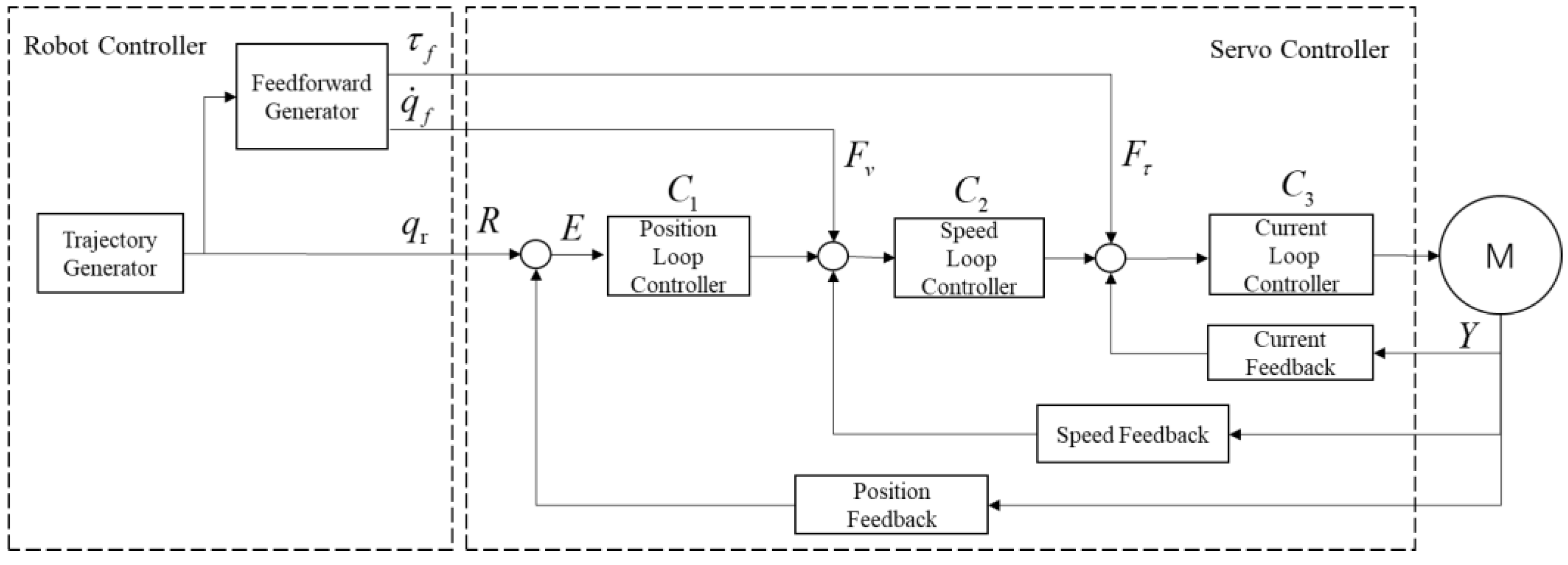
Figure 2.
Block diagram of data-driven feedforward generator.
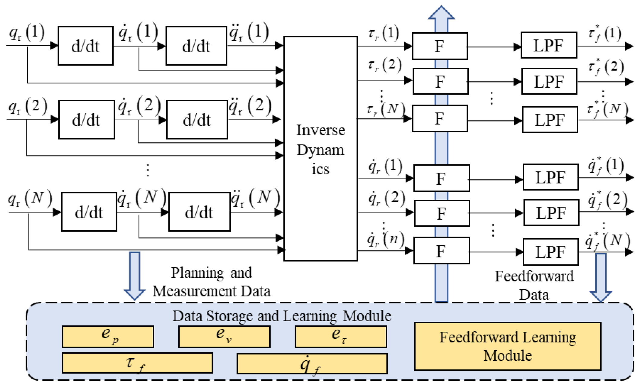
Figure 3.
Block diagram of joint torque calculation based on hybrid model.
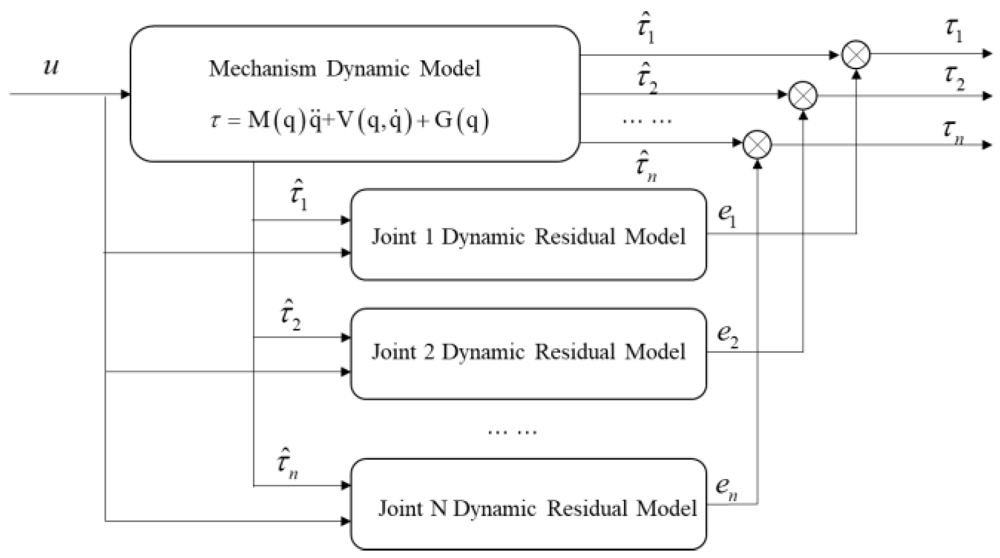
Figure 4.
Simplified block diagram of robot joint control system.
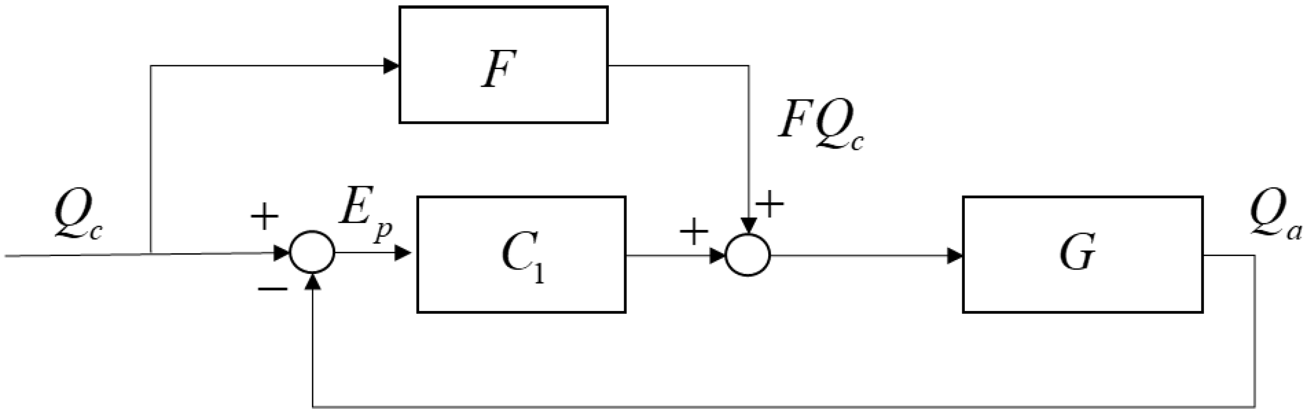
Figure 5.
Experimental platform and trajectory. (a) SIASUN T12B robot, (b) linear trajectory, (c) circular trajectory.
Figure 5.
Experimental platform and trajectory. (a) SIASUN T12B robot, (b) linear trajectory, (c) circular trajectory.
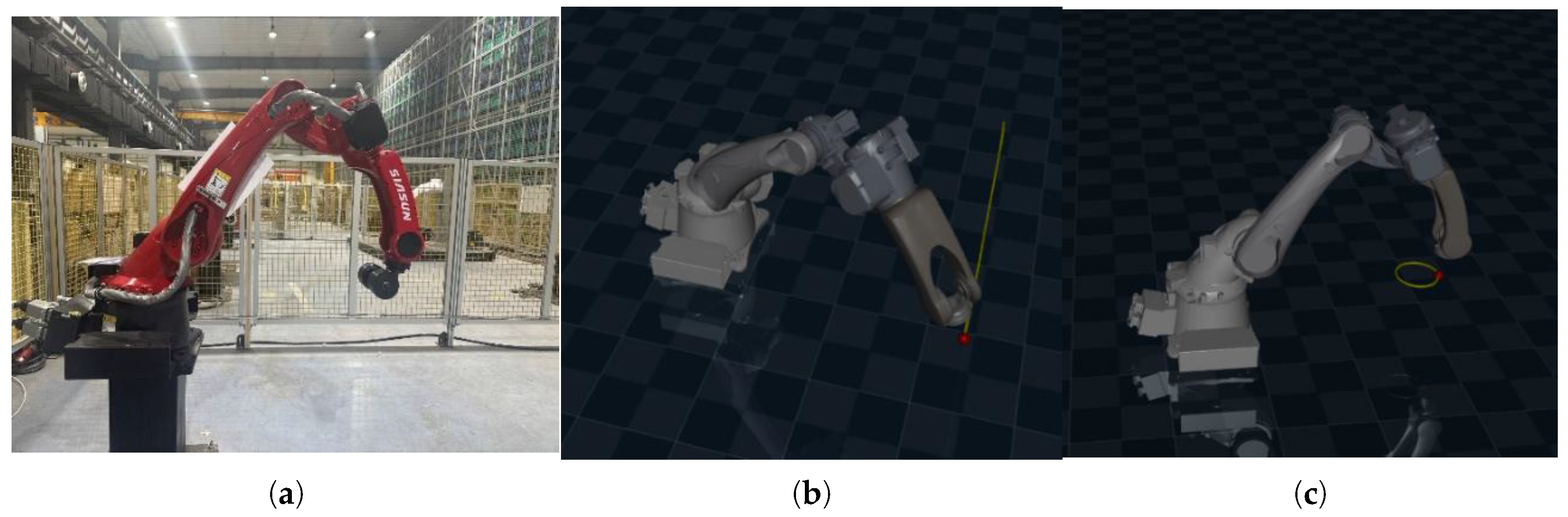
Figure 6.
Feature data curves of each joint. (a) position curve, (b) speed curve, (c) acceleration curve, (d) theoretical torque curve, (e) actual torque curve, (f) residual torque curve.
Figure 6.
Feature data curves of each joint. (a) position curve, (b) speed curve, (c) acceleration curve, (d) theoretical torque curve, (e) actual torque curve, (f) residual torque curve.
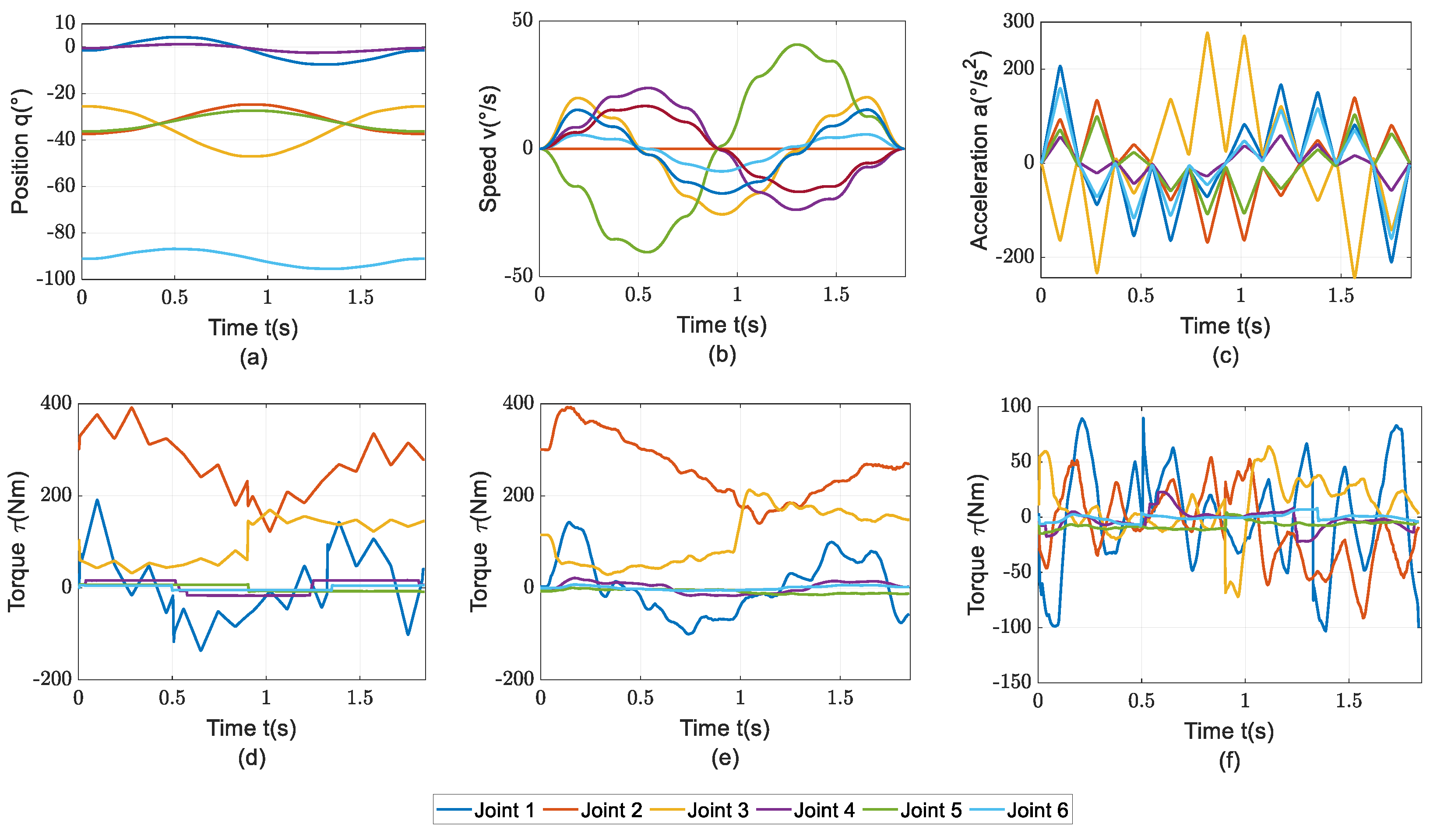
Figure 7.
Difference between predicted and actual torque. (a) residual of joint 1, (b) residual of joint 2, (c) residual of joint 3, (d) residual of joint 4, (e) residual of joint 5, (f) residual of joint 6.
Figure 7.
Difference between predicted and actual torque. (a) residual of joint 1, (b) residual of joint 2, (c) residual of joint 3, (d) residual of joint 4, (e) residual of joint 5, (f) residual of joint 6.
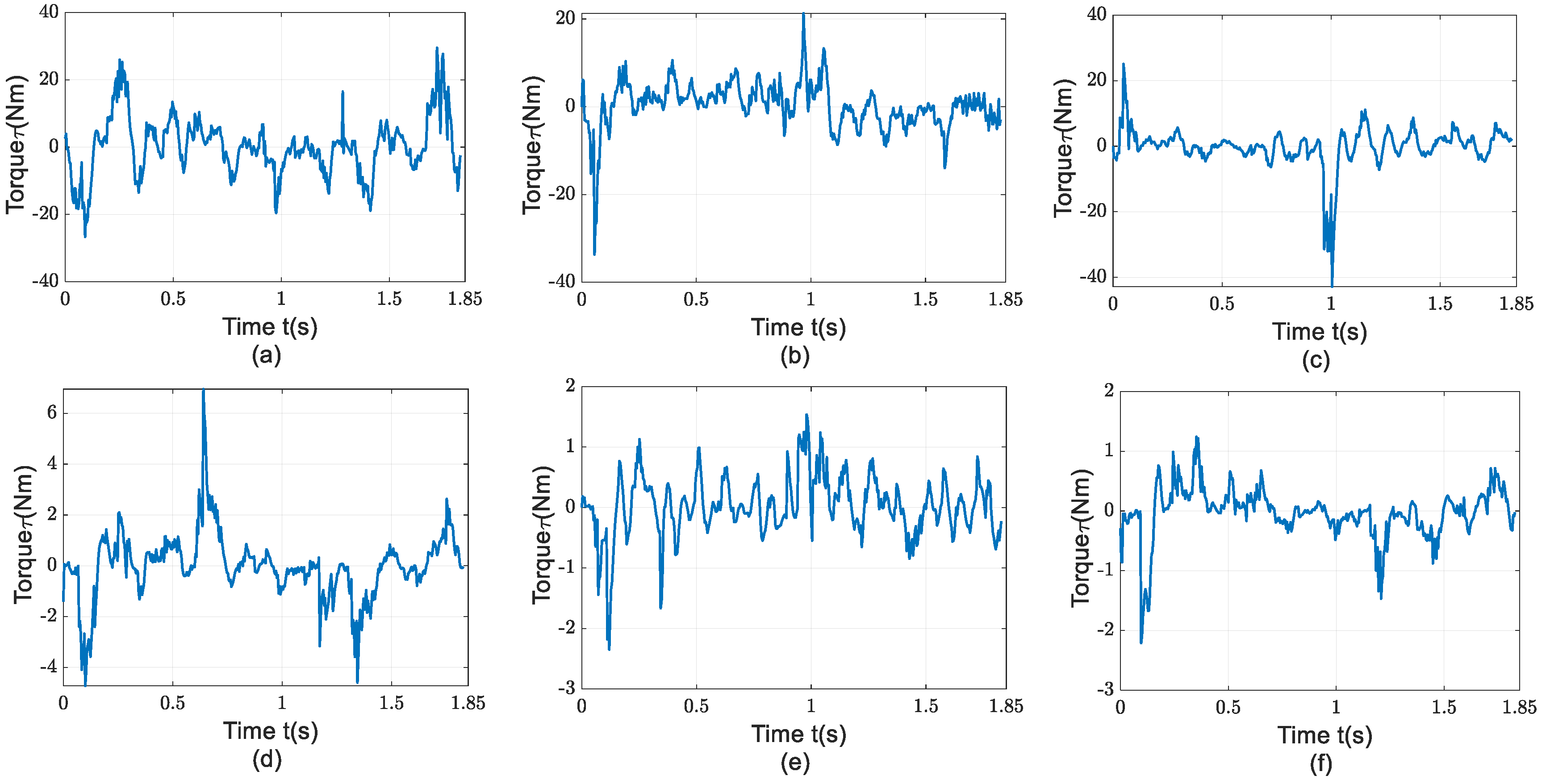
Figure 8.
Joint tracking error curves for linear trajectory. (a) error of joint 1, (b) error of joint 2, (c) error of joint 3, (d) error of joint 4, (e) error of joint 5, (f) error of joint 6.
Figure 8.
Joint tracking error curves for linear trajectory. (a) error of joint 1, (b) error of joint 2, (c) error of joint 3, (d) error of joint 4, (e) error of joint 5, (f) error of joint 6.
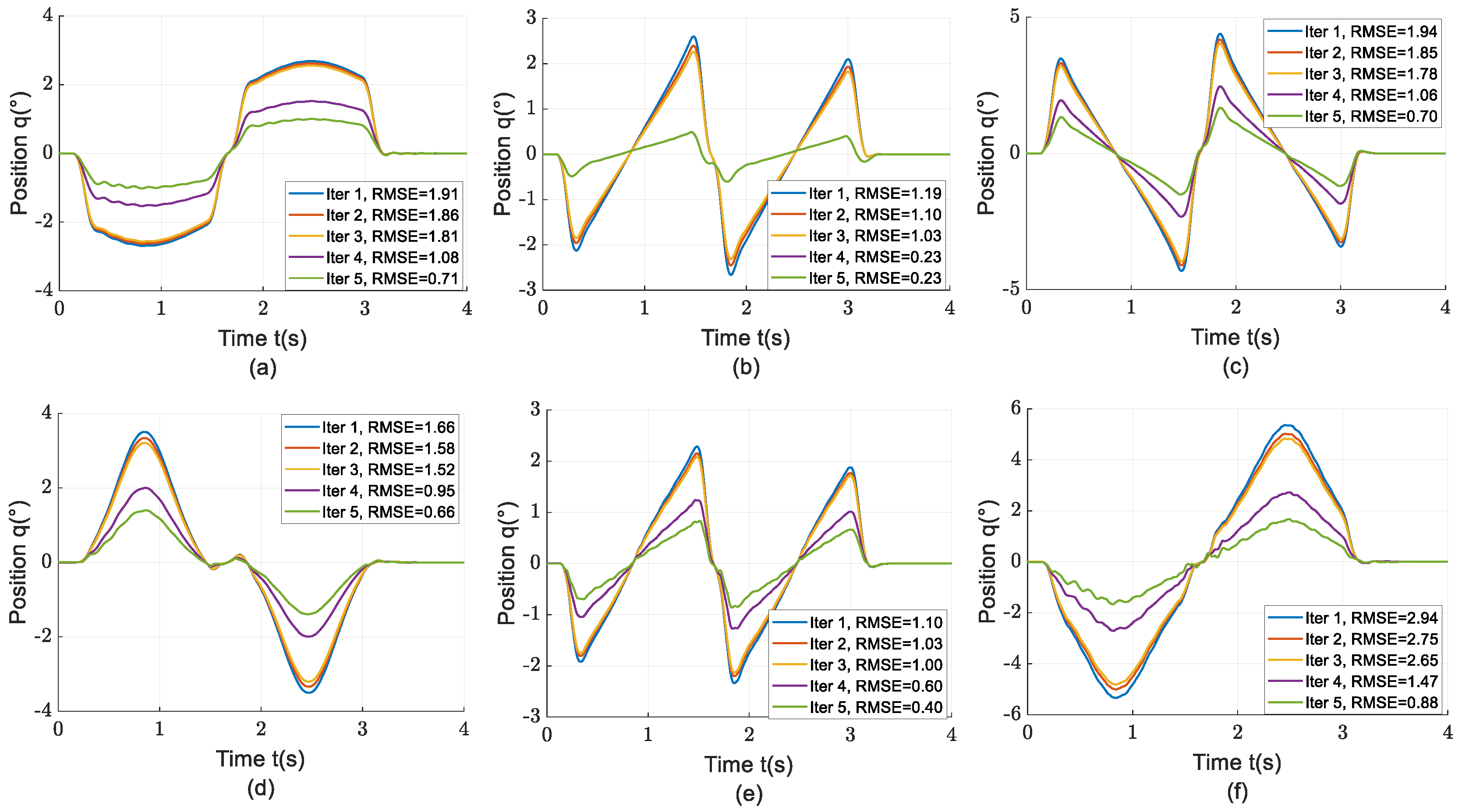
Figure 9.
Joint tracking error curves for circular trajectory. (a) error of joint 1, (b) error of joint 2, (c) error of joint 3, (d) error of joint 4, (e) error of joint 5, (f) error of joint 6.
Figure 9.
Joint tracking error curves for circular trajectory. (a) error of joint 1, (b) error of joint 2, (c) error of joint 3, (d) error of joint 4, (e) error of joint 5, (f) error of joint 6.
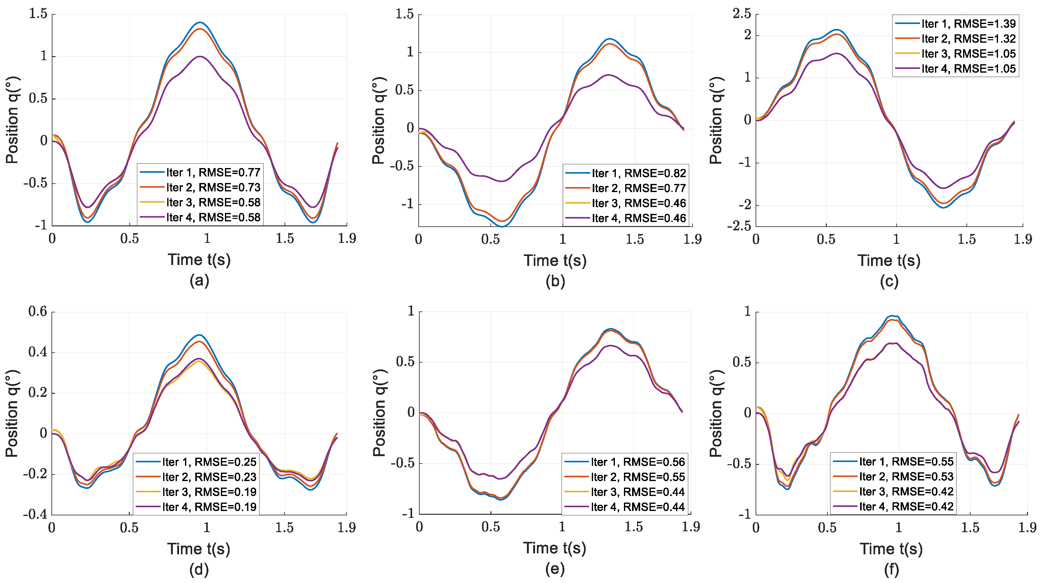
Figure 10.
Cartesian space trajectory curve. (a) XY-plane projection of the linear trajectory, (b) XY-plane projection of the circle trajectory.
Figure 10.
Cartesian space trajectory curve. (a) XY-plane projection of the linear trajectory, (b) XY-plane projection of the circle trajectory.
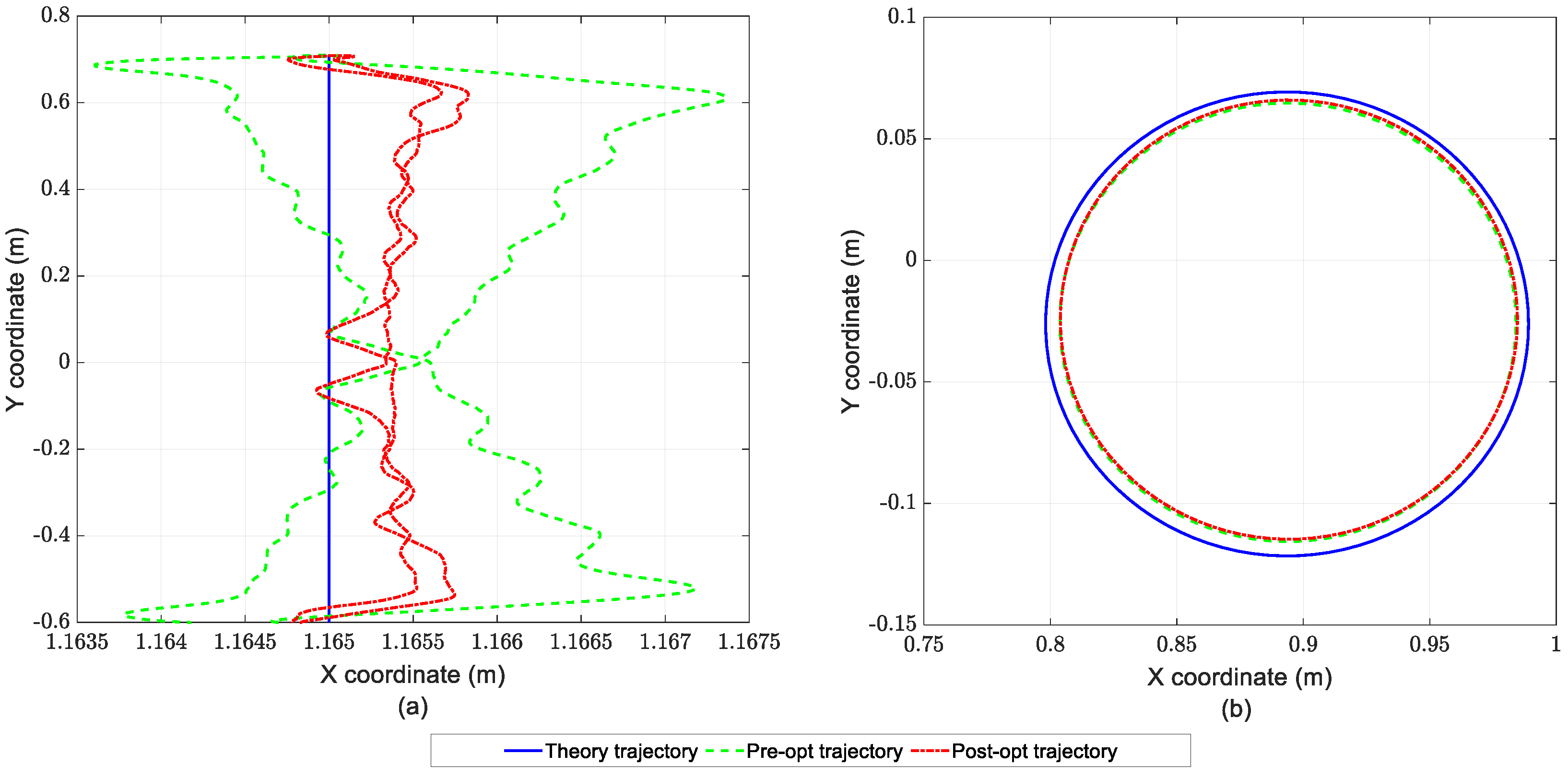

Table 1.
Hyper-parameters of Model Training.
| Hyper-parameters | Value |
|---|---|
| Min_child_weight | 1 |
| Max_depth | 6 |
| Subsample | 1 |
| Colsample | 1 |
| K | 750 |
| 0.1 | |
| 1 |
Table 2.
Comparison of Joint Torque Residuals.
| Type | Index | Joint 1 | Joint 2 | Joint 3 | Joint 4 | Joint 5 | Joint 6 |
| Mechanism Model | RMSE(R1) | 46.407 | 34.774 | 27.583 | 8.689 | 8.133 | 3.059 |
| Hybrid Model | RMSE(R2) | 8.693 | 5.205 | 6.180 | 1.291 | 0.499 | 0.430 |
| Improvement Effect | (R2-R1)/R1 | 81.268% | 85.032% | 77.595% | 85.142% | 93.865% | 85.943% |
Table 3.
Joint Errors Before and After Optimization.
| Type | Index | Joint 1 | Joint 2 | Joint 3 | Joint 4 | Joint 5 | Joint 6 |
| Linear Trajectory |
Pre-optimization RMSE(R1) | 1.91 | 1.19 | 1.94 | 1.66 | 1.10 | 2.94 |
| Post-optimization RMSE(R2) | 0.71 | 0.23 | 0.70 | 0.66 | 0.40 | 0.88 | |
| Improvement Effect | 62.83% | 80.67% | 63.92% | 60.24% | 63.64% | 70.07% | |
| Circular Trajectory |
Pre-optimization RMSE(R3) | 0.77 | 0.82 | 1.39 | 0.25 | 0.56 | 0.55 |
| Post-optimization RMSE(R4) | 0.58 | 0.46 | 1.05 | 0.19 | 0.44 | 0.42 | |
| Improvement Effect | 24.68% | 43.90% | 24.46% | 24.00% | 21.43% | 23.64% |
Table 4.
Trajectory Accuracy Comparison.
| Type | Index | Pre-opt | Post-opt |
| Linear Trajectory |
Average Error | 1.19 | 0.33 |
| Maximum Error | 2.36 | 0.83 | |
| Circular Trajectory |
Average Error | 5.82 | 5.60 |
| Maximum Error | 6.88 | 5.95 |
Disclaimer/Publisher’s Note: The statements, opinions and data contained in all publications are solely those of the individual author(s) and contributor(s) and not of MDPI and/or the editor(s). MDPI and/or the editor(s) disclaim responsibility for any injury to people or property resulting from any ideas, methods, instructions or products referred to in the content. |
© 2025 by the authors. Licensee MDPI, Basel, Switzerland. This article is an open access article distributed under the terms and conditions of the Creative Commons Attribution (CC BY) license (http://creativecommons.org/licenses/by/4.0/).
Copyright: This open access article is published under a Creative Commons CC BY 4.0 license, which permit the free download, distribution, and reuse, provided that the author and preprint are cited in any reuse.


