
Submitted:
25 November 2025
Posted:
26 November 2025
You are already at the latest version
Abstract
New Zealand, located along the boundary between the Pacific and Australian plates, is among the most seismically active regions in the world. In such an area, reliable short-term forecasting of strong aftershocks is essential for seismic risk mitigation. In this study, we apply NESTORE (NExt STRong Related Earthquake), a machine learning probabilistic forecasting algorithm, to the New Zealand earthquake catalogue to evaluate the probability that a mainshock of magnitude Mm will be followed by an event of magnitude ≥ Mm –1 within a defined space–time window. NESTORE uses nine features describing early post-mainshock seismicity and outputs the probability that a cluster is Type A (i.e., containing a strong aftershock) or not (Type B). We assess performance using two testing strategies: chronological training–testing splits and k-fold cross-validation, and refine the training set using the REPENESE outlier-detection procedure. The k-fold approach proves more robust than the chronological one, despite changes in catalogue characteristics over time. Eighteen hours after the mainshock, NESTORE correctly classified 88% of clusters (77% for Type A and 92% for Type B). Notably, the highly destructive 2010–2011 Canterbury–Christchurch sequence was correctly identified as Type A. These findings support the applicability of NESTORE for short-term aftershock forecasting in New Zealand.
Keywords:
machine learning algorithm
; NESTORE
; k-fold validation
; outlier detection
; aftershocks
; New Zealand seismicity
; seismicity clusters
; forecasting
1. Introduction
Aftershocks following large earthquakes can substantially amplify the overall impact of the mainshock by imposing additional loads on already damaged structures, potentially leading to further degradation or collapse, and by disrupting rescue and recovery operations. Large mainshocks are commonly followed by multiple aftershocks with magnitudes ≥ 5. Consequently, reliable estimates of aftershock occurrence probabilities are a critical component of post-seismic decision-support systems for emergency response and early recovery planning.
New Zealand lies along the boundary between the Pacific and Australian tectonic plates, making it one of the most seismically active regions in the world. Several highly destructive earthquakes have occurred during the past century. Among the most devastating were the 1931 Mw 7.8 Hawke’s Bay earthquake, which struck the North Island near Napier and Hastings and caused 256 fatalities [1,2,3], and the Canterbury–Christchurch earthquake sequence, which resulted in 185 deaths and widespread destruction in Christchurch [3,4]. The Canterbury–Christchurch sequence provides a well-documented example of why forecasting strong subsequent events is a crucial issue for seismic risk mitigation: the September 2010 Mw 7.1 Darfield (Canterbury) earthquake was followed by the February 2011 Mw 6.1 Christchurch earthquake [5]. Although the latter event was of lower magnitude, it produced far more severe impacts due to its proximity to the city and the vulnerability of buildings and infrastructure already weakened by the preceding mainshock.
One of the earliest systematic investigations into the expected magnitude of the largest aftershock was conducted by Båth [6]. By analyzing the magnitude difference Δm between a mainshock and its largest aftershock, Båth showed that the mean Δm is approximately 1.2, leading to the formulation of the well-known Båth’s law: the magnitude difference between a mainshock and its strongest aftershock is, to first approximation, independent of the mainshock magnitude. However, the variability of Δm is substantial, and subsequent studies have highlighted that more accurate estimates require consideration of additional sequence-specific parameters (e.g., [7]).
Following a damaging earthquake, both the public and emergency managers are primarily concerned with the probability of further significant seismic activity. For instance, in California the likelihood that a moderate earthquake will be followed within five days and 10 km by a larger event is approximately 5% [8,9]. Operational Earthquake Forecasting (OEF) [10,11] aims to quantify these probabilities using statistical models grounded in empirical observations, including ETAS [12,13] and STEP [14,15].
Many OEF models incorporate three fundamental properties of aftershock sequences: (a) the modified Omori law which governs the temporal decay of aftershock rates [16]; (b) the Utsu relation, which links aftershock productivity to mainshock magnitude [17]; and (c) the Gutenberg–Richter frequency–magnitude distribution [18]. Reasenberg and Jones [19] combined these relations into a time- and magnitude-dependent rate model parameterized by a, b, c, and p, which describe productivity, magnitude scaling, and temporal decay. Region-specific parameterizations have since been developed (e.g., [20]), although the Reasenberg–Jones formulation does not include explicit spatial forecasting. The Short-term Aftershock Probability (STEP) model [14] extends the Reasenberg–Jones approach by incorporating a spatial decay term proportional to r-² and by translating expected aftershock rates into short-term seismic hazard estimates. STEP also accounts for cascading triggering from larger aftershocks and multiple mainshocks. The Epidemic-Type Aftershock Sequence (ETAS) model [12] is the most widely used statistical framework for short-term seismicity. ETAS explicitly models secondary triggering, estimated to account for about 50% of aftershocks [21], and allows model parameters to be updated as an aftershock sequence evolves. When combined with long-term fault-based hazard models, ETAS yields hybrid systems such as the Third Uniform California Earthquake Rupture Forecast (UCERF3-ETAS) model [22], which has been implemented operationally following major earthquakes in California, including the 2019 Ridgecrest sequence [23,24].
In New Zealand, significant effort has been dedicated to developing both short- and medium-term forecasting methods [25]. Notable contributions include the STEP model [14] and the Every Earthquake a Precursor According to Scale (EEPAS) model [26]. Forecasting capabilities also include an ETAS module within the EEPAS system, the national ETAS-Harte implementation [27], and more recent hybrid approaches such as the Hybrid Forecast Tool (HFT) [28].
An alternative to statistical seismicity-rate models is the use of pattern-recognition approaches for forecasting strong aftershocks. These methods evaluate one or more features of early aftershock activity to determine whether their values indicate that a large subsequent event is likely. Typically, a threshold on Δm is defined, and the predictive capability of selected features is assessed with respect to whether the largest aftershock will have a magnitude deficit smaller than this threshold.
Early pattern-recognition studies by Vorobieva and Panza [29] and Vorobieva [30] introduced a set of diagnostic functions designed to identify premonitory phenomena associated with Δm ≤ 1. Within these frameworks, the strongest forthcoming aftershock is treated as a critical point (a singularity), and—consistent with nonlinear dynamical systems theory—the approach to this critical state is expected to manifest as marked variations in observable seismic parameters, such as elevated activity rates or increased irregularity. Physically, these changes can be interpreted as an enhanced sensitivity of the lithosphere to tectonic loading during the preparatory phase of a strong aftershock. Gentili and Bressan [31] identified a relationship between Δm and the radiated energy of early aftershocks using a dataset of sequences from northeastern Italy (1977–2007). This work was expanded in Bressan et al [32], which further explored connections among Δm, stress drop, and released energy. Other studies have focused on the parameters a and b of the Gutenberg–Richter relation. Shcherbakov and Turcotte [33] proposed a modified form of Båth’s law based on extrapolating the Gutenberg–Richter distribution, in which the magnitude of the largest aftershock is estimated from the ratio a/b. Chan and Wu [7] applied approaches based on both b alone and a–b jointly to four Taiwanese sequences, finding that the performance of each method varied across sequences. Gulia and Wiemer [15] developed a forecasting method based on b-value variations aimed at identifying cases where Δm ≤ 0. However, this approach is limited by the high instability of b estimates when only a small number of aftershocks are available. To address this issue, Gulia et al. [34] proposed an enhanced method using the b-positive formulation [35] to distinguish between a typical decaying aftershock sequence—characterized by b > 1—and sequences likely to culminate in a strong aftershock, which exhibit negative b-values.
In this study, we apply the NESTORE (NExt STrOng Related Earthquake) algorithm—a data-driven, supervised-learning approach for identifying seismic clusters likely to generate strong aftershocks—to New Zealand seismicity. As in Vorobieva and Panza [29] and Vorobieva [30], we adopt a threshold of Δm = 1 to distinguish cluster types: clusters with Δm ≤ 1 are classified as Type A, while those with Δm > 1 are classified as Type B. The algorithm has previously been deployed successfully in several regions worldwide, including California, Italy, western Slovenia, Greece, and Japan [36,37,38,39,40,41,42,43,44]. Over time, NESTORE has been progressively refined to enhance robustness and adaptability across different seismic environments. In this work, we introduce further improvements to the performance-evaluation framework.
The paper is structured as follows. Section 2 provides an overview of the seismotectonic setting of New Zealand and the catalogue used. Section 3 describes the NESTORE methodology, highlighting the modifications introduced in this study. Section 4 presents the results obtained using two distinct testing strategies. Finally, Section 5 discusses and interprets the differences between these results, compares them with outcomes from previous regional applications, and explores possible physical explanations for some of the observed behaviors.
2. Analyzed Region
2.1. Seismotectonic
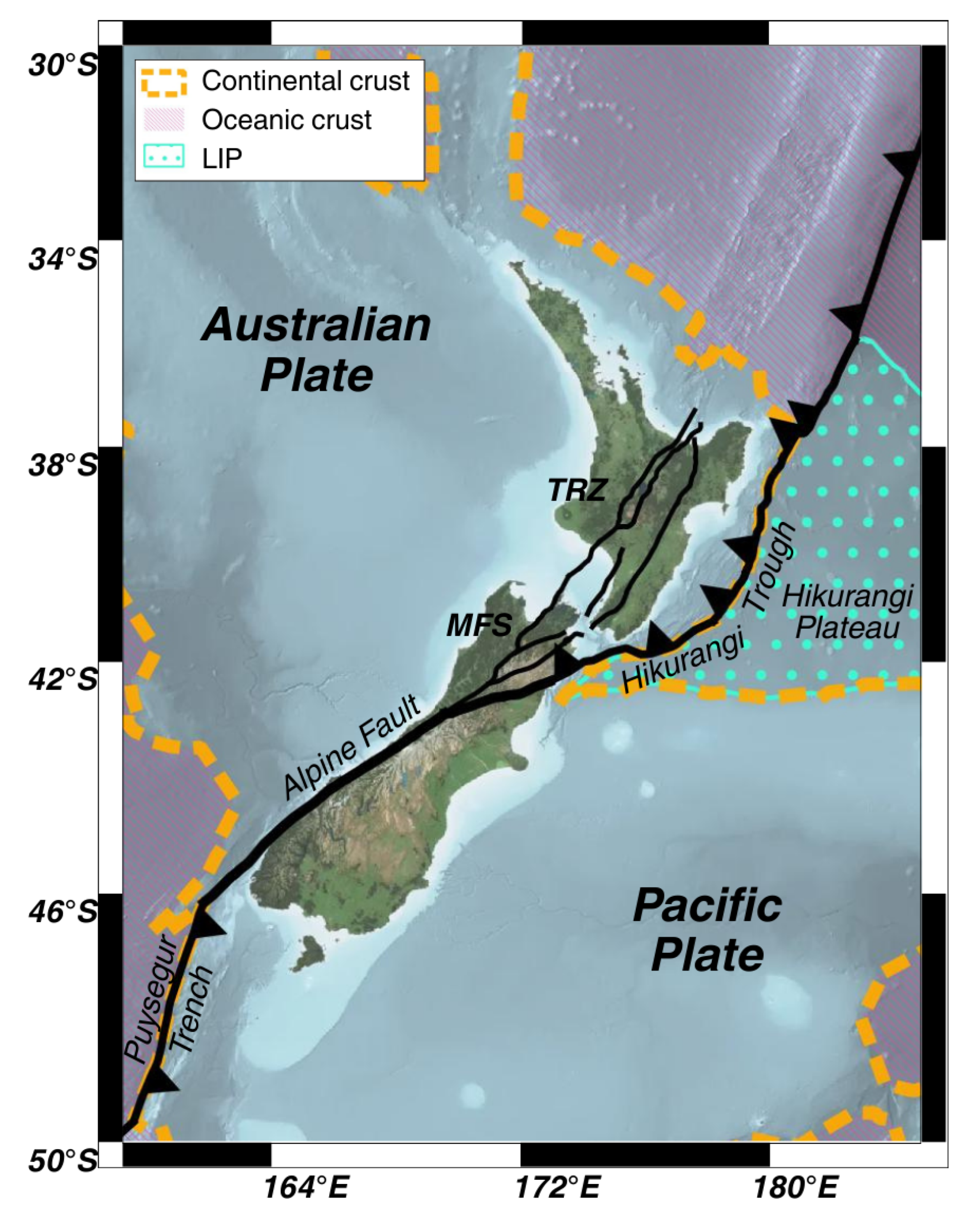
New Zealand is a residual, surficial portion of Zealandia [45], a continent formed in the Mesozoic along the subduction margin of Gondwana [46], which is now crossed by the Pacific-Australian plate boundary (Figure 1). This complex plate boundary system interests the whole country, except for the far north of the North Island and the far southeast of the South Island and has generated 28 earthquakes of magnitude equal or above 7 since 1900 [47]. The general relative motion of the Pacific plate to the Australian plate ranges between 32–49 mm/yr [48], changes from north to south and generates frequent earthquakes with depths ranging between 0 and 600km [49].
One of the two existing subduction interfaces between these tectonic plates is the west-dipping Hikurangi subduction zone, located off the East Coast of the Northern Island, where the Hikurangi Plateau, an Early Cretaceous, intra-oceanic Large Igneous Province (LIP), subducts beneath the Australian plate. Along the interface, the Pacific slab generates earthquakes up to 300 km [50] but extends up to 900km of depth [51]. The back-arc rifting deformation related to this margin is the Taupō Rift Zone (TRZ), a forearc opening basin, that in the Northern Island led to the formation since Quaternary of the active Taupō Volcanic Zone [52].
This boundary segment is followed in the northern part of the South Island by the intra-continental Marlborough transfer zone, a plate corner hosting the subparallel strike-slip Marlborough Fault System (MFS), which in November 2016 was capable of generating a Mw 7.8 earthquake in Kaikōura. This transfer zone accommodates subduction to the strike-slip Alpine fault, a 460 km-long southeast-dipping continental transform located in the South Island that formed in the Late Oligocene; along with the Hikurangi Thrust, the Alpine Fault accommodate for the 80% of the relative plate motion occurred during the Quaternary [53] and according to Sutherland et al. [54], it is realistic to expect Mw≥8 earthquakes. Looking at a closer scale, the Alpine Fault consists of both thrust and strike-slip segments [51], of which the latter are parallel to the plate motion vector of the two tectonic plates [55].
Offshore the South Island, the Alpine Fault becomes vertical and is followed by the 400km long, southeast-dipping Puysegur subduction zone. Here, the subduction phase of the Australian plate beneath the Pacific place is still at an early stage, begun in Miocene–Quaternary [56], and generated only one Quaternary volcano (Solander Island) [57]. The earthquakes hypocenters can reach up to 150km of depth [58].
Figure 1.
Present-day tectonic setting of New Zealand Aotearoa along the obliquely convergent Pacific–Australian plate boundary. LIP: Large Igneous Province; TRZ: Taupō Rift Zone; MFS: Marlborough Fault System. Map created using geospatial layers from the TRAMZ data © GNS Science 2020 [59]. Additional data sources listed in the Data Availability section.
2.2. Catalog
In the 1970s, the seismic network in New Zealand already comprised 26 stations [49]. The first broadband digital seismic stations were installed in the late 1990s, preceding the start of the GeoNet initiative in 2001 [60]. This program provides for the production and maintenance of New Zealand’s national operational catalog (Earthquake Information Database, EID), which currently operates 120 short-period and 65 permanent broadband stations. Along with network improvements, different location methods and magnitude scales have been proposed over time (for more details, see [49]).
To analyze New Zealand seismicity, we used two seismic catalogues (see Data Availability section for further details):
We focused on shallow earthquakes with a maximum hypocentral depth of 50 km, due to possible viscoelastic effects: deeper events may result in different seismicity characteristics for clusters (see, e.g., [40,41,43]). Our analysis began in 1988 to avoid gaps in the magnitude range recording that we detected, which are probably related to the merging of different catalogues. In addition, we selected clusters whose mainshocks are onshore, to avoid errors in location and magnitude related to inaccuracies in event location and (consequently) in magnitude assessment. The analysis area we selected is highlighted in red in Figure 2.
Regarding the magnitude scale adopted, both catalogues report earthquake magnitudes in various units. The magnitude (Mstd) proposed as preferred by Christophersen et al. [49] approximates Mw but is not yet available in GeoNet Quake Search for recent events. Since NESTORE has mainly been applied to local magnitudes, and to maintain consistency within the dataset, we used ML.
The New Zealand Earthquake Catalogue lists ML magnitude for almost all events; starting with 1988 the value of ML is missing in a very small percentage of cases (0.002%), mainly corresponding to offshore events. For the GeoNet Quake Search system, we derived ML where missing using orthogonal regressions on other magnitude scales. In order to have a large and revised dataset for the regression we used New Zealand Earthquake Catalogue data. Figure 3 shows the data we used and their fitting line; Table 1 shows the corresponding regression coefficients. Overall, the data of the GeoNet Quake Search system we used from 2020 to 2025 comprised approximately 66,000 earthquakes, with ML available in 96% of cases. When ML was not available, we used the preferred magnitude suggested by the catalogue. For about 1,000 events, the preferred magnitude was MLv, the local magnitude estimated from the vertical component of the signal instead of the horizontal components. For approximately 1,800 events, the preferred magnitude was what the catalogue lists as “M”, which is a combination of MLv, moment magnitude Mw(MB) estimated from body wave magnitude, and the number of stations supplying Mw(MB) (see https://www.geonet.org.nz/data/supplementary/earthquake_location for further details). Only in two cases the preferred magnitude in the GeoNet Quake Search system was Mw(MB), and in one case it was Mw. However, these three events are offshore, far from the coast, and are not considered in our cluster analysis.
To obtain reliable results that are not affected by artefacts from the network’s inability to detect smaller events, it is necessary to use data above the completeness magnitude, which is the magnitude above which all earthquakes are detected. Figure 4 shows how completeness magnitude varies spatially. The completeness magnitude was estimated using the maximum curvature method [64] plus 0.2 to account for the method’s tendency to underestimate completeness magnitude (e.g. [43]). The analysis was performed by Zmap software [65] on declustered catalogue (see the next section for applied declustering method). Within the region highlighted in Figure 2 by the dotted red line, the completeness magnitude Mc is generally ≤ 3; the two exceptions are due to border effects: in the south, because the cell contains offshore events, in the north, because seismicity is low and the algorithm automatically extends the search area to offshore events. We therefore selected Mc = 3 as the minimum magnitude for our analysis across the entire area. Within this area, only one event was missing ML in the New Zealand Earthquake Catalogue: an earthquake with Mw=7.8 on 15 July 2009 in the southwestern part of the analyzed area, which had a too close in time strongest aftershock (~20 minutes) to be analyzed by NESTORE (NESTORE performs the first analysis 6 hours after the mainshock to ensure reliable statistical information).
3. Methods
NESTORE is a supervised machine learning based algorithm that aims to forecast the class of clusters of seismicity defined by the difference in magnitude between the mainshock and the strongest aftershock: if this difference is equal to or less than 1, i.e. Mm - Maf t≤ 1, the cluster is defined as “Type A”, otherwise as “Type B”.
NESTORE algorithm evolved during time. NESTOREv1.0, the Matlab code available on GitHub (see Data Availability section) was described in Gentili et al. [39]. The code is divided into four modules that can be executed independently of each other: Cluster identification module, Training module, Testing module, Near-Real-Time module. In this paper, we describe the first three modules that were used in this work (3.1, 3.2, 3.4). Gentili et al. [43] proposed a further algorithm, named REPENESE, added to the training module to remove the outliers from the training set and obtain more stable results (see Section 3.3). The last subsection (3.5) describes the last innovations we introduced in this paper for a more robust estimate of the performance.
3.1. Cluster Identification
Cluster identification is the first module of NESTORE, in which the seismic clusters are selected and stored to be available for the following steps. Choosing the best method for this task is not trivial, especially when the clusters are close to each other both in time and space, which is very often the case for earthquakes. One of the simplest yet widely used methods, which has been successfully applied in most of the previous works on NESTORE [36,37,38,40,41], is the so-called window-based method. In this approach, earthquakes belonging to clusters are selected within circular areas centered on the largest events. The radius of each circle depends on the magnitude Mm of the corresponding large event. Similarly, the temporal extent of the cluster depends on the magnitude Mm of the corresponding large event. If one of these events is already within the spatiotemporal domain of a previous event, the clusters are merged. Several authors have proposed laws for evaluating region-specific radius and time window length (e.g. [31,66,67,68,69,70]). For our application in New Zealand, we have found that the law for the radius proposed by Christophersen [71], which has a dependence on magnitude similar to that proposed by Utsu and Seki [72] and Kagan [68], best define the clusters; similarly, the best time extent is obtained with the Gardner and Knopoff law [66]. Following the approach of Anyfadi et al. [40], we selected these laws by comparing the duration and extent of manually estimated clusters with functions proposed in literature. The equations we adopted are therefore the following:
where Mm is the magnitude of the strong event generating the cluster, r is the radius of the cluster and t is its duration.
To ensure the functionality of NESTORE, the completeness magnitude within each cluster must be greater than Mm - 2. Having selected a completeness magnitude of 3 for the entire region, we have chosen 5 as the magnitude threshold for Mm. Note that, since our method is developed to work in semi-real time, the strong earthquake generating the cluster may not always be the mainshock, but it may be a strong foreshock of a stronger following mainshock. To avoid confusion, in NESTORE the strong event is called “operative mainshock” (o-mainshock for simplicity).
3.2. Training
In the training module, an input dataset with known classes of seismic clusters is used to train the classifier. Unlike versions of NESTORE prior to 2025, the dataset selected for training is preliminarily filtered to remove outliers using the REPENESE algorithm (see Section 3.3). The Training module is divided into four sub-blocks.
3.2.1. Feature Extraction
Nine seismic features are calculated within each cluster of seismicity, based on the cumulative source area, the energy released, the magnitude, the number and spatial distribution of events (see Table 2). The features are computed at increasing time intervals Ti starting from one minute after the mainshock (for an analysis of the reason of this interval see [38]) up to 0.25, 0.50, 0.75, 1, 2, 3, 4, 5, and 7 days after. For simplicity, we will refer to Ti = x hours as the interval ending x hours after the mainshock.
Note that we analyze Type A clusters until the first strong aftershock with M ≥ Mm -1 occurs, because after that the class is already defined (so further testing is not useful), and the subsequent seismicity results from the complex superposition of the aftershocks from both the mainshock and the strongest aftershock, potentially causing anomalous behavior. Therefore, the cardinality of class A changes depending on the interval Ti and decreases over longer intervals.
3.2.2. One-Node Decision Tree
Once the features are extracted, a decision tree is trained for each feature at every time interval to discriminate between the A and B class clusters. Small databases, such as in our case, are likely to experience overfitting; therefore, the number of parameters should be kept small. NESTORE uses a one-node tree so that a feature is considered successful in class discrimination if most Type A cluster feature values are greater than the threshold and most of Type B are lower. If no suitable value can be found, the threshold is set to NaN and the corresponding feature for that time interval is discarded.
3.2.3. Selection of Good Interval
The threshold performances (and the corresponding time intervals) are evaluated using the Leave-One-Out (LOO) method. This special case of k-fold cross-validation is suitable for small datasets, as each sample is tested with a classifier trained on all the other samples in the dataset. The reliability of the classifiers is then expressed in terms of Accuracy, Precision, Recall, and Informedness. The first three parameters range from 0 to 1, and the last one from -1 to 1. A feature calculated over a given time interval Ti is considered relevant for classification if: (1) Accuracy, Precision, and Recall are greater than 0.5; (2) Accuracy is greater than or equal to the accuracy achieved by always predicting the most frequent class; (3) Informedness is greater than 0. The class distribution in our case study is consistent with previous applications of NESTORE: class B clusters are more frequent than class A [36,37,40,41,43,44], and therefore the second condition is crucial to account for class imbalance. The interval in which the feature can be used (the “good interval”) begins at Ti = s1, the first interval where the feature is considered relevant, and ends at Ti = s2, where s2 is the time interval with the highest Informedness. The performances are illustrated using Precision-Recall and Receiver Operating Characteristic (ROC) diagrams.
3.2.4. Inheritance, Validation and Probability Estimation
For time intervals larger than s2, the feature is not removed from the classification, but both the feature values and the corresponding thresholds are inherited from the s2 time interval. To verify that the inheritance process does not add errors to the classification, the LOO method is applied once more for time intervals larger than s2 to compute the percentage of Type A correctly classified (hit rate) and the percentage of misclassified Type B (false alarm rate). The intervals Ti in which hit rate < false alarm rate are discarded, the corresponding thresholds are set to NaN, and the feature is not considered for the classification. The training ends when the time intervals of usability are validated. Then, for each feature and time interval, the probability of being a Type A cluster above and below the threshold is estimated. The training output consists of four vectors: (1) the thresholds vector for each good interval; (2) the validity vector, providing the time ranges of validity for each feature; (3) the probability vector, which gives, for each feature of every seismic cluster, the probability of being Type A above and below the threshold; (4) the NAB vector, i.e. the number of class A and class B clusters for each Ti.
3.3. REPENESE
As previously mentioned, our dataset is limited in the number of samples and imbalanced in class distribution, as Type B clusters occur much more frequently than Type A clusters. The same issue was identified in earlier applications of NESTORE, prompting Gentili et al. [43] to develop a specific algorithm for outlier detection. The goal is to better refine the training dataset to ensure more reliable thresholds and a clearer distinction between the classes. The algorithm was developed based on the following considerations for outlier selection: (1) it uses only relevant features; (2) it accounts for the class imbalance; (3) it replaces the commonly used concept of “cluster centroid distance” in outlier detection algorithms with a simpler and more appropriate distinction between “under” and “above” the threshold. In this way, features with values far from the centroid, but correctly assigned, are still considered. The resulting algorithm was named REPENESE and proceeds through the following steps:
- RE: Relevant Features. Features are relevant if there exists a threshold for which (1) the true-positive rate is greater than 0.5, (2) the false-positive rate is less than 0.5, and (3) Precision is greater than 0.5.
- PE: class imbalance PErcentage. The probabilities of being Type A (PA) or Type B (PB) for a cluster are calculated from the percentages of Type A and Type B samples in the training set, thus providing an assessment of the asymmetry between the classes.
- NE: NEighborhood detection. For each relevant feature, the values are sorted. To determine whether a value is an outlier, its neighborhood is defined by considering the closest N1 larger and smaller values for the Type A and Type B class, respectively. The dimension of the neighborhood, Sn, is the total number of observations within it, while N is the number of samples of the class considered.
- SE: SElection. The sample is a possible outlier if N≤P⋅Sn, with P being PA or PB depending on the sample class. Samples are considered to be true outliers if they are consistently outliers across all relevant features and time periods for which they are analyzed.
For this work REPENESE has been automatized through the implementation of an independent module.
3.4. Testing
The aim of the testing module is to forecast the class of clusters from an independent test set by using the information gained in the training phase. The new catalog undergoes a similar procedure to the one described so far. After the cluster identification phase, the features for each cluster are extracted at each time step Ti specified in the Validity vector. The Threshold vector obtained after the outlier removal made by REPENESE is compared with the calculated features. In accordance with the existing thresholds, the Probability vector (referred instead to the whole training dataset, outliers included) is used to evaluate the probability that the cluster class is A if the nth feature is present at time Ti:
Gentili and Di Giovambattista [37] have proposed an approach based on Bayes’ Theorem to combine the feature-based probabilities and estimate for each given cluster the probability at each time Ti that it is of Type A:
N(A)i and N(B)i are retrieved from the NAB vector. By including the cardinality of each class in the data set, the imbalance between the classes is taken into account. For the final evaluation of the quality of the algorithm result, the actual known class of the clusters is compared with the classification output. The ROC and Precision-Recall diagrams are re-generated to better visualize the performance of the algorithm.
3.5. NESTORE Performances Validation
In previous versions of NESTORE, the dataset was divided into two distinct subsets –a training set and a test set– to enable independent evaluation of model performance. The division was based on the year of occurrence of each cluster’s mainshock. This setup allowed for a retrospective forecasting procedure: the model was tested as if performing a real-time forecast of the cluster class, and, since the actual class was known afterwards, its predictive performance could be quantitatively assessed.
In this study, we adopt an additional evaluation strategy. Rather than assigning only the most recent data to the test set, we use a stratified k-fold cross-validation approach [73]. In k-fold cross-validation, the dataset instances (in this case, the clusters) are randomly divided into k groups, or folds, of approximately equal size. Each fold is used once as a validation set, while the remaining k-1 folds are used for training. The overall performance of the method is then calculated as the mean performance across all k validation folds.
Compared to a simple train–test split, this approach provides a more reliable performance estimate, as it uses all available clusters for both training and validation, and avoids overfitting, since the training and test sets are disjoint for each iteration. The leave-one-out (LOO) method discussed in Section 3.2.3 is a special case of k-fold cross-validation where k equals the total number of instances in the dataset.
The stratified variant of k-fold cross-validation further improves the scheme of the k-fold cross validation by preserving the original class distribution within each fold. This is particularly advantageous for classification problems involving imbalanced datasets, as it reduces the risk of biased performance estimates due to underrepresented classes.
Overall, this cross-validation approach yields a more robust and comprehensive assessment of model performance than a simple time-based data split, as it leverages the entire dataset—provided that the time of cluster occurrence does not affect the data quality.
A further analysis has been introduced in this latest version of NESTORE (see also Gentili et al., 2025b 44), namely the probability α of obtaining h or more hits (Type A clusters correctly classified) by chance. This probability was calculated according to Zechar [74] as:
where τ represents the fraction of the “space” occupied by alarms within the testing region. Here, “space” should not be interpreted in a purely geometrical sense (e.g., in kilometers or degrees). In the analyses conducted within the framework of the Collaboratory for the Study of Earthquake Predictability (CSEP) testing centers [75,76], the “space” coincides with the testing region that is defined as the Cartesian product of the binned magnitude range of interest and the binned spatial domain of interest.
In this study, τ is defined as the ratio between the number of clusters classified as Type A and the total number of clusters. Although in some applications related to mainshock forecasting the measure of time-space may not be uniquely defined [74], in this context τ is uniquely determined, thus avoiding ambiguous results. In this formulation, N denotes the number of observed Type A clusters. A smaller value of α corresponds to an alarm with higher skill.
4. Results
To analyze NESTORE on New Zealand seismicity, we adopted three approaches:
- “Chronological”, i.e. time-based analysis: training was performed using clusters from1988 to 2013, and testing using clusters from 2014 to 2025.
- “K-fold”, i.e. based on stratified k-fold analysis. We used k=3.
- “Autotest”, i.e. an analysis in which the same dataset is used for training and testing coincide.
Regarding the Chronological and k-fold methods, free parameters (the starting year of testing and the number of folds k) were chosen to maximize the reliability of results. For small datasets, the quality of performance evaluation improves as the number of available instances of the two classes in the test set increases, because the data distribution is more accurately represented. However, for the same reason, the classifier’s performance also improves as the number of instances of the two classes in the training set increases. Since the number of instances is low and the training and test sets are disjointed, there is a trade-off between the size of the training and test sets. NESTORE performs testing if at least three instances of the class with lower cardinality are available. With a total of 14 Type A clusters, we selected a 3-fold stratified analysis. In this way, each fold contains four or five Type A instances. Similarly, in the chronological approach, we chose the testing starting year to ensure four Type A instances.
The autotest was not considered for assessing classification performances, as using the same set for training and testing may lead to overfitting and thus provide an “optimistic” estimate of the algorithm’s performance. The outlier filtering performed by REPENESE partially mitigates this effect, because outliers do not contribute to threshold evaluation in training, while they are in the test-set. The autotest testing should be regarded as an analysis of the dataset’s internal consistency, because if it fails to predict a cluster class, this indicates that this cluster is an outlier whose behavior is so anomalous compared to the other clusters of its class in the training set that it cannot be assimilated to the others, even by an ad hoc choice of features.
Table 3 shows the number of training and testing instances in the different approaches. The dataset appears unbalanced, as the cardinality of class B is approximately three times that of class A.
Figure 5 shows the map of the epicenters of o-mainshocks of the clusters (red for Type A clusters, blue for Type B clusters). Crosses indicate the clusters that are misclassified in all time periods of the analysis. While the chronological analysis does not reveal any misclassification, the k-fold analysis shows five clusters misclassified in all time intervals, of which three are Type A and two are Type B. It is interesting to compare this result with that of the autotest. In this case, four clusters remain misclassified, highlighting how different they are from the corresponding Type A and Type B populations, such that NESTORE cannot classify them in the corresponding class, even when specifically trained on it. Three of these four clusters were detected as outliers by REPENESE and not used in the following training. The two 2005 clusters misclassified by the k-fold approach, with o-mainshocks on January 20 and on June 23, were not recognized as outliers by REPENESE and were included in the training with all available data; the autotest training included the clusters and attempted to adjust the thresholds according to those clusters classifications. The testing shows that the obtained thresholds were able to correctly classify the January cluster but not the June one. This correct result in the January cluster case may be due to overfitting, which tunes the threshold to include that data, or to sparse data near the threshold that do not allow for precise threshold determination in the smaller K-fold training set. In order to understand which of these hypotheses is correct, a large independent dataset will be necessary, analyzing the seismicity in the following years.
The black arrow shows the 2010-2011 Canterbury-Christchurch cluster, that was correctly classified by NESTORE as a Type-A cluster.
Figure 6 shows the performance of the method in the three cases, using the ROC diagram. Binary classifier analyses are based on two classes: the positive and the negative class. In our analysis, we define class A as positive and class B as negative. The ROC graph displays on the horizontal axis the normalized (to 1) percentage of negative class instances wrongly classified (False Positive Rate - FPR); in our case, this corresponds to the normalized percentage of B clusters wrongly classified. The y axis shows the normalized percentage of positive instances correctly classified. This normalized percentage is called True Positive Rate (TPR), or Recall, or hit rate. In our case, this is the normalized percentage of A clusters correctly classified. The random classifier corresponds to the diagonal dashed line. The ideal classifier corresponds to TPR=1 and FPR=0 (upper left corner) and the closer the classifier is to the point (0,1), the higher its performance. Unsurprisingly, the autotest (Figure 6c) supplies better results than the k-fold, with recall in the range [0.64, 0.77] depending on the time period, and a very low value of false positive rate [0.03, 0.08]. The best results were obtained for Ti=18 h or 1 day (superimposed symbols). These results should be considered as an upper limit for correct performance estimation, as they are likely too optimistic due to possible overfitting. However, even with the k-fold analysis (Figure 6b), the performance remains high, well above the dashed line, corresponding to a random response. In this case as well, the best performance was obtained for time interval Ti=0.75 days (18 hours). Specifically, for Ti=18 h or 1 day the recall is 0.77 and the FPR is 0.08.
Note that for long time intervals, greater than or equal to 3 days, the FPR is minimal in the autotest case but not in the k-fold case. We hypothesize that this is due to overfitting. For time periods longer than 3 days, all thresholds are inherited, and differences in performance may be due only to the decrease in Type A clusters in the dataset.
More in detail, comparing Figure 6, Figure 5 and the output classification of individual clusters for Ti=18 hours we can see that K-fold and autotest provide similar results. The recall of 0.77 is identical in both cases and is due to the correct classification of the same 10 out of 13 A clusters. The only difference is that in the autotest case, 2 B clusters were classified as A, while in the k-fold case, 3 were classified as Type A, resulting in FPRs of 0.05 and 0.08 respectively. Comparing this result with Figure 5, the three misclassified Type A clusters are the ones identified as outliers for all time periods (red crosses). Conversely, the B clusters misclassified for Ti=0.75 days are not all shown in Figure 5, because one of the three (with o-mainshock on 26 July 2012, ML=5) was correctly classified at Ti≥3 days.
Figure 6a shows the performance of the chronological analysis. In this case, the performances are better than the others. The chronological approach achieves ideal classifier performance 12 hours (0.5 days) after the o-mainshock and maintains the same classification for all the following time intervals. The reason for such good performance is that the testing phase starts in 2014, while the last outlier cluster in chronological order is in 2010. We will discuss this result in more detail in the discussion and conclusion section.
To validate these analyses, we evaluate the probability α of obtaining h-hits by chance, according to equation 3. Table 4 shows the probability in the three cases for Ti=0.75 days, which is the shortest time interval for which the three approaches provide the best results (as in the previous analysis, autotest results should be considered as a lower limit for alpha). In all cases, this probability is less than 1%, showing the good performance of the method. Note that the chronological approach α has higher values due to the smaller dataset involved.
The Precision-Recall graphs in Figure 7 show Recall on the horizontal axis, which coincides with the true positive rate (FPR) shown in Figure 6, and Precision on the vertical axis; Precision, in our case, is the normalized percentage of clusters classified as A that are indeed A. Precision is a very important evaluation parameter in an unbalanced dataset because, if the negative class is larger than the positive one, even a small percentage of misclassified negative instances may result in a large percentage of events wrongly classified as positive. The random classifier corresponds to the normalized percentage of positives in the dataset. As the percentage of A in our dataset decreases over time, we show the line for the smallest time interval and the largest percentage, as this is the most conservative approach. The ideal performance for the Precision-Recall graph is Precision=Recall=1, so the closer the symbol is to the upper right corner (1,1), the better the classifier. Again, both the autotest and the k-fold confirm that the best performances are obtained for 0.75-1 day time intervals. K-Fold analysis yields a Precision of 0.75 (compared to 0.83 in the autotest case). In terms of Precision, the best performances are obtained in autotest for intervals equal to or longer than 3 days, due to the lower FPR outlined in the ROC graph. These performances are not confirmed by K-Fold analysis, in which, conversely, Precision decreases for larger time intervals. This result is possibly related to overfitting in the autotest approach like in the ROC diagram case. The Accuracy (i.e. the normalized percentage of correctly classified clusters) of the three methods for Ti=18h is: 1 for the Chronological approach, 0.88 for the K-Fold analysis, and 0.90 for the autotest.
Note that, while in the testing analysis autotest results should be regarded as an (optimistic) upper limit on possible performance, in the case of training and threshold determination, the more reliable thresholds are those obtained by the autotest approach, as they use the entire available dataset. These are therefore the thresholds that should be used when applying the method to future clusters of seismicity.
Table 5 shows the obtained thresholds. Values in bold are calculated for the corresponding time interval, while the others are inherited values.
All features except Vm and N2 contribute to the classification at Ti=0.75 days according to the thresholds shown in the table. Vm and N2, which supply the best results 6 hours after the o-mainshock, also contribute to the classification, but by using inherited values.
5. Discussion
This work should be considered in the context of the broad application of the NESTORE method in several countries beyond New Zealand, including Italy, Slovenia, California, Greece, and Japan [36,37,38,40,41,43](Gentili and Di Giovambattista, 2017 36, 2020 37, 2022 38; Anyfadi et al., 2023 40; Brondi et al., 2025 41; Gentili et al., 2025 43). The performance evaluation approach used in this paper, which employed the stratified k-fold method rather than the chronological approach, should be seen as part of the ongoing improvement of NESTORE across successive applications, with the aim of making the algorithm more stable and the performance assessment more accurate.
As in most applications of NESTORE to other regions [36,37,38,40,41,43], the dataset is small and unbalanced, with the cardinality of class B approximately three times that of class A (see Table 3). A review of the results obtained in previous applications of NESTORE is currently under revision [44]. In other applications, NESTORE successfully classified 66–100% of Type A clusters and 90–100% of Type B clusters. The model’s Precision, representing the proportion of correctly identified Type A clusters among all those predicted as Type A, ranged between 0.75 to 1, with lower values observed under strong class imbalance favoring Type B clusters. In the application to New Zealand, for the time interval of 18 hours after the mainshock, if the chronological approach is used, the Precision was 1 for both classes, with 100% of clusters correctly classified. In the K-fold analysis, 77% of Type A and 92% of Type B clusters were correctly classified, and the Precision was 0.75. Therefore, both results are in good agreement with other applications of the method.
To account for the small dataset, we verified the probability α of obtaining the observed h-hits (Type A correctly forecasted) by chance. This probability is less than 1% in both the k-fold and chronological approaches, although it is higher for the chronological approach because the dataset is smaller. This result is consistent with applications to other countries, where α ranges from 0.1% to 4% [44].
An important point to discuss is whether, for future classifications, the more reliable performance estimate for New Zealand is provided by the chronological approach or the k-fold approach. One reason to consider the chronological approach carefully is that, while the k-fold results are worse than the autotest results, the chronological approach yields better results. As the autotest results should be regarded as an upper bound (an optimistic estimate of performance) due to possible overfitting, we expected its performance to be the best. If the quality of the catalogue in terms of location and magnitude assessment, at least for earthquakes with magnitude greater than 3, had remained unchanged over time, the k-fold approach would be the most reliable approach, as it analyses a larger dataset, i.e. the entire available database. However, it is well known that the quality of seismic catalogues generally changes over time, due to the increased number of stations, higher quality sensors, improved location algorithms, et cetera. As mentioned in Section 2.2, in New Zealand the seismic network and the data processing evolved with time [49]. A major change since the beginning of the instrumental era has been the switching to the open-source earthquake analysis program SeisComP (SC) [77] in 2012. Notably, all outliers occurred before 2012. We therefore test the null hypothesis H0 that this timing of outliers is due to chance, against the alternative hypothesis H1, that the absence of outliers is not random (possibly related to independent causes, such as catalogue quality). We hypothesize that the occurrence of outliers follows a Poisson distribution and estimate the probability of observing no outliers. From 1988 to the end of 2011, there are 24 years in which we detected 5 outliers according to k-fold, while from 2012 to 15 May 2025, we have 13.37 years with no outlier. The annual mean of outliers in the catalogue is therefore 0.21 outliers per year, corresponding to μ = 2.78 outliers in 13.39 years. According to the Poisson distribution, the probability of having x = 0 outliers is therefore:
In this case the hypothesis H0 that this timing of outliers is due to chance cannot be rejected at 5% level; therefore, we consider the k-fold estimation to be the more reliable measure of performance.
For the outliers identified in our performance evaluation, a more detailed analysis of these clusters will be necessary to determine whether their anomaly is genuine (i.e., the model cannot be applied to a small percentage of New Zealand clusters), an artefact resulting from issues with cluster identification -a similar problem was observed in southern Italy for a sequence in 2018, whose anomalous behavior was related to fluid [42], due to inconsistencies in magnitude definition, or some unknown physical cause. This issue will be addressed in a future paper (in preparation).
Another interesting result, also in comparison with other applications, is that all the features contribute to classification when the best results are obtained, i.e., for Ti = 18 hours. Features N2 and Vm provide the best results shortly after the mainshock, and at Ti = 18 hours they are inherited from previous ones; the other seven features are estimated directly at 18 hours.
Figure 8 shows a comparison with features obtained in other countries, adapted from [44]. A correlation between the seismotectonic characteristics of a region and the feature threshold has not yet been established, except for a similar trend between seismic productivity and N2 in the available data [44]. New Zealand exhibits thresholds similar to Italy for the features S, SLCum, SLCum2, Q, and Vm, while for other features the threshold is higher, more closely resembling those of Greece. An interesting result from Gentili et al. [44] is that in most regions analyzed, the S feature achieves good results in class discrimination during training, which leads to its inclusion in the set of features used for cluster classification. This result is also confirmed for New Zealand, where the feature is adopted in time intervals from 0.25 to 3 days and inherited for longer intervals. In testing using the K-fold approach for Ti = 75 hours, the S feature alone achieves Precision = 0.81, Recall = 0.53, and Accuracy = 0.84, showing good performance in correctly classifying B-Type clusters.
The ability of feature S to distinguish between Type A and Type B clusters shortly after an o-mainshock can be interpreted from a physical perspective [44]. Following the reasoning of Smirnov and Petruchov [78] regarding precursors of large earthquakes, it is notable that the value of the normalized cumulative source area (S) is calculated in NESTORE from the magnitudes of the aftershocks. From a physical point of view, as the source size is related to the scale of lithospheric heterogeneities involved in fracturing [79], the size distribution of these heterogeneities plays a key role in determining the distribution of aftershock magnitudes [80].
The progression of fracturing and the associated stress redistribution favor the enlargement and coalescence of cracks. The tendency of fractures to merge into larger ones, thereby generating stronger aftershocks, depends on factors such as the fracturing state of the medium, the environmental stress field, the orientation of the fractures relative to the stress field, and the presence of fluids. These parameters vary in both space and time. The clusters where this trend is most evident are those in which strong aftershocks (i.e., with high S) are most likely to occur, with magnitudes comparable to that of the o-mainshock, corresponding to Type A clusters. This finding is valid regardless of the region analyzed.
Type A clusters, on the other hand, are characterized by strong fluctuations in S (as shown by SLCum and SLCum2) and greater variation in magnitude from one event to another (as indicated by Vm). Such behavior may be interpreted as a sign of instability within the nonlinear fault system responsible for earthquake generation [30], consistent with patterns observed prior to major earthquakes and stronger events within seismic clusters [29,81].
6. Conclusions
New Zealand is highly prone to large earthquakes, and an event with a magnitude greater than 7—and possibly greater than 8—is considered likely in the coming years [54]. Because strong aftershocks in this region have, in several cases, caused severe damage, the ability to rapidly assess the likelihood of additional strong events following a mainshock is essential for effective emergency response and risk mitigation.
A textbook example is the 2010–2011 Canterbury–Christchurch sequence, in which the ML 6.3 Christchurch aftershock caused substantially greater damage than the preceding ML 7.1 Canterbury mainshock due to its location and the prior weakening of the built environment. In this study, we applied the latest version of the NESTORE algorithm [43] to New Zealand seismicity. NESTORE, a machine-learning method that uses seismicity recorded in the first hours after a mainshock to forecast the likelihood of strong subsequent events, correctly classified the Canterbury–Christchurch sequence as a Type A cluster (strongest aftershock with magnitude ≥ Mm − 1). This classification was achieved using data within hours of the September 2010 mainshock, more than five months before the damaging Christchurch earthquake.
These results were derived as part of a comprehensive analysis of all New Zealand seismicity clusters between 1988 and 2025 presented in this paper, using the New Zealand Earthquake Catalogue up to 2020 and data automatically retrieved from the GeoNet Quake Search system thereafter. Across the full dataset, NESTORE correctly classified 77% of Type A clusters and 92% of Type B clusters, with a precision of 0.75.
Overall, the findings demonstrate the potential of NESTORE for near-real-time application in New Zealand and support its use as a tool to enhance rapid post-earthquake forecasting capabilities.
Author Contributions
Letizia Caravella Software, Validation, Formal analysis, Investigation, Data Curation, Writing - Original Draft, Writing - Review & Editing, Visualization; Stefania Gentili: Conceptualization, Methodology, Software, Validation, Formal analysis, Investigation, Resources, Data Curation, Writing - Original Draft, Writing - Review & Editing, Visualization, Supervision, Project administration, Funding acquisition.
Funding
This work is Co-funded within the RETURN Extended Partnership and received funding from the European Union Next-GenerationEU (National Recovery and Resilience Plan - NRRP, Mission 4, Component 2, Investment 1.3 – D.D. 1243 2/8/2022, PE0000005) and by the grant “Progetto INGV Pianeta Dinamico: Near real-time results of Physical and Statistical Seismology for earthquakes observations, modelling and forecasting (NEMESIS)” - code CUP D53J19000170001 - funded by Italian Ministry MIUR (“Fondo Finalizzato al rilancio degli investimenti delle amministrazioni centrali dello Stato e allo sviluppo del Paese”, legge 145/2018).
Data Availability Statement
The NExt STrOng Related Earthquake (NESTOREv1.0) toolbox is available for free download from GitHub at https://github.com/StefaniaGentili/NESTORE (last accessed November 2025), and the reproducibility package is available in Zenodo at: https://zenodo.org/account/settings/github/repository/StefaniaGentili/NESTORE (last accessed November 2025). At these links, the code is proposed along with a detailed readme for software usage. The software NZQuakeParser is available for free download from GitHub at https://github.com/LetiziaCaravella/NZQuakeParser (last accessed November 2025) and the reproducibility package is available in Zenodo at https://doi.org/10.5281/zenodo.17552472 (last accessed November 2025). The tests shown in this article were obtained using data from: (1) the New Zealand Earthquake Catalogue for the revision of the 2022 National Seismic Hazard Model (NSHM) downloaded at: https://geodata.nz/geonetwork/srv/api/records/daf6b614-9d0a-45e1-8fa6-df8e2afd7d4d; (last accessed December 2024); (2) the GeoNet Aotearoa New Zealand Earthquake Catalogue (GNS Science, 1970 47) downloaded at: https://quakesearch.geonet.org.nz/ (last accessed May 2025). The geospatial layers used in Figure 1 derive from the TRAMZ data package, downloaded from https://data.gns.cri.nz/mapservice/Content/Zealandia/downloads/TRAMZ_dataPackage.zip (last accessed October 2025).
Acknowledgments
Map Figure 1 was created using QGIS (http://www.qgis.org), while Map Figure 4 was produced using ZMAP (http://www.seismo.ethz.ch/en/research-and-teaching/products-software/software/ZMAP). The other figures and evaluations are performed in MATLAB and Python programming languages.
Conflicts of Interest
The authors declare no conflicts of interest. The funders had no role in the design of the study; in the collection, analyses, or interpretation of data; in the writing of the manuscript; or in the decision to publish the results.
Abbreviations
The following abbreviations are used in this manuscript:
| CSEP | Collaboratory for the Study of Earthquake Predictability |
| EID | Earthquake Information Database |
| EEPAS | Every Earthquake a Precursor According to Scale |
| ETAS | Epidemic-Type Aftershock Sequence |
| FPR | False Positive Rate |
| HFT | Hybrid Forecast Tool |
| LIP | Large Igneous Province |
| MFS | Marlborough Fault System |
| NESTORE | NExt STRong Related Earthquake |
| OEF | Operational Earthquake Forecasting |
| ROC | Receiver Operating Characteristic |
| REPENESE | RElevant features, class imbalance Percentage, NEighborhood detection, SElection |
| STEP | Short-term Aftershock Probability |
| TRZ | Taupō Rift Zone |
| TPR | True Positive Rate |
| UCERF3-ETAS | Third Uniform California Earthquake Rupture Forecast ETAS model |
References
- Davison, C. The Hawke’s Bay Earthquake of February 3, 1931. Nature 1934, 133, 841–842. [CrossRef]
- Dowrick, D.J. Damage and Intensities in the Magnitude 7.8 1931 Hawke’s Bay, New Zealand, Earthquake. Bulletin of the New Zealand Society for Earthquake Engineering 1998, 31, 139–163. [CrossRef]
- Rollins, C.; Gerstenberger, M.C.; Rhoades, D.A.; Rastin, S.J.; Christophersen, A.; Thingbaijam, K.K.S.; Van Dissen, R.J.; Graham, K.; DiCaprio, C.; Fraser, J. The Magnitude–Frequency Distributions of Earthquakes in Aotearoa New Zealand and on Adjoining Subduction Zones, Using a New Integrated Earthquake Catalog. Bulletin of the Seismological Society of America 2024, 114, 150–181. [CrossRef]
- Cattania, C.; Werner, M.J.; Marzocchi, W.; Hainzl, S.; Rhoades, D.; Gerstenberger, M.; Liukis, M.; Savran, W.; Christophersen, A.; Helmstetter, A.; et al. The Forecasting Skill of Physics-Based Seismicity Models during the 2010–2012 Canterbury, New Zealand, Earthquake Sequence. Seismological Research Letters 2018, 89, 1238–1250. [CrossRef]
- Herman, M.W.; Herrmann, R.B.; Benz, H.M.; Furlong, K.P. Using Regional Moment Tensors to Constrain the Kinematics and Stress Evolution of the 2010–2013 Canterbury Earthquake Sequence, South Island, New Zealand. Tectonophysics 2014, 633, 1–15. [CrossRef]
- Båth, M. Lateral Inhomogeneities of the Upper Mantle. Tectonophysics 1965, 2, 483–514. [CrossRef]
- Chan, C.-H.; Wu, Y.-M. Maximum Magnitudes in Aftershock Sequences in Taiwan. Journal of Asian Earth Sciences 2013, 73, 409–418. [CrossRef]
- Reasenberg, P.A.; Jones, L.M. California Aftershock Hazard Forecasts. Science 1990, 247, 345–346. [CrossRef]
- Roeloffs, E.; Goltz, J. The California Earthquake Advisory Plan: A History. Seismological Research Letters 2017, 88, 784–797. [CrossRef]
- Field, E.H.; Jordan, T.H.; Jones, L.M.; Michael, A.J.; Blanpied, M.L. The Potential Uses of Operational Earthquake Forecasting: Table 1. Seismological Research Letters 2016, 87, 313–322. [CrossRef]
- Zechar, J.D.; Marzocchi, W.; Wiemer, S. Operational Earthquake Forecasting in Europe: Progress, despite Challenges. Bulletin of Earthquake Engineering 2016, 14, 2459–2469. [CrossRef]
- Ogata, Y. Statistical Models for Earthquake Occurrences and Residual Analysis for Point Processes. Journal of the American Statistical Association 1988, 83, 9. [CrossRef]
- Ogata, Y. Space-Time Point-Process Models for Earthquake Occurrences. Annals of the Institute of Statistical Mathematics 1998, 50, 379–402. [CrossRef]
- Gerstenberger, M.C.; Wiemer, S.; Jones, L.M.; Reasenberg, P.A. Real-Time Forecasts of Tomorrow’s Earthquakes in California. Nature 2005, 435, 328–331. [CrossRef]
- Gulia, L.; Wiemer, S. Real-Time Discrimination of Earthquake Foreshocks and Aftershocks. Nature 2019, 574, 193–199. [CrossRef]
- Utsu, T.; Ogata, Y.; S, R.; Matsu’ura, N. The Centenary of the Omori Formula for a Decay Law of Aftershock Activity. Journal of Physics of the Earth 1995, 43, 1–33. [CrossRef]
- Utsu, T. Aftershocks and Earthquake Statistics(2): Further Investigation of Aftershocks and Other Earthquake Sequences Based on a New Classification of Earthquake Sequences. Hokkaido University Collection of Scholarly and Academic Papers (Hokkaido University) 1971, 3, 197–266.
- Gutenberg, B.; Richter, C.F. Frequency of Earthquakes in California*. Bulletin of the Seismological Society of America 1944, 34, 185–188. [CrossRef]
- Reasenberg, P.A.; Jones, L.M. Earthquake Hazard after a Mainshock in California. Science 1989, 243, 1173–1176. [CrossRef]
- Page, M.T.; Van Der Elst, N.; Hardebeck, J.; Felzer, K.; Michael, A.J. Three Ingredients for Improved Global Aftershock Forecasts: Tectonic Region, Time-Dependent Catalog Incompleteness, and Intersequence Variability. Bulletin of the Seismological Society of America 2016, 106, 2290–2301. [CrossRef]
- Felzer, K.R. Secondary Aftershocks and Their Importance for Aftershock Forecasting. Bulletin of the Seismological Society of America 2003, 93, 1433–1448. [CrossRef]
- Field, E.H.; Milner, K.R.; Hardebeck, J.L.; Page, M.T.; Van Der Elst, N.; Jordan, T.H.; Michael, A.J.; Shaw, B.E.; Werner, M.J. A Spatiotemporal Clustering Model for the Third Uniform California Earthquake Rupture Forecast (UCERF3-ETAS): Toward an Operational Earthquake Forecast. Bulletin of the Seismological Society of America 2017, 107, 1049–1081. [CrossRef]
- Milner, K.R.; Field, E.H.; Savran, W.H.; Page, M.T.; Jordan, T.H. Operational Earthquake Forecasting during the 2019 Ridgecrest, California, Earthquake Sequence with the UCERF3-ETAS Model. Seismological Research Letters 2020, 91, 1567–1578. [CrossRef]
- Savran, W.H.; Werner, M.J.; Marzocchi, W.; Rhoades, D.A.; Jackson, D.D.; Milner, K.; Field, E.; Michael, A. Pseudoprospective Evaluation of UCERF3-ETAS Forecasts during the 2019 Ridgecrest Sequence. Bulletin of the Seismological Society of America 2020, 110, 1799–1817. [CrossRef]
- Mizrahi, L.; Dallo, I.; Van Der Elst, N.J.; Christophersen, A.; Spassiani, I.; Werner, M.J.; Iturrieta, P.; Bayona, J.A.; Iervolino, I.; Schneider, M.; et al. Developing, Testing, and Communicating Earthquake Forecasts: Current Practices and Future Directions. Reviews of Geophysics 2024, 62. [CrossRef]
- Rhoades, D.A.; Evison, F.F. Long-Range Earthquake Forecasting with Every Earthquake a Precursor According to Scale. Pure and Applied Geophysics 2004, 161, 47–72. [CrossRef]
- Harte, D.S. Bias in Fitting the ETAS Model: A Case Study Based on New Zealand Seismicity. Geophysical Journal International 2012, 192, 390–412. [CrossRef]
- Graham, K.M.; Christophersen, A.; Rhoades, D.A.; Gerstenberger, M.C.; Jacobs, K.M.; Huso, R.; Canessa, S.; Zweck, C. A Software Tool for Hybrid Earthquake Forecasting in New Zealand. Seismological Research Letters 2024. [CrossRef]
- Vorobieva, I.A.; Panza, G.F. Prediction of the Occurrence of Related Strong Earthquakes in Italy. Pure and Applied Geophysics 1993, 141, 25–41. [CrossRef]
- Vorobieva, I.A. Prediction of a Subsequent Large Earthquake. Physics of the Earth and Planetary Interiors 1999, 111, 197–206. [CrossRef]
- Gentili, S.; Bressan, G. The Partitioning of Radiated Energy and the Largest Aftershock of Seismic Sequences Occurred in the Northeastern Italy and Western Slovenia. Journal of Seismology 2007, 12, 343–354. [CrossRef]
- Bressan, G.; Barnaba, C.; Gentili, S.; Rossi, G. Information Entropy of Earthquake Populations in Northeastern Italy and Western Slovenia. Physics of the Earth and Planetary Interiors 2017, 271, 29–46. [CrossRef]
- Shcherbakov, R. A Modified Form of Bath’s Law. Bulletin of the Seismological Society of America 2004, 94, 1968–1975. [CrossRef]
- Gulia, L.; Wiemer, S.; Biondini, E.; Enescu, B.; Vannucci, G. Improving the Foreshock Traffic Light Systems for Real-Time Discrimination between Foreshocks and Aftershocks. Seismological Research Letters 2024, 95, 3579–3592. [CrossRef]
- Van Der Elst, N.J. B-Positive: A Robust Estimator of Aftershock Magnitude Distribution in Transiently Incomplete Catalogs. Journal of Geophysical Research Solid Earth 2021, 126. [CrossRef]
- Gentili, S.; Di Giovambattista, R. Pattern Recognition Approach to the Subsequent Event of Damaging Earthquakes in Italy. Physics of the Earth and Planetary Interiors 2017, 266, 1–17. [CrossRef]
- Gentili, S.; Di Giovambattista, R. Forecasting Strong Aftershocks in Earthquake Clusters from Northeastern Italy and Western Slovenia. Physics of the Earth and Planetary Interiors 2020, 303, 106483. [CrossRef]
- Gentili, S.; Di Giovambattista, R. Forecasting Strong Subsequent Earthquakes in California Clusters by Machine Learning. Physics of the Earth and Planetary Interiors 2022, 327, 106879. [CrossRef]
- Gentili, S.; Brondi, P.; Di Giovambattista, R. NESTOREV1.0: A MATLAB Package for Strong Forthcoming Earthquake Forecasting. Seismological Research Letters 2023. [CrossRef]
- Anyfadi, E.-A.; Gentili, S.; Brondi, P.; Vallianatos, F. Forecasting Strong Subsequent Earthquakes in Greece with the Machine Learning Algorithm NESTORE. Entropy 2023, 25, 797. [CrossRef]
- Brondi, P.; Gentili, S.; Di Giovambattista, R. Forecasting Strong Subsequent Events in the Italian Territory: A National and Regional Application for NESTOREv1.0. Natural Hazards 2024, 121, 3499–3531. [CrossRef]
- Gentili, S.; Brondi, P.; Rossi, G.; Sugan, M.; Petrillo, G.; Zhuang, J.; Campanella, S. Seismic Clusters and Fluids Diffusion: A Lesson from the 2018 Molise (Southern Italy) Earthquake Sequence. Earth Planets and Space 2024, 76. [CrossRef]
- Gentili, S.; Chiappetta, G.D.; Petrillo, G.; Brondi, P.; Zhuang, J. Forecasting Strong Subsequent Earthquakes in Japan Using an Improved Version of NESTORE Machine Learning Algorithm. Geoscience Frontiers 2025, 16, 102016. [CrossRef]
- Gentili, S.; Brondi, P.; Chiappetta, G.D.; Petrillo, G.; Zhuang, J.; Anyfadi, E.-A.; Vallianatos, F.; Caravella, L.; Magrin, E.; Comelli, P.; et al. NESTORE Algorithm: A Machine Learning Approach for Strong Aftershock Forecasting. Comparison of California, Italy, Western Slovenia, Greece and Japan Results. Bulletin of Geophysics and Oceanography (submitted).
- Luyendyk, B.P. Hypothesis for Cretaceous Rifting of East Gondwana Caused by Subducted Slab Capture. Geology 1995, 23, 373. [CrossRef]
- Mortimer, N.; Campbell, H.J.; Tulloch, A.J.; King, P.R.; Stagpoole, V.M.; Wood, R.A.; Rattenbury, M.S.; Sutherland, R.; Adams, C.J.; Collot, J.; et al. Zealandia: Earth’s Hidden Continent. GSA Today 2017, 27–35. [CrossRef]
- GNS Science New Zealand Earthquake Catalogue [Data Set] 1970. [CrossRef]
- Hirschberg, H.; Sutherland, R. A Kinematic Model of Quaternary Fault Slip Rates and Distributed Deformation at the New Zealand Plate Boundary. Journal of Geophysical Research Solid Earth 2022, 127. [CrossRef]
- Christophersen, A.; Bourguignon, S.; Rhoades, D.A.; Allen, T.I.; Ristau, J.; Salichon, J.; Rollins, J.C.; Townend, J.; Gerstenberger, M.C. Standardizing Earthquake Magnitudes for the 2022 Revision of the Aotearoa New Zealand National Seismic Hazard Model. Bulletin of the Seismological Society of America 2023, 114, 111–136. [CrossRef]
- Williams, C.A.; Eberhart-Phillips, D.; Bannister, S.; Barker, D.H.N.; Henrys, S.; Reyners, M.; Sutherland, R. Revised Interface Geometry for the Hikurangi Subduction Zone, New Zealand. Seismological Research Letters 2013, 84, 1066–1073. [CrossRef]
- Mortimer, N. Tectonics, Geology and Origins of Te Riu-a-Māui / Zealandia. New Zealand Journal of Geology and Geophysics 2025, 68, 531–567. [CrossRef]
- Wilson, C.J.N.; Houghton, B.F.; McWilliams, M.O.; Lanphere, M.A.; Weaver, S.D.; Briggs, R.M. Volcanic and Structural Evolution of Taupo Volcanic Zone, New Zealand: A Review. Journal of Volcanology and Geothermal Research 1995, 68, 1–28. [CrossRef]
- Seebeck, H.; Strogen, D.P.; Nicol, A.; Hines, B.R.; Bland, K.J. A Tectonic Reconstruction Model for Aotearoa-New Zealand from the Mid-Late Cretaceous to the Present Day. New Zealand Journal of Geology and Geophysics 2023, 67, 527–550. [CrossRef]
- Sutherland, R.; Eberhart-Phillips, D.; Harris, R.A.; Stern, T.; Beavan, J.; Ellis, S.; Henrys, S.; Cox, S.; Norris, R.J.; Berryman, K.R.; et al. Do Great Earthquakes Occur on the Alpine Fault in Central South Island, New Zealand? In Geophysical monograph; 2007; pp. 235–251.
- Norris, R.J.; Cooper, A.F. Origin of Small-Scale Segmentation and Transpressional Thrusting along the Alpine Fault, New Zealand. Geological Society of America Bulletin 1995, 107, 231. [CrossRef]
- Melhuish, A.; Sutherland, R.; Davey, F.J.; Lamarche, G. Crustal Structure and Neotectonics of the Puysegur Oblique Subduction Zone, New Zealand. Tectonophysics 1999, 313, 335–362. [CrossRef]
- Mortimer, N.; Gans, P.B.; Foley, F.V.; Turner, M.B.; Daczko, N.; Robertson, M.; Turnbull, I.M. Geology and Age of Solander Volcano, Fiordland, New Zealand. The Journal of Geology 2013, 121, 475–487. [CrossRef]
- Eberhart-Phillips, D.; Reyners, M. A Complex, Young Subduction Zone Imaged by Three-Dimensional Seismic Velocity, Fiordland, New Zealand. Geophysical Journal International 2001, 146, 731–746. [CrossRef]
- Mortimer, N.; Smith Lyttle, B.; Black, J. Te Riu-a-Māui / Zealandia Digital Geoscience Data Compilation, Scale 1:8 500 000. GNS Science Geological Map 11.; GNS Science: Lower Hutt, New Zealand, 2020. [CrossRef]
- Petersen, T.; Gledhill, K.; Chadwick, M.; Gale, N.H.; Ristau, J. The New Zealand National Seismograph Network. Seismological Research Letters 2011, 82, 9–20. [CrossRef]
- GNS Science New Zealand Earthquake Catalogue for the Revision of the 2022 National Seismic Hazard Model (NSHM) [Data Set]; GNS Science, 2022. [CrossRef]
- Gerstenberger, M.C.; Bora, S.; Bradley, B.A.; DiCaprio, C.; Kaiser, A.; Manea, E.F.; Nicol, A.; Rollins, C.; Stirling, M.W.; Thingbaijam, K.K.S.; et al. The 2022 Aotearoa New Zealand National Seismic Hazard Model: Process, Overview, and Results. Bulletin of the Seismological Society of America 2023, 114, 7–36. [CrossRef]
- Caravella, L. NZQuakeParser [Software]; Zenodo, 2025. [CrossRef]
- Wiemer, S. Minimum Magnitude of Completeness in Earthquake Catalogs: Examples from Alaska, the Western United States, and Japan. Bulletin of the Seismological Society of America 2000, 90, 859–869. [CrossRef]
- Wiemer, S. A Software Package to Analyze Seismicity: ZMAP. Seismological Research Letters 2001, 72, 373–382. [CrossRef]
- Gardner, J.K.; Knopoff, L. Is the Sequence of Earthquakes in Southern California, with Aftershocks Removed, Poissonian? Bulletin of the Seismological Society of America 1974, 64, 1363–1367. [CrossRef]
- Uhrhammer, R.A. Characteristics of Northern and Central California Seismicity. Earthquake Notes 1986, 57, 21.
- Kagan, Y.Y. Seismic Moment Distribution Revisited: I. Statistical Results. Geophysical Journal International 2002, 148, 520–541. [CrossRef]
- Lolli, B.; Gasperini, P. Aftershocks Hazard in Italy Part I: Estimation of Time-Magnitude Distribution Model Parameters and Computation of Probabilities of Occurrence. Journal of Seismology 2003, 7, 235–257. [CrossRef]
- Spassiani, I.; Gentili, S.; Console, R.; Murru, M.; Taroni, M.; Falcone, G. Reconciling the Irreconcilable: Window-Based versus Stochastic Declustering Algorithms. Geophysical Journal International 2024, 240, 1009–1027. [CrossRef]
- Christophersen, A. Towards a New Zealand Model for Short-Term Earthquake Probability: Aftershock Productivity and Parameters from Global Catalogue Analysis » Natural Hazards Commission Toka Tū Ake; Natural Hazards Commission Toka Tū Ake, 2006.
- Utsu, T.; Seki, A. Relation between the Area of Afterhock Region and the Energy of the Main Shock. Journal of the Seismological Society of Japan 2, 233–240.
- Zeng, X.; Martinez, T.R. Distribution-Balanced Stratified Cross-Validation for Accuracy Estimation. Journal of Experimental & Theoretical Artificial Intelligence 2000, 12, 1–12. [CrossRef]
- Zechar, J.D. Evaluating Earthquake Predictions and Earthquake Forecasts: A Guide for Students and New Researchers. CORSSA - Community Online Resource for Statistical Seismicity Analysis 2010. [CrossRef]
- Jordan, T.H. Earthquake Predictability, Brick by Brick. Seismological Research Letters 2006, 77, 3–6. [CrossRef]
- Zechar, J.D.; Schorlemmer, D.; Liukis, M.; Yu, J.; Euchner, F.; Maechling, P.J.; Jordan, T.H. The Collaboratory for the Study of Earthquake Predictability Perspective on Computational Earthquake Science. Concurrency and Computation Practice and Experience 2009, 22, 1836–1847. [CrossRef]
- Helmholtz-Centre Potsdam-GFZ German Research Centre For Geoscience; gempa GmbH The SeisComP Seismological Software Package. GFZ Data Services 2008.
- Smirnov, V.B.; Petrushov, A.A. On the Relationship between RTL and B-Value Anomalies of Seismicity. Izvestiya Physics of the Solid Earth 2025, 61, 539–552. [CrossRef]
- Scholz, C.H. The Mechanics of Earthquakes and Faulting; Cambridge University Press, 2019;
- Aki, K. A Probabilistic Synthesis of Precursory Phenomena. In Earthquake Prediction: An International Review; American Geophysical Union: Washington, 1981; Vol. 4, pp. 566–574.
- Keilis-Borok, V.I.; Rotwain, I.M. Diagnosis of Time of Increased Probability of Large Earthquakes in Different Regions of the World: Algorithm CN. Physics of the Earth and Planetary Interiors 1990, 61, 57–72. [CrossRef]
Figure 2.
Earthquake locations by magnitude and depth of the events used in this study. The dotted line marks the NESTORE study area.
Figure 2.
Earthquake locations by magnitude and depth of the events used in this study. The dotted line marks the NESTORE study area.
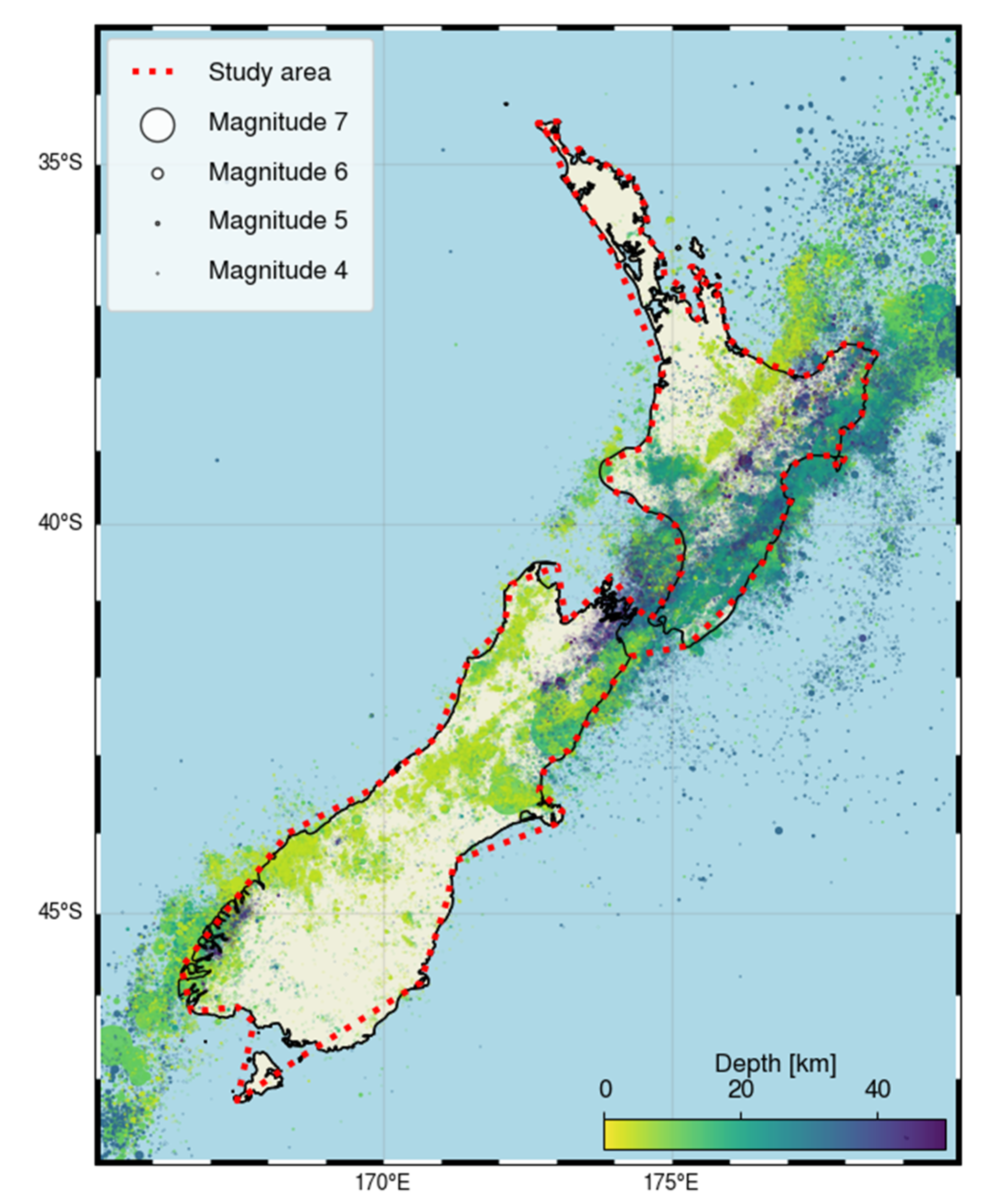
Figure 3.
Orthogonal regression between magnitude scales listed in GeoNet Quake Search system and ML from the revised earthquake catalogue for New Zealand [61]. Both M and MLv fit the data approximately 1:1.
Figure 3.
Orthogonal regression between magnitude scales listed in GeoNet Quake Search system and ML from the revised earthquake catalogue for New Zealand [61]. Both M and MLv fit the data approximately 1:1.
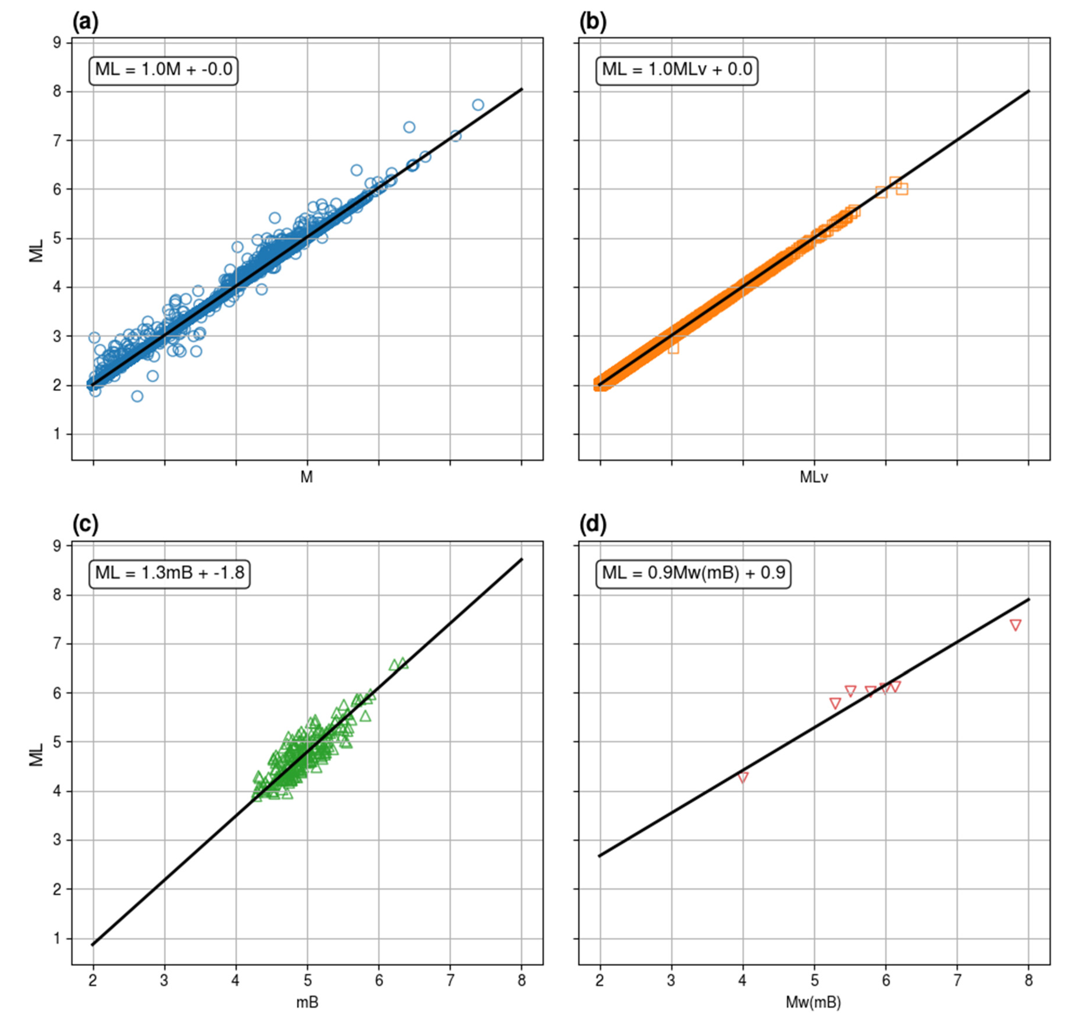
Figure 4.
Completeness magnitude of the catalogue in space.
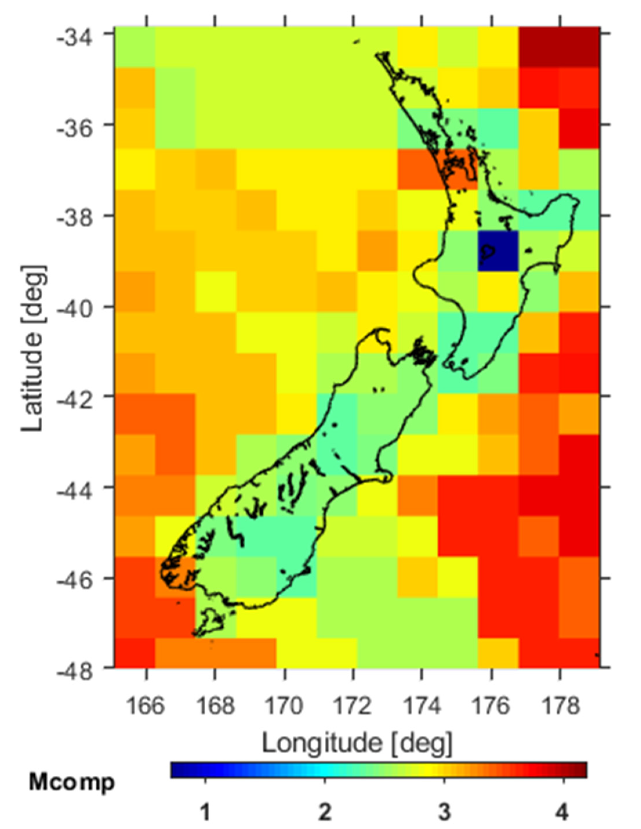
Figure 5.
Test set in the three analyzed cases: (a) chronological; (b) k-fold; (c) autotest. The black arrow in (b) marks the September 2010 Canterbury earthquake.
Figure 5.
Test set in the three analyzed cases: (a) chronological; (b) k-fold; (c) autotest. The black arrow in (b) marks the September 2010 Canterbury earthquake.
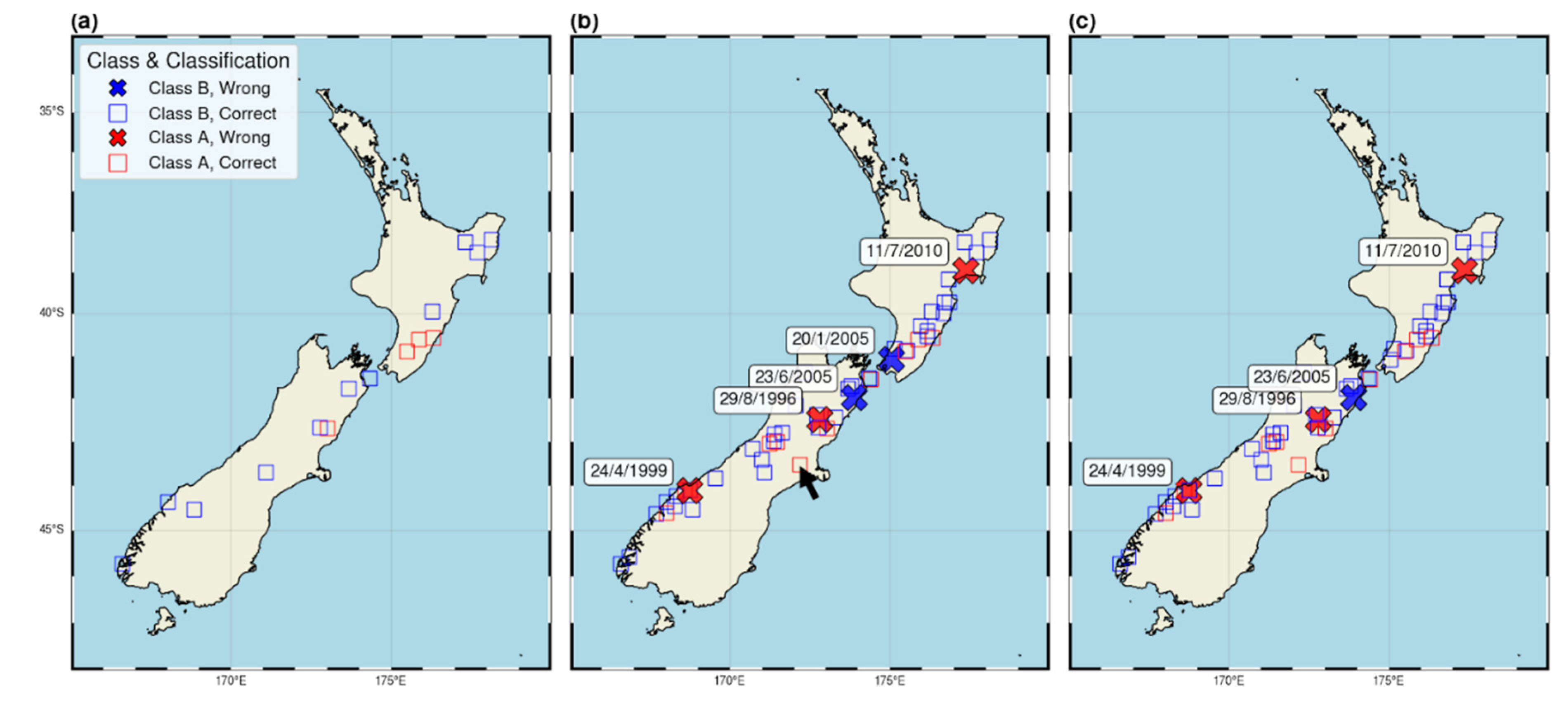
Figure 6.
ROC diagram in the (a) chronological, (b) k-fold, and (c) autotest approach. The Time interval end is expressed in fraction of day.
Figure 6.
ROC diagram in the (a) chronological, (b) k-fold, and (c) autotest approach. The Time interval end is expressed in fraction of day.
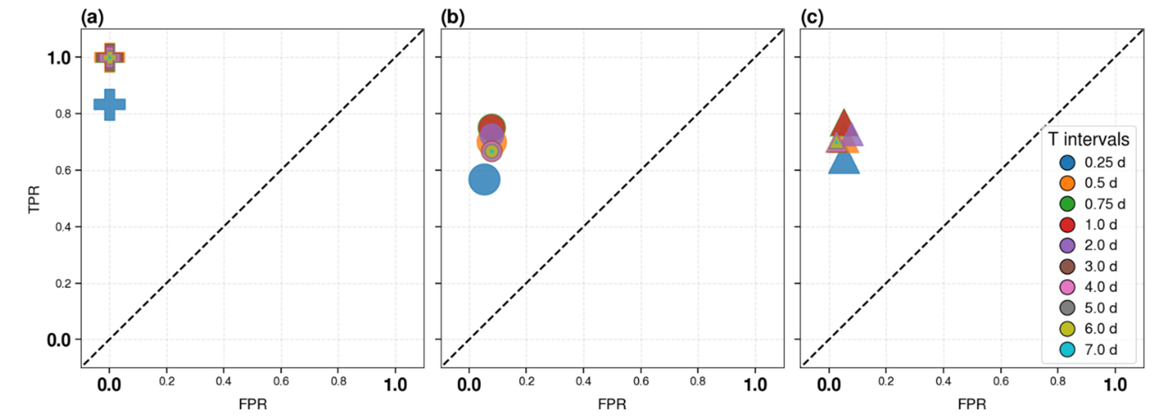
Figure 7.
Precision-Recall diagrams for the (a) chronological, (b) k-fold, and (c) autotest approaches.
Figure 7.
Precision-Recall diagrams for the (a) chronological, (b) k-fold, and (c) autotest approaches.
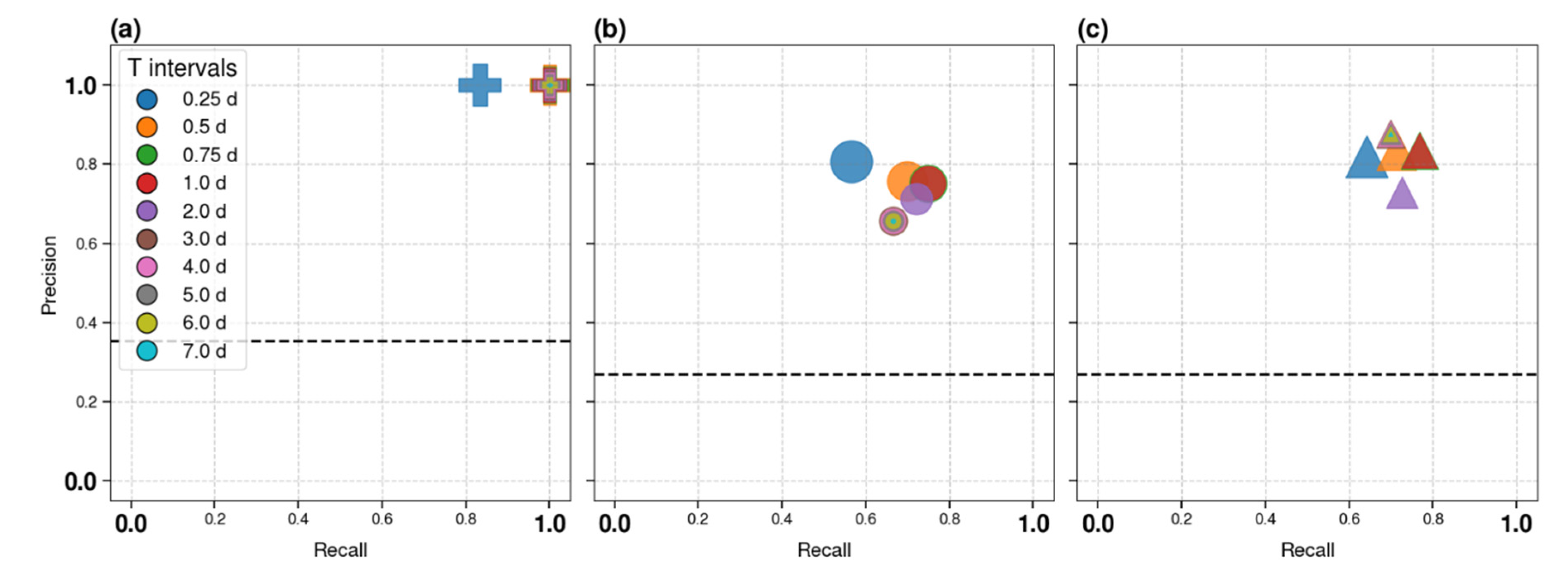
Figure 8.
Comparison of features thresholds in the different regions: (a) S; (b) Z; (c) SLCum; (d) QLCum; (e) SLCum2; (f) QLCum2; (g) Q; (h) Vm; (i) N2. Adapted from Gentili et al. [44].
Figure 8.
Comparison of features thresholds in the different regions: (a) S; (b) Z; (c) SLCum; (d) QLCum; (e) SLCum2; (f) QLCum2; (g) Q; (h) Vm; (i) N2. Adapted from Gentili et al. [44].
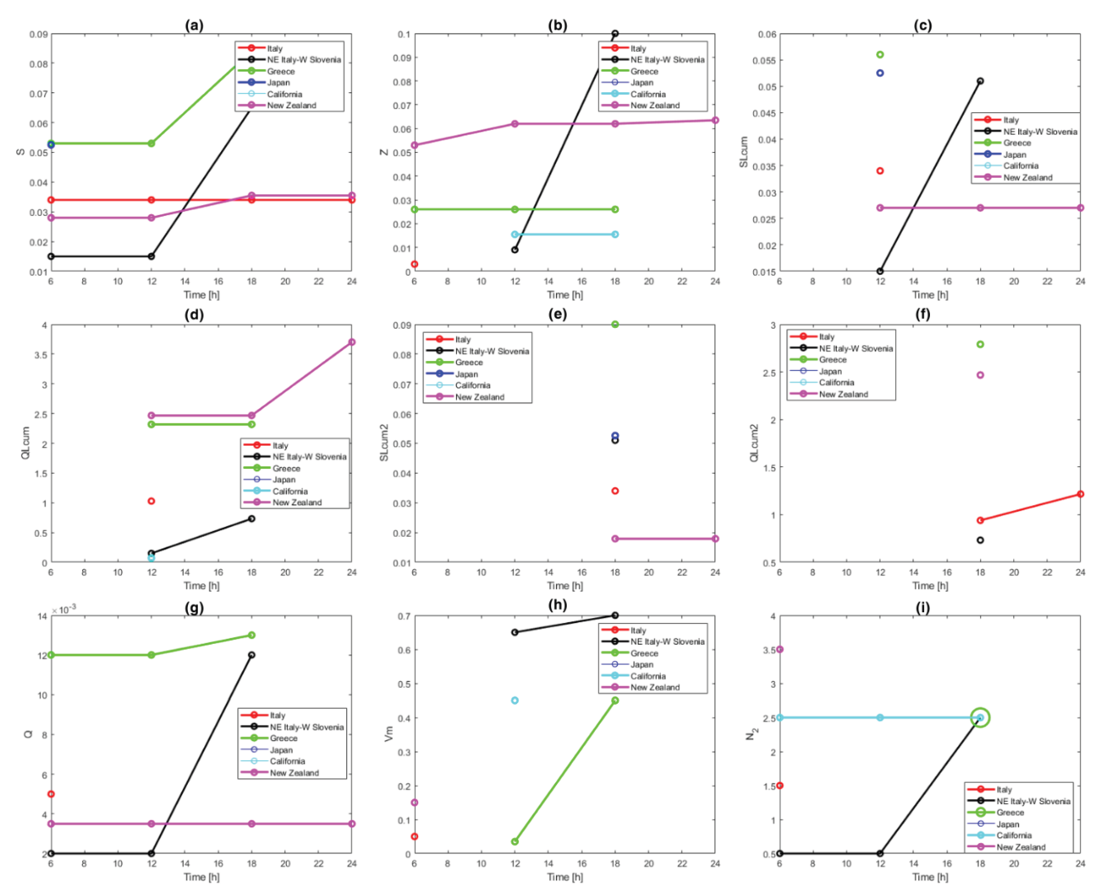

Table 1.
Orthogonal regressions parameters.
| Magnitude | Slope | Std Error | Intercept | Std Error |
|---|---|---|---|---|
| M | 1.006 | 0.0001 | -0.0147 | 0.0003 |
| MLv | 0.9994 | 0.0003 | 0.001 | 0.001 |
| mB | 1.30 | 0.05 | -1.7 | 0.2 |
| Mw(mB) | 0.87 | 0.08 | 0.9 | 0.4 |
Table 2.
Seismicity features adopted by NESTORE.
| Feature | Definition | Type |
|---|---|---|
| Number of events (N2) |
(1) | Space-Time distribution of events |
| Linear Concentration of Events (Z) |
||
| Normalized event source area (S) | Source area and Magnitude trends over time | |
| Cumulative deviation of S from the long-term trend on increasing length windows (SLCum) |
||
| Cumulative deviation of S from the long-term trend on sliding windows (SLCum2) |
] | |
| Cumulative variation of magnitude from event to event (Vm) |
||
| Normalized radiated Energy (Q) |
Energy trends over time | |
| Cumulative deviation of Q from the long-term trend on increasing length windows (QLcum) |
||
| Cumulative deviation of Q from the long-term trend on sliding windows (QLCum2) |
] |
(1) H = Heaviside step function; mi = magnitude of the ith event. (2) rij = distance between the ith and jth events. (3) Em = mainshock energy; Ei = the energy of the ith event.
Table 3.
Training and testing datasets selected following the chronological, the k-fold cross-validation method and the autotest approach. The actual training sets are the ones without outliers.
Table 3.
Training and testing datasets selected following the chronological, the k-fold cross-validation method and the autotest approach. The actual training sets are the ones without outliers.
| Method | Dataset | |||||||
|---|---|---|---|---|---|---|---|---|
| Training | Testing | |||||||
| Subset | N clus | N A | N B | Subset | N clus | N A | N B | |
| Chronological | 1988-2013 | 35 | 8 | 27 | 2014-2025 | 15 | 4 | 11 |
| Without outliers | 33 | 6 | 27 | |||||
| k-fold, k=3 | k-f2 + k-f3 | 35 | 9 | 26 | k-f1 | 17 | 5 | 12 |
| Without outliers | 32 | 6 | 26 | |||||
| k-f1 + k-f3 | 34 | 9 | 25 | k-f2 | 18 | 5 | 13 | |
| Without outliers | 31 | 6 | 25 | |||||
| k-f1 + k-f2 | 35 | 10 | 25 | k-f3 | 17 | 4 | 13 | |
| Without outliers | 33 | 8 | 25 | |||||
| Autotest | All | 52 | 14 | 38 | All | 52 | 14 | 38 |
| Without outliers | 48 | 10 | 38 | |||||
Table 4.
Values of α for each of the three approaches.
| Method | α x 100% |
|---|---|
| Chronological | 0.9840 |
| K-fold | 0.0151 |
| autotest | 0.0072 |
Table 5.
Thresholds obtained by training with the entire dataset. The bold values are calculated for the corresponding time interval, while the others are inherited from the previous intervals.
Table 5.
Thresholds obtained by training with the entire dataset. The bold values are calculated for the corresponding time interval, while the others are inherited from the previous intervals.
| Feature | 6h | 12h | 18h | 1d | 2d | 3d |
|---|---|---|---|---|---|---|
| S | 0.028 | 0.028 | 0.0355 | 0.0355 | 0.0355 | 0.096 |
| Z | 0.053 | 0.062 | 0.062 | 0.0635 | 0.0635 | 0.0635 |
| SLcum | - | 0.027 | 0.027 | 0.027 | 0.055 | 0.1695 |
| QLcum | - | 2.468 | 2.468 | 3.702 | 3.702 | 3.702 |
| SLcum2 | - | - | 0.017901 | 0.017901 | 0.027565 | 0.027565 |
| QLcum2 | - | - | 2.468 | 2.468 | 2.468 | 2.468 |
| Q | 0.0035 | 0.0035 | 0.0035 | 0.0035 | 0.004 | 0.004 |
| Vm | 0.15 | 0.15 | 0.15 | 0.15 | 0.15 | 0.15 |
| N2 | 3.5 | 3.5 | 3.5 | 3.5 | 3.5 | 3.5 |
Disclaimer/Publisher’s Note: The statements, opinions and data contained in all publications are solely those of the individual author(s) and contributor(s) and not of MDPI and/or the editor(s). MDPI and/or the editor(s) disclaim responsibility for any injury to people or property resulting from any ideas, methods, instructions or products referred to in the content. |
© 2025 by the authors. Licensee MDPI, Basel, Switzerland. This article is an open access article distributed under the terms and conditions of the Creative Commons Attribution (CC BY) license (http://creativecommons.org/licenses/by/4.0/).
Copyright: This open access article is published under a Creative Commons CC BY 4.0 license, which permit the free download, distribution, and reuse, provided that the author and preprint are cited in any reuse.


