
Submitted:
24 November 2025
Posted:
26 November 2025
You are already at the latest version
Abstract
Speaker change detection (SCD) in long, multi-party meetings is essential for diarization, ASR, and summarization, and is now often performed in the space of pre-trained speech embeddings. However, unsupervised back-ends remain dominant when timely labeled audio is scarce, and their behavior under a unified modeling setup is still not well understood. In this paper, we systematically compare two representative unsupervised approaches on the multi-talker audio meeting corpus: (i) a clustering-based single-scale pipeline that segments and clusters embeddings/features and scores boundaries via cluster changes and jump magnitude, and (ii) a multi-scale jump-based detector that measures embedding discontinuities at several window lengths and fuses them by temporal clustering and voting. Using a shared front-end and protocol, we vary the underlying features (ECAPA, WavLM, wav2vec 2.0, MFCC, log-Mel) and test robustness under additive noise. Results show that embedding choice is crucial and that the two methods offer complementary trade-offs: the pipeline yields low false alarm rates but higher misses, while the multi-scale detector achieves relatively high recall at the cost of many false alarms.
Keywords:
speaker change detection
; unsupervised learning
; clustering
; embedding
1. Introduction
Speaker change detection (SCD) aims to locate time points at which the active speaker changes in a recording. Reliable SCD is a key building block for downstream applications such as speaker diarization, meeting transcription, and summarization, especially for long and multi-party conversations.
With the advent of powerful pre-trained speech encoders (e.g., ECAPA-TDNN [24], wav2vec 2.0 [10], WavLM [19]), it has become natural to formulate SCD in an embedding space, where each short audio block is mapped to a high-level representation capturing speaker and phonetic information.
However, the most practical diarization and SCD systems typically rely on pre-trained neural speaker embeddings combined with an unsupervised back-end, such as agglomerative or spectral clustering and resegmentation [20,21]. For speaker change detection, a large portion of recent work still adopts unsupervised segmentation criteria—e.g., BIC- or distance-based statistics over frame/block-level features—often coupled with simple clustering heuristics [16,23]. In parallel, supervised and end-to-end SCD models [13,22] built on top of self-supervised speech encoders have begun to emerge, but they are not yet as ubiquitous in practical pipelines.
For SCD, two families of unsupervised methods are particularly popular. The first family detects local jumps or novelty peaks in the embedding sequence, often using spectral flux–style measures and sometimes combining multiple time scales (multi-scale novelty detection). The second family builds segment-level structure by clustering block embeddings into pseudo-speaker states and then applying simple sequence models such as hysteresis thresholding or Viterbi decoding. Both approaches encode different structural priors about how speakers change over time, and both are attractive because they avoid supervised training on time-stamped change labels.
Despite their wide use, these methods are usually proposed and evaluated in isolation: different works rely on different embedding back-ends, datasets, tolerances, and hyperparameters. As a result, it is difficult to answer several basic but practically important questions:
- Under a common setup, how do multi-scale jump detectors compare to clustering-based pipelines?
- How sensitive are these methods to the choice of embedding (ECAPA, WavLM, wav2vec2, MFCC, log-Mel)?
In this work, we focus on revisiting two representative unsupervised approaches under a unified framework and provide a systematic empirical study on the AMI meeting corpus. All methods share the same block segmentation and pre-trained embeddings; we vary only the structural prior (multi-scale jump vs. clustering-based pipeline) and the type of embedding. This controlled setting allows us to directly attribute performance differences to the segmentation strategy and feature choice, rather than to confounding factors.
The main contributions are three-fold:
- Unified comparison of two structural priors. We implement a multi-scale jump detector and a clustering-based single-scale pipeline on top of the same pre-trained embeddings, and compare them under identical evaluation protocols (tolerance, metrics, and datasets).
- Feature and embedding study. We systematically evaluate both methods with ECAPA, WavLM, wav2vec 2.0, MFCC, and log-Mel features, and analyze how the choice of embedding affects detection accuracy and the trade-off between missed detections and false alarms.
- Practical insights and guidelines. Based on the experiments, we highlight when multi-scale detection can match the pipeline (e.g., with strong ECAPA embeddings) and when it collapses, and we summarize concrete recommendations for method and hyperparameter selection in real-world SCD systems.
By focusing on analysis rather than proposing a new algorithm, this study offers a clearer understanding of how current unsupervised SCD methods behave in a realistic setting, and provides a solid baseline and design guide for future supervised or semi-supervised approaches.
2. Related Work
Early unsupervised SCD methods assumed parametric distributions for short windows on either side of a candidate boundary and used generalized likelihood or model selection tests to decide if a change occurred. A foundational line of research models epstral features with Gaussians/GMMs and compares the “one-segment” vs. “two-segment” hypotheses via the Bayesian Information Criterion (BIC), often in a window-growing or divide-and-conquer scheme [1,2,3]. These approaches are simple and annotation-free, but can be sensitive to thresholding, covariance estimation, and window sizing; in practice, peak picking and non-maximum suppression (NMS) are commonly added to reduce duplicate triggers [1,2].
To avoid fragile parametric assumptions, nonparametric distribution-shift tests have been adopted. The maximum mean discrepancy (MMD) offers a kernel-based two-sample test with linear-time variants and strong theoretical guarantees [4]. Complementary work estimates density ratios directly (e.g., uLSIF/RuLSIF ) to quantify segment mismatch without separately estimating each density [5,6]. Distance-based energy statistics provide another assumption-light route and have been used for change-point analysis in multivariate settings [7,8].
Some studies cast SCD as a segmentation problem solvable with dynamic programming or as HMM/HSMM-style modeling, sometimes coupled with BIC validation or DP search to enforce global consistency of cuts under a segment-cost objective [1].
With the advent of i/x-vector style embeddings, SCD can be driven by abrupt changes in embedding space (e.g., cosine or PLDA distance spikes) or by inconsistencies in online clustering assignments. Although developed for speaker recognition, x-vectors became standard building blocks within diarization/SCD pipelines and improved robustness under domain shift [9].
Recent self-supervised encoders provide stronger low-label representations for boundary detection: wav2vec 2.0 [10], HuBERT [11], and WavLM [19] yield frame/segment embeddings that better capture speaker and prosodic cues. In unsupervised SCD, these embeddings are typically frozen (or lightly tuned) and paired with distributional tests or distance-based scoring, often requiring dimensionality reduction/whitening and robust normalization.
When ASR transcripts are available, lexical signals—e.g., pause durations, punctuation/turn markers, and topical or lexical shifts—can complement acoustic evidence. Neural architectures that fuse lexical and acoustic streams show gains over purely acoustic, BIC-style baselines, even with imperfect ASR [12,13].
Most systems apply smoothing, minimum-segment-length constraints, hysteresis/double thresholds, and NMS. SCD-style evaluation commonly reports miss detection rate, false alarm rate with precision/recall/F1 under a tolerance collar around reference boundaries, while diarization-style evaluations emphasize DER/JER; for example, DIHARD II standardized DER/JER and (notably) used no collar in its official scoring, whereas other works adopt fixed collars (e.g., 0.25 s) depending on corpus and protocol [14,15].
In summary, BIC/GLR offer strong low-complexity baselines; kernel tests and density-ratio estimation mitigate distributional mismatch; embedding- and SSL-based features boost separability; and lexical fusion helps in noisy acoustics.
3. Methodology
3.1. Problem Formulation & Notation
We consider the task of speaker change detection on long conversational recordings. Given an input waveform sampled at , the goal is to predict a set of boundary times at which the underlying speaker identity changes.
During evaluation, a predicted boundary is counted as correct if it lies within seconds of any reference change point, with unless otherwise stated.
3.2. Acoustic Embeddings
Both methods are built upon a common foundation: high-dimensional acoustic embeddings. The audio is first segmented into overlapping blocks (e.g., 0.8-second windows with a 0.4-second hop). An embedding model is then used to extract a feature vector for each block. The system supports several pluggable backends:
- Log-Mel: Standard mean and standard deviation of log-mel spectrogram frames.
- MFCC: Mel-Frequency Cepstral Coefficients, a classic acoustic feature derived from the log-mel spectrogram.
- ECAPA-TDNN: A speaker-recognition model that provides a robust, fixed-dimension speaker embedding.
- WavLM: A large-scale pre-trained model that captures rich acoustic and speaker characteristics.
- wav2vec2: Another large-scale pre-trained model that captures contextual speech representations.
These block-level vectors form the time-series data used for all subsequent analyses.
3.3. Pipeline: Clustering-Based Approach
3.3.1. Single-Scale Seeding and Segmentation
The first stage operates on a single time scale defined by the block length w and hop size h. From the normalized jump curve we perform 1-D peak picking with a minimum distance of blocks and a data-dependent threshold (e.g., a fixed upper quantile) to obtain an initial set of candidate boundaries in block indices . These peaks partition the recording into contiguous segments , where each segment spans all blocks between two consecutive peaks.
3.3.2. Segment-Level Embeddings and Clustering
For each segment , we compute a segment-level embedding by averaging the block embeddings within the segment. The sequence is then clustered using an unsupervised algorithm (e.g., agglomerative clustering with a distance threshold). The resulting cluster labels can be interpreted as pseudo-speaker or pseudo-topic identities.
To avoid spurious short segments, we apply a simple temporal smoothing on the cluster labels, enforcing a minimum run length in the segment index domain.
3.3.3. Boundary Scoring and Decoding
For each boundary between consecutive segments , we define two scalar features:
i) a segment boundary jump
where and denote the last block of and the first block of , respectively;
ii) a cluster change indicator
encoding whether the segment-level cluster label changes.
After normalization, we combine these into a single boundary score
with fixed weights . The sequence is then decoded into a set of final change points using a 1-D hysteresis thresholding scheme with a high and low threshold and a minimum segment duration constraint (or equivalently, a two-state HMM with Viterbi decoding).
3.4. Multi-Scale Jump-Based Detector
3.4.1. Single-Scale Jump Curves at Multiple Time Scales
The multi-scale detector uses the same embedding model but operates at multiple analysis scales. We define a set of window lengths
(e.g., 0.4, 0.8, and 1.6 seconds) and, for each scale , segment the waveform into blocks of length s with a hop size of .
At each scale we compute block embeddings and a corresponding jump curve . Local maxima are detected on using a minimum distance and percentile-based height threshold, yielding a set of candidate change points with associated confidence scores
3.4.2. Cross-Scale Fusion by Clustering and Voting
All candidate times from all scales are pooled and sorted to obtain a combined set
where denotes the originating scale. We then apply a simple temporal clustering: starting from the earliest time, we group candidates whose timestamps lie within a fixed window (e.g., 0.2 s) into the same cluster.
For each cluster , we compute a scale agreement score
and a confidence score given by the mean (or max) of over the cluster.
A cluster is accepted as a change point if both the scale agreement and confidence exceed fixed thresholds (e.g., and ). The final boundary time is taken as the average timestamp of the cluster members.
4. Experiments
4.1. Dataset
Table 1 reports per-recording statistics on the DEV split. We show the recording duration (in seconds), the number of annotated speaker-change boundaries (“#Boundaries”), and the boundary density in boundaries per minute (“Boundaries/min”). DEV contains 18 meetings ranging from ∼944 s to 2,970 s. Boundary density spans 6.6–20.6/min, with IS1008b being the least conversationally active (6.62/min) and IB4010 the most (20.55/min). This spread reflects substantial heterogeneity across sessions, which we use to tune hyperparameters and check robustness.
Table 2 lists the same statistics for the TEST split (16 meetings). Durations range from ∼839 s to 2,972 s. Boundary density is generally higher and broader than DEV, spanning 7.5–28.7/min: TS3003c is the calmest (7.54/min), while EN2002a is the most dynamic (28.70/min). The mixture of relatively quiet and highly interactive meetings makes this split a good stress-test for change-point detectors.
4.2. Evaluation Metrics
To evaluate the performance of speaker change point detection, a detected boundary is considered correct if it falls within a specified time tolerance (or "collar") around a ground-truth boundary. A standard tolerance of seconds is used unless otherwise specified. We also report sensitivity at
To assess the performance of the approaches, several metrics are employed:
i)The missed detection rate (MDR) measures the ratio of missed speaker-change boundaries to the total number of ground-truth boundaries:
ii) The false alarm rate (FAR) measures the proportion of incorrect speaker-change detections, calculated as the ratio of false positives to all non-change points:
Additionally, precision is used to indicate the accuracy of detected speaker changes, recall (Hit-rate) assesses the ability to identify all true speaker changes, and the F1 score provides a balanced measure of precision and recall.
4.3. Experimental Design
Experiments are conducted on a standard benchmark dataset (the AMI Corpus) to ensure reproducible results. All hyperparameters are tuned on the Dev split and kept fixed on Test set.
4.4. Experiment 1: Acoustic Embedding Comparison
The goal of this experiment is to identify the most effective acoustic embedding for the segmentation task. We adopt the Pipeline (Single-Scale Clustering Pipeline) as a fixed evaluation framework because it exercises all components of the system—seeding, clustering, and Viterbi decoding—thereby providing a comprehensive assessment of feature quality. Five embedding types are considered: Log-Mel, MFCC, ECAPA-TDNN, WavLM, and wav2vec2. For fairness, all non-feature hyperparameters (e.g., clustering algorithm and Viterbi weights) are held constant across runs. Performance is measured by the F1-score at a tolerance of . The two best-performing embeddings under this criterion are selected for subsequent analyses.
4.5. Experiment 2: Evaluation Tolerance Sweeping
To characterize the tolerance sensitivity of the best-performing features, we run a tolerance sweep using the ECAPA-based Pipeline. Specifically, we evaluate the system at three collar widths, . For each tolerance, we compute Precision, Recall, and F1-score and compare how these metrics change as the collar widens. This analysis highlights which embedding is more accurate at tight boundary localization (small t) and which maintains more stable performance when near-miss detections are gradually forgiven (larger t).
4.6. Experiment 3: Clustering Method Comparison
This experiment evaluates the impact of different clustering algorithms within the pipeline, using the best-performing ECAPA-TDNN embedding. The clustering module is exchanged among the available algorithms, including Agglomerative, Spectral and DBSCAN, while all other components and hyperparameters remain unchanged. We report the F1-score at for each method to quantify the influence of clustering choice on final detection accuracy.
4.7. Experiment 4: Analysis of Multi-Scale Settings
To better understand the behavior of the multi-scale detector, we conduct an ablation study on the choice of analysis scales and fusion strategy on dev set. Concretely, we compare (i) a single-scale baseline using a window length of 0.8 s, (ii) two-scale variants combining 0.4+0.8 s and 0.8+1.6 s, and (iii) the full three-scale configuration 0.4+0.8+1.6 s used in our main experiments. The three window lengths are chosen to roughly cover short, medium, and long conversational units within meetings: 0.4 s is sensitive to rapid local changes (e.g., short backchannels), 0.8 s corresponds to typical short turns, and 1.6 s captures slower, more sustained speaker or topic shifts. This design allows us to test whether adding more scales always helps.
4.8. Experiment 5: Final Pipeline Comparison
Finally, we compare the two complete SCD approaches introduced in Section 3 on test set: (i) the clustering-based Pipeline, configured with the best-performing embedding and clustering combination identified in Experiments 1 and 3 (ECAPA-TDNN with constrained agglomerative clustering) on dev set; and (ii) the Multi-scale jump-based detector using the same ECAPA embedding and evaluation protocol.
We evaluate Precision, Recall, and F1-score at a tolerance of for both approaches on the AMI test splits to quantify their overall performance trade-offs.
4.9. Experiment 6: Evaluate Robustness
We further assess the robustness of the two unsupervised SCD methods under noisy conditions that approximate realistic deployment scenarios. Starting from the original AMI meeting dev recordings, we create three noisy test sets corresponding to low, medium, and high noise levels by adding zero-mean white Gaussian noise to the waveform. For each recording, the noise is generated and scaled according to a predefined noise-to-signal power ratio (higher levels correspond to stronger noise) and then added sample-wise, with the resulting signal clipped to the range if necessary. For each noise level, we run both the clustering-based pipeline and the multi-scale detector with exactly the same hyper-parameters as in the clean setting, and evaluate them using the standard metrics (Precision, Recall, F1, MDR, FAR) at a 0.5 s tolerance. This setup allows us to quantify how each method trades off missed detections and false alarms as background noise increases, and to judge their suitability for real-world meeting scenarios with varying degrees of acoustic corruption.
5. Results
5.1. Results of Acoustic Embedding Comparison
Table 3 summarize the results of the pipeline on the development set with a 0.5s tolerance. The ECAPA-TDNN embedding achieved a significantly higher F1-Score (33.61) than all other features, driven by strong P (34.35) and R (32.89). WavLM was the clear runner-up, while the classic acoustic features (MFCC, Log-Mel) and the general-purpose wav2vec2 model showed considerably lower performance, particularly in recall.
We hypothesize that ECAPA-TDNN works best because it makes “steady” features for the same speaker/scene and shows a clear jump only when the speaker/scene really changes.
MFCC is more sensitive to small sound changes (like loudness or phonemes), so it fires inside segments and breaks them up. WavLM/wav2vec2 focus more on speech content (words/phones), so they often react at word changes and, with their heavy context smoothing, can blur real speaker changes unless fine-tune them for speaker cues.
Table 4 presents feature comparison results of the multi-scale approach on development set. It can be observed, on the dev set (tol = 0.5 s), the multi-scale detector works best with the ECAPA embedding, reaching 33.7% F1 with a relatively balanced precision (28.8%) and recall (40.4%). In contrast, WavLM achieves lower F1 (20.4%) and much lower recall, while wav2vec2, MFCC, and Log-Mel almost collapse in recall (< 2%), giving very low F1 despite low false alarm rates. This indicates that the effectiveness of the multi-scale method is highly dependent on the embedding, and ECAPA provides the most suitable representation in the current setting.
Figure 1 shows that the clustering-based Pipeline outperforms the Multi-scale detector for most feature types. With ECAPA embeddings the two methods are almost tied (both ≈ 34% F1), but for WavLM, wav2vec2, MFCC, and Log-Mel the Pipeline is clearly better, while the Multi-scale detector almost collapses for wav2vec2/MFCC/Log-Mel (F1 ≈ 1–4%). This indicates that the Pipeline peforms well across different embeddings, whereas the Multi-scale method only works well when the embedding (ECAPA) already provides very strong speaker-discriminative structure.
Under the same cluster (Agglomerative) and evaluation tolerance (0.5 s), ECAPA features significantly outperformed other custom/handcrafted features for both approaches.
Based on this, we used ECAPA+Agglomerative as the primary configuration for subsequent development and test set validation, using WavLM/MFCC/Log-Mel as the baseline to ensure that the improvement was due to the algorithm rather than randomness of the features.
5.2. Results for Tolerance Sweeping
We compare the pipeline baseline with the multi–scale detector under different collar tolerances (0.25/0.5/0.75 s). The results are presented in Table 5. At the strict 0.25s collar, the pipeline clearly outperforms the multi–scale variant in terms of precision, recall and F1 (23.17% vs. 15.93%), while also achieving a lower false alarm rate (5.19% vs. 8.60%), indicating a more conservative and cleaner segmentation. At the standard 0.5s collar, both systems obtain almost identical F1 scores (33.6%), but the multi–scale detector achieves a substantially higher recall (+7.6 pp, 40.44% vs. 32.89%) at the cost of a higher FAR (+5.9 pp). With a more relaxed 0.75s collar, the multi–scale approach further improves F1 (42.12% vs. 39.44%) and recall (50.58% vs. 38.60%), again trading off against an increased FAR (23.65% vs. 15.08%). Overall, the multi–scale detector is more recall–oriented and tends to over–segment, whereas the pipeline baseline is more conservative with fewer false alarms.
Figure 2 illustrates how the pipeline baseline and the multi–scale detector behave under different collar tolerances (0.25 s, 0.5 s, 0.75 s). As the tolerance increases, both approaches gain recall but also incur higher FAR. The multi–scale detector achieves higher recall than the pipeline, especially at 0.5 s and 0.75 s, but at the cost of more false alarms, while the pipeline remains more conservative with lower FAR.
5.3. Result with Various Clustering Algorithms
Experiment 3 evaluated the impact of different clustering algorithms within the Baseline pipeline, using the best-performing ECAPA-TDNN embedding. As shown in Table 6, the choice of algorithm is critical to the pipeline’s performance.
The Constrained Agglomerative Clustering method was the only effective algorithm, achieving an F1-Score of 33.61. This result was stable across various distance thresholds (0.55 to 0.65). In sharp contrast, both Spectral Clustering and DBSCAN failed catastrophically. While they achieved high precision (37.32% and 37.03%), their recall was exceptionally low (11.21% and 2.02%, respectively). This indicates that these methods are far too conservative for this task, correctly identifying a few boundaries but missing the vast majority, rendering them unsuitable for this pipeline.
5.4. Results of Analysis of Multi-Scale Settings
Table 7 summarizes an ablation on the choice of analysis scales for the ECAPA-based multi-scale detector on the dev set (tol = 0.5 s). Using a single scale of 0.8 s already gives a reasonably balanced operating point (F1 = 35.6%) with moderate recall (44.4%) and a relatively low false alarm rate (FAR = 16.7%). Adding a shorter 0.4 s scale (0.4+0.8) dramatically boosts recall to 83.3% but at the cost of a relatively high FAR (51.5%), indicating that the additional sensitivity mainly manifests as many extra false positives. Using a longer auxiliary scale (0.8+1.6) yields a more conservative detector with slightly lower F1 (33.3%) and higher FAR than the single-scale baseline. The full three-scale configuration (0.4+0.8+1.6) sits between these extremes: it slightly reduces F1 compared to the best single-scale setting, but achieves the lowest FAR (15.9%), suggesting that the additional scales act more as a regularizer that trades some recall for fewer false alarms.
5.5. Results on Test Set
Table 8 reports per-recording performance for the clustering-based Pipeline and the Multi-scale detector on the test set (tol = 0.5 s). Overall, the Pipeline operates in a more conservative regime: it achieves higher average precision (34.9% vs. 20.4%) and slightly higher average F1 (34.4% vs. 32.1%), with a much lower average false alarm rate (FAR 10.0% vs. 50.0%). In contrast, the Multi-scale method aggressively favors recall, reaching an average recall above 82% on all recordings, which corresponds to a much lower missed detection rate (MDR 17.5% vs. 64.6% for the Pipeline), but this comes at the cost of relatively high false alarm rates on almost every file. Per-file results show the same pattern : the Multi-scale detector substantially increases recall and reduces MDR on all meetings, while the Pipeline provides more balanced precision–recall trade-offs and more stable FAR across sessions.
5.6. Results of Robustness
Table 9 summarizes the behavior of the two methods under three noise levels. For Low and Medium noise, the Multi-scale detector keeps relatively high recall (75–85%) but at the price of extremely high false alarm rates (FAR 50–64%), so its overall error is dominated by false positives.
In contrast, the Pipeline operates in a more conservative regime with much lower FAR (about 8–12%) and slightly higher F1 in these two conditions, but its missed detection rate (MDR ≈ 59–73%) is still high, indicating that many true changes are not detected.
Under High noise, both methods become problematic in different ways. The Multi-scale detector reduces FAR to about 16% but its MDR increases to nearly 64%, so the total error remains large even though F1 stays around 28%. The Pipeline almost stops working as a detector: its recall drops to about 0.7% and MDR approaches 99%, meaning that it produces almost no change points at all and the low FAR (≈0.1%) is achieved only because the system rarely fires. From the joint perspective of MDR and FAR, this operating point is clearly undesirable. Overall, as noise increases, the Multi-scale method mainly trades precision for recall, whereas the Pipeline tends to become overly conservative and can fail to function as a useful SCD system under high-noise conditions.
5.7. Comparing with Other Unsupervised Approaches
Table 10 compares our two ECAPA-based models with classic unsupervised SCD baselines from [16] in terms of MDR and FAR (lower is better). All methods are evaluated on the AMI test set. BIC- and KL-based methods with hand-crafted features typically operate around MDR ≈ 39–47% and FAR ≈ 48–60%. Our Pipeline model is very conservative: it achieves a much lower FAR (9.98%) than all BIC/KL systems, but with a high MDR (64.95%). In contrast, the Multi-scale model attains the lowest MDR in the table (18.24%), showing strong sensitivity to changes, at the price of a FAR (49.01%) comparable to the classic unsupervised approaches.
6. Conclusions
In this paper, we study unsupervised speaker change detection in meeting recordings under a unified embedding-based framework. We use a common front-end with block segmentation and pre-trained embeddings to compare two structural paradigms: a clustering-based single-scale pipeline with hysteresis decoding, and a multi-scale jump-based detector that aggregates embedding discontinuities across multiple time scales. Both methods are assessed on the AMI corpus using a consistent protocol for tolerance, evaluation metrics, and data splits.
The experimental study covered several dimensions. First, we performed a feature/embedding comparison for both methods using ECAPA, WavLM, wav2vec 2.0, MFCC, and log-Mel features. Second, we ran a head-to-head comparison of the pipeline and multi-scale detector on dev and test sets, including per-recording analysis. Third, we conducted an ablation on the multi-scale configuration, varying window sets (single-scale 0.8 s, two-scale 0.4+0.8 and 0.8+1.6, and three-scale 0.4+0.8+1.6). Fourth, we evaluated robustness to additive white noise at low, medium, and high levels. Finally, we compared against classic unsupervised SCD baselines (BIC/KL with hand-crafted features) using common MDR/FAR metrics.
The results lead to several key findings. (1) Embedding choice is critical, especially for the multi-scale detector: ECAPA delivers the best F1, while wav2vec2, MFCC, and log-Mel cause the multi-scale approach to almost collapse in recall, whereas the pipeline remains more stable across embeddings. (2) The two methods occupy complementary operating regimes. On test meetings, the pipeline yields higher precision and much lower FAR, but with relatively high MDR; the multi-scale detector achieves relatively high recall (low MDR) at the expense of many false alarms. Per-file results confirm this pattern across all sessions. (3) The multi-scale ablation shows that a single 0.8 s scale already gives strong and balanced performance; adding a shorter 0.4 s scale dramatically boosts recall but drives FAR up, while the three-scale configuration slightly reduces F1 yet delivers the lowest FAR, suggesting that additional scales mainly act as a regularizer that can be tuned to the desired precision–recall trade-off. (4) Under increasing noise levels, both methods become less reliable, but in different ways: for low and medium noise the Multi-scale detector keeps relatively high recall at the cost of extremely high FAR (errors dominated by false alarms), while the Pipeline stays usable with much lower FAR but still high MDR; under high noise the Multi-scale detector loses recall and still has substantial FAR, and the Pipeline almost stops detecting changes at all (near-zero FAR only because almost all true change points are missed). (5) Compared to BIC/KL-based unsupervised SCD with hand-crafted features, the ECAPA-based models can reach substantially lower MDR (multi-scale) or substantially lower FAR (pipeline), showing that modern embeddings plus simple structural priors can outperform classic feature–statistic combinations along different ends of the error trade-off.
These observations suggest several directions for future work. A natural next step is to design hybrid methods that explicitly combine the strengths of both approaches, for example using multi-scale jump cues to propose candidates and the clustering-based pipeline (or a learned classifier) to score and filter them. Another direction is to introduce lightweight supervision or semi-supervised calibration on top of the unsupervised scores, to better control the MDR–FAR trade-off without requiring large amounts of annotated change points. Finally, extending the analysis to more diverse conversational domains and exploring end-to-end architectures that retain the interpretability of jump- and cluster-based features would further bridge the gap between traditional unsupervised pipelines and fully supervised SCD systems.
Author Contributions
Conceptualization, A.T., G.T, B.Z.. ; Methodology, A.T.,G.T. ; Validation, A.T.; Resources, G.T.; Data curation, G.T.; Writing – original draft A.T, G.T.; Writing – review & editing, A.T.; Visualization, G.T.; Project administration, A.T.; Funding acquisition, A.T., B.Z.
Funding
This research was funded by the Committee of Science of the Ministry of Science and Higher Education of the Republic of Kazakhstan under grant number AP19676744.
Data Availability Statement
The data used in this study are publicly available. [https://groups.inf.ed.ac.uk/ami/corpus/] [accessed on 03 March 2024]. The source code for this Speaker Change Detection pipeline is publicly available at [https://github.com/a-toleu/scd_multiscale-pipeline.]
Conflicts of Interest
The authors declare no conflicts of interest.
References
- S. S. Chen and P. S. Gopalakrishnan, “Speaker, environment and channel change detection and clustering via the Bayesian Information Criterion,” in Proc. DARPA Broadcast News Transcription and Understanding Workshop, 1998.
- A. Tritschler and R. A. Gopinath, “Improved speaker segmentation and segments clustering using the Bayesian Information Criterion,” in Proc. EUROSPEECH, 1999.
- Delacourt, P.; Wellekens, C.J. DISTBIC: A speaker-based segmentation for audio data indexing. Speech Communication 2000, 32, 111–126. [Google Scholar] [CrossRef]
- Gretton, A.; Borgwardt, K.M.; Rasch, M.; Schölkopf, J.B.; Smola, A. A kernel two-sample test. Journal of Machine Learning Research 2012, 13, 723–773. [Google Scholar]
- Kanamori, T.; Hido, S.; Sugiyama, M. A least-squares approach to direct importance estimation. Journal of Machine Learning Research 2009, 10, 1391–1445. [Google Scholar]
- Yamada, M.; Suzuki, T.; Kanamori, T.; Hachiya, H.; Sugiyama, M. Relative density-ratio estimation for robust distribution comparison. Neural Computation 2013, 25, 1324–1370. [Google Scholar] [CrossRef] [PubMed]
- Székely, G. J.; Rizzo, M.L. Energy statistics: A class of statistics based on distances. Journal of Statistical Planning and Inference 2013, 143, 1249–1272. [Google Scholar] [CrossRef]
- Rizzo, M.L.; Székely, G.J. Energy distance. Wiley Interdisciplinary Reviews: Computational Statistics 2016, 8, 27–38. [Google Scholar]
- D. Snyder, D. Garcia-Romero, G. Sell, D. Povey, and S. Khudanpur, “X-vectors: Robust DNN embeddings for speaker recognition,” in Proc. ICASSP, 2018, pp. 5329–5333.
- A. Baevski, Y. Zhou, A. Mohamed, and M. Auli, “wav2vec 2.0: A framework for self-supervised learning of speech representations,” in Proc. NeurIPS, 2020.
- W.-N. Hsu, B. Bolte, Y.-H. H. Tsai, K. Lakhotia, R. Salakhutdinov, and A. Mohamed, “HuBERT: Self-supervised speech representation learning by masked prediction of hidden units. IEEE/ACM Transactions on Audio, Speech, and Language Processing 2021, 29, 3451–3460.
- T. J. Park and P. Georgiou, Multimodal speaker segmentation and diarization using lexical and acoustic cues via sequence-to-sequence neural networks. arXiv 2018, arXiv:1805.10731.
- Toleu, A.; Tolegen, G.; Pak, A.; Jaxylykova, A.; Zhumazhanov, B. End-to-End Multi-Modal Speaker Change Detection with Pre-Trained Models. Applied Sciences 2025, 15. [Google Scholar] [CrossRef]
- N. Ryant, K. Church, C. Cieri, A. Cristia, J. Du, S. Ganapathy, and M. Liberman, “The Second DIHARD Diarization Challenge: Dataset, task, and baselines,” in Proc. Interspeech, 2019, pp. 978–982.
- S. Horiguchi, P. S. Horiguchi, P. Garcia, Y. Takashima, S. Watanabe, P. Garcia, and K. Kinoshita, The Hitachi/JHU diarization system for CHiME-6 and DIHARD-II. arXiv 2020, arXiv:2005.09921. [Google Scholar]
- Toleu, A.; Tolegen, G.; Mussabayev, R.; Krassovitskiy, A; Zhumazhanov, B. Comparative Analysis of Audio Features for Unsupervised Speaker Change Detection. Applied Sciences 2024, 14, 12026. [Google Scholar] [CrossRef]
- A. O. T. Hogg, C. Evers, and P. A. Naylor, “Speaker Change Detection Using Fundamental Frequency with Application to Multi-Talker Segmentation,” in Proc. ICASSP 2019 – IEEE International Conference on Acoustics, Speech and Signal Processing (ICASSP), 2019, pp. 5826–5830. [CrossRef]
- T. J. Park, N. Kanda, D. Dimitriadis, K. J. Han, S. Watanabe, and S. Narayanan, A review of speaker diarization: Recent advances with deep learning. Comput. Speech Lang. 2022, 72, 101317. [CrossRef]
- S. Chen, C. Wang, Z. Chen, Y. Wu, S. Liu, Z. Chen, J. Li, N. Kanda, T. Yoshioka, X. Xiao, J. Wu, L. Zhou, S. Ren, Y. Qian, Y. Qian, J. Wu, M. Zeng, X. Yu, and F. Wei, WavLM: Large-Scale Self-Supervised Pre-Training for Full Stack Speech Processing. IEEE Journal of Selected Topics in Signal Processing 2022, 16, 1505–1518. [CrossRef]
- A. Jati and P. Georgiou, “Speaker2Vec: Unsupervised Learning and Adaptation of a Speaker Manifold Using Deep Neural Networks with an Evaluation on Speaker Segmentation,” in Proc. Interspeech 2017, pp. 3567–3571, 2017. [CrossRef]
- A. Jati and P. Georgiou, “An Unsupervised Neural Prediction Framework for Learning Speaker Embeddings Using Recurrent Neural Networks,” in Proc. Interspeech 2018, pp. 1131–1135, 2018. [CrossRef]
- L. Fischbach, “A Comparative Analysis of Speaker Diarization Models: Creating a Dataset for German Dialectal Speech,” in Proceedings of the Third Workshop on NLP Applications to Field Linguistics, Bangkok, Thailand, Aug. 2024, pp. 43–51. [CrossRef]
- VijayKumar, K.; Rajeswara Rao, R. Optimized speaker change detection approach for speaker segmentation towards speaker diarization based on deep learning. Data & Knowledge Engineering 2023, 144, 102121. [Google Scholar] [CrossRef]
- B. Desplanques, J. Thienpondt, and K. Demuynck, “ECAPA-TDNN: Emphasized Channel Attention, Propagation and Aggregation in TDNN Based Speaker Verification,” in Proc. Interspeech, 2020, pp. 3830–3834. [CrossRef]
Figure 1.
Comparison of F1 results on Dev set for the Pipeline vs. Multi-scale.
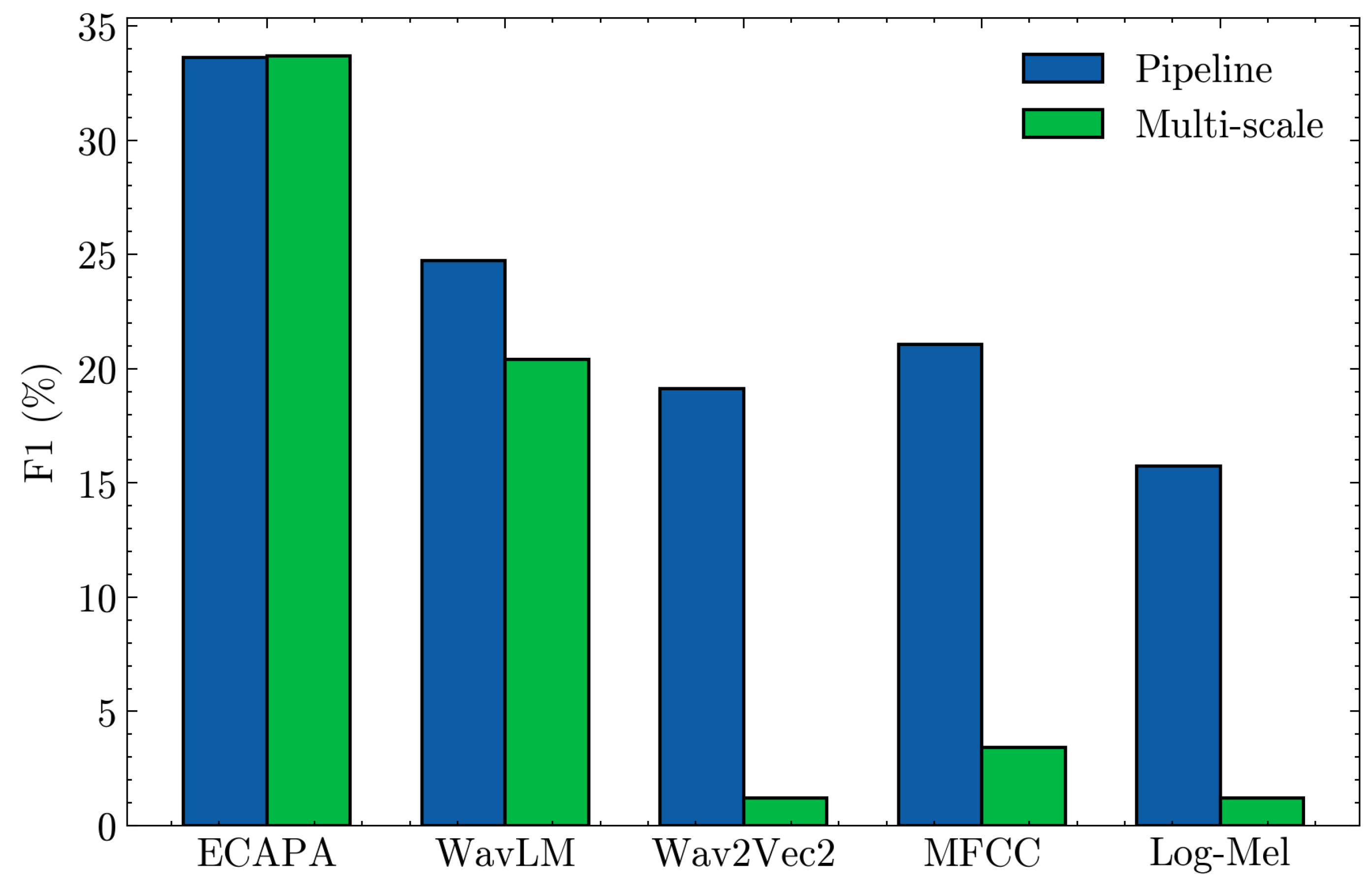
Figure 2.
Recall (top) and false alarm rate (FAR, bottom) versus collar tolerance for the pipeline and multi–scale SCD.
Figure 2.
Recall (top) and false alarm rate (FAR, bottom) versus collar tolerance for the pipeline and multi–scale SCD.
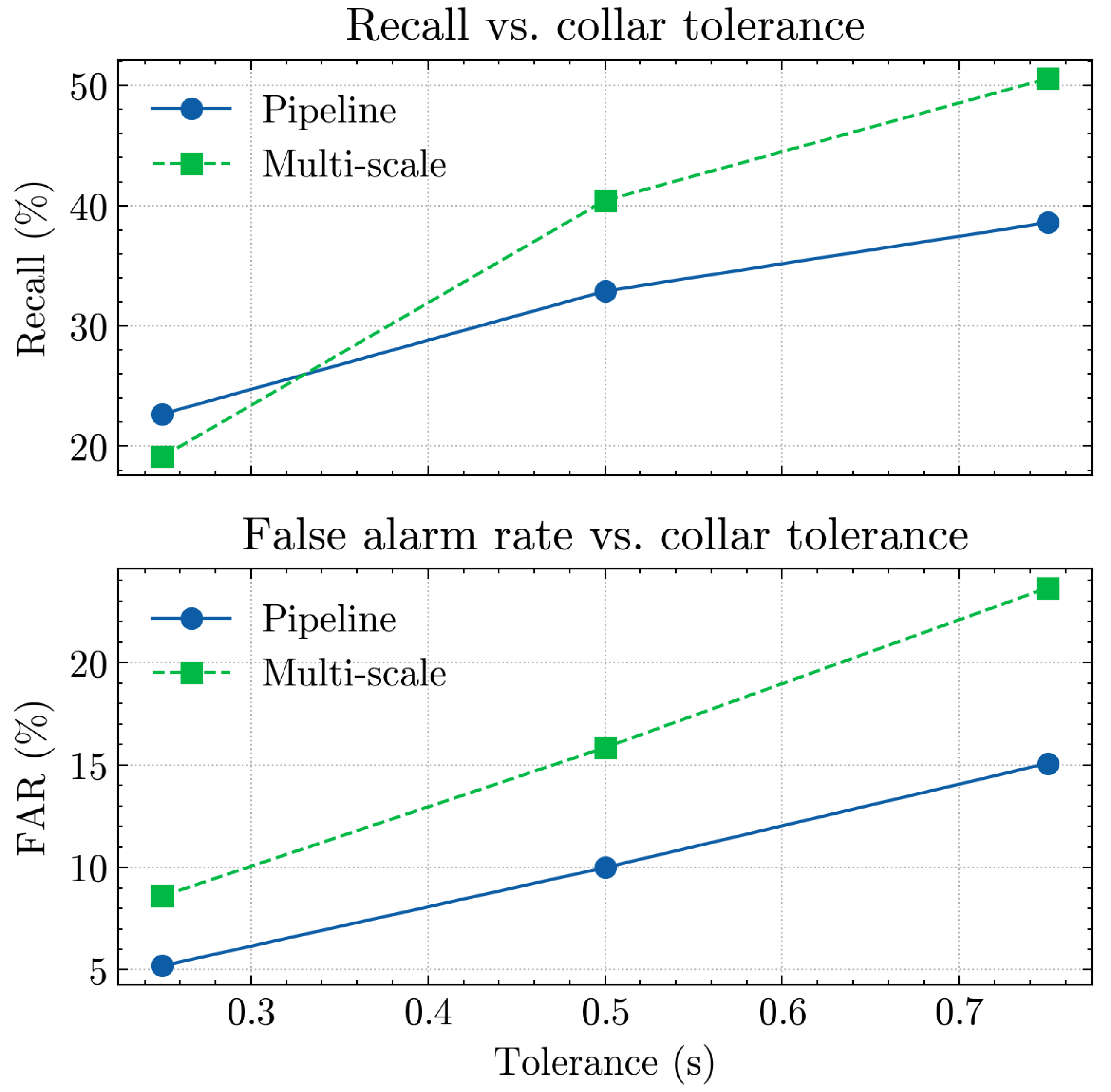

Table 1.
Per-file statistics on the DEV split. Durations in seconds.
| File | Dur. (s) | #Boundaries | Boundaries/min |
| ES2011a | 1113.8 | 217 | 11.69 |
| ES2011c | 1616.1 | 384 | 14.26 |
| IB4001 | 1780.7 | 523 | 17.62 |
| IB4003 | 2023.3 | 486 | 14.41 |
| IB4010 | 2960.6 | 1014 | 20.55 |
| IS1008a | 943.8 | 138 | 8.77 |
| IS1008c | 1546.3 | 205 | 7.95 |
| TS3004a | 1345.3 | 326 | 14.54 |
| TS3004c | 2970.0 | 746 | 15.07 |
| ES2011b | 1581.3 | 325 | 12.33 |
| ES2011d | 1982.3 | 472 | 14.29 |
| IB4002 | 1882.4 | 563 | 17.95 |
| IB4004 | 2392.8 | 634 | 15.90 |
| IB4011 | 2417.0 | 748 | 18.57 |
| IS1008b | 1768.5 | 195 | 6.62 |
| IS1008d | 1480.8 | 322 | 13.05 |
| TS3004b | 2246.1 | 590 | 15.76 |
| TS3004d | 2750.8 | 856 | 18.67 |
Table 2.
Per-file statistics on the TEST split. Durations in seconds.
| File | Dur. (s) | #Boundaries | Boundaries/min | |
| EN2002a | 2142.7 | 1025 | 28.70 | |
| EN2002b | 1786.8 | 660 | 22.16 | |
| EN2002c | 2972.3 | 992 | 20.03 | |
| EN2002d | 2209.9 | 940 | 25.52 | |
| ES2004a | 1049.4 | 247 | 14.12 | |
| ES2004b | 2345.5 | 433 | 11.08 | |
| ES2004c | 2334.4 | 499 | 12.83 | |
| ES2004d | 2222.3 | 628 | 16.96 | |
| IS1009a | 838.8 | 207 | 14.81 | |
| IS1009b | 2052.3 | 424 | 12.40 | |
| IS1009c | 1820.8 | 267 | 8.80 | |
| IS1009d | 1944.5 | 485 | 14.97 | |
| TS3003a | 1505.6 | 201 | 8.01 | |
| TS3003b | 2210.3 | 313 | 8.50 | |
| TS3003c | 2570.0 | 323 | 7.54 | |
| TS3003d | 2618.2 | 666 | 15.26 |
Table 3.
Feature comparison on the dev set (tol = 0.5 s) for the Pipeline.
| Feature | Precision ↑ | Recall ↑ | F1 ↑ | MDR ↓ | FAR ↓ |
|---|---|---|---|---|---|
| ECAPA | 34.35 | 32.89 | 33.61 | 67.11 | 9.99 |
| WavLM | 26.60 | 23.07 | 24.71 | 76.93 | 10.11 |
| wav2vec2 | 26.00 | 15.14 | 19.14 | 84.86 | 6.85 |
| MFCC | 28.23 | 16.80 | 21.07 | 83.20 | 6.79 |
| Log-Mel | 27.72 | 11.00 | 15.75 | 89.00 | 4.56 |
Table 4.
Feature comparison on the dev set (tol = 0.5 s) for the Multi-scale.
| Feature | Precision ↑ | Recall ↑ | F1 ↑ | MDR ↓ | FAR ↓ |
|---|---|---|---|---|---|
| ECAPA | 28.84 | 40.44 | 33.67 | 59.56 | 15.85 |
| WavLM | 25.00 | 17.25 | 20.41 | 82.75 | 8.22 |
| wav2vec2 | 28.12 | 0.62 | 1.21 | 99.38 | 0.25 |
| MFCC | 26.61 | 1.84 | 3.44 | 98.16 | 0.81 |
| Log-Mel | 28.12 | 0.62 | 1.21 | 99.38 | 0.25 |
Table 5.
Results of the pipeline and multi-scale approaches using ECAPA on the dev set at different collar tolerances.
Table 5.
Results of the pipeline and multi-scale approaches using ECAPA on the dev set at different collar tolerances.
| Tol (s) | Approach | Precision ↑ | Recall ↑ | F1 ↑ | MDR ↓ | FAR ↓ |
| 0.25 | Pipeline | 23.69 | 22.68 | 23.17 | 77.32 | 5.19 |
| Multi-scale | 13.65 | 19.13 | 15.93 | 80.87 | 8.60 | |
| 0.50 | Pipeline | 34.35 | 32.89 | 33.61 | 67.11 | 9.99 |
| Multi-scale | 28.84 | 40.44 | 33.67 | 59.56 | 15.85 | |
| 0.75 | Pipeline | 40.31 | 38.60 | 39.44 | 61.40 | 15.08 |
| Multi-scale | 36.08 | 50.58 | 42.12 | 49.42 | 23.65 |
Table 6.
Clustering method comparison on the dev set (feature = ECAPA, tolerance = 0.5 s).
| Method | Thr. | Prec. (%) | Rec. (%) | F1 (%) | MDR (%) | FAR (%) |
|---|---|---|---|---|---|---|
| Agglomerative | 0.55/0.60/0.65 | 34.35 | 32.89 | 33.61 | 67.11 | 9.99 |
| Spectral | — | 37.32 | 11.21 | 17.24 | 88.79 | 2.99 |
| DBSCAN | — | 37.03 | 2.02 | 3.84 | 97.98 | 0.55 |
Table 7.
Analysis on multi-scale configuration for the ECAPA-based multi-scale detector (dev set, tol = 0.5 s).
Table 7.
Analysis on multi-scale configuration for the ECAPA-based multi-scale detector (dev set, tol = 0.5 s).
| Scales (s) | Precision ↑ | Recall ↑ | F1 ↑ | MDR ↓ | FAR ↓ |
|---|---|---|---|---|---|
| 0.8 | 29.69 | 44.40 | 35.58 | 55.60 | 16.71 |
| 0.4 + 0.8 | 20.44 | 83.29 | 32.83 | 16.71 | 51.52 |
| 0.8 + 1.6 | 26.02 | 46.33 | 33.32 | 53.67 | 20.94 |
| 0.4 + 0.8 + 1.6 | 28.84 | 40.44 | 33.67 | 59.56 | 15.85 |
Table 8.
Per-recording comparison between the clustering-based Pipeline and the Multi-scale detector on the test set (tol = 0.5 s). Metrics are in %.
Table 8.
Per-recording comparison between the clustering-based Pipeline and the Multi-scale detector on the test set (tol = 0.5 s). Metrics are in %.
| Pipeline | Multi-scale | |||||||||
|---|---|---|---|---|---|---|---|---|---|---|
| File | P | R | F1 | MDR | FAR | P | R | F1 | MDR | FAR |
| EN2002a | 49.41 | 32.49 | 39.20 | 67.51 | 12.26 | 32.52 | 77.95 | 45.89 | 22.05 | 59.60 |
| EN2002b | 41.00 | 29.70 | 34.45 | 70.30 | 11.18 | 28.40 | 80.61 | 42.01 | 19.39 | 53.15 |
| EN2002c | 44.92 | 38.31 | 41.35 | 61.69 | 10.85 | 28.14 | 78.73 | 41.47 | 21.27 | 46.45 |
| EN2002d | 46.95 | 36.06 | 40.79 | 63.94 | 12.98 | 30.33 | 84.36 | 44.61 | 15.64 | 61.74 |
| ES2004a | 32.93 | 32.79 | 32.86 | 67.21 | 9.73 | 18.35 | 81.78 | 29.97 | 18.22 | 53.01 |
| ES2004b | 33.33 | 30.02 | 31.59 | 69.98 | 6.59 | 15.56 | 83.14 | 26.22 | 16.86 | 49.48 |
| ES2004c | 35.19 | 31.66 | 33.33 | 68.34 | 7.63 | 20.16 | 80.56 | 32.25 | 19.44 | 41.74 |
| ES2004d | 39.11 | 37.74 | 38.41 | 62.26 | 10.82 | 23.10 | 86.15 | 36.43 | 13.85 | 52.82 |
| IS1009a | 37.14 | 37.68 | 37.41 | 62.32 | 9.86 | 20.31 | 89.37 | 33.09 | 10.63 | 54.22 |
| IS1009b | 38.04 | 31.13 | 34.24 | 68.87 | 6.35 | 19.73 | 83.49 | 31.92 | 16.51 | 42.50 |
| IS1009c | 27.67 | 37.83 | 31.96 | 62.17 | 8.22 | 11.69 | 83.52 | 20.51 | 16.48 | 52.48 |
| IS1009d | 34.43 | 34.43 | 34.43 | 65.57 | 10.22 | 19.74 | 82.68 | 31.88 | 17.32 | 52.38 |
| TS3003a | 23.39 | 43.28 | 30.37 | 56.72 | 10.63 | 12.84 | 88.56 | 22.43 | 11.44 | 45.06 |
| TS3003b | 20.22 | 34.82 | 25.59 | 65.18 | 10.89 | 12.10 | 70.93 | 20.68 | 29.07 | 40.84 |
| TS3003c | 23.32 | 39.63 | 29.36 | 60.37 | 9.16 | 12.15 | 87.00 | 21.33 | 13.00 | 44.19 |
| TS3003d | 31.85 | 38.59 | 34.89 | 61.41 | 13.24 | 20.74 | 81.08 | 33.03 | 18.92 | 49.68 |
| Average | 34.93 | 35.39 | 34.39 | 64.62 | 10.04 | 20.37 | 82.49 | 32.11 | 17.51 | 49.96 |
Table 9.
Robustness of the Multi-scale detector and the Pipeline under three noise levels (tol = 0.5 s). Metrics are in %.
Table 9.
Robustness of the Multi-scale detector and the Pipeline under three noise levels (tol = 0.5 s). Metrics are in %.
| Noise level | Method | Precision | Recall | F1 | MDR | FAR |
|---|---|---|---|---|---|---|
| Low | Multi-scale | 15.14 | 84.69 | 25.69 | 15.31 | 63.56 |
| Pipeline | 30.97 | 40.77 | 35.20 | 59.23 | 12.16 | |
| Medium | Multi-scale | 16.77 | 75.54 | 27.44 | 24.46 | 50.21 |
| Pipeline | 30.02 | 27.12 | 28.50 | 72.88 | 8.47 | |
| High | Multi-scale | 22.72 | 36.11 | 27.89 | 63.89 | 16.44 |
| Pipeline | 44.44 | 0.67 | 1.31 | 99.33 | 0.11 |
Table 10.
Comparison with unsupervised SCD methods. The top block reports the best three hand-crafted features per approach from [16] (BIC and KL), evaluated with MDR and FAR only; lower is better.
Table 10.
Comparison with unsupervised SCD methods. The top block reports the best three hand-crafted features per approach from [16] (BIC and KL), evaluated with MDR and FAR only; lower is better.
| Type | Name | MDR | FAR |
|---|---|---|---|
| Features (Approach = BIC) | |||
| Feature | MFCC (BIC) | 44.99 | 48.37 |
| Feature | Spectral contrast (BIC) | 46.53 | 48.55 |
| Feature | RMS energy (BIC) | 47.20 | 48.17 |
| Features (Approach = KL) | |||
| Feature | Spectral bandwidth (KL) | 38.69 | 59.48 |
| Feature | Chroma (KL) | 69.41 | 28.89 |
| Feature | Zero crossing rate (KL) | 48.27 | 50.61 |
| Models at ; | |||
| Model | Pipeline | 64.95 | 9.98 |
| Model | Multi-scale | 18.24 | 49.01 |
Disclaimer/Publisher’s Note: The statements, opinions and data contained in all publications are solely those of the individual author(s) and contributor(s) and not of MDPI and/or the editor(s). MDPI and/or the editor(s) disclaim responsibility for any injury to people or property resulting from any ideas, methods, instructions or products referred to in the content. |
© 2025 by the authors. Licensee MDPI, Basel, Switzerland. This article is an open access article distributed under the terms and conditions of the Creative Commons Attribution (CC BY) license (http://creativecommons.org/licenses/by/4.0/).
Copyright: This open access article is published under a Creative Commons CC BY 4.0 license, which permit the free download, distribution, and reuse, provided that the author and preprint are cited in any reuse.


