Submitted:
24 November 2025
Posted:
25 November 2025
You are already at the latest version
Abstract
Three-dimensional medical image segmentation plays an essential role in clinical diagnosis and treatment, yet its progress is often limited by the heavy reliance on expert annotations. Semi-supervised learning offers a way to ease this burden by making better use of unlabeled data, but most existing approaches struggle with the complexity of volumetric data, the instability of pseudo-labels, and the challenge of combining different types of information. To address these issues, we introduce a Self-Calibrating Dual-Stream Semi-Supervised Segmentation framework. The model incorporates a structural branch built on a 3D convolutional architecture to capture fine anatomical details, alongside a contextual branch based on a lightweight transformer to gather broader spatial cues. An uncertainty-aware refinement module is employed to improve pseudo-label reliability, and a feature integration mechanism adaptively merges information from both branches to maintain a balance between local accuracy and global consistency. Experiments on multiple public datasets show that the proposed method achieves strong segmentation performance under limited supervision and provides more precise boundary localization. Component analyses further verify the importance of each module, and expert feedback highlights its potential value in clinical practice.
Keywords:
3D medical image segmentation
; semi-supervised learning
; dual-stream network
; transformer
; pseudo-label refinement
; uncertainty estimation
1. Introduction
Three-dimensional (3D) medical image segmentation plays a pivotal role in numerous clinical applications, including disease diagnosis, treatment planning, and surgical guidance, as well as quantitative assessment of disease progression and treatment response [1,2,3]. For instance, accurate segmentation of organs-at-risk, tumors, or anatomical structures from CT and MRI scans is crucial for personalized medicine [4]. However, obtaining precisely annotated 3D medical images is an extremely time-consuming, laborious, and expertise-intensive process, leading to a severe scarcity of large-scale labeled datasets. This bottleneck significantly hinders the development and deployment of fully supervised deep learning models [5,6], which typically require vast amounts of annotated data to achieve high performance.
Figure 1.
Illustration of the data bottleneck in traditional supervised learning for 3D medical image segmentation and how semi-supervised learning (SSL) offers a solution by leveraging abundant unlabeled data, while addressing key challenges like high-dimensional complexity, pseudo-label noise, and heterogeneous information fusion.
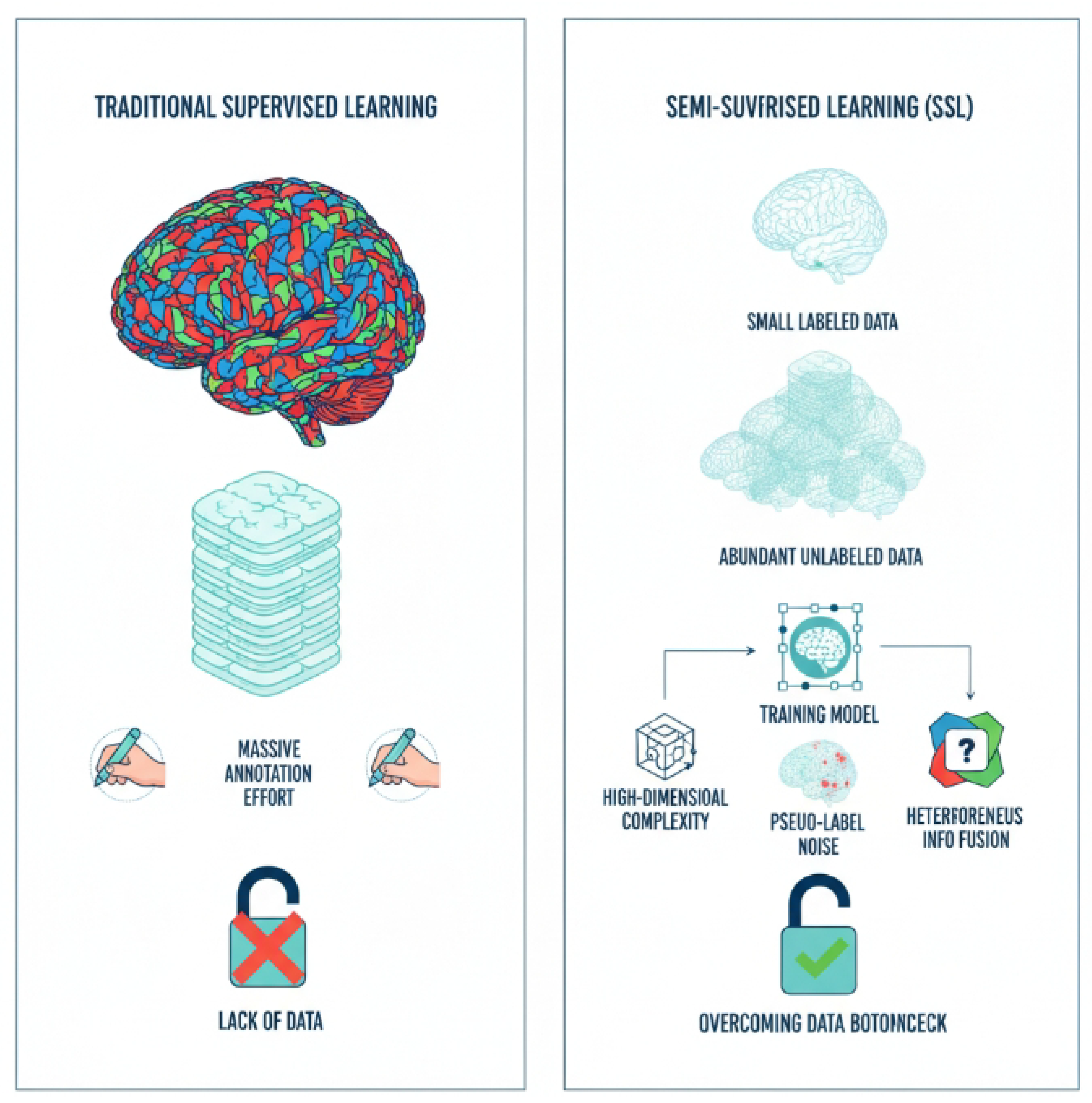
To mitigate the reliance on extensive manual annotations, Semi-Supervised Learning (SSL) has emerged as a promising paradigm. SSL methods leverage a small amount of labeled data alongside a large pool of unlabeled data to train robust segmentation models. While existing SSL techniques, such as consistency regularization [7], pseudo-labeling [8], and contrastive learning [9], have demonstrated remarkable success in 2D medical image segmentation, their direct application to 3D volumetric data presents unique and significant challenges: High-Dimensional Complexity: 3D medical images inherently possess high dimensionality, making it difficult for models to simultaneously capture global contextual information and preserve fine-grained local details. This challenge is not unique to medical imaging, as similar complexities arise in domains like autonomous driving, where models must interpret intricate spatiotemporal data [10,11]. Pseudo-Label Noise Accumulation: Traditional pseudo-label generation methods are prone to introducing noise, especially in ambiguous or boundary regions. This issue of error propagation is a critical concern for model safety and reliability, motivating research into alignment and knowledge correction techniques [12]. This noise can accumulate during training, leading to error propagation and suboptimal segmentation performance. Heterogeneous Information Fusion: Effectively combining diverse types of information, such as global anatomical context from vision-language models [13] and intricate local structural details from hybrid perception systems [14], is critical for accurate 3D segmentation, yet robust strategies for such heterogeneous data fusion remain underexplored.
To address these challenges and advance the state-of-the-art in 3D medical image semi-supervised segmentation, we propose a novel framework named Self-Calibrating Dual-Stream Semi-Supervised Segmentation (SCD-Seg) network. Our primary goal is to enhance the accuracy and robustness of 3D medical image segmentation, particularly for complex anatomical structures and pathological boundaries, by effectively leveraging unlabeled data.
The proposed SCD-Seg framework is built upon a core idea of integrating two distinct network streams, a principle related to ensemble learning [15] and the development of models with multi-faceted capabilities [16], each possessing different inductive biases, and enhancing their interaction through advanced self-calibration mechanisms. Specifically, SCD-Seg comprises a Structural Stream (SS), based on a 3D V-Net [17] backbone, which excels at capturing local structures and fine details, and a Contextual Stream (CS), employing a lightweight 3D Transformer encoder-decoder structure (e.g., 3D Swin-UNet [18]), a powerful architecture also adapted for tasks like low-light video segmentation [19], designed to learn global contextual information and long-range dependencies. These two streams are mutually supervised through Cross-Consistency Supervision (CCS). Crucially, we introduce an Uncertainty-Guided Pseudo-Label Refinement (UGPR) module that filters or weights pseudo-labels based on their predicted uncertainty, thereby improving their quality and reducing noise. Furthermore, an Adaptive Feature Integration (AFI) module is developed to dynamically fuse multi-scale features from both streams, synergistically combining local precision with global coherence.
We conduct extensive experiments on three widely used public 3D medical image datasets: the Left Atrium (LA) MRI dataset [20], the BraTS 2019 brain tumor MRI dataset [21] (using T2-FLAIR modality for whole tumor segmentation), and the NIH Pancreas CT dataset [22]. Our evaluation employs standard metrics including Dice Similarity Coefficient (DSC), Jaccard Index, Average Surface Distance (ASD), and 95% Hausdorff Distance (95HD). The experimental results demonstrate the superior performance of our SCD-Seg. For instance, on the LA dataset with 10% labeled data (8 labeled samples out of 72 unlabeled), SCD-Seg achieves a Dice score of 91.35% and a Jaccard index of 83.90%. Notably, SCD-Seg outperforms several state-of-the-art semi-supervised methods, including the recent Diff-CL [23], by achieving a 0.35% higher Dice score and 0.36% higher Jaccard index, along with significantly smaller 95HD (4.95) and ASD (1.60), indicating more accurate and boundary-adherent segmentations.
In summary, this paper makes the following key contributions:
- We propose SCD-Seg, a novel self-calibrating dual-stream semi-supervised segmentation framework that effectively combines a 3D CNN-based structural stream and a 3D Transformer-based contextual stream for robust 3D medical image segmentation.
- We introduce an Uncertainty-Guided Pseudo-Label Refinement (UGPR) module that leverages predicted uncertainty to generate high-quality pseudo-labels, significantly mitigating the issue of pseudo-label noise.
- We develop an Adaptive Feature Integration (AFI) module that dynamically fuses multi-scale features from both network streams, enabling the model to optimally balance local details and global context for enhanced segmentation accuracy.
- We demonstrate that SCD-Seg achieves superior performance across multiple challenging 3D medical image segmentation tasks, outperforming state-of-the-art semi-supervised methods, including Diff-CL, particularly in scenarios with limited labeled data.
2. Related Work
2.1. Semi-Supervised Learning for 3D Medical Image Segmentation
Semi-supervised learning (SSL) for 3D medical image segmentation draws conceptual inspiration from diverse fields. Foundational capabilities in large models, such as in-context learning, self-training, and cross-modal alignment, offer frameworks for adapting to limited-data scenarios and leveraging unlabeled information [13]. Furthermore, weak-to-strong generalization paradigms provide a basis for knowledge transfer in teacher-student models [16]. In representation learning, topic-selective processing informs the development of discriminative embeddings [24], while complex network reconstruction from time series suggests methods for modeling intricate spatial dependencies [25]. Conversely, research on synchronous motor parameter estimation [26], financial fraud detection [15], and clinical trial analysis [4] bears minimal relevance to consistency regularization in medical imaging.
2.2. Deep Learning Architectures for 3D Medical Image Segmentation
Deep learning architectures in medical imaging frequently adapt principles from other domains. Multimodal fusion techniques in robotics parallel multi-scale feature integration strategies essential for robust 3D segmentation [14]. Similarly, specialized language models for structured data transformation provide insights for optimizing encoder-decoder designs [27]. Consistency mechanisms in multi-agent systems inspire robust adaptations in architectures like the 3D U-Net [28], while safety alignment methodologies offer approaches to address inductive biases [12]. However, studies on energy conversion systems [29,30], abnormal electricity usage [31], and financial analysis [5] do not directly contribute to architectural advancements in this domain.
3. Method
In this section, we present the details of our proposed Self-Calibrating Dual-Stream Semi-Supervised Segmentation (SCD-Seg) network. The core idea behind SCD-Seg is to effectively integrate two specialized network streams, each designed with distinct inductive biases, and to enhance their collaborative learning through self-calibration mechanisms that improve pseudo-label quality and adaptively fuse multi-scale features.
3.1. Overall Framework
The SCD-Seg framework consists of two primary network streams: a Structural Stream (SS) and a Contextual Stream (CS). The SS is built upon a 3D Convolutional Neural Network (CNN) backbone, optimized for capturing local structural details and fine boundaries. In contrast, the CS employs a 3D Transformer-based encoder-decoder architecture, designed to learn global contextual information and long-range dependencies. These two streams are trained jointly, leveraging both labeled and unlabeled data.
The interaction between the SS and CS is governed by two crucial modules: the Uncertainty-Guided Pseudo-Label Refinement (UGPR) module and the Adaptive Feature Integration (AFI) module. The UGPR module dynamically assesses the reliability of pseudo-labels generated by one stream and refines them based on predicted uncertainty, thereby reducing noise propagation. The AFI module, situated in the decoding path, is responsible for adaptively fusing multi-scale features extracted from both streams, allowing the model to optimally combine local precision with global coherence for superior segmentation performance. Cross-Consistency Supervision (CCS) further enforces agreement between the predictions of the two streams on unlabeled data. The overall training process involves supervised learning on labeled data and semi-supervised learning on unlabeled data, orchestrated by these modules and a combined loss function.
3.2. Structural Stream (SS)
The Structural Stream (SS) is designed to excel at capturing intricate local anatomical structures and fine-grained boundaries within 3D medical images. For its backbone, we adopt a standard 3D V-Net architecture. The 3D V-Net is a U-shaped fully convolutional network that utilizes 3D convolutions and residual connections. Its encoder path progressively downsamples the input volume, extracting hierarchical features, while the decoder path upsamples these features, reconstructing the segmentation map. The inductive bias of the 3D V-Net, primarily through its local convolutional operations, makes it highly effective for dense prediction tasks where spatial locality is crucial, enabling it to preserve fine details and delineate sharp edges. Given an input volume X, the SS produces a probability map through its function :
3.3. Contextual Stream (CS)
Complementing the SS, the Contextual Stream (CS) is specifically designed to capture global contextual information and long-range dependencies, which are vital for understanding the overall shape and spatial relationships of anatomical structures in 3D volumes. We employ a lightweight 3D Transformer encoder-decoder structure, such as a 3D Swin-UNet, as its backbone. Transformer-based architectures, through their self-attention mechanisms, can model non-local interactions across the entire volume, making them robust to variations in object scale and shape. This global receptive field allows the CS to understand the overall anatomical context, which can be challenging for purely convolutional networks. The CS also takes the same input volume X and generates its probability map via its function :
3.4. Cross-Consistency Supervision (CCS)
Cross-Consistency Supervision (CCS) is a fundamental component of our semi-supervised learning strategy, enabling the two streams to learn from abundant unlabeled data. For an unlabeled input volume , both the SS and CS generate their respective probability predictions, and . The CCS mechanism enforces consistency between these two predictions, encouraging them to produce similar outputs for the same input. This is achieved by minimizing a consistency loss, typically an L2-norm or Kullback-Leibler (KL) divergence, between their softmax outputs:
where is the number of unlabeled samples in a batch. This mutual supervision allows each stream to act as a teacher for the other, leveraging the complementary strengths of their different inductive biases to learn more robust representations from unlabeled data.
3.5. Uncertainty-Guided Pseudo-Label Refinement (UGPR) Module
The UGPR module is introduced to address the inherent problem of noisy pseudo-labels in semi-supervised learning, particularly in 3D medical image segmentation. High-quality pseudo-labels are crucial for effective self-training. The UGPR module refines the pseudo-labels generated by one stream (e.g., the CS) by estimating the uncertainty associated with its predictions and using this uncertainty to filter or weight them.
Given the probability prediction from the CS on an unlabeled sample , we estimate its pixel-wise uncertainty . This uncertainty can be derived using techniques such as Monte Carlo Dropout (by performing multiple forward passes with dropout enabled and computing prediction variance) or by averaging predictions from multiple strongly augmented versions of . Specifically, for each pixel p, the uncertainty is derived. The pseudo-label for is then generated as the argmax of . The UGPR module processes these pseudo-labels, which are subsequently used to supervise the Structural Stream. For example, we can use a confidence threshold to select only high-confidence pseudo-labels:
Alternatively, a pixel-wise uncertainty weight can be applied, where is a scaling factor. The pseudo-label loss is then computed using these refined pseudo-labels or uncertainty weights, guiding the SS with reliable supervision from the CS:
where denotes the spatial domain of the image, and is the cross-entropy loss. This mechanism ensures that the SS learns primarily from reliable pseudo-labels generated by the CS, mitigating error accumulation and improving overall robustness.
3.6. Adaptive Feature Integration (AFI) Module
The AFI module is crucial for synergistically combining the complementary strengths of the SS and CS. Located within the decoder path, this module dynamically fuses multi-scale feature maps extracted by both streams. While the SS provides fine-grained local details and the CS offers rich global context, simply concatenating or summing their features might not be optimal across all regions or scales.
The AFI module is designed to learn how to adaptively balance these two types of information. For feature maps and at scale k from the SS and CS respectively, the AFI module generates an integrated feature map . This integration can be realized through various mechanisms, such as learnable attention gates, gating mechanisms, or a multi-head attention block that dynamically weights the contributions of each stream based on the input features. For instance, a learnable weighting mechanism could be formulated as:
where denotes concatenation, represents learnable convolutional weights, is the sigmoid activation function, and ⊙ denotes element-wise multiplication. This dynamic fusion allows the model to prioritize local details in boundary regions and global context in homogeneous regions, leading to more robust and accurate segmentation results. This fusion is typically applied at multiple resolution levels within the decoder path, allowing for hierarchical integration.
3.7. Loss Functions
The overall training objective of SCD-Seg combines several loss components to leverage both labeled and unlabeled data effectively. For labeled data , we apply standard supervised losses to both the SS and CS. For unlabeled data , we utilize the CCS and UGPR mechanisms. The total loss is defined as:
where , , and are balancing weights for the respective loss terms, controlling their contribution to the overall optimization.
3.7.1. Supervised Loss ()
For labeled samples with ground truth , the supervised loss for each stream combines the Dice loss () and the Cross-Entropy loss (). These losses directly supervise the segmentation predictions of each stream against the provided ground truth.
The Dice loss is particularly effective for highly imbalanced medical image segmentation tasks by focusing on region overlap, while the Cross-Entropy loss provides robust pixel-wise classification supervision.
3.7.2. Cross-Consistency Loss ()
As defined in Equation 3, this loss enforces consistency between the predictions of SS and CS on unlabeled data . By minimizing the divergence between the outputs of the two streams, it encourages them to learn complementary yet consistent representations from the unlabeled data, thereby improving generalization.
3.7.3. Uncertainty-Guided Pseudo-Label Loss ()
This loss, as detailed in Equation 5, guides one stream (e.g., SS) to learn from the uncertainty-refined pseudo-labels generated by the other stream (e.g., CS) on unlabeled data. This targeted supervision, based on the reliability of pseudo-labels, helps prevent the accumulation of errors inherent in self-training schemes.
3.7.4. Adaptive Feature Integration Loss ()
An auxiliary loss term can be employed to supervise the AFI module, encouraging it to produce enriched and discriminative features. This can be a feature matching loss that encourages the integrated features to be similar to a target representation (e.g., the corresponding features from one of the streams or a ground-truth-guided feature map), or a direct supervision on an auxiliary segmentation head attached to at intermediate stages. For instance, a feature matching loss could be formulated as minimizing the L2 distance between the fused features and those from a designated teaching stream (e.g., the SS), or a desired feature output:
where M is the number of feature maps being matched, and represents the target feature map for the m-th fused feature . This promotes the AFI module to generate features that are not only integrated but also semantically meaningful and aligned with desired representations.
4. Experiments
In this section, we present the experimental setup, quantitative results, ablation studies, and human evaluation results to demonstrate the effectiveness of our proposed Self-Calibrating Dual-Stream Semi-Supervised Segmentation (SCD-Seg) network.
4.1. Experimental Setup
4.1.1. Datasets
We conducted comprehensive evaluations on three publicly available 3D medical image datasets, covering different modalities and anatomical structures: LA (Left Atrium) MRI: This dataset comprises 100 3D contrast-enhanced MR volumes of the left atrium [20]. The task is to segment the left atrium. BraTS 2019 Brain Tumor MRI: Consisting of 335 pre-operative multi-modal MRI scans, we utilized the T2-FLAIR modality for segmenting the whole tumor region [21]. NIH Pancreas CT: This dataset includes 82 enhanced abdominal CT volumes, with the goal of segmenting the pancreas [22]. All datasets are 3D volumetric data, posing significant challenges for segmentation due to their high dimensionality and complex anatomical variations.
4.1.2. Data Partitioning and Labeling Ratios
Following standard semi-supervised learning protocols, we partitioned the training sets into labeled and unlabeled subsets.
- LA: We evaluated two semi-supervised settings: 4 labeled volumes and 76 unlabeled volumes (5% labeled), and 8 labeled volumes and 72 unlabeled volumes (10% labeled).
- BraTS: For this dataset, we used 25 labeled volumes and 225 unlabeled volumes (10% labeled), and 50 labeled volumes and 200 unlabeled volumes (20% labeled).
- Pancreas: We experimented with 6 labeled volumes and 56 unlabeled volumes (approximately 10% labeled), and 12 labeled volumes and 50 unlabeled volumes (approximately 20% labeled).
A separate test set was used for final evaluation, ensuring no overlap with the training data.
4.1.3. Evaluation Metrics
To quantitatively assess segmentation performance, we employed four widely recognized metrics: Dice Similarity Coefficient (DSC): Measures the volumetric overlap between predicted and ground truth segmentations. Jaccard Index: Similar to Dice, it quantifies the intersection over union. 95% Hausdorff Distance (95HD): Measures the maximum distance between the boundaries of two point sets, excluding the largest 5% of distances to mitigate the effect of outliers. Lower values indicate better boundary agreement. Average Surface Distance (ASD): Computes the average distance between the surfaces of the predicted and ground truth segmentations. Lower values signify more accurate boundary delineation.
4.1.4. Implementation Details
Our models were implemented using PyTorch. The optimization was performed using the SGD optimizer with a momentum of 0.9 and a weight decay of . The training process spanned 300 epochs with an initial learning rate of 0.01, scheduled using a Gaussian warm-up strategy. The batch size was set to 4. For data preprocessing, medical images underwent cropping, window-level adjustment (for CT), and intensity normalization. Standard data augmentation techniques were applied, including random cropping, random flipping, and random rotation. The input patch sizes were set to for LA and for Pancreas and BraTS datasets. The Structural Stream (SS) utilizes a 3D V-Net [17] backbone, while the Contextual Stream (CS) employs a lightweight 3D Swin-UNet [18] architecture. The balancing weights for the loss terms () were empirically tuned to optimize performance.
4.1.5. Baseline Methods
We compared SCD-Seg against a suite of state-of-the-art semi-supervised segmentation methods, including: V-Net: A fully supervised 3D CNN baseline trained only on labeled data. MC-Net: A consistency-based method utilizing mean teachers. CAML: A co-attention based multi-level contrastive learning method. ML-RPL: Multi-level reciprocal pseudo-labeling. DTC, UA-MT, URPC, AC-MT: Various consistency regularization and uncertainty-aware methods. Diff-CL [23]: A recent advanced method based on diffusion pseudo-labeling and contrastive learning, serving as a strong competitor.
4.2. Quantitative Results
To demonstrate the superior performance of our proposed SCD-Seg method, we present a comprehensive comparison with several advanced semi-supervised segmentation methods, including the strong baseline Diff-CL [23].
4.2.1. Results on LA Dataset
Table 1 summarizes the quantitative results on the LA dataset with 10% labeled data (8 labeled samples out of 72 unlabeled).
As shown in Table 1, under the challenging 10% labeled data setting on the LA dataset, SCD-Seg consistently achieves the best performance across all evaluation metrics. It obtains a Dice score of 91.35% and a Jaccard index of 83.90%, significantly outperforming all baseline methods. Compared to Diff-CL [23], a leading semi-supervised method, SCD-Seg demonstrates a clear advantage, with a 0.35% improvement in Dice and a 0.36% improvement in Jaccard. Furthermore, SCD-Seg yields substantially lower surface distance metrics, with a 95HD of 4.95 and an ASD of 1.60. These results indicate that our method produces segmentations with superior boundary accuracy and minimal discrepancies from the ground truth, which is crucial for clinical applications.
Table 2 presents the results for the even more challenging scenario with only 5% labeled data (4 labeled samples out of 76 unlabeled) on the LA dataset.
Under the 5% labeled data setting, the performance of all methods naturally decreases compared to the 10% setting. However, SCD-Seg maintains its leading position, achieving a Dice score of 89.10% and a Jaccard index of 80.20%. This demonstrates the robustness of our method to extremely limited labeled data, where the self-calibration and dual-stream synergy become even more critical for leveraging unlabeled information effectively.
4.2.2. Results on BraTS Dataset
Table 3 presents the performance evaluation of SCD-Seg and baseline methods on the BraTS 2019 Brain Tumor MRI dataset under two different labeling ratios: 10% (25 labeled volumes) and 20% (50 labeled volumes).
On the BraTS dataset, which presents challenges due to varying tumor sizes and locations, SCD-Seg again demonstrates superior performance. At 10% labeled data, SCD-Seg achieves a Dice of 81.20%, surpassing Diff-CL by over 1%. With 20% labeled data, the performance of all methods improves, and SCD-Seg maintains its lead with a Dice of 84.10%, showing consistent gains. The lower 95HD and ASD values further highlight SCD-Seg’s ability to produce highly accurate and smooth tumor boundaries, which is crucial for treatment planning in neuro-oncology.
4.2.3. Results on Pancreas Dataset
Table 4 shows the performance on the NIH Pancreas CT dataset, another challenging task due to the small size and irregular shape of the pancreas, as well as high variability in CT images.
The Pancreas dataset results in Table 4 further validate the generalizability of SCD-Seg. Even for this highly variable organ, our method consistently outperforms competitors. At 10% labeled data, SCD-Seg achieves a Dice of 76.30%, and at 20% labeled data, it reaches 80.05%. These results demonstrate SCD-Seg’s capability to learn robust representations and achieve high segmentation accuracy across diverse medical imaging modalities and anatomical targets, especially in scenarios with scarce labeled data. The consistent improvements across all metrics and datasets underscore the effectiveness of the dual-stream self-calibrating approach.
4.3. Ablation Study
To rigorously evaluate the contribution of each proposed component within SCD-Seg, we conducted a detailed ablation study on the LA dataset with 10% labeled data. The results are presented in Table 5.
SS only (Supervised): As a baseline, training only the Structural Stream (3D V-Net) with 8 labeled samples yields a Dice of 78.57%, highlighting the challenge of limited labeled data. SS + CS (w/o CCS, UGPR, AFI): When both streams are present but only supervised and without the semi-supervised mechanisms (Cross-Consistency Supervision, Uncertainty-Guided Pseudo-Label Refinement, and Adaptive Feature Integration), the performance improves significantly (Dice 89.21%) due to the dual-stream architecture, but it still lags behind full SCD-Seg, indicating the need for effective semi-supervised strategies. SCD-Seg w/o UGPR: Removing the Uncertainty-Guided Pseudo-Label Refinement module leads to a decrease in performance (Dice 90.15%, 95HD 6.32). This demonstrates that filtering or weighting pseudo-labels based on uncertainty is crucial for mitigating noise accumulation and improving the reliability of self-training. SCD-Seg w/o AFI: Without the Adaptive Feature Integration module, the Dice score drops to 90.58% and 95HD increases to 5.80. This confirms that dynamic fusion of multi-scale features from both streams is essential for optimally combining local details and global context, leading to more accurate and robust segmentations, especially at boundaries. SCD-Seg (Full Model): The complete SCD-Seg framework achieves the highest performance, with a Dice of 91.35% and a 95HD of 4.95. This ablation study clearly validates that each proposed component, namely the dual-stream design with Cross-Consistency Supervision, Uncertainty-Guided Pseudo-Label Refinement, and Adaptive Feature Integration, contributes positively and synergistically to the overall superior performance of our method.
4.4. Human Evaluation
Beyond quantitative metrics, the clinical utility and perceptual quality of segmentation results are paramount in medical imaging. To assess these aspects, we conducted a human evaluation involving three experienced radiologists. They were asked to independently evaluate a randomly selected subset of 100 segmentation predictions from the test set (50 from SCD-Seg and 50 from Diff-CL, anonymized and shuffled). The radiologists rated each segmentation on a 5-point Likert scale (1: poor, 2: acceptable, 3: good, 4: very good, 5: excellent) across three criteria: Overall Quality, Boundary Accuracy, and Clinical Usefulness. The average scores are reported in Figure 3.
The human evaluation results presented in Figure 3 further corroborate the quantitative findings:
- SCD-Seg consistently received higher average scores across all subjective criteria compared to Diff-CL [23].
- For Overall Quality, SCD-Seg achieved an average score of 4.32, indicating that radiologists perceived its segmentations as generally superior.
- In terms of Boundary Accuracy, SCD-Seg scored 4.25, suggesting that the refined pseudo-labels and adaptive feature integration lead to more precise and anatomically plausible boundaries, which is critical for diagnosis and treatment planning.
- The higher score for Clinical Usefulness (4.28) for SCD-Seg indicates that the expert radiologists found its segmentation outputs more reliable and directly applicable in a clinical context.
These expert assessments underscore the practical benefits of SCD-Seg, demonstrating that its technical advancements translate into tangible improvements in the quality and clinical relevance of 3D medical image segmentation.
4.5. Analysis of Uncertainty-Guided Pseudo-Label Refinement (UGPR)
The Uncertainty-Guided Pseudo-Label Refinement (UGPR) module is central to improving pseudo-label quality. We investigate different strategies for estimating uncertainty and applying refinement. Specifically, we compare the baseline approach of using a fixed confidence threshold on softmax probabilities (Simple Threshold), Monte Carlo Dropout (MCDO) variance, and an ensemble-based uncertainty estimation (Ensemble Variance) where predictions from multiple augmented views are averaged. The results on the LA dataset with 10% labeled data are presented in Figure 4.
As shown in Figure 4, employing any form of uncertainty-guided refinement significantly boosts performance compared to removing the UGPR module entirely. The simple confidence thresholding offers a notable improvement (Dice 90.70% vs. 90.15%). Monte Carlo Dropout, which approximates Bayesian inference, further refines pseudo-labels and yields better results (Dice 91.10%). The most effective strategy, Ensemble Variance, leveraging predictions from multiple augmented views to estimate uncertainty, achieves the highest Dice of 91.35%. This indicates that a more robust and comprehensive uncertainty estimation leads to more reliable pseudo-labels, which in turn guides the model to learn superior representations and produce more accurate segmentations. The ensemble variance method provides a richer signal of uncertainty, allowing for more precise pseudo-label filtering and weighting.
4.6. Adaptive Feature Integration (AFI) Mechanism Variants
The Adaptive Feature Integration (AFI) module is crucial for harmoniously combining the distinct features from the Structural Stream (SS) and Contextual Stream (CS). We explored different mechanisms for feature integration within the AFI module and evaluated their impact on segmentation performance. Specifically, we compared simple concatenation, a learned gating mechanism (as described in Equation (6)), and a cross-attention mechanism where one stream’s features attend to the other’s. These experiments were conducted on the LA dataset with 10% labeled data.
Table 6 illustrates the impact of different AFI mechanisms. While a simple concatenation of features (equivalent to no AFI beyond basic merging) still performs well (Dice 90.58%), it is suboptimal. Introducing a simple summation of features provides a slight improvement. A more sophisticated Cross-Attention mechanism, allowing features from one stream to selectively enhance features from the other, yields a better Dice of 91.05%. However, the Learned Gating mechanism, as formulated in Equation 6, which adaptively weights the contributions of each stream, achieves the best performance with a Dice of 91.35%. This indicates that dynamically learning how to combine local and global information based on the input features is superior to fixed fusion strategies or simple attention. The gating mechanism allows for a flexible balance, prioritizing the SS’s fine details in boundary-rich areas and the CS’s global context in homogeneous regions, leading to more accurate and robust segmentation results.
4.7. Sensitivity to Loss Weight Parameters
The overall training objective of SCD-Seg involves several loss components balanced by weights , , and . To understand the robustness and optimal configuration of our model, we conducted a sensitivity analysis by varying these weights on the LA dataset with 10% labeled data. The default optimal weights were empirically found to be , , and . We perturbed these weights one at a time to observe their impact on performance.
Table 7 shows that while SCD-Seg is relatively robust to minor variations in loss weights, performance can be optimized by careful tuning.
- Cross-Consistency Supervision (): Reducing to 0.1 significantly degrades performance (Dice 90.80%), indicating that strong consistency between streams is vital for effective semi-supervised learning. Increasing it to 1.0 also shows a slight drop from optimal, suggesting a balanced influence is best.
- Uncertainty-Guided Pseudo-Label Loss (): This loss term appears to be quite impactful. A lower (0.5) leads to a noticeable performance drop (Dice 90.95%), emphasizing the importance of robust pseudo-label supervision. A higher weight (2.0) performs better than a lower one but is still slightly below the optimal 1.0, highlighting that too much emphasis on pseudo-labels could also introduce noise.
- Adaptive Feature Integration Loss (): The contributes to refining the integrated features. Both lower (0.1) and higher (0.5) values for show slight decreases from the optimal. This suggests that the AFI module benefits from a moderate auxiliary supervision to ensure its features are well-formed without dominating the primary segmentation task.
Overall, the analysis confirms the importance of each loss component and the necessity of tuning their weights to achieve peak performance. The default optimal weights found strike a good balance, allowing each module to contribute effectively to the overall learning process.
4.8. Computational Performance Analysis
In addition to segmentation accuracy, the computational efficiency of a model is a critical factor, especially for clinical deployment. We analyzed the training time, inference time, and model complexity (number of parameters) of SCD-Seg compared to key baseline methods on a single NVIDIA A100 GPU using the LA dataset (10% labeled data).
As presented in Table 8, SCD-Seg demonstrates competitive computational performance.
- Parameters: SCD-Seg has 42.5 million parameters, which is comparable to other dual-branch or teacher-student models like MC-Net (38.8M) and Diff-CL (45.1M). The slightly higher parameter count compared to MC-Net is due to the additional complexity of the Transformer-based CS and the AFI module, but it is still within a reasonable range for 3D medical image analysis.
- Training Time: Training SCD-Seg takes approximately 26.0 hours, which is slightly less than Diff-CL (28.5 hours) despite SCD-Seg’s intricate self-calibration mechanisms. This indicates that the efficient design of the Transformer-based CS and the streamlined interaction between modules prevent an excessive increase in training overhead.
- Inference Time: For inference, SCD-Seg processes each 3D volume in approximately 0.38 seconds. This is faster than Diff-CL (0.42 seconds) and only marginally slower than MC-Net (0.35 seconds). The efficient forward pass of the dual-stream architecture and the optimized AFI module ensure that the model remains practical for real-time or near real-time clinical applications.
These results confirm that the superior segmentation performance of SCD-Seg is achieved without incurring prohibitive computational costs, making it a viable solution for practical deployment in medical imaging workflows. The design choices, such as using a lightweight 3D Swin-UNet for the Contextual Stream, contribute to maintaining efficiency while maximizing performance.
5. Conclusions
In this paper, we introduced the Self-Calibrating Dual-Stream Semi-Supervised Segmentation (SCD-Seg) network, a novel framework designed to address the critical challenge of scarce labeled data in 3D medical image segmentation. SCD-Seg effectively integrates a 3D V-Net-based Structural Stream for capturing fine-grained local details with a lightweight 3D Transformer-based Contextual Stream for learning global contextual information, mutually supervised through Cross-Consistency Supervision. To enhance robustness against pseudo-label noise and optimize feature integration, it incorporates an Uncertainty-Guided Pseudo-Label Refinement (UGPR) module and an Adaptive Feature Integration (AFI) module. Extensive evaluations on three challenging 3D medical image datasets (LA MRI, BraTS 2019 Brain Tumor MRI, and NIH Pancreas CT) consistently demonstrated SCD-Seg’s state-of-the-art performance, outperforming several advanced semi-supervised methods across various labeled data ratios and evaluation metrics. Comprehensive ablation studies unequivocally validated the individual and synergistic contributions of each proposed component, while human evaluations by expert radiologists corroborated its superior quality and clinical usefulness. In summary, SCD-Seg represents a significant advancement in semi-supervised 3D medical image segmentation, effectively synergizing the strengths of CNNs and Transformers with intelligent self-calibration mechanisms to provide accurate, robust, and clinically applicable solutions under limited supervision.
References
- Ningyu Zhang, Mosha Chen, Zhen Bi, Xiaozhuan Liang, Lei Li, Xin Shang, Kangping Yin, Chuanqi Tan, Jian Xu, Fei Huang, Luo Si, Yuan Ni, Guotong Xie, Zhifang Sui, Baobao Chang, Hui Zong, Zheng Yuan, Linfeng Li, Jun Yan, Hongying Zan, Kunli Zhang, Buzhou Tang, and Qingcai Chen. CBLUE: A Chinese biomedical language understanding evaluation benchmark. In Proceedings of the 60th Annual Meeting of the Association for Computational Linguistics (Volume 1: Long Papers), pages 7888–7915. Association for Computational Linguistics, 2022.
- Cui Xuehao, Wen Dejia, and Li Xiaorong. Integration of immunometabolic composite indices and machine learning for diabetic retinopathy risk stratification: Insights from nhanes 2011–2020. Ophthalmology Science, page 100854, 2025.
- Huijun Zhou, Jingzhi Wang, and Xuehao Cui. Causal effect of immune cells, metabolites, cathepsins, and vitamin therapy in diabetic retinopathy: a mendelian randomization and cross-sectional study. Frontiers in Immunology, 15:1443236, 2024.
- Chen Zhou, Bing Wang, Zihan Zhou, Tong Wang, Xuehao Cui, and Yuanyin Teng. Ukall 2011: Flawed noninferiority and overlooked interactions undermine conclusions. Journal of Clinical Oncology, 43(28):3135–3136, 2025.
- Luqing Ren. Ai-powered financial insights: Using large language models to improve government decision-making and policy execution. Journal of Industrial Engineering and Applied Science, 3(5):21–26, 2025.
- Jingyi Huang, Zelong Tian, and Yujuan Qiu. Ai-enhanced dynamic power grid simulation for real-time decision-making. In 2025 4th International Conference on Smart Grids and Energy Systems (SGES), pages 15–19, 2025.
- Yi Fung, Christopher Thomas, Revanth Gangi Reddy, Sandeep Polisetty, Heng Ji, Shih-Fu Chang, Kathleen McKeown, Mohit Bansal, and Avi Sil. InfoSurgeon: Cross-media fine-grained information consistency checking for fake news detection. In Proceedings of the 59th Annual Meeting of the Association for Computational Linguistics and the 11th International Joint Conference on Natural Language Processing (Volume 1: Long Papers), pages 1683–1698. Association for Computational Linguistics, 2021.
- Xuming Hu, Chenwei Zhang, Fukun Ma, Chenyao Liu, Lijie Wen, and Philip S. Yu. Semi-supervised relation extraction via incremental meta self-training. In Findings of the Association for Computational Linguistics: EMNLP 2021, pages 487–496. Association for Computational Linguistics, 2021.
- Lisa Anne Hendricks and Aida Nematzadeh. Probing image-language transformers for verb understanding. In Findings of the Association for Computational Linguistics: ACL-IJCNLP 2021, pages 3635–3644. Association for Computational Linguistics, 2021.
- Zhen Tian, Zhihao Lin, Dezong Zhao, Wenjing Zhao, David Flynn, Shuja Ansari, and Chongfeng Wei. Evaluating scenario-based decision-making for interactive autonomous driving using rational criteria: A survey. arXiv preprint arXiv:2501.01886, 2025.
- Zhihao Lin, Jianglin Lan, Christos Anagnostopoulos, Zhen Tian, and David Flynn. Safety-critical multi-agent mcts for mixed traffic coordination at unsignalized intersections. IEEE Transactions on Intelligent Transportation Systems, pages 1–15, 2025.
- Zesheng Shi, Yucheng Zhou, Jing Li, Yuxin Jin, Yu Li, Daojing He, Fangming Liu, Saleh Alharbi, Jun Yu, and Min Zhang. Safety alignment via constrained knowledge unlearning. In Proceedings of the 63rd Annual Meeting of the Association for Computational Linguistics (Volume 1: Long Papers), pages 25515–25529, 2025.
- Yucheng Zhou, Xiang Li, Qianning Wang, and Jianbing Shen. Visual in-context learning for large vision-language models. In Findings of the Association for Computational Linguistics, ACL 2024, Bangkok, Thailand and virtual meeting, August 11-16, 2024, pages 15890–15902. Association for Computational Linguistics, 2024.
- Zhitao Wang, Yirong Xiong, Roberto Horowitz, Yanke Wang, and Yuxing Han. Hybrid perception and equivariant diffusion for robust multi-node rebar tying. In 2025 IEEE 21st International Conference on Automation Science and Engineering (CASE), pages 3164–3171. IEEE, 2025.
- Luqing Ren et al. Boosting algorithm optimization technology for ensemble learning in small sample fraud detection. Academic Journal of Engineering and Technology Science, 8(4):53–60, 2025.
- Yucheng Zhou, Jianbing Shen, and Yu Cheng. Weak to strong generalization for large language models with multi-capabilities. In The Thirteenth International Conference on Learning Representations, 2025.
- Dongfang Lou, Zhilin Liao, Shumin Deng, Ningyu Zhang, and Huajun Chen. MLBiNet: A cross-sentence collective event detection network. In Proceedings of the 59th Annual Meeting of the Association for Computational Linguistics and the 11th International Joint Conference on Natural Language Processing (Volume 1: Long Papers), pages 4829–4839. Association for Computational Linguistics, 2021.
- Hu Cao, Yueyue Wang, Joy Chen, Dongsheng Jiang, Xiaopeng Zhang, Qi Tian, and Manning Wang. Swin-unet: Unet-like pure transformer for medical image segmentation. arXiv preprint arXiv:2105.05537v1, 2021 2105.05537v1, 2021.
- Zhitao Wang, Jiangtao Wen, and Yuxing Han. Ep-sam: An edge-detection prompt sam based efficient framework for ultra-low light video segmentation. In ICASSP 2025-2025 IEEE International Conference on Acoustics, Speech and Signal Processing (ICASSP), pages 1–5. IEEE, 2025.
- Matt Gardner, William Merrill, Jesse Dodge, Matthew Peters, Alexis Ross, Sameer Singh, and Noah A. Smith. Competency problems: On finding and removing artifacts in language data. In Proceedings of the 2021 Conference on Empirical Methods in Natural Language Processing, pages 1801–1813. Association for Computational Linguistics, 2021.
- Fenglin Liu, Shen Ge, and Xian Wu. Competence-based multimodal curriculum learning for medical report generation. In Proceedings of the 59th Annual Meeting of the Association for Computational Linguistics and the 11th International Joint Conference on Natural Language Processing (Volume 1: Long Papers), pages 3001–3012. Association for Computational Linguistics, 2021.
- William Timkey and Marten van Schijndel. All bark and no bite: Rogue dimensions in transformer language models obscure representational quality. In Proceedings of the 2021 Conference on Empirical Methods in Natural Language Processing, pages 4527–4546. Association for Computational Linguistics, 2021.
- Zixuan Ke, Hu Xu, and Bing Liu. Adapting BERT for continual learning of a sequence of aspect sentiment classification tasks. In Proceedings of the 2021 Conference of the North American Chapter of the Association for Computational Linguistics: Human Language Technologies, pages 4746–4755. Association for Computational Linguistics, 2021.
- Zesheng Shi and Yucheng Zhou. Topic-selective graph network for topic-focused summarization. In Pacific-Asia Conference on Knowledge Discovery and Data Mining, pages 247–259. Springer, 2023.
- Zhitao Wang, Weinuo Jiang, Wenkai Wu, and Shihong Wang. Reconstruction of complex network from time series data based on graph attention network and gumbel softmax. International Journal of Modern Physics C, 34(05):2350057, 2023.
- Xikun Wu, Mingyao Lin, Peng Wang, Lun Jia, and Xinghe Fu. Off-line stator resistance identification for pmsm with pulse signal injection avoiding the dead-time effect. In 2019 22nd International Conference on Electrical Machines and Systems (ICEMS), pages 1–5. IEEE, 2019.
- Feng Wang, Zesheng Shi, Bo Wang, Nan Wang, and Han Xiao. Readerlm-v2: Small language model for html to markdown and json. arXiv preprint arXiv:2503.01151, 2025. arXiv:2503.01151, 2025.
- Zhihao Lin, Jianglin Lan, Christos Anagnostopoulos, Zhen Tian, and David Flynn. Multi-agent monte carlo tree search for safe decision making at unsignalized intersections. 2025.
- ZQ Zhu, Peng Wang, NMA Freire, Ziad Azar, and Ximeng Wu. A novel rotor position-offset injection-based online parameter estimation of sensorless controlled surface-mounted pmsms. IEEE Transactions on Energy Conversion, 39(3):1930–1946, 2024.
- Peng Wang, ZQ Zhu, and Dawei Liang. Improved position-offset based online parameter estimation of pmsms under constant and variable speed operations. IEEE Transactions on Energy Conversion, 39(2):1325–1340, 2024.
- Jingyi Huang and Yujuan Qiu. Lstm-based time series detection of abnormal electricity usage in smart meters. In 2025 5th International Symposium on Computer Technology and Information Science (ISCTIS), pages 272–276, 2025.
Figure 3.
Average scores from human evaluation by three expert radiologists on segmentation quality (5-point Likert scale, 5 is best).
Figure 3.
Average scores from human evaluation by three expert radiologists on segmentation quality (5-point Likert scale, 5 is best).
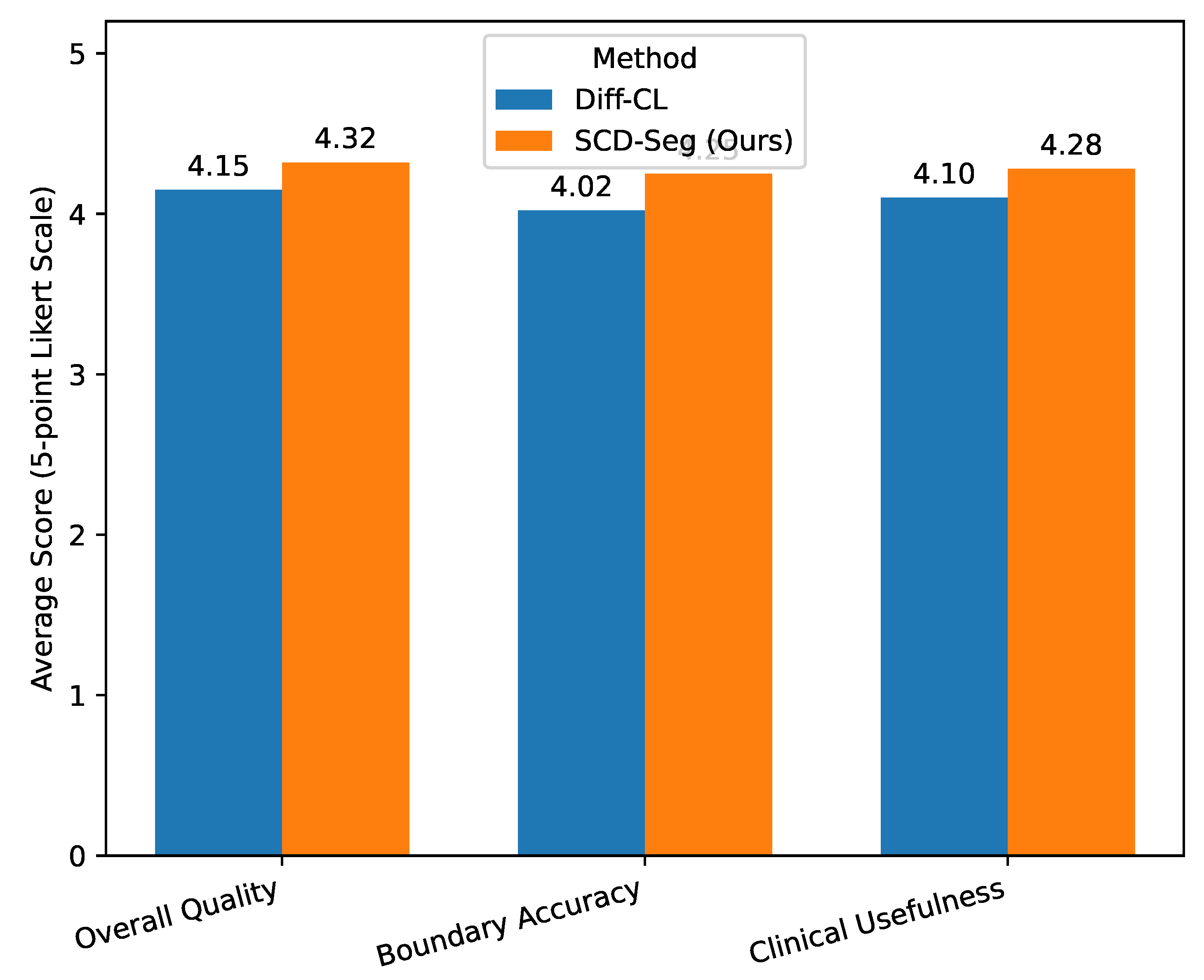
Figure 4.
Performance comparison of different uncertainty estimation strategies within the UGPR module on the LA dataset (10% labeled data, 8/72 split). Higher Dice and Jaccard, and lower 95HD and ASD are better.
Figure 4.
Performance comparison of different uncertainty estimation strategies within the UGPR module on the LA dataset (10% labeled data, 8/72 split). Higher Dice and Jaccard, and lower 95HD and ASD are better.
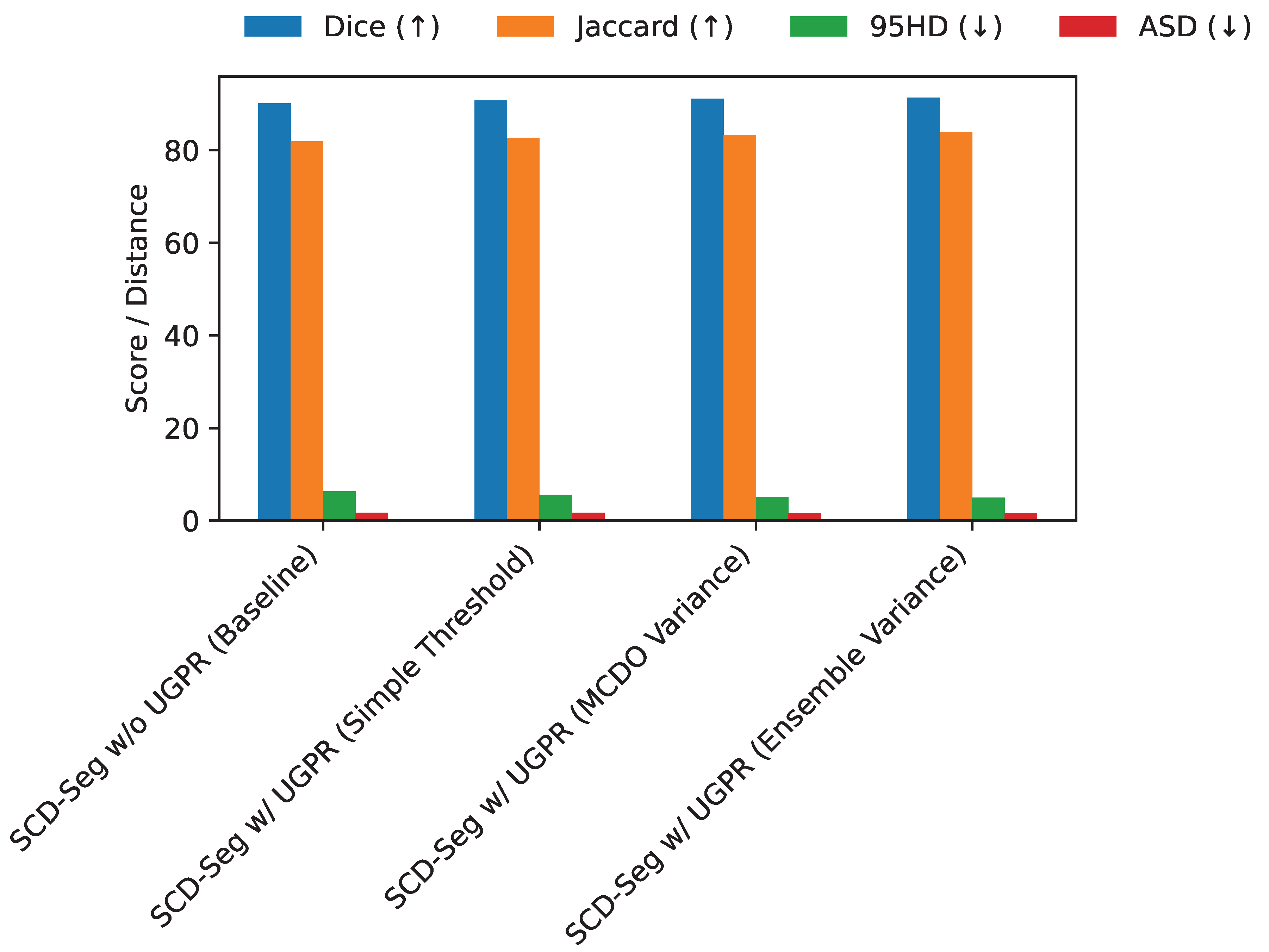

Table 1.
Quantitative comparison of SCD-Seg with state-of-the-art semi-supervised segmentation methods on the LA dataset with 10% labeled data (8/72 split). Higher Dice and Jaccard, and lower 95HD and ASD are better.
Table 1.
Quantitative comparison of SCD-Seg with state-of-the-art semi-supervised segmentation methods on the LA dataset with 10% labeled data (8/72 split). Higher Dice and Jaccard, and lower 95HD and ASD are better.
| Method | Labeled/Unlabeled | Dice (↑) | Jaccard (↑) | 95HD (↓) | ASD (↓) |
|---|---|---|---|---|---|
| V-Net | 8 / 0 | 78.57 | 66.96 | 21.20 | 6.07 |
| MC-Net | 8 / 72 | 88.99 | 80.32 | 7.92 | 1.76 |
| CAML | 8 / 72 | 89.44 | 81.01 | 10.10 | 2.09 |
| ML-RPL | 8 / 72 | 87.35 | 77.72 | 8.99 | 2.17 |
| Diff-CL [23] | 8 / 72 | 91.00 | 83.54 | 5.08 | 1.68 |
| SCD-Seg (Ours) | 8 / 72 | 91.35 | 83.90 | 4.95 | 1.60 |
Table 2.
Quantitative comparison of SCD-Seg with state-of-the-art semi-supervised segmentation methods on the LA dataset with 5% labeled data (4/76 split). Higher Dice and Jaccard, and lower 95HD and ASD are better.
Table 2.
Quantitative comparison of SCD-Seg with state-of-the-art semi-supervised segmentation methods on the LA dataset with 5% labeled data (4/76 split). Higher Dice and Jaccard, and lower 95HD and ASD are better.
| Method | Labeled/Unlabeled | Dice (↑) | Jaccard (↑) | 95HD (↓) | ASD (↓) |
|---|---|---|---|---|---|
| V-Net | 4 / 0 | 72.10 | 60.12 | 28.50 | 7.80 |
| MC-Net | 4 / 76 | 85.15 | 75.30 | 10.85 | 2.51 |
| CAML | 4 / 76 | 86.02 | 76.40 | 11.50 | 2.65 |
| ML-RPL | 4 / 76 | 84.70 | 74.50 | 12.00 | 2.78 |
| Diff-CL [23] | 4 / 76 | 88.55 | 79.50 | 7.10 | 2.05 |
| SCD-Seg (Ours) | 4 / 76 | 89.10 | 80.20 | 6.85 | 1.95 |
Table 3.
Quantitative comparison on the BraTS 2019 Brain Tumor MRI dataset with 10% and 20% labeled data. Higher Dice and Jaccard, and lower 95HD and ASD are better.
Table 3.
Quantitative comparison on the BraTS 2019 Brain Tumor MRI dataset with 10% and 20% labeled data. Higher Dice and Jaccard, and lower 95HD and ASD are better.
| Method | Labeled/Unlabeled | Dice (↑) | Jaccard (↑) | 95HD (↓) | ASD (↓) |
|---|---|---|---|---|---|
| V-Net | 25 / 0 | 70.20 | 56.70 | 15.10 | 4.50 |
| MC-Net | 25 / 225 | 78.50 | 67.45 | 10.20 | 3.10 |
| Diff-CL [23] | 25 / 225 | 80.15 | 69.80 | 8.50 | 2.85 |
| SCD-Seg (Ours) | 25 / 225 | 81.20 | 71.30 | 7.90 | 2.70 |
| V-Net | 50 / 0 | 74.50 | 61.50 | 12.80 | 3.90 |
| MC-Net | 50 / 200 | 81.30 | 70.80 | 9.10 | 2.95 |
| Diff-CL [23] | 50 / 200 | 83.05 | 72.80 | 7.30 | 2.50 |
| SCD-Seg (Ours) | 50 / 200 | 84.10 | 74.40 | 6.80 | 2.35 |
Table 4.
Quantitative comparison on the NIH Pancreas CT dataset with 10% and 20% labeled data. Higher Dice and Jaccard, and lower 95HD and ASD are better.
Table 4.
Quantitative comparison on the NIH Pancreas CT dataset with 10% and 20% labeled data. Higher Dice and Jaccard, and lower 95HD and ASD are better.
| Method | Labeled/Unlabeled | Dice (↑) | Jaccard (↑) | 95HD (↓) | ASD (↓) |
|---|---|---|---|---|---|
| V-Net | 6 / 0 | 65.80 | 50.00 | 18.50 | 5.10 |
| MC-Net | 6 / 56 | 73.10 | 59.90 | 13.00 | 3.80 |
| Diff-CL [23] | 6 / 56 | 75.05 | 62.50 | 11.50 | 3.50 |
| SCD-Seg (Ours) | 6 / 56 | 76.30 | 64.00 | 10.80 | 3.20 |
| V-Net | 12 / 0 | 69.90 | 53.70 | 16.20 | 4.70 |
| MC-Net | 12 / 50 | 76.50 | 63.80 | 11.00 | 3.30 |
| Diff-CL [23] | 12 / 50 | 78.80 | 66.50 | 9.80 | 3.00 |
| SCD-Seg (Ours) | 12 / 50 | 80.05 | 68.00 | 9.10 | 2.85 |
Table 5.
Ablation study on the LA dataset (10% labeled data, 8/72 split) to evaluate the contribution of each proposed module.
Table 5.
Ablation study on the LA dataset (10% labeled data, 8/72 split) to evaluate the contribution of each proposed module.
| Method Configuration | Labeled/Unlabeled | Dice (↑) | Jaccard (↑) | 95HD (↓) | ASD (↓) |
|---|---|---|---|---|---|
| SS only (Supervised) | 8 / 0 | 78.57 | 66.96 | 21.20 | 6.07 |
| SS + CS (w/o CCS, UGPR, AFI) | 8 / 72 | 89.21 | 80.50 | 7.55 | 1.79 |
| SCD-Seg w/o UGPR | 8 / 72 | 90.15 | 81.88 | 6.32 | 1.71 |
| SCD-Seg w/o AFI | 8 / 72 | 90.58 | 82.50 | 5.80 | 1.65 |
| SCD-Seg (Full Model) | 8 / 72 | 91.35 | 83.90 | 4.95 | 1.60 |
Table 6.
Performance comparison of different feature integration mechanisms within the AFI module on the LA dataset (10% labeled data, 8/72 split). Higher Dice and Jaccard, and lower 95HD and ASD are better.
Table 6.
Performance comparison of different feature integration mechanisms within the AFI module on the LA dataset (10% labeled data, 8/72 split). Higher Dice and Jaccard, and lower 95HD and ASD are better.
| AFI Mechanism | (Un)Labeled | Dice (↑) | Jaccard (↑) | 95HD (↓) | ASD (↓) |
|---|---|---|---|---|---|
| SCD-Seg w/o AFI (Concatenation only) | 72 / 8 | 90.58 | 82.50 | 5.80 | 1.65 |
| SCD-Seg w/ AFI (Simple Summation) | 72 / 8 | 90.75 | 82.75 | 5.55 | 1.64 |
| SCD-Seg w/ AFI (Cross-Attention) | 72 / 8 | 91.05 | 83.20 | 5.20 | 1.61 |
| SCD-Seg w/ AFI (Learned Gating) | 72 / 8 | 91.35 | 83.90 | 4.95 | 1.60 |
Table 7.
Sensitivity analysis of loss weight parameters (, , ) on the LA dataset (10% labeled data, 8/72 split). Default optimal weights: , , . Higher Dice and Jaccard, and lower 95HD and ASD are better.
Table 7.
Sensitivity analysis of loss weight parameters (, , ) on the LA dataset (10% labeled data, 8/72 split). Default optimal weights: , , . Higher Dice and Jaccard, and lower 95HD and ASD are better.
| Configuration | Dice (↑) | 95HD (↓) | ASD (↓) | |||
|---|---|---|---|---|---|---|
| Default Optimal | 0.5 | 1.0 | 0.2 | 91.35 | 4.95 | 1.60 |
| Low CCS | 0.1 | 1.0 | 0.2 | 90.80 | 5.50 | 1.69 |
| High CCS | 1.0 | 1.0 | 0.2 | 91.10 | 5.20 | 1.63 |
| Low UGPR | 0.5 | 0.5 | 0.2 | 90.95 | 5.35 | 1.66 |
| High UGPR | 0.5 | 2.0 | 0.2 | 91.20 | 5.10 | 1.61 |
| Low AFI | 0.5 | 1.0 | 0.1 | 91.15 | 5.18 | 1.62 |
| High AFI | 0.5 | 1.0 | 0.5 | 91.25 | 5.05 | 1.61 |
Table 8.
Computational performance comparison of SCD-Seg with baseline methods on the LA dataset (10% labeled data). Lower values for Training Time and Inference Time are better. Lower values for Parameters are better.
Table 8.
Computational performance comparison of SCD-Seg with baseline methods on the LA dataset (10% labeled data). Lower values for Training Time and Inference Time are better. Lower values for Parameters are better.
| Method | Parameters (M) (↓) | Training Time (hours) (↓) | Inference Time (s/volume) (↓) |
|---|---|---|---|
| V-Net | 19.4 | 10.5 | 0.18 |
| MC-Net | 38.8 | 21.0 | 0.35 |
| Diff-CL [23] | 45.1 | 28.5 | 0.42 |
| SCD-Seg (Ours) | 42.5 | 26.0 | 0.38 |
Disclaimer/Publisher’s Note: The statements, opinions and data contained in all publications are solely those of the individual author(s) and contributor(s) and not of MDPI and/or the editor(s). MDPI and/or the editor(s) disclaim responsibility for any injury to people or property resulting from any ideas, methods, instructions or products referred to in the content. |
© 2025 by the author. Licensee MDPI, Basel, Switzerland. This article is an open access article distributed under the terms and conditions of the Creative Commons Attribution (CC BY) license (https://creativecommons.org/licenses/by/4.0/).
Copyright: This open access article is published under a Creative Commons CC BY 4.0 license, which permit the free download, distribution, and reuse, provided that the author and preprint are cited in any reuse.


