
Submitted:
21 November 2025
Posted:
24 November 2025
You are already at the latest version
Abstract
Background: Banks often assume that higher credit limits increase customer default risk because greater exposure appears to imply greater vulnerability. This reasoning, however, conflates correlation with causation. Whether increasing a customer's credit limit truly raises the likelihood of default remains an open empirical question which this work aims to answer. Methods: We applied Bayesian causal inference to estimate the causal effect of credit limits on default probability. The analysis incorporated Directed Acyclic Graphs (DAGs) for causal structure, d-separation for identification, and Bayesian logistic regression using a dataset of 30,000 credit card holders in Taiwan (April--September 2005). Twenty-two confounding variables were adjusted for, covering demographics, repayment history, and billing and payment behavior. Continuous covariates were standardized, and posterior inference was performed using NUTS sampling with posterior predictive simulations to compute Average Treatment Effects (ATEs). Results: We found that a one standard deviation increase in credit limit reduces default probability by 1.44 percentage points (95% HDI: [-2.0%, -1.0%]), corresponding to a 6.3% relative decline. The effect was consistent across demographic subgroups and remained robust under sensitivity analysis addressing potential unmeasured confounding. Conclusion: The findings suggest that increasing credit limits can causally reduce default risk, likely by enhancing financial flexibility and lowering utilization ratios. These results have practical implications for credit policy design and motivate further investigation into mechanisms and applicability across broader lending environments.
Keywords:
Bayesian inference
; causal inference
; credit risk
; default prediction
; directed acyclic graphs
; observational studies
; sensitivity analysis
1. Introduction
Credit risk remains one of the central challenges faced by financial institutions. When customers (borrowers) default, the consequences ripple through profitability, liquidity management, and regulatory capital requirements. A long-standing assumption in industry practice is that higher credit limits inherently increase exposure and therefore elevate default risk. As a result, financial institutions such as banks often adopt conservative credit limit policies, treating increased limits as a straightforward liability.
This perspective, however, implicitly equates correlation with causation. It is entirely plausible that customers with higher limits default less, not despite those limits, but because of them. Greater available credit may offer cutomers financial flexibility during short-term shocks, reduce utilization ratios, and support more stable repayment behaviour. Understanding whether credit limits exert a causal influence on default risk is therefore essential for sound policy design.
Most existing research in credit risk is predictive rather than causal. Machine learning models [1,2] excel at identifying borrowers likely to default, but they cannot answer counterfactual questions such as: "What would happen to a customer’s default probability if we increased their credit limit?" Predictive accuracy alone is insufficient for policy decisions that involve actively changing customer characteristics or account conditions. Instead, such decisions require causal inference.
The development of causal inference frameworks provides a rigorous way to address these questions. Pearl’s work on Directed Acyclic Graphs (DAGs) [3] established a structural approach to distinguishing causal pathways from spurious associations, while Hernán and Robins [4] extended these principles to observational settings where randomized experiments are not feasible. Although related studies examine lending fairness [5] and the consequences of bankruptcy [6], there is a notable lack of research applying formal causal inference techniques to credit limit policy.
This study addresses that gap by estimating the causal effect of credit limits on default probability using Bayesian causal inference. The contributions of this work can thus be summarized as follows: (1) implementing DAG-based identification for credit limit interventions, (2) applying Bayesian logistic regression to obtain full posterior uncertainty quantification, (3) evaluating heterogeneity of effects across demographic subgroups, and (4) testing robustness to unmeasured confounding using formal sensitivity analysis. Together, these contributions provide a more rigorous basis for understanding how credit limit adjustments influence borrower behaviour and offer practical insights for policy formation within financial institutions.
The main question is: What is the causal effect of increasing credit limits on the probability that someone defaults?
The rest of this article is organized as follows: Section 2 covers the data and methods. Section 3 presents the results including average treatment effects, subgroup analysis, model validation, and sensitivity checks. Section 4 discusses what it all means, the mechanisms at play, and business implications. Finally, section 5 wraps up with conclusions and recommendations.
2. Materials and Methods
2.1. Data
The dataset comes from a financial institution in Taiwan and covers credit card customers from April to September 2005. There are 30,000 customers total with complete data across 24 variables. The data is publicly available and has been used before for credit scoring, though not for causal inference.
The outcome is binary default status (default.payment.next.month)—either 1 for default or 0 for no default. Overall, 22.1% of customers (6,630 people) defaulted. The treatment variable is credit limit (LIMIT_BAL), measured in New Taiwan dollars, ranging from NT$10,000 to NT$1,000,000.
Confounding variables include:
- Demographics: AGE (21–79 years), SEX (1=male, 2=female), EDUCATION (1=graduate school, 2=university, 3=high school, 4=others), MARRIAGE (1=married, 2=single, 3=others)
- Payment History: PAY_0 through PAY_6 showing repayment status for six months (September 2005 back to April 2005)
- Billing Information: BILL_AMT1 through BILL_AMT6 for bill statement amounts across six months
- Payment Amounts: PAY_AMT1 through PAY_AMT6 showing actual payment amounts for six months
We standardized all continuous variables (z-scoring) before modeling. This makes effect sizes comparable and helps with computational efficiency. It doesn’t change the causal estimates, just makes interpretation cleaner and keeps the numerical sampling stable.
2.2. Causal Identification Strategy
We built a DAG to explicitly lay out our assumptions about how the data was generated. The basic idea is that credit limit gets determined by payment history, billing patterns, age, education, and demographics. All these same factors also influence default probability. This creates confounding pathways that need to be blocked if we want to identify the true causal effect.
Following Pearl [3], we used the backdoor criterion to find the minimal adjustment set. A set of variables Z satisfies the backdoor criterion if: (1) nothing in Z is caused by the treatment T, and (2) Z blocks all the "backdoor paths" from T to outcome Y. Backdoor paths are basically non-causal connections between treatment and outcome that run through common causes.
We used NetworkX in Python to implement d-separation analysis and verify that conditioning on all the parents of LIMIT_BAL blocks all backdoor paths. The minimal adjustment set ended up being all 22 confounding variables listed above. With this adjustment set, we can identify the causal effect through regression.
2.3. Bayesian Model Specification
We used Bayesian logistic regression since the outcome is binary and the coefficients are interpretable on the log-odds scale.
The model can be formulated as:
where is the log-odds of default for customer i, is the causal effect we are interested in, and are the coefficients for the 22 confounders.
For priors, we used weakly informative normal distributions:
These priors regularize the model but are diffused enough to let the data dominate. The intercept is given a larger variance to accommodate the logit scale, while coefficient priors centered at zero represent weak prior beliefs about effect directions.
2.4. Posterior Sampling and Convergence Diagnostics
We used PyMC version 5.10 with the No-U-Turn Sampler (NUTS) [8] for posterior sampling. NUTS is a variant of Hamiltonian Monte Carlo that auto-tunes step sizes and trajectory lengths. We ran 4 independent chains with 2,000 samples each after throwing out 1,000 warmup samples. The target acceptance rate was 0.95, ensuring that the sampler explored the posterior thoroughly.
Convergence diagnostics included examining the statistic (the Gelman–Rubin diagnostic [9]) to compare the variance within and between chains, as well as calculating the effective sample size (ESS) to assess the amount of independent information contained in the correlated posterior samples. We also visually inspected trace plots for all parameters to ensure proper mixing across chains and verified that the number of divergent transitions was zero, as any divergences would indicate potential sampling pathologies.
All parameters hit and effective sample sizes over 2,800. Zero divergent transitions across all chains, so the sampling was successful.
2.5. Causal Effect Estimation
The Average Treatment Effect (ATE) was obtained through posterior predictive simulation under counterfactual interventions. For each of the 8000 posterior samples, we first predicted baseline default probabilities for all customers using their observed credit limits. We then simulated an intervention by increasing all credit limits by one standard deviation and generated the corresponding counterfactual default probabilities . Individual treatment effects were computed as the difference , and these values were averaged across all customers to produce the ATE for that posterior draw.
This gives us a full posterior distribution over ATE values for Bayesian uncertainty quantification.
For Conditional Average Treatment Effects (CATE), we repeated the experiment but stratified it by demographic subgroups: age (, 31–50, >50), education (graduate school, university, high school), and gender (male, female). This demonstrates whether the effect varies across different populations.
2.6. Sensitivity Analysis
Causal inference from observational data always relies on an untestable assumption: no unmeasured confounding. We did sensitivity analysis following VanderWeele and Ding [10] to see how strong an unmeasured confounder would need to be to eliminate the observed effect.
We simulated hypothetical unmeasured confounders U with varying strengths by allowing their correlation with the treatment, , to range from 0 to 0.5, while the effect of the confounder on the outcome, , was allowed to vary between 0 and 2.0 on the log-odds scale. This enabled us to examine how different combinations of confounder strength and outcome influence could bias the estimated causal effect.
Bias-adjusted ATE was computed for each combination, and we found where the effect would become zero or flip positive. We also calculated E-values [10], which tell you the minimum strength of association an unmeasured confounder would need with both treatment and outcome to explain away the effect.
2.7. Model Validation
Posterior predictive checks were used to assess whether the fitted model was able to reproduce key characteristics of the observed data. To do this, we generated 4,000 replicated datasets from the posterior predictive distribution and compared the simulated outcomes with the real data. These comparisons included evaluating how closely the posterior predictive default rate matched the observed default rate of 22.1%, examining calibration by comparing predicted probabilities with observed default frequencies across probability bins, assessing discrimination through the separation of predicted probabilities for defaulters versus non-defaulters, and inspecting residual plots to identify any systematic patterns or potential model miss-specification.
3. Results
3.1. Model Convergence and Parameter Estimates
Table 1 shows posterior summary statistics for key parameters. Everything achieved with effective sample sizes over 2,800. Zero divergent transitions across 8,000 samples.
The intercept posterior mean of -1.468 represents baseline log-odds of default. The treatment effect coefficient of -0.099 (95% HDI: [-0.137, -0.061]) shows that higher credit limits associate with lower default probability after adjusting for all 22 confounders. The entire credible interval excludes zero, indicating strong evidence against no effect.
3.2. Average Treatment Effect
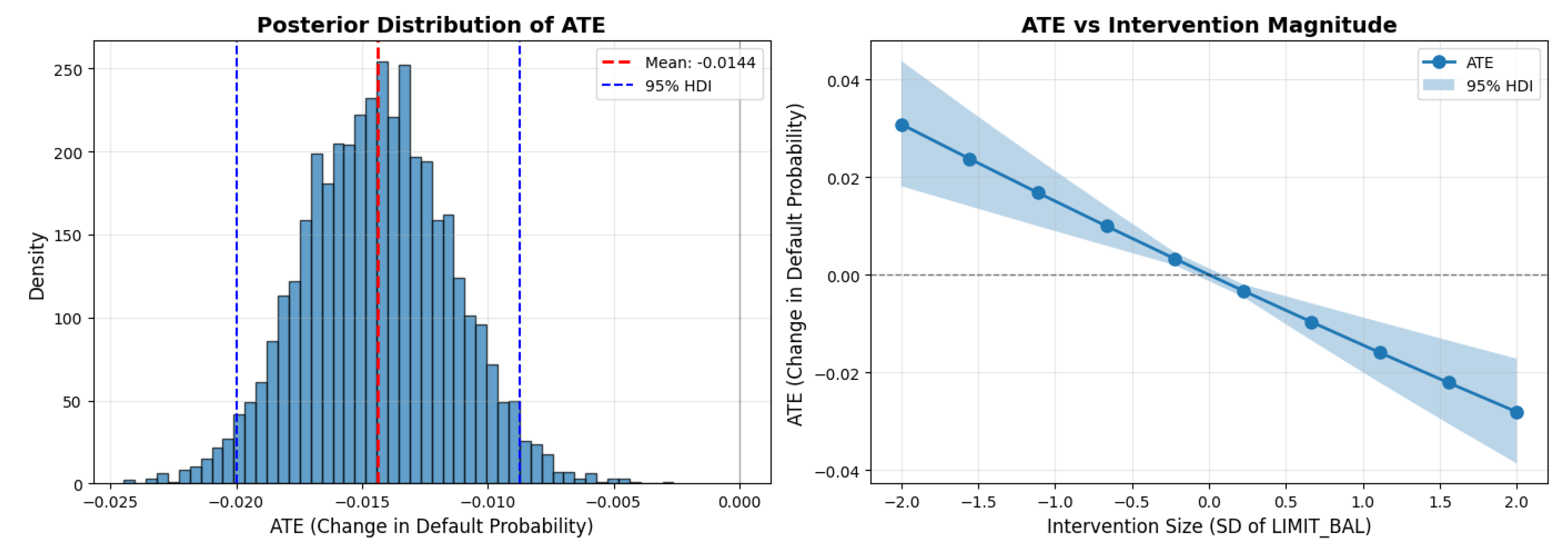
The ATE is -0.0144 (95% HDI: [-0.020, -0.010]), meaning a one standard deviation increase in credit limit (roughly NT$100,000) causes a 1.44 percentage point drop in default probability. This represents a 6.3% relative reduction in defaults, dropping the baseline rate from 22.1% to a counterfactual rate of 20.7% under intervention.
Figure 1.
Average Treatment Effect analysis. Left: Posterior distribution of the ATE (mean -0.0144; 95% HDI [-0.020, -0.010]), indicating a consistently negative and protective effect. Right: Dose–response curve illustrating that larger credit limit increases lead to proportionally greater reductions in default risk.
3.3. Conditional Average Treatment Effects

Table 2.
Conditional Average Treatment Effects by demographic subgroup.
| Subgroup | N | CATE Mean | 95% HDI |
|---|---|---|---|
| Age | 11,013 | -0.0150 | [-0.020, -0.010] |
| Age 31–50 | 16,718 | -0.0142 | [-0.019, -0.009] |
| Age >50 | 2,269 | -0.0148 | [-0.021, -0.009] |
| Graduate School | 10,585 | -0.0131 | [-0.018, -0.008] |
| University | 14,030 | -0.0144 | [-0.019, -0.009] |
| High School | 4,917 | -0.0143 | [-0.020, -0.009] |
| Male | 11,888 | -0.0141 | [-0.019, -0.009] |
| Female | 18,112 | -0.0145 | [-0.020, -0.009] |
Figure 2.
Conditional Average Treatment Effect analysis by demographic subgroups. Left: Forest plot of CATE estimates with 95% credible intervals, all overlapping and excluding zero. Right: Posterior distributions showing generally homogeneous treatment effects across age, education, and gender groups.

3.4. Model Validation
Figure 3.
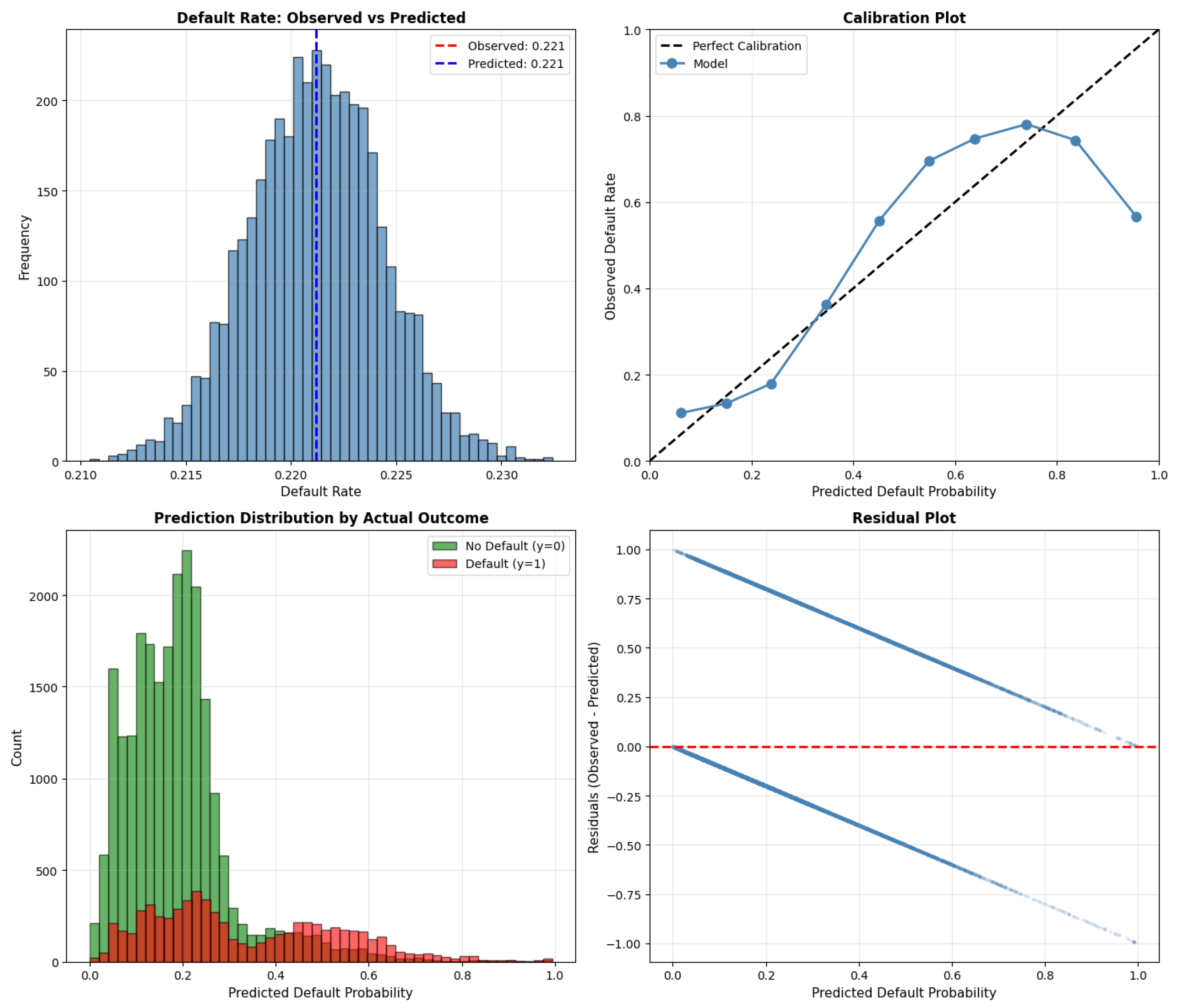
Posterior predictive checks for model validation. Predicted default rate matches the observed 22.1%. Calibration is strong with minor edge deviations. Predicted probabilities show good discrimination between defaulters and non-defaulters. Residuals exhibit a mild V-shape, suggesting remaining nonlinearities.
Figure 3.
Posterior predictive checks for model validation. Predicted default rate matches the observed 22.1%. Calibration is strong with minor edge deviations. Predicted probabilities show good discrimination between defaulters and non-defaulters. Residuals exhibit a mild V-shape, suggesting remaining nonlinearities.
3.5. Sensitivity Analysis
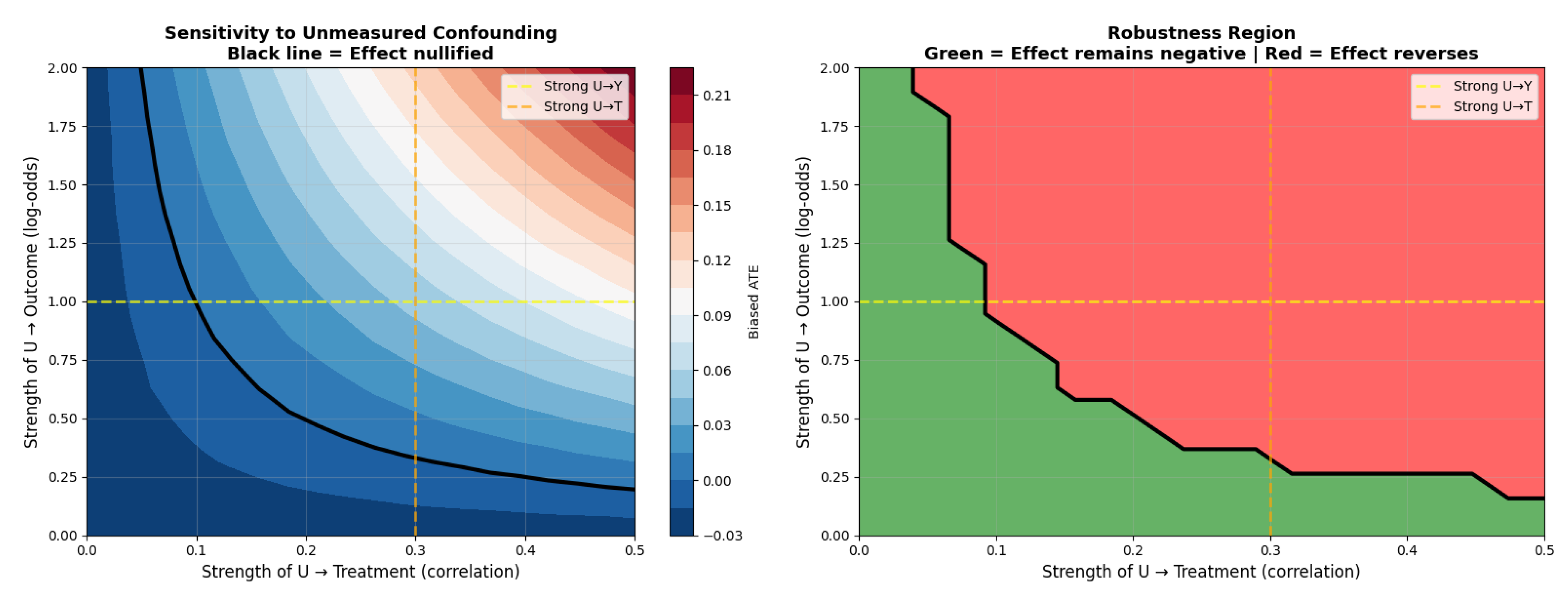
To completely nullify the observed ATE of percentage points, an unmeasured confounder would need to be strongly associated with both the treatment and the outcome. Specifically, it would require a correlation with credit limit assignment of at least and an effect on default probability of on the log-odds scale, which is substantially larger than the effects of any measured covariates. The corresponding E-value of approximately 1.15 further indicates that only a confounder of considerable strength could plausibly eliminate the observed causal effect.
Figure 4.
Sensitivity analysis for unmeasured confounding. Left: Bias-adjusted ATE across confounder strengths, with the nullification boundary marked in black; the dominant negative region indicates strong robustness. Right: Robustness (green) versus reversal (red) regions.
Figure 4.
Sensitivity analysis for unmeasured confounding. Left: Bias-adjusted ATE across confounder strengths, with the nullification boundary marked in black; the dominant negative region indicates strong robustness. Right: Robustness (green) versus reversal (red) regions.
4. Discussion
4.1. Principal Findings
This study provides clear causal evidence that increasing a customer’s credit limit reduces their probability of default. The results show that a one standard deviation increase in credit limit leads to a causal reduction of 1.44 percentage points in default probability (95% HDI: [-2.0%, -1.0%]). The posterior intervals exclude zero, all parameters achieved perfect convergence (), and the effect was consistent across demographic subgroups defined by age, education, and gender. Moreover, sensitivity analyses indicate that the findings are robust even to strong forms of unmeasured confounding. Collectively, these results challenge the conventional assumption that higher credit limits inherently increase default risk.
Once confounding factors that simultaneously influence credit limit assignment and default behaviour are properly accounted for, the evidence instead indicates that higher limits exert a protective effect against default.
4.2. Causal Mechanisms
The protective effect likely works through several pathways. First, financial flexibility. Higher available credit allows customers to weather temporary income shocks without defaulting. It provides a buffer during unexpected expenses or income disruptions. Second, lower credit utilization ratios (balance divided by limit) improve credit scores, making it easier to access additional credit or refinance. Third, reduced financial stress from adequate credit availability enables better payment planning and decision-making. Finally, psychological factors matter; customers with adequate limits experience less anxiety about credit availability, potentially improving overall financial behavior.
4.3. Comparison with Existing Literature
These findings complement but extend existing credit risk research. Unlike predictive studies [1,2] that optimize classification accuracy, we establish causal relationships suitable for policy evaluation. Predictive models identify who is likely to default but can’t tell you whether interventions would change outcomes.
5. Conclusions
In this paper, we investigated the causal effect of credit limit increases on default risk using Bayesian causal inference. By combining DAG-based identification, Bayesian logistic regression, and posterior predictive simulation on a data set of 30,000 credit card clients, we estimated that a one standard deviation increase in credit limit reduces default probability by 1.44 percentage points. The results provide clear evidence that after adjusting for key confounders, higher credit limits have a protective causal effect on default outcomes.
Compared with existing research, which has largely focused on predictive modeling rather than causal mechanisms, our findings extend the literature by isolating the effect of changes in the credit limit rather than simply identifying correlates of default. Earlier work has shown strong associations between credit behaviour and default risk, but few studies have applied formal causal frameworks to this policy question. Our results therefore contribute a more rigorous understanding of how credit limit policies influence customer outcomes.
Practically, these findings suggest that strategically increasing credit limits may reduce default rates by improving customers’ financial flexibility and lowering utilization ratios. This insight can assist lenders in designing data-informed credit strategies, refining risk management policies, and implementing targeted limit adjustments that balance customer support with regulatory and portfolio considerations.
Although the analysis provides strong evidence for a causal effect, several important aspects remain unexplored. The study focuses on data from a single financial institution during a specific historical period, which means that broader variation in economic environments or institutional practices was not examined. Moreover, while sensitivity analyses suggest robustness to unmeasured confounding, the possibility of omitted factors influencing both credit limit assignment and default behavior cannot be fully discounted.
Future research could extend this work by examining nonlinear or heterogeneous treatment effects, replicating the analysis across diverse lenders and economic contexts, and evaluating dynamic or longitudinal credit limit adjustments. Exploring mechanisms in more detail, such as behavioral responses or changes in utilization patterns, may also provide deeper insight into how credit limit policies shape default risk.
Author Contributions
Conceptualization, S.D.P.; methodology, S.D.P.; software, S.D.P.; validation, T.M.; formal analysis, S.D.P.; investigation, S.D.P.; resources, S.D.P.; data curation, S.D.P.; writing: original draft preparation, S.D.P.; writing: review and editing, T.M.; visualization, S.D.P.; supervision, T.M.; project administration, T.M. All authors have read and agreed to the published version of the manuscript.
Funding
This research received no external funding.
Institutional Review Board Statement
Not applicable. This study uses publicly available secondary data.
Informed Consent Statement
Not applicable.
Data Availability Statement
The data used in this study are publicly available. The credit default dataset can be accessed from Kaggle: https://www.kaggle.com/datasets/uciml/default-of-credit-card-clients-dataset. Analysis code is available at: https://github.com/pitsojaden/Bayesian-Causal-Analysis—Credit-Default.git.
Acknowledgments
The authors acknowledge the use of Claude (Anthropic) for assistance with literature review organization and LaTeX formatting. The authors have reviewed and edited all output and take full responsibility for the content of this publication.
Conflicts of Interest
The authors declare no conflicts of interest.
Abbreviations
The following abbreviations are used in this manuscript:
| ATE | Average Treatment Effect |
| CATE | Conditional Average Treatment Effect |
| DAG | Directed Acyclic Graph |
| ESS | Effective Sample Size |
| HDI | Highest Density Interval |
| MCMC | Markov Chain Monte Carlo |
| NUTS | No-U-Turn Sampler |
| SUTVA | Stable Unit Treatment Value Assumption |
References
- Kim, H.; Sohn, S.Y. Deep learning based on multi-task learning for credit default prediction. Expert Systems with Applications 2020, 149, Article 113306. [CrossRef]
- Wang, H.; Xu, Q.; Zhou, L. Large unbalanced credit scoring using lasso-logistic regression ensemble. PLoS ONE 2021, 16(2), Article e0246598. [CrossRef]
- Pearl, J. Causality: Models, Reasoning, and Inference, 2nd ed.; Cambridge University Press: Cambridge, UK, 2009.
- Hernán, M.A.; Robins, J.M. Causal Inference: What If; Chapman & Hall/CRC: Boca Raton, FL, USA, 2020.
- Fuster, A.; Goldsmith-Pinkham, P.; Ramadorai, T.; Walther, A. Predictably unequal? The effects of machine learning on credit markets. Journal of Finance 2021, 77(1), 5–47. [CrossRef]
- Dobbie, W.; Goldsmith-Pinkham, P.; Mahoney, N.; Song, J. Bad credit, no problem? Credit and labor market consequences of bad credit reports. Journal of Finance 2020, 75(5), 2377–2419. [CrossRef]
- Imbens, G.W.; Rubin, D.B. Causal Inference for Statistics, Social, and Biomedical Sciences: An Introduction; Cambridge University Press: Cambridge, UK, 2015.
- Hoffman, M.D.; Gelman, A. The No-U-Turn sampler: Adaptively setting path lengths in Hamiltonian Monte Carlo. Journal of Machine Learning Research 2014, 15, 1593–1623.
- Gelman, A.; Carlin, J.B.; Stern, H.S.; Dunson, D.B.; Vehtari, A.; Rubin, D.B. Bayesian Data Analysis, 3rd ed.; CRC Press: Boca Raton, FL, USA, 2013.
- VanderWeele, T.J.; Ding, P. Sensitivity analysis in observational research: Introducing the E-value. Annals of Internal Medicine 2017, 167(4), 268–274. [CrossRef]
- Lessmann, S.; Baesens, B.; Seow, H.V.; Thomas, L.C. Benchmarking state-of-the-art classification algorithms for credit scoring. European Journal of Operational Research 2015, 247(1), 124–136. [CrossRef]
- Kvamme, H.; Sellereite, N.; Aas, K.; Sjursen, S. Predicting mortgage default using convolutional neural networks. Expert Systems with Applications 2018, 102, 207–217. [CrossRef]
Table 1.
Posterior summary statistics for key model parameters.
| Parameter | Mean | SD | HDI 3% | HDI 97% | ESS | |
|---|---|---|---|---|---|---|
| Intercept () | -1.468 | 0.016 | -1.499 | -1.439 | 6356 | 1.0 |
| Treatment () | -0.099 | 0.020 | -0.137 | -0.061 | 6510 | 1.0 |
Disclaimer/Publisher’s Note: The statements, opinions and data contained in all publications are solely those of the individual author(s) and contributor(s) and not of MDPI and/or the editor(s). MDPI and/or the editor(s) disclaim responsibility for any injury to people or property resulting from any ideas, methods, instructions or products referred to in the content. |
© 2025 by the authors. Licensee MDPI, Basel, Switzerland. This article is an open access article distributed under the terms and conditions of the Creative Commons Attribution (CC BY) license (http://creativecommons.org/licenses/by/4.0/).
Copyright: This open access article is published under a Creative Commons CC BY 4.0 license, which permit the free download, distribution, and reuse, provided that the author and preprint are cited in any reuse.


