
Submitted:
23 November 2025
Posted:
24 November 2025
You are already at the latest version
Abstract
Gas flaring in oil and gas facilities prevents pressure buildup and ensures safety, but large-scale flaring emits significant greenhouse gases and contributes to climate change. Detecting and monitoring gas flaring are crucial for mitigating its impact. Satellite imagery offers key advantages for these tasks, including open data availability, global coverage, and broad spectral capture. However, despite the availability of flame and smoke datasets, as well as hyperspectral data for methane emissions, there is a lack of open hyperspectral satellite datasets and deep learning approaches for gas flaring detection. To address this gap, we introduce FlareSat, a specialized dataset for gas flaring segmentation using Landsat 8 imagery. It includes 7,337 labeled image patches (256 X 256 pixels) covering 5,508 facilities across 94 countries, including onshore and offshore sites, making it a valuable resource for future research. Additionally, to ensure robustness, the dataset includes patches featuring sources similar to gas flaring, namely wildfires, active volcanoes, and urban areas with high solar reflectance. To evaluate the dataset, we used a baseline semantic segmentation model along with variations, exploring attention layers and transfer learning. Results showed that specialized machine learning techniques enhance the ability to distinguish between gas flares and other high-temperature sources.
Keywords:
gas flare
; remote sensing
; satellite image
; deep learning
1. Introduction
Gas flaring is a widespread practice in the oil industry, resulting from technical and economic barriers to utilizing or storing associated gas [1,2]. This process is a major source of greenhouse gas emissions [3]. Incomplete combustion exacerbates the problem by releasing methane [4], and the practice poses significant environmental, economic, and public health challenges [5]. Accurate detection of flaring activity is, therefore, crucial for emissions monitoring. However, effective detection is hindered by challenges such as the remote location of facilities, inconsistent reporting, and a lack of reliable open data [6].
To address these challenges, remote sensing has become a key resource. Satellites equipped with a range of spectral and infrared sensors provide imagery capable of capturing the heat signatures of gas flaring activity [7] and offer significant advantages, including global coverage and persistent monitoring capabilities [8]. These sensors demonstrate their potential, particularly for short-wave infrared (SWIR) bands, where gas flaring is distinctly visible [9].
To achieve more precise identification, semantic segmentation of satellite imagery has been developed for pixel-level localization [10,11]. However, accurate fine-grained segmentation is hindered by challenges such as the small size of flares and atmospheric effects, including light scattering. These phenomena increase radiance around heat sources, reduce contrast, and consequently cause significant false detections in traditional algorithms that rely on contrast, thresholding, and spectral characteristics [7].
Deep learning methods for methane plume segmentation using hyperspectral data show promise [12], but they rely on datasets that are often limited in size and scene variety, or are based on simulated data, which may lack realistic variability [12]. Although methane plumes can indicate inefficient flaring (i.e., incomplete combustion), not all flares emit methane. Flaring typically produces visible light, heat, and noise, and—when combustion is efficient—mainly CO2 and water vapor. Combustion efficiency depends on proper mixing between the fuel gas and air (or steam) and on the absence of liquids in the flare system; low-pressure flares perform poorly when hydrocarbons enter as liquids [6]. Even when methane emissions are minimal, flares can still generate other pollutants, such as carbon monoxide and black carbon, especially when mixing is inadequate or liquids are present [6].
To address data limitations, we introduce FlareSat, an open dataset for gas flaring segmentation from Landsat 8 imagery. The dataset contains 7,337 image patches ( pixels), capturing flaring activity at 5,508 onshore and offshore facilities across 94 countries.
For robust evaluation, the data are partitioned into geographic folds to assess model generalization and reduce spatial autocorrelation [13]. To introduce realistic segmentation challenges, patches containing wildfires and urban areas with high solar reflectance—common sources of false positives—were also included [7,14].
We benchmarked U-Net [15] and its variants, including attention mechanisms and transfer learning from Sentinel-2 for land cover segmentation. While modern architectures, such as transformers, perform well in remote sensing, U-Net provides an efficient baseline for the continent-spanning FlareSat dataset. Our experiments demonstrate that deep learning improves gas flaring segmentation and provides a foundation for the future evaluation of more complex models.
Overall, this work makes the following contributions:
- we introduce and publicly release FlareSat, which, as far as we are concerned, is the first open-access dataset for gas flaring segmentation from multispectral satellite imagery The dataset includes challenging false positive samples, namely wildfires and urban highly reflective areas;
- we propose a spatial cross-validation framework to assess a model’s generalization across continents and to mitigate spatial bias;
- we provide benchmark results demonstrating that deep learning models improve flaring segmentation accuracy and reduce false positives.
2. Related Work
Most datasets for gas flare activity segmentation rely on RGB terrestrial cameras, mainly for monitoring flame composition and smoke [16]. Even though remote sensing offers broader temporal coverage, a global scale, and richer spectral bands [7], the available datasets remain limited.
Hyperspectral techniques have been applied to gas flare detection using sensors such as VIIRS, Landsat 8, and Sentinel-2/-3 [7]. VIIRS Nightfire [17] is widely used, but its coarse spatial resolution (750 m/pixel) and sensitivity to atmospheric interference limit its effectiveness for segmentation.
Methods such as the Normalized Hotspot Index (NHI) [18] and the Thermal Anomaly Index (TAI) [11] were used for gas flare detection in Sentinel-2 and Landsat 8 images. NHI, based on band subtraction and persistence, struggles with low-temperature sources and misclassifications [18], while TAI uses contrast-based thresholding but depends on urban masks to limit false positives, thereby reducing global applicability.
The Reed-Xiaoli Detector (RXD) was applied to isolate gas flare anomalies in Operational Land Imager (OLI) sensor images [10]. Despite being visually validated, its reliance on limited scenes and computational complexity limits large-scale application, requiring significant processing power, particularly with large datasets.
Methane emissions from gas flaring are closely linked to flare combustion efficiency. Ideally, flaring oxidizes methane into carbon dioxide and water, reducing emissions compared to direct venting [6]. However, even under optimal conditions, flares release greenhouse gasses such as carbon monoxide, and inefficient combustion or equipment leaks—caused by extinguished pilots, high crosswinds, or malfunctions—can emit significant amounts of unburned methane [4].
These emissions appear as methane plumes in the atmosphere, which can be mapped using deep learning segmentation that leverages the spectral sensitivity of satellites such as Sentinel-2, AVIRIS-NG, GHGSat-C1, and PRISMA. The plumes often coincide with flare sites, reflecting incomplete combustion and fugitive leaks, highlighting the value of satellite observations for accurate methane emission datasets [4,12].
AVIRIS-NG [19] used methane enhancement maps and RGB channels instead of full hyperspectral data, limiting spectral detail, and achieved only 45% F1 when classifying plumes as weak, medium, or strong[12].
GHGSat’s U-Plume model [20], trained on simulated plumes in random scenes, showed few false positives—mainly in complex topography—but its reliance on synthetic data limits diversity and realism compared to real-world conditions [12].
PRISMethaNet [21] demonstrated potential for methane segmentation on PRISMA data but was limited by a small dataset (41 patches, expanded to 1,585 through augmentation). Similarly, a Sentinel-2 approach [22] generated one million synthetic plumes, achieving high performance but constrained by the reduced diversity, characteristics, and real-world conditions of the synthetic samples [12].
In summary, traditional threshold-based techniques for flare segmentation often produce false positives [7]. Deep learning methods for flare and methane segmentation face similar challenges due to the lack of large-scale, diverse, and open benchmark datasets. Progress is further limited by scarce real annotations, restricted geographic coverage, and, for methane segmentation, a heavy reliance on synthetic data that provides limited representation of real-world variability [12].
3. Dataset
This section presents the dataset developed for gas flaring segmentation, detailing its collection, preprocessing, and annotation procedures.
3.1. Preprocessing
The study by the Suomi National Polar-Orbiting Partnership (Suomi NPP) was utilized to retrieve the geographic locations of flares detected using the VIIRS Nightfire (VNF) [23]. We focused on data from 2019, a year with a significant increase in pollution from gas flaring [24,25] with 8,098 unique flare locations mapped in the study [17] – each location defined by a latitude–longitude point.
Landsat 8 satellite scenes from 2019 were used to match the flare locations. Specifically, scenes from March, August, September, and December with less than 10% cloud coverage were selected to identify each gas flare point reported by the VIIRS Nightfire study. The Landsat 8 images were used for their high spatial resolution, which improves flare visibility [9]. The satellite provides 11 spectral bands at a 30-meter resolution and one band (B8) at a 15-meter resolution. B8 was excluded from the dataset due to its lower spectral relevance for gas flare segmentation and the potential for artifacts or noise resulting from resampling the higher-resolution 15-meter band to match the 30-meter bands [7]. A total of 3,809 Landsat 8 scenes were obtained, each covering approximately 250 km2. To reduce image size for training, the scenes were divided into patches of 256 × 256 pixels.
Active-fire [14], a method based on the U-Net with a voting scheme for segmentation, was applied to the patches to annotate pixels associated with gas flaring (see Figure 1). Patches with at least three fire-classified pixels were selected, a threshold determined by the observed size of the model’s output.
3.2. Labeling
Flare areas were labeled by square regions of 7 × 7 to 37 × 37 pixels (ranging approximately from 210 m2 to 1.1 km2), around their locations. These sizes are based on the VIIRS gas flaring study [23]. To ensure accuracy, images containing fire pixels outside predefined flare locations were discarded. Figure 2 illustrates a sample patch with two flare locations: one active and one inactive. A patch is included in the dataset if at least one of the flares has active combustion, as indicated by Active-fire.
3.3. Wildfires and Urban Surfaces
To introduce variability to the flare dataset, manually annotated Landsat 8 wildfire and controlled burn patches from [14] were included (see Figure 3), provided that they did not overlap with existing gas flaring patches. Since the dataset focuses on gas flaring, these patches were masked as background (set to zero).
Highly reflective urban surfaces, such as industrial rooftops, can be misclassified as fire events due to intense sunlight reflections [14]. To mitigate this issue, additional patches containing urban areas have been added to the dataset. These patches were selected by ranking the 450 most populated cities worldwide, obtaining their geographic coordinates [26], and matching them with the corresponding Landsat scenes. To avoid overlap with known flare locations, cities located within a 10 km radius of any flare coordinates were excluded. Furthermore, patches were filtered to ensure that cloud coverage was below 10%. The masks for these regions were also set to zero.
3.4. Spatial Split of the Dataset
The same locations with gas combustion, captured in images taken on different days, can introduce data redundancy. The dataset includes 5,508 locations: 3,252 appear once, and 2,256 appear more frequently (1.88 occurrences on average). To prevent evaluation bias and reduce spatial dependence related to surface and land characteristics, we propose a spatial cross-validation strategy [13] to ensure a comprehensive and geographically diverse evaluation.
The dataset was partitioned into four folds based on major continental regions: (1) Asia, (2) Africa, (3) North America & Oceania, and (4) Europe & South America. In each fold iteration, one region (e.g., Fold 4) is held out exclusively for testing, while the remaining three folds (e.g., Folds 1, 2, and 3) are used for model training and validation. Specifically, the images from these three folds are randomly split internally – 10% for validation and the remaining 90% for training. A trained model is evaluated on the entire held-out continent fold. The process is repeated four times, allowing each geographic region to serve once as the evaluation set.
For the urban patches, the dataset was divided into four groups of cities. Since most highly populated cities are located in Asia, a purely continent-based fold split would have led to an imbalanced distribution. To address this, the folds are defined based on city groups rather than continents. This approach ensures that cities used for training are excluded from the testing phase. Wildfire samples are randomly distributed among the 4 folds.
3.5. Statistics of the Dataset
Table 1 summarizes the number of patches and pixels per fold. Flare samples dominate the dataset, ranging from 1,261 to 2,990 patches per fold, whereas wildfire and urban samples remain relatively stable at around 65–67 patches per fold. When looking at pixel counts, Fold 1 (Asia) contributes the largest number of flare-related pixels, clearly dominating the distribution. In Fold 2 (Africa), however, wildfire pixels become the most prominent component, with a much higher count than in the other folds. Fold 4 (Europe & South America) shows a more balanced distribution between flare and wildfire pixels, while Fold 3 (North America & Oceania) follows a pattern similar to Fold 2, with wildfire pixels exceeding flare pixels. Urban highly reflective surface pixels remain fairly consistent across folds, with only an increase in Fold 2, where they deviate from the overall trend.
Figure 4 presents the distribution of blob sizes across the different folds. Wildfires exhibit larger average blob sizes. Gas flares show a more uniform blob size distribution, as combustion-related regions tend to follow a consistent pattern. Urban areas, on the other hand, have smaller average blob sizes.
In addition to the quantitative pixel statistics previously presented, we examined the geographical distribution of the dataset, which is highly diverse. Fold 1 (Asia) contains 2,015 unique locations across 28 countries; Fold 2 (Africa) includes 815 locations in 17 countries; Fold 3 (North America & Oceania) comprises 3,235 locations among 12 countries; and Fold 4 (South America & Europe) holds 1,951 locations across 23 countries. These numbers differ from the total number of flare patches (7,337), as multiple nearby locations can be captured within the same patch.
4. Experiments
Models were tested with different input configurations of Landsat 8: all bands, selected three-band sets (B2, B6, B7; B5, B6, B7), and a four-band set (B4, B5, B6, B7). The variations of the selected bands are based on prior work to detect high-energy gas combustion emissions [7]. Although more complex architectures exist, U-Net and its variants remain state-of-the-art for segmentation and provide an initial baseline. We therefore focus on four U-Net variants to benchmark our multi-continent dataset across folds, architectures, and spectral bands. More advanced models can be explored in future work.
The U-Net [15] baseline used an input size of 256×256 ( according to the number of selected bands) and encoder dimensions of 32, 64, 128, 256, and 512. The Attention U-Net [27] was included to assess the preservation of fine details often lost through pooling [28]. Transfer learning was tested with the Land Cover U-Net, leveraging Sentinel-2 pretraining on 11 land cover classes [29]. Sentinel-2 bands (bands B2-B8, B11, and B12) were mapped to Landsat-8 (B2-B7), while unmatched bands were initialized using He’s kernel [30]. Output layers were adapted for binary classification. Finally, the Att-Land Cover U-Net combined the same transfer learning on land cover classes with attention mechanisms.
All architectures had 7–11 million parameters and were trained for 100 epochs with a batch size of 16. The learning rate was 0.001 for most models and 0.0005 for Attention U-Net. To address class imbalance due to the small proportion of flaring pixels, we used Focal Loss [31], which emphasizes difficult-to-classify examples. Parameter updates were performed with the Adam optimizer [32]. Experiments were run on an NVIDIA RTX 4070 GPU (8 GB), an Intel Core i7-13700HX (30M Cache, up to 5.00 GHz), and 32 GB of RAM.
4.1. Evaluation of Semantic Segmentation Models
Table 2 presents the highest F1 scores achieved by each network for the different band combinations. The evaluation considered all patches, including flare, wildfire, and urban reflectances. Across all tested architecture configurations and spectral band combinations, performance was comparable for the evaluated metrics. The base U-Net has already achieved good results, demonstrating its capacity to learn relevant patterns. Incorporating attention (Att-U-Net) slightly improved F1 for B2, B6, B7 in Folds 2 and 3. In contrast, for Fold 1, the baseline U-Net performed slightly better, and in Fold 4, it outperformed the attention-enhanced model.
The Land Cover U-Net (LC U-Net) model achieved a lower mean F1 score compared to both the standard U-Net and its variant with the attention mechanism. The best performance was obtained with the B4, B5, B6, and B7 band combination, which corresponds to the configuration in which all Sentinel-2 bands were used in the transfer learning process. This indicates that pre-trained weights alone did not improve learning on this dataset. Although Sentinel-2 bands were mapped to their corresponding Landsat 8 bands, differences in the capture intervals of the sensors and spatial resolutions may have impacted the results.
The addition of the attention mechanism to the transfer learning approach (Att-LC U-Net) achieved the best mean F1 score with the all bands configuration (B1-B10). However, the scores remained lower than the base U-Net’s top performance. Therefore, not even the attention mechanisms combined with transfer learning were able to outperform the simpler baseline.
When comparing the performance across the best band combinations, some regional differences can be observed. The best model overall, U-Net with B2, B6, and B7, achieved the highest F1 scores for Fold (1) – Asia and Fold (4) - South America & Europe. In Fold (1), the performance gain over the other architectures is slight; however, when compared to the transfer learning approaches, the improvement is more substantial. For Fold (4), the baseline U-Net achieved better results than the other models, which showed similar performance to each other.
For Fold (2) - Africa and Fold (3) - North America & Oceania, the Att-U-Net with the B2, B6, and B7 combination bands slightly outperformed both the baseline U-Net. However, the Land Cover U-Net showed a drop in Fold (3) compared to the other approaches. For the band combinations in the transfer learning approaches, neither the B4, B5, B6, and B7 combination used in the Land Cover U-Net nor the full B1–B10 combination used in the Att-Land Cover U-Net improved the results across the four folds, as both the U-Net and Att-U-Net outperformed them.
To assess whether differences in F1 scores across models were statistically significant, we performed paired t-tests for all pairwise comparisons across folds and applied a Bonferroni correction () to account for multiple testing. After correction, no significant differences were observed in F1 scores across folds.
Figure 5 shows the predictions of the best-performing models for each architecture using their optimal band combination. The yellow square highlights the gas flare region, which is magnified in the segmentation outputs.
4.2. Evaluation of False Positives Scenarios
Given similar overall model performance, we evaluated false positives for wildfires and urban areas using the best-performing band combination for each architecture. Because these cases have zero masks, metrics such as accuracy and sensitivity are uninformative due to the small number of false positives relative to true negatives. Consequently, we focused on visual inspection and a quantitative analysis of false positives.
Table 3 presents the results of this analysis, highlighting the models with the lowest false positive rates per fold for both wildfire and urban categories. The False Positive Rate (FPR) was computed by dividing the number of false positive pixels predicted by the model for each category (Wildfire and Urban) within each continent-based evaluation fold by the total number of negative (non-flare) pixels in that category:
For U-Net, we observed good results in reducing wildfire-related false positives across all folds, with only minor deviations in Folds 2 and 4. Att-U-Net showed results similar to the transfer learning approach, Land Cover U-Net (LC U-Net), in Fold 1 but underperformed in Fold 4 compared to other architectures. Focusing only on transfer learning approaches, both models achieved their best performance in Fold 4 compared to models trained without transfer learning. The LC U-Net performed comparably to non-transfer models in Folds 2 and 3, whereas the Att-LC U-Net showed lower performance in Fold 1. Figure 6 illustrates a wildfire patch from Fold 3, with the yellow square highlighting the wildfire region and the zoomed-in views showing the segmented pixels.
For urban areas, U-Net outperformed other architectures only in Fold 4, while it underperformed in Fold 2. Att-U-Net generally lagged behind; however, in Fold 1, it achieved results comparable to U-Net. LC U-Net performed best in Folds 1 and 2, showed a slight difference from the baseline U-Net in Fold 3, and was nearly equal to Att-U-Net in Fold 4. Att-LC U-Net exhibited the weakest performance in Folds 1 and 4, but it outperformed non-transfer learning models in Fold 2 and all other architectures in Fold 3. Figure 7 provides a visual comparison of the outputs.
Although urban highly reflective surfaces exhibit distinct temperature and spectral emission when compared to gas flares, spectral values in the B6 and B7 bands can be similar due to the limited dynamic range of the Landsat OLI sensors, which often leads to pixel saturation in regions with intense thermal emissions [9].
5. Conclusions
The limited availability of diverse annotated datasets has constrained deep learning approaches for gas flaring detection. To address this, we developed FlareSat, a labeled Landsat 8 dataset with continent-based cross-validation. Our results showed that the models generally reduced false positives in wildfire areas, with the baseline U-Net performing well and the transfer learning variants outperforming it in one fold. Urban regions remain challenging due to Landsat’s limited dynamic range.
By leveraging publicly available satellite imagery, FlareSat provides a valuable resource for global gas flaring monitoring, and the trained models establish a framework for the automated detection and monitoring of flaring activity. Future work could address the limitations observed with transfer learning by exploring domain adaptation techniques [33] and pretraining on datasets more closely aligned with Landsat 8, as well as investigating alternative network architectures to further improve segmentation performance.
Author Contributions
Osmary Camila Bortoncello Glober designed and conducted the experiments, performed data analysis, and drafted the manuscript. Ricardo Dutra da Silva contributed to the study’s conception and refinement, supervised the analysis, interpreted the results, and reviewed and edited the manuscript. All authors have read and approved the final version of the manuscript.
Data Availability Statement
The datasets and software generated or analyzed during the current study are available at http://github.com/marycamila184/flaresat.
Conflicts of Interest
The authors declare that they have no competing financial or non-financial interests.
References
- Elvidge, C.D.; Bazilian, M.D.; Zhizhin, M.; Ghosh, T.; Baugh, K.; Hsu, F.C. The potential role of natural gas flaring in meeting greenhouse gas mitigation targets. Energy strategy reviews 2018, 20, 156–162. [Google Scholar] [CrossRef]
- Ialongo, I.; Stepanova, N.; Hakkarainen, J.; Virta, H.; Gritsenko, D. Satellite-based estimates of nitrogen oxide and methane emissions from gas flaring and oil production activities in Sakha Republic, Russia. Atmospheric Environment: X 2021, 100114. [Google Scholar] [CrossRef]
- Ismail, O.S.; Umukoro, G.E. Global impact of gas flaring. Energy and Power Engineering 2012, 4, 290–302. [Google Scholar] [CrossRef]
- Plant, G.; Kort, E.A.; Brandt, A.R.; Chen, Y.; Fordice, G.; Gorchov Negron, A.M.; Schwietzke, S.; Smith, M.; Zavala-Araiza, D. Inefficient and unlit natural gas flares both emit large quantities of methane. Science 2022, 377, 1566–1571. [Google Scholar] [CrossRef]
- Mirrezaei, M.A.; Orkomi, A.A. Gas flares contribution in total health risk assessment of BTEX in Asalouyeh, Iran. Process Safety and Environmental Protection 2020, 137, 223–237. [Google Scholar] [CrossRef]
- Emam, E.A. Gas Flaring in Industry: An Overview. Petroleum & Coal 2015, 57, 532–555. [Google Scholar]
- Faruolo, M.; Caseiro, A.; Lacava, T.; Kaiser, J.W. Gas Flaring: A Review Focused On Its Analysis From Space. IEEE Geoscience and Remote Sensing Magazine 2020, 9, 258–281. [Google Scholar] [CrossRef]
- Elvidge, C.D.; Ziskin, D.; Baugh, K.E.; Tuttle, B.T.; Ghosh, T.; Pack, D.W.; Erwin, E.H.; Zhizhin, M. A fifteen year record of global natural gas flaring derived from satellite data. Energies 2009, 2, 595–622. [Google Scholar] [CrossRef]
- Soszynska, A. Parametrisation of Gas Flares Using FireBIRD Infrared Satellite Imagery. Ph.D. Thesis, Humboldt-Universität zu Berlin, 2021. [Google Scholar]
- Asadi-Fard, E.; Falahatkar, S.; Tanha Ziyarati, M.; Zhang, X.; Faruolo, M. Assessment of RXD algorithm capability for gas flaring detection through OLI-SWIR channels. Sustainability 2023, 15, 5333. [Google Scholar] [CrossRef]
- Wu, W.; Liu, Y.; Rogers, B.M.; Xu, W.; Dong, Y.; Lu, W. Monitoring gas flaring in Texas using time-series Sentinel-2 MSI and Landsat-8 OLI images. International Journal of Applied Earth Observation and Geoinformation 2022, 114, 103075. [Google Scholar] [CrossRef]
- Tiemann, E.; Zhou, S.; Kläser, A.; Heidler, K.; Schneider, R.; Zhu, X.X. Machine learning for methane detection and quantification from space-a survey. arXiv 2024, arXiv:2408.15122. [Google Scholar] [CrossRef]
- Rolf, E. Evaluation challenges for geospatial ML. arXiv 2023, arXiv:2303.18087. [Google Scholar] [CrossRef]
- de Almeida Pereira, G.H.; Fusioka, A.M.; Nassu, B.T.; Minetto, R. Active fire detection in Landsat-8 imagery: A large-scale dataset and a deep-learning study. ISPRS Journal of Photogrammetry and Remote Sensing 2021, 178, 171–186. [Google Scholar] [CrossRef]
- Ronneberger, O.; Fischer, P.; Brox, T. U-net: Convolutional networks for biomedical image segmentation. In Proceedings of the Medical image computing and computer-assisted intervention–MICCAI 2015: 18th international conference, Munich, Germany, October 5-9, 2015, proceedings, part III 18. Springer, 2015, pp. 234–241. 234–241. [CrossRef]
- Al Radi, M.; Li, P.; Boumaraf, S.; Dias, J.; Werghi, N.; Karki, H.; Javed, S. AI-Enhanced Gas Flares Remote Sensing and Visual Inspection: Trends and Challenges. IEEE Access 2024. [Google Scholar] [CrossRef]
- Elvidge, C.D.; Zhizhin, M.; Hsu, F.C.; Baugh, K.E. VIIRS Nightfire: Satellite pyrometry at night. Remote Sensing 2013, 5, 4423–4449. [Google Scholar] [CrossRef]
- Faruolo, M.; Falconieri, A.; Genzano, N.; Lacava, T.; Marchese, F.; Pergola, N. A daytime multisensor satellite system for global gas flaring monitoring. IEEE Transactions on Geoscience and Remote Sensing 2022, 60, 1–17. [Google Scholar] [CrossRef]
- Ruzzicka, V.; Mateo-Garcia, G.; Gomez-Chova, L.; Vaughan, A.; Guanter, L.; Markham, A. Semantic segmentation of methane plumes with hyperspectral machine learning models. Scientific Reports 2023, 13, 19999. [Google Scholar] [CrossRef]
- Bruno, J.H.; Jervis, D.; Varon, D.J.; Jacob, D.J. U-Plume: automated algorithm for plume detection and source quantification by satellite point-source imagers. Atmospheric Measurement Techniques 2024, 17, 2625–2636. [Google Scholar] [CrossRef]
- Marjani, M.; Mohammadimanesh, F.; Varon, D.J.; Radman, A.; Mahdianpari, M. PRISMethaNet: A novel deep learning model for landfill methane detection using PRISMA satellite data. ISPRS Journal of Photogrammetry and Remote Sensing 2024, 218, 802–818. [Google Scholar] [CrossRef]
- Rouet-Leduc, B.; Hulbert, C. Automatic detection of methane emissions in multispectral satellite imagery using a vision transformer. Nature Communications 2024, 15, 3801. [Google Scholar] [CrossRef]
- Elvidge, C.D.; Zhizhin, M.; Baugh, K.; Hsu, F.C.; Ghosh, T. Methods for global survey of natural gas flaring from visible infrared imaging radiometer suite data. Energies 2015, 9, 14. [Google Scholar] [CrossRef]
- World Bank. Global Gas Flaring Data. https://www.worldbank.org/en/programs/gasflaringreduction/global-flaring-data, 2023. Accessed: 2024-10-20.
- Institute, A.P. Reports: U.S. Among World Leaders in Reducing Flaring, 2022. accessed in 2024-03-02.
- SimpleMaps. World Cities Database, 2024. Accessed: 2025-02-02.
- Oktay, O.; Schlemper, J.; Folgoc, L.L.; Lee, M.; Heinrich, M.; Misawa, K.; Mori, K.; McDonagh, S.; Hammerla, N.Y.; Kainz, B.; et al. Attention u-net: Learning where to look for the pancreas. arXiv 2018, arXiv:1804.03999. [Google Scholar] [CrossRef]
- Bagwari, N.; Kumar, S.; Verma, V.S. A comprehensive review on segmentation techniques for satellite images. Archives of Computational Methods in Engineering 2023, 30, 4325–4358. [Google Scholar] [CrossRef]
- Mäyrä, J. Land cover classification from multispectral data using convolutional autoencoder networks. Master’s thesis, University of Jyväskylä, 2018.
- Datta, L. A survey on activation functions and their relation with Xavier and He normal initialization. arXiv 2020, arXiv:2004.06632. [Google Scholar] [CrossRef]
- Ross, T.Y.; Dollár, G. Focal loss for dense object detection. In Proceedings of the proceedings of the IEEE conference on computer vision and pattern recognition, 2017, pp. 2980–2988. [CrossRef]
- Kingma, D.P. Adam: A method for stochastic optimization. arXiv 2014, arXiv:1412.6980. [Google Scholar] [CrossRef]
- Liu, Y.; Zhang, W.; Wang, J. Source-free domain adaptation for semantic segmentation. In Proceedings of the Proceedings of the IEEE/CVF conference on computer vision and pattern recognition, 2021, pp. 1215–1224. [CrossRef]
Figure 1.
Segmentation of fire in patches to annotate the dataset. (a) RGB patch; (b) B7 band patch; (c) Active-fire model output, with fire-classified pixels in red.
Figure 1.
Segmentation of fire in patches to annotate the dataset. (a) RGB patch; (b) B7 band patch; (c) Active-fire model output, with fire-classified pixels in red.
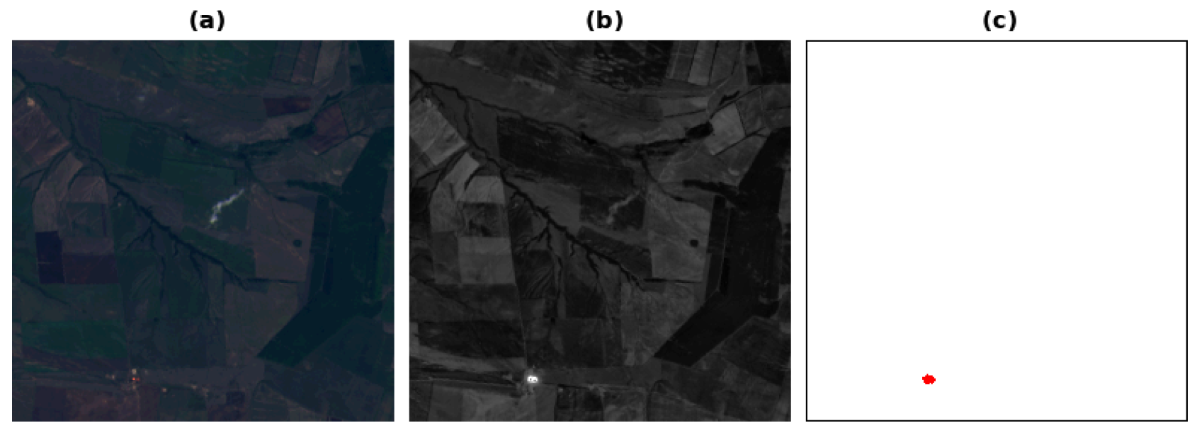
Figure 2.
Labeled patch. (a) RGB patch; (b) B7 band patch; (c) Active-fire model output, with fire-classified pixels in red and blue squares indicating the flare locations.
Figure 2.
Labeled patch. (a) RGB patch; (b) B7 band patch; (c) Active-fire model output, with fire-classified pixels in red and blue squares indicating the flare locations.
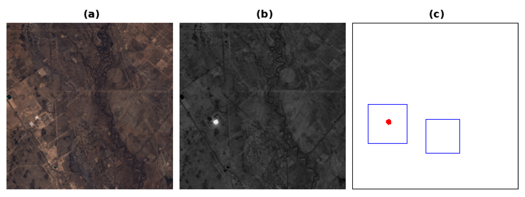
Figure 3.
Wildfire patch. (a) RGB patch; (b) B7 band patch; (c) Active-fire model output, with fire-classified pixels highlighted in red.
Figure 3.
Wildfire patch. (a) RGB patch; (b) B7 band patch; (c) Active-fire model output, with fire-classified pixels highlighted in red.
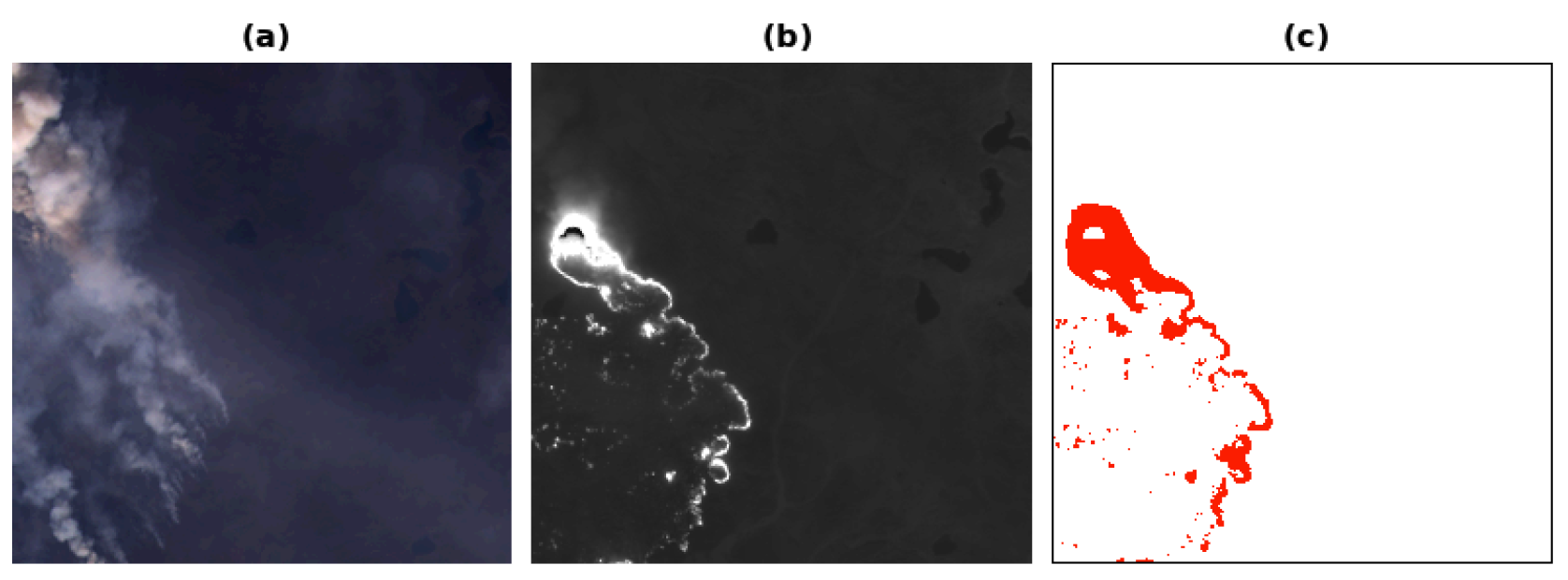
Figure 4.
Distribution of blob sizes in each fold, with red triangles indicating mean values.
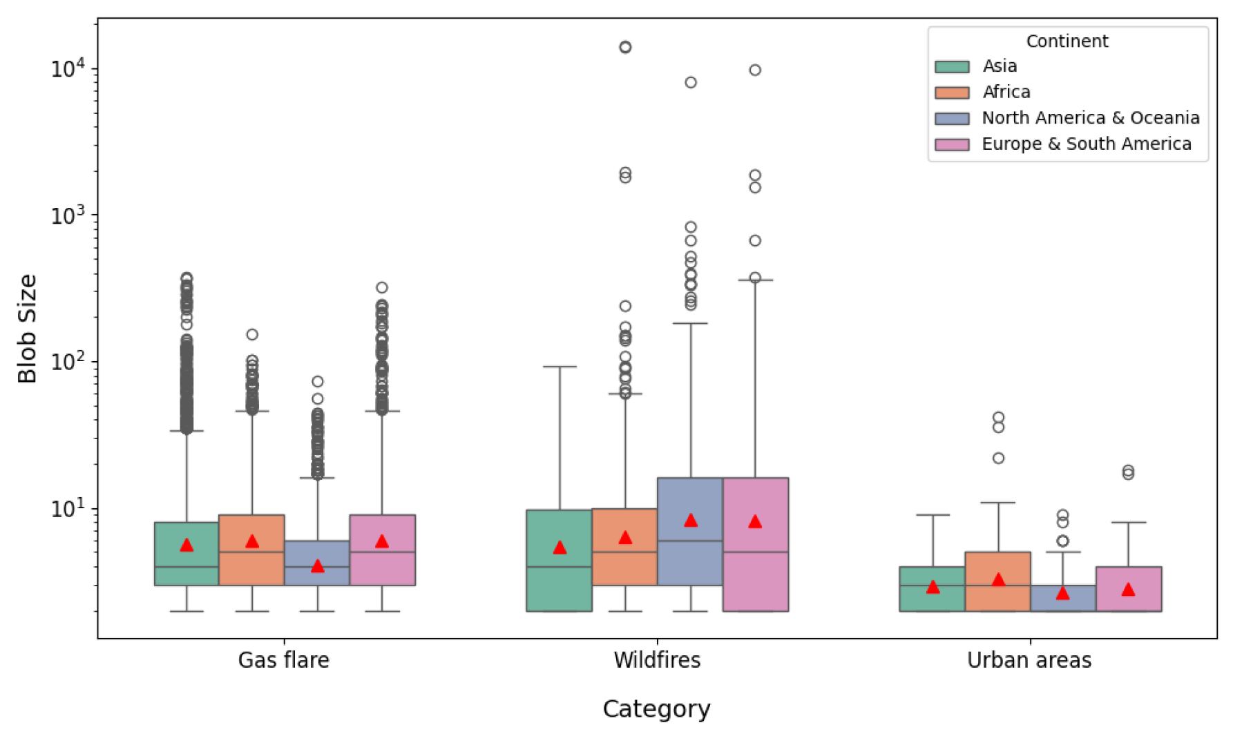
Figure 5.
Best model and band combination results: (a) B7 patch (Fold 4), (b) zoomed mask, (c) U-Net (B2, B6, B7), (d) Att-U-Net (B2, B6, B7), (e) LC U-Net (B4, B5, B6, B7), and (f) Att-LC U-Net (B1–B10).
Figure 5.
Best model and band combination results: (a) B7 patch (Fold 4), (b) zoomed mask, (c) U-Net (B2, B6, B7), (d) Att-U-Net (B2, B6, B7), (e) LC U-Net (B4, B5, B6, B7), and (f) Att-LC U-Net (B1–B10).
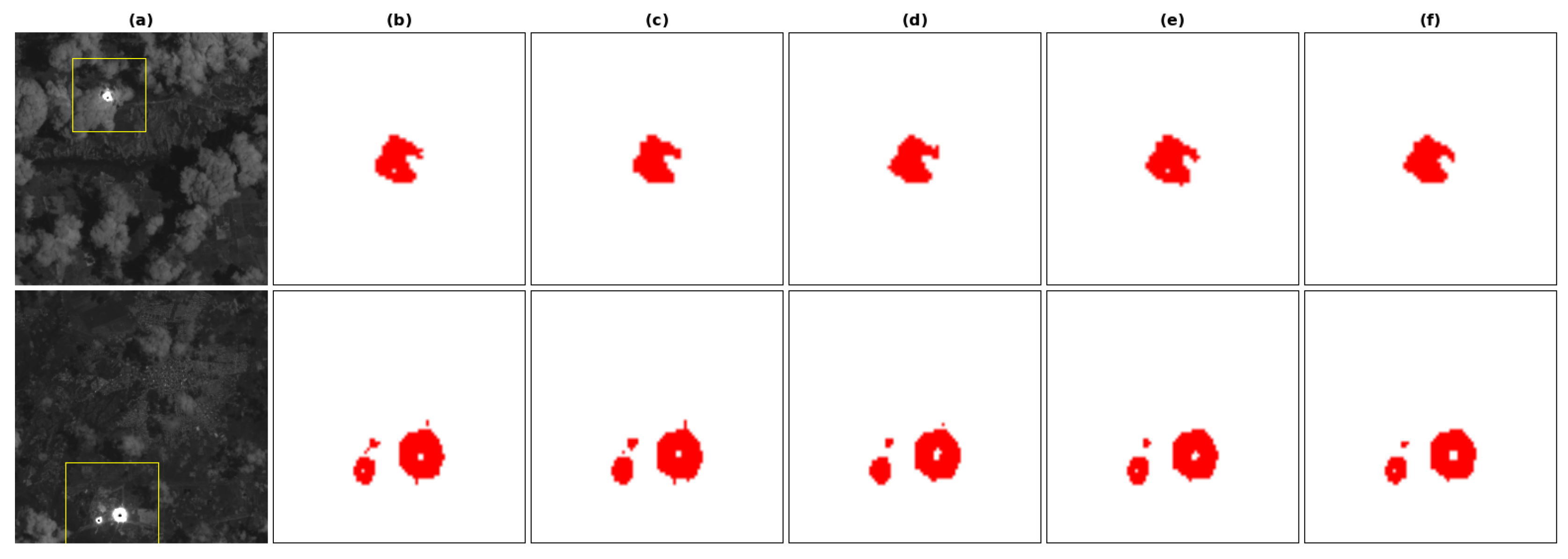
Figure 6.
Wildfire false positives: (a) B7 patch (Fold 3), (b) Active-fire output, (c) U-Net (B2,B6,B7), (d) Att-U-Net (B2,B6,B7), (e) LC U-Net (B4,B5,B6,B7), (f) Att-LC U-Net (B1-B10).
Figure 6.
Wildfire false positives: (a) B7 patch (Fold 3), (b) Active-fire output, (c) U-Net (B2,B6,B7), (d) Att-U-Net (B2,B6,B7), (e) LC U-Net (B4,B5,B6,B7), (f) Att-LC U-Net (B1-B10).
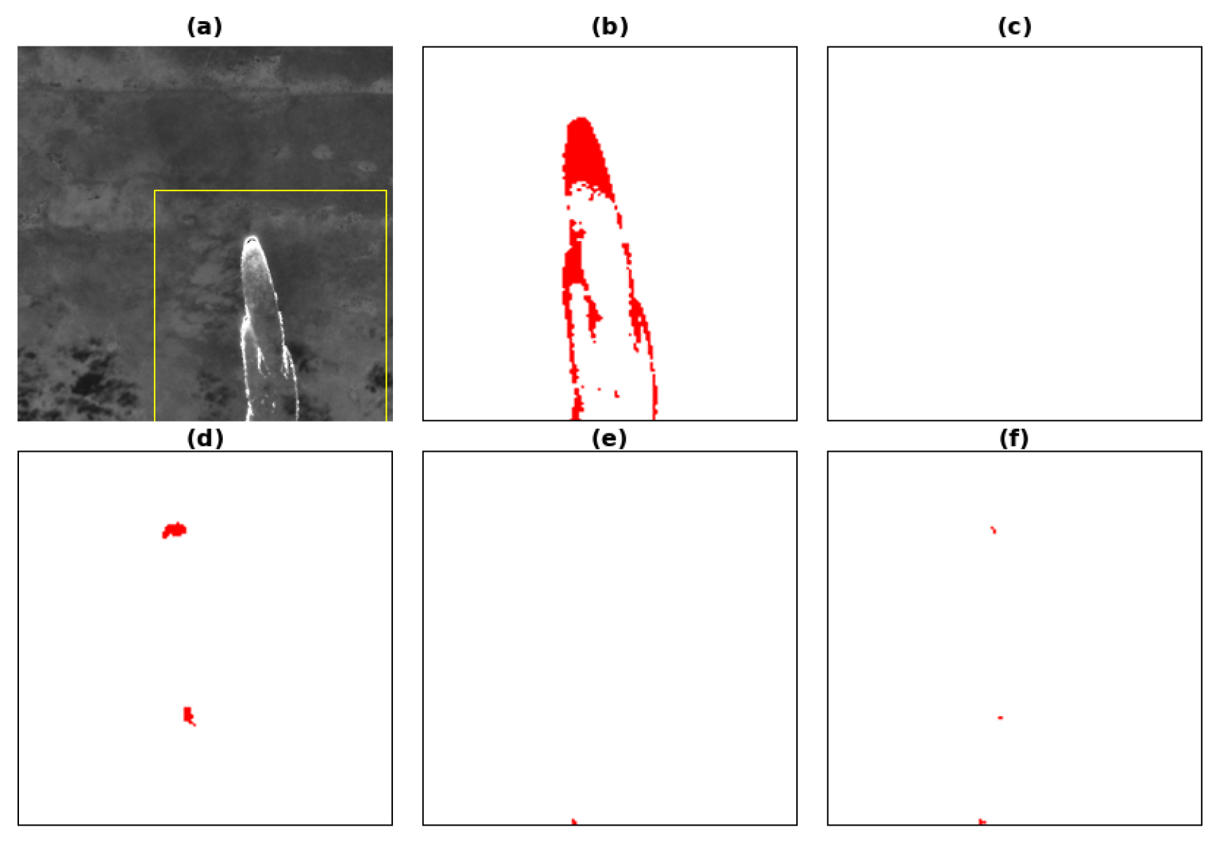
Figure 7.
Urban false positives (Fold 1): (a) B7 patch, (b) Active-fire output, (c) U-Net (B2,B6,B7), (d) Att-U-Net (B2,B6,B7), (e) LC U-Net (B4,B5,B6,B7), (f) Att-LC U-Net (B1-B10).
Figure 7.
Urban false positives (Fold 1): (a) B7 patch, (b) Active-fire output, (c) U-Net (B2,B6,B7), (d) Att-U-Net (B2,B6,B7), (e) LC U-Net (B4,B5,B6,B7), (f) Att-LC U-Net (B1-B10).
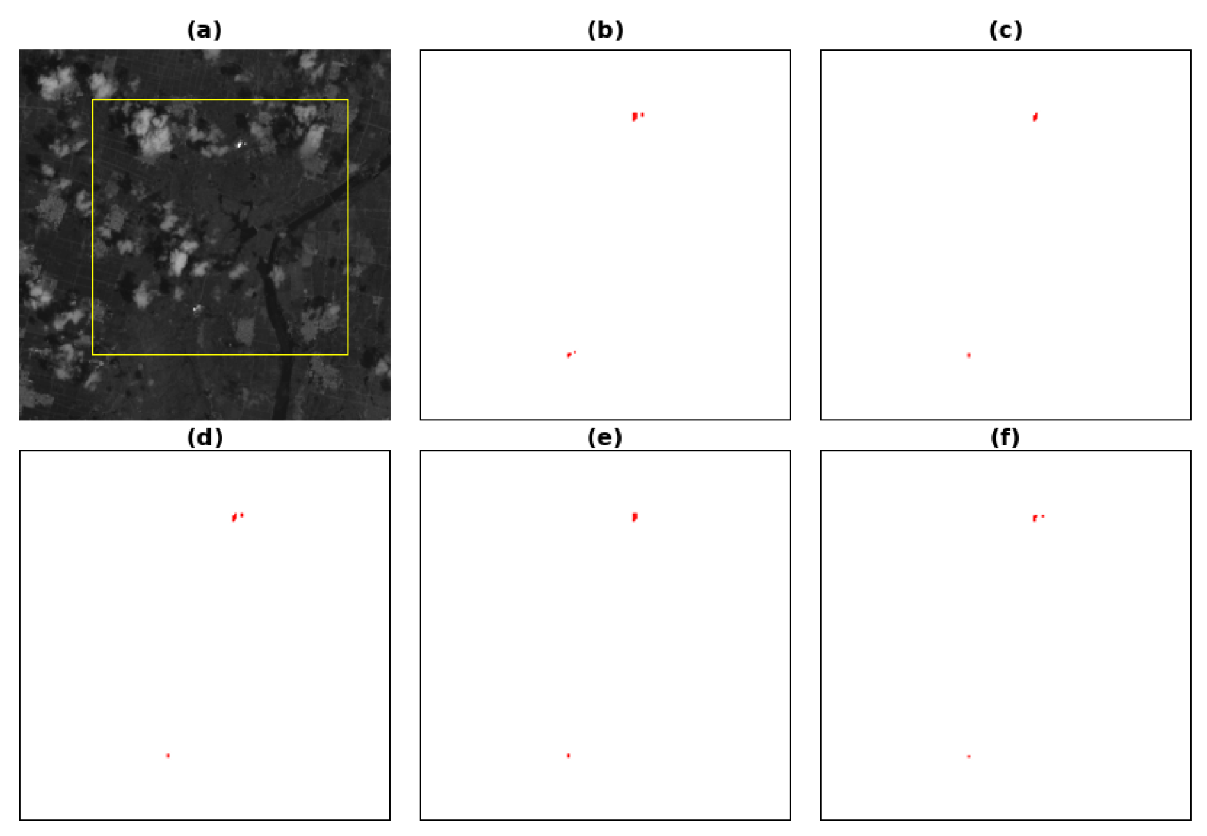

Table 1.
Number of patches / pixels per fold, considering the flare, wildfire and highly reflective urban categories.
Table 1.
Number of patches / pixels per fold, considering the flare, wildfire and highly reflective urban categories.
| Fold | Flare | Non-flare | |
|---|---|---|---|
| Wildfire | Urban | ||
| (1) | 2,990 / 44,725 | 67 / 1,275 | 66 / 331 |
| (2) | 1,757 / 19,871 | 66 / 36,297 | 66 / 634 |
| (3) | 1,261 / 9,506 | 66 / 17,293 | 66 / 329 |
| (4) | 1,329 / 17,717 | 66 / 19,505 | 65 / 409 |
Table 2.
F1 scores for the continent-based K-Fold split (1: Asia, 2: Africa, 3: North America & Oceania, 4: Europe & South America). Reported metrics include mean F1, standard deviation, mean precision, recall, and IoU across all folds. All patches are included, encompassing flares as well as false positives from wildfires and urban areas.
| Model | Bands | F1 per Fold | F1 Mean ± Std | Mean Metrics | |||||
|---|---|---|---|---|---|---|---|---|---|
| (1) | (2) | (3) | (4) | (P) | (R) | (IoU) | |||
| U-Net | 2,6,7 | 0.95 | 0.94 | 0.92 | 0.94 | 0.94 ± 0.01 | 0.93 | 0.94 | 0.88 |
| U-Net | 5,6,7 | 0.93 | 0.94 | 0.64 | 0.91 | 0.86 ± 0.14 | 0.83 | 0.83 | 0.77 |
| U-Net | 4,5,6,7 | 0.95 | 0.94 | 0.90 | 0.90 | 0.92 ± 0.02 | 0.92 | 0.93 | 0.86 |
| U-Net | 1-10 | 0.89 | 0.92 | 0.86 | 0.92 | 0.90 ± 0.03 | 0.89 | 0.91 | 0.81 |
| Att-U-Net | 2,6,7 | 0.95 | 0.95 | 0.93 | 0.91 | 0.93 ± 0.02 | 0.92 | 0.94 | 0.88 |
| Att-U-Net | 5,6,7 | 0.93 | 0.94 | 0.93 | 0.91 | 0.93 ± 0.01 | 0.93 | 0.93 | 0.86 |
| Att-U-Net | 4,5,6,7 | 0.94 | 0.93 | 0.91 | 0.89 | 0.92 ± 0.02 | 0.92 | 0.92 | 0.85 |
| Att-U-Net | 1-10 | 0.95 | 0.94 | 0.93 | 0.91 | 0.93 ± 0.02 | 0.93 | 0.93 | 0.87 |
| LC U-Net | 2,6,7 | 0.95 | 0.93 | 0.71 | 0.70 | 0.82 ± 0.14 | 0.75 | 0.94 | 0.72 |
| LC U-Net | 5,6,7 | 0.94 | 0.93 | 0.83 | 0.90 | 0.90 ± 0.05 | 0.89 | 0.92 | 0.82 |
| LC U-Net | 4,5,6,7 | 0.94 | 0.93 | 0.91 | 0.91 | 0.92 ± 0.01 | 0.94 | 0.91 | 0.86 |
| LC U-Net | 1-10 | 0.94 | 0.78 | 0.89 | 0.92 | 0.88 ± 0.07 | 0.84 | 0.94 | 0.80 |
| Att-LC U-Net | 2,6,7 | 0.93 | 0.94 | 0.68 | 0.86 | 0.85 ± 0.12 | 0.81 | 0.93 | 0.76 |
| Att-LC U-Net | 5,6,7 | 0.93 | 0.88 | 0.63 | 0.88 | 0.83 ± 0.14 | 0.78 | 0.92 | 0.72 |
| Att-LC U-Net | 4,5,6,7 | 0.92 | 0.90 | 0.89 | 0.85 | 0.89 ± 0.03 | 0.89 | 0.89 | 0.80 |
| Att-LC U-Net | 1-10 | 0.93 | 0.91 | 0.88 | 0.90 | 0.90 ± 0.02 | 0.90 | 0.91 | 0.83 |
Table 3.
FPR by class and model across folds: (1) Asia, (2) Africa, (3) North America & Oceania, (4) South America & Europe.
Table 3.
FPR by class and model across folds: (1) Asia, (2) Africa, (3) North America & Oceania, (4) South America & Europe.
| Model | Bands | Fold 1 | Fold 2 | Fold 3 | Fold 4 | ||||
|---|---|---|---|---|---|---|---|---|---|
| Wildfire | Urban | Wildfire | Urban | Wildfire | Urban | Wildfire | Urban | ||
| U-Net | 2,6,7 | 0.082 | 0.386 | 0.006 | 0.292 | 0.008 | 0.213 | 0.009 | 0.117 |
| Att-U-Net | 2,6,7 | 0.156 | 0.351 | 0.005 | 0.224 | 0.018 | 0.264 | 0.046 | 0.179 |
| LC U-Net | 4,5,6,7 | 0.165 | 0.302 | 0.006 | 0.116 | 0.012 | 0.224 | 0.002 | 0.162 |
| Att-LC U-Net | 1-10 | 0.322 | 0.426 | 0.031 | 0.170 | 0.052 | 0.118 | 0.003 | 0.351 |
Disclaimer/Publisher’s Note: The statements, opinions and data contained in all publications are solely those of the individual author(s) and contributor(s) and not of MDPI and/or the editor(s). MDPI and/or the editor(s) disclaim responsibility for any injury to people or property resulting from any ideas, methods, instructions or products referred to in the content. |
© 2025 by the authors. Licensee MDPI, Basel, Switzerland. This article is an open access article distributed under the terms and conditions of the Creative Commons Attribution (CC BY) license (http://creativecommons.org/licenses/by/4.0/).
Copyright: This open access article is published under a Creative Commons CC BY 4.0 license, which permit the free download, distribution, and reuse, provided that the author and preprint are cited in any reuse.


