
Submitted:
20 November 2025
Posted:
24 November 2025
You are already at the latest version
Abstract
In parametric statistical analysis, the independent-samples t-test is a widely used method for comparing the means of two different groups. Under the assumption of homogeneity of variances and normally distributed data, it evaluates the statistical significance of observed differences between group means. The fundamental ideas of the independent-samples t-test—including its assumptions, hypotheses, effect size considerations, and methodological applications in research—are investigated in this review. Furthermore, fundamental methodological issues, including the interpretation of statistical significance, are covered. Aiming to increase researchers' competency in using and interpreting the independent-samples t-test across studies, this paper provides a thorough tutorial on the test. In addition, this review highlights JASP (Jeffrey’s Amazing Statistics Program), an open-source statistical platform with an interface for conducting independent-samples t-tests. JASP provides automated assumption checks, effect size calculations, and graphical outputs, making it accessible for researchers with varying levels of statistical expertise.
Keywords:
Independent-samples t-test
; JASP
; Parametric analysis
; Assumptions
; Effect size
; Statistical interpretation
; Research methodology
1. Introduction
The parametric independent-samples t-test assesses whether the population means of two groups are equal or differ, based on independent observations [1]. The test requires a continuous (interval/ratio) dependent variable (DV) and an independent variable (I_DV) coded as a nominal variable with two groups (dichotomous).
The independent-samples t-test is suitable when the observations within each group are independent, either through random sampling or random assignment, and when the DV is measured on a continuous scale (e.g., ratio or interval measurement). When testing for group mean differences, a t-test can be the procedure of choice under two additional assumptions: the DV is approximately normally distributed within the groups, and the variances of the I_DVs are equal across groups. When violations of these conditions must be tolerated, the statistical analysis can still yield reasonable results when certain precautions are employed [2].
The t statistic is defined as t = (M1 – M2) / SE, where M1 and M2 are the sample means of groups 1 and 2, respectively, and SE is the standard error of the difference between the two groups. The standard error can be calculated based on either a pooled estimate of the common population variance (homogeneity of variance assumed) or a separate estimate based on each sample variance alone (homogeneity of variance not assumed) [3]. A large t-score indicates a greater difference between groups. The smaller the t-score, the greater the similarity between groups. A t-score of 5 means that the groups are five times as different from each other as they are within each other.
Table 1 summarises the primary purpose, common alternative names, and practical examples of the independent-samples t-test across different research fields.
This review outlines the application of the independent samples t-test using the open-source software JASP, Version 0.95.3.0 [7]. The software supports multiple statistical modules, including the “T-Tests” Toolkit, which implements the independent-samples t-test [8]. The output reports the population mean scores and variances of the two groups examined, the test statistic, degrees of freedom, and associated p-value, as well as Levene’s Test for Equality of Variances and confidence intervals for the mean difference.
2. Fundamentals of the Independent-Samples t-Test
2.1. Studying the Difference Between Two Independent Groups
When measuring a DV across two independent groups and aiming to compare them, one can calculate the DV mean within each group and use an independent-samples t-test to compare the groups. This process involves subtracting the mean DV of one group from the other, yielding the difference between the two group means. It is essential to recognise that the participants constituting these groups are typically samples drawn from substantially larger populations. Our primary interest lies in these populations rather than in the specific sample members. Due to sampling variability, the group means and their differences will vary across different samples recruited for a study. Therefore, the independent-samples t-test evaluates whether the population means of the groups differ, rather than merely assessing differences in sample means [9,10,11].
2.2. Null and Alternative Hypotheses
The null hypothesis (Ho) posits that the population means of the two independent groups are equal.
The independent-samples t-test is frequently configured to address a specific null and alternative hypothesis. The null hypothesis for an independent-samples t-test is:
H0: the population means of the two groups are equal (i.e. µ1 = µ2) or H0: the difference between the population means is zero (i.e. µ1 – µ2 = 0).
And the alternative hypothesis is:
HA: the population means of the two groups are not equal (i.e. µ1 ≠ µ2) or HA: the difference between the population means is not zero (i.e
An independent-samples t-test calculates a significance level (p-value), which signifies the probability that the observed difference between the sample group means is as extreme as the one observed, assuming the null hypothesis holds true [12,13]. Typically, if this probability is sufficiently small (e.g., p < 0.05), it is inferred that the two-population means are unlikely to be equal, thereby supporting the alternative hypothesis and leading to the rejection of the null hypothesis. Conversely, if the p-value exceeds this threshold (often p > 0.05), the evidence is not sufficient to reject the null hypothesis. It is important to emphasise that the acceptance of the null hypothesis is not appropriate. Furthermore, hypothesis tests pertain to population means rather than sample means [14,15].
2.3. Effect Sizes
The independent-samples t-test, utilised as a null-hypothesis significance test, offers insights into whether the differences between group means are statistically significant (i.e., indicative of differences within the population); however, it does not specify the magnitude of these differences. To mitigate this limitation, an effect size can be calculated. Various types of effect size exist, each aiming to quantify the significance of the results through different methodologies [16].
In this guide, we will demonstrate how to calculate the effect size measure d, which is a type of effect size that evaluates the significance of the I_DV by expressing the difference between the group means as a ratio of the standard error of the mean difference.
2.4. Sample Size and (un)Balanced Designs
As a general guideline, our study should include six or more participants per group to proceed with an independent-samples t-test; however, it is preferable to have a larger sample size. Although an independent-samples t-test can be conducted with fewer than six participants, our capacity to infer or generalise the findings to a broader population becomes more limited [17,18].
An equal number of participants in each group characterises a balanced design. Conversely, an unbalanced design occurs when the sample sizes across groups differ. Generally, a greater imbalance in the design amplifies the adverse impact of assumption violations on the test's validity. Ideally, a balanced design is preferable, though it may be challenging to achieve in practical settings [17,18].
3. Study Designs
An independent-samples t-test is most often used to analyse results from three different study designs, as shown in Table 2.
4. Methodological Steps
Carrying out an independent-samples t-test can be a simple, five-step process (Table 3). However, sometimes we have to make adjustments to account for the nature of the data we are analysing.
5. Data Setup and Example
5.1. Example Used in This Guide
A pharmaceutical company has been commissioned to develop a social media advertisement aimed at promoting a new cosmetic product. Given that the product is intended for both men and women, the advertisement must be equally appealing to both genders. The company seeks to determine whether men and women engage with the advertisement in a similar manner. To this end, the advertisement is presented to a sample of twenty men and twenty women, who are subsequently asked to complete a questionnaire designed to measure their level of engagement with the advertisement. The questionnaire yields an overall engagement score.
This overall engagement score serves as the dependent variable (DV), which has been designated as' engagement' within the JASP statistical software. The independent variable (iv), labelled as' gender' in JASP, comprises two groups: "Male" and "Female. " The advertising agency is interested in examining whether the independent variable (gender) influences the dependent variable (engagement), and whether there are statistically significant differences in engagement levels between the two gender groups. In other words, the agency wishes to ascertain if the mean engagement scores differ between males and females. As the agency desires the advertisement to be equally engaging across genders, they hypothesise that there will be no significant difference in engagement scores.
5.2. Setting Up the Data
For an independent-samples t-test, we will have two variables. In this example, these are (Figure 1):
1) The DV, engagement, which is the overall engagement score from the questionnaire.
2) The I_DV, gender, which has two groups: "Male" and "Female".
The figure shows two variables: one in each column. The I_DV is gender, and the continuous DV is the engagement.
5.3. Null and Alternative Hypotheses
The null hypothesis for this example is:
H0: µmale = µfemale
Where µ = population mean and subscripts = the names of the different levels of the I_DV: "Male" and "Female". This indicates that the mean engagement scores for males and females are equal within the population.
The alternative hypothesis is:
HA: µmale ≠ µfemale
This states that the mean engagement scores for males and females differ in the population.
This guide discusses how to provide evidence to accept or reject the alternative hypothesis and reject or fail to reject the null hypothesis.
6. Assumptions and Prerequisites
To conduct an independent-samples t-test, six assumptions must be considered (see Table 4). The initial three assumptions pertain to the selection of study design and the measurements employed, whereas the remaining three assumptions concern the characteristics of the data collected.
Normality, homogeneity of variances, and independence of observations are often considered vital prerequisites for computing t-test results for independent samples reliably. However, it is essential to note that the test is relatively robust to deviations from the normality assumption, particularly when sample sizes are moderate to large [23,24]. The assumption of identical variance plays a more critical role in the statistical process; when this assumption is violated, it can lead to bias in the R estimate, inflate Type I error rates, and ultimately compromise the overall validity of the statistical inference being drawn. (MacLehose et al.2021)(Knief & Forstmeier, 2021) Nevertheless, the t-test remains robust to violations of the homogeneity-of-variance assumption, especially when group sample sizes are balanced. This gives researchers a degree of flexibility when applying the test under less-than-ideal conditions [1,25].
To conduct an independent-samples t-test, six assumptions must be acknowledged (see Table 2). The initial three assumptions pertain to the study design and the measurements selected, while the subsequent three assumptions concern the properties of the collected data.
The remaining three assumptions pertain to the characteristics of our data and can be evaluated using JASP Statistics. Given that it is not unusual for the collected data to breach (i.e., fail to meet) one or more of these assumptions, we propose various approaches for proceeding. These include (a) implementing adjustments to the data to ensure compliance with the assumptions, (b) employing an alternative statistical test, or (c) continuing with the analysis despite the violation of certain assumptions [26].
The assumption of homogeneity of variances posits that the population variances for each group in the independent dependent variable (I_DV) are equal. When sample sizes across groups are similar, violating this assumption generally poses minimal concern. However, in cases where sample sizes are markedly different, the independent-samples t-test becomes sensitive to such violations. To address this, JASP employs Levene's test for equality of variances and performs two variations of the independent-samples t-test: one using pooled variances for situations where the assumption holds, and another utilising separate variances with the Welch-Satterthwaite correction, which is appropriate when the assumption is violated. This approach ensures that the Results remain valid regardless of whether the assumption of equal variances is met.
It is necessary to examine the boxplot to identify any potential outliers within each group. Data points exceeding 1.5 box-lengths from the edge of their respective box are designated as outliers by JASP and are represented as circular dots. Data points that are more than 3 box-lengths from the box edge are classified as extreme points, also known as extreme outliers. Both categories of outliers are annotated with their case number, which corresponds to their row number in the Data View window, to facilitate identification.
Transformations are usually not warranted unless the data are not normally distributed, so we might consider this option only if we also need to apply a transformation due to non-normality [30]. Additionally, it is important to recognise the disadvantage of complicating the interpretation of the independent-samples t-test, as the original data values are no longer utilised. Should this approach be selected, it becomes necessary to re-conduct all the assumption tests previously performed.
The Shapiro-Wilk test is recommended in scenarios involving small sample sizes (less than 50 participants) and when confidence in the visual interpretation of Normal Q-Q plots or other graphical normality tests is limited. This test evaluates whether the data within each category of the independent dependent variable (I_DV) adhere to a normal distribution.
When the data are normally distributed- that is, the assumption of normality is satisfied- the significance level should exceed 0.05 (p > 0.05). For larger sample sizes exceeding 50, the employment of graphical methods, such as a Normal Q-Q plot, is advisable. This recommendation arises from the fact that the Shapiro-Wilk test tends to identify even minor deviations from normality as statistically significant (indicating non-normal distribution) when sample sizes are substantial.
The assumption of homogeneity of variances posits that the population variances across the groups defined by the I_DV are equal. If the sample sizes in each group are comparable, violations of this assumption are generally not of great concern. Nevertheless, when there are significant discrepancies in sample sizes, the independent-samples t-test becomes sensitive to such violations. .
7. Running the Test
We need to check the distribution and boxplots in Descriptives to assess the distribution and identify outliers visually. Then, we need to go to T-Tests > Independent Samples t-test, enter the scale DV in the Dependent Variable box and I_DV in the Grouping Variable box (Figure 2). In the analysis window, we have to tick certain options, as shown in Figure 2.
8. Interpreting the Output
After running the independent-samples t-test procedure, JASP will generate tables containing all the information we need to report the results.
8.1. Descriptive Statistics
After clicking Descriptives box, JASP will generate a Group Descriptives table containing some useful descriptive statistics for the two groups (Figure 3).
The columns of the table have the following meaning: N: Number of cases (e.g., participants); Mean: Mean/average; SD: Standard deviation of the sample; SE: Standard error of the mean.
Each row in the table above presents statistics on the DV (engagement) for the different categories of the I_DV (gender).
The group descriptives table serves to elucidate specific aspects of the data, such as whether there is an equal number of participants in each group (the "N" column), which group exhibits a higher or lower mean score (the "Mean" column), and the implications of this for the results. Additionally, it assesses whether the variation within each group is comparable (e.g., the "SD" column). In this instance, it is evident that the groups' sizes were equal (n = 20), with males demonstrating a higher mean engagement score (5.5589) compared to females (5.2999), albeit with a lower standard deviation (0.29190 versus 0.39339), indicating that female scores exhibited greater variability than those of males. These descriptive statistics, specifically the mean (" Mean " column) and standard deviation (" SD " column), will be presented in the results section. It is important to note that, despite both the standard deviation and the standard error of the mean being utilised to describe data, the latter is often considered inappropriate in many contexts where it is presented.
With an initial understanding of the data gleaned from these descriptive statistics, it becomes necessary to evaluate the magnitude of the mean difference between groups and to determine its statistical significance. Prior to this, however, it is essential to examine the assumption of equal variances, ensuring the accurate reporting of the independent-samples t-test results. ly.
8.2. Assumption of Homogeneity of Variances
An essential assumption of the independent-samples t-test is that the variances of the two groups are equal within the population. Failure to satisfy this assumption- specifically, if the variances are unequal- will increase the likelihood of committing a Type I error. The equality of variances is commonly referred to as homogeneity of variances. Consequently, it is desirable for the variance of the dependent variable (DV) to be equivalent across the two groups of I_DV.
In this example, utilising the Descriptives icon (with data not shown), it is observed that the variance for males is 0.085, whereas for females, it is 0.155- indicating that females exhibit nearly twice the variability in engagement scores compared to males. Nonetheless, these estimates are derived from the two samples within this study, and variances are subject to change due to sampling variability. To formally evaluate whether these variances differ within the population, JASP employs Levene's Test for Equality of Variances. In essence, Levene's test assesses whether the two samples originate from populations with identical variances. The results of this test are presented in part D of Figure 3.
To determine whether the population variances are equal, one must refer to the "p" value located in the column under " Test of Equality of Variances. " In this case, the significance value is 0.186, indicating that the assumption of homogeneity of variances has been satisfied. Conversely, if the p-value is less than 0.05, this indicates that the population variances are unequal, thus violating the assumption. In this example, the variances of engagement scores in both groups are deemed equal, and therefore, the assumption of homogeneity of variances is upheld.
Levene's test for equality of variances tests the null hypothesis that the population variances are equal, or, more formally, that the two samples are drawn from populations with the same variance. This can be expressed as:
H0: σ12 = σ22
Where σ = population standard deviation (remembering that variance is standard deviation squared), the subscripts 1 and 2 represent the two independent groups. The alternative hypothesis of this test is that the population variances are not equal. Again, this can be formally written as:
HA: σ12 ≠ σ22
Levene's test operates in the same way as most inferential statistical tests. In this case, it calculates an F-statistic under an F-distribution, with the p-value indicating the evidence against the null hypothesis. Therefore, a statistically significant result means that we should accept the alternative hypothesis: that the population variances are unequal.
If the assumption of homogeneity of variances is violated, this is sometimes referred to as heteroscedasticity, meaning unequal variances.
The standard independent-samples t-test assumes homogeneity of variances. If it is not met, the result might not be valid. However, a modification to the standard t-test can accommodate unequal variances and still yield a valid test result. This modified t-test is often called the unequal-variance t-test, the separate-variances t-test, or the Welch t-test after its creator [31]. It is an approximate answer to the Behrens–Fisher problem, which, in this case, is determining the probable difference between two means when the population variances are unequal. JASP will generate the results from both types of t-tests – standard and Welch – in the output when we click Welch, as shown in Figure 4.
As previously stated, if the assumption of normality or the presence of outliers in the data has been violated, alternative methods such as the Mann-Whitney U test may be considered in place of the independent-samples t-test. The Mann-Whitney U test compares the differences between group medians, provided that the shape and dispersion of the dependent variable scores are similar across both groups. Additionally, if Levene's test indicates unequal variances, the appropriateness of interpreting the Mann-Whitney U test as a test of median differences may be compromised.
When we have an unbalanced design (i.e., unequal group sizes), and the differences in sample size are not unsubstantial, it is recommended to use the Welch t-test.
8.3. Mean Difference Between Groups
To determine the mean difference between the two groups and provide a measure of the likely range (plausible values) of this mean difference, we need to consult the last four columns of the Independent Samples Test.
We have established that the mean engagement score for males (5.559 ± 0.292) was higher than that for females (5.300 ± 0.393). The mean difference between the two group means is presented in the "Mean Difference" column and is 0.259 (Figure 5). This mean difference is calculated as the difference between the mean engagement score for males and for females, i.e., 5.559 – 5.300 = 0.259. However, we would also like to report a measure of variability of the mean difference, which we can do with the SE difference (the "SE Difference" column), which is 0.110, or using 95% confidence intervals (the "Lower" and "Upper" columns), which are 0.037 to 0.481. We prefer to report 95% confidence intervals, but either is fine (unlike when reporting descriptive statistics, with sampling distributions, it is fine to use the standard error).
‘Statistic’ indicates we are comparing it to a t-distribution (t-test). The ‘df’ indicates the degrees of freedom, which is N – 2. 2.365 indicates the obtained value of the t-statistic (obtained t-value). If the null hypothesis is correct, the ‘p’ indicates the probability of obtaining the observed t-value.
9. Reporting
When we report the results, we can focus on the main findings, but it is good practice to report the results of the assumption tests we conducted as well. In this section, we explain how to report the findings when the assumption of homogeneity of variances was met and when it was violated. Table 4 shows how to report the main findings in a step-wise approach.
9.1. Reporting Statistical Significance
To ascertain the statistical significance of the independent-samples t-test, it is essential to consult the Independent Samples Test table (refer to Figure 5). This table provides the observed t-value (located in the "Statistic" column), the degrees of freedom (denoted in the "df" column), and the p-value indicating statistical significance (found in the "p" column). A p-value less than 0.05 signifies that the difference in means between the two groups is statistically significant. Conversely, a p-value greater than 0.05 indicates no statistically significant difference in the group means. In the present example, the p-value is 0.023 (i.e., p < 0.05). Consequently, it can be concluded that there are statistically significant differences in mean engagement scores between males and females. Alternatively expressed, the difference in mean engagement scores between the two groups is statistically significant. This outcome implies that the probability of obtaining a mean difference as large as the observed one, assuming the null hypothesis is true, is approximately 2.3%. As previously stated, the independent-samples t-test evaluates whether the population means are equal.
In addition to reporting the statistical significance value, JASP also reports t = 2.365 (the "Statistic" column) and 38 degrees of freedom (the "df" column). n).
9.2. Reporting the Null and Alternative Hypotheses
Occasionally, it may be required to state the null and alternative hypotheses for the independent-samples t-test based on the data, and to determine whether to reject the null hypothesis and accept the alternative hypothesis, or to fail to reject both hypotheses. It is important to note that the null hypothesis cannot be accepted definitively; therefore, it is never stated as such.
In the event that the independent-samples t-test yields a statistically significant result (p < 0.05), it indicates that the likelihood of the observed mean difference between the two groups occurring by chance—assuming the null hypothesis is true—is less than 5 in 100. The null hypothesis posits that the population means of the two groups are equal. Consequently, we reject the null hypothesis and accept the alternative hypothesis, which asserts that the population means are not equal. Conversely, if the test results are not statistically significant (p > 0.05), we must reject the alternative hypothesis and fail to reject the null hypothesis.
9.3. Calculating and Reporting an Effect Size
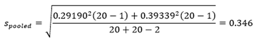
Effect sizes are increasingly used to convey results; however, they remain considerably less prevalent than reporting statistical significance. To determine this effect size, one must divide the mean difference between the groups by the pooled standard deviation, then take the square root, as illustrated below.
Where || means the absolute value (negative value becomes a positive value) and,
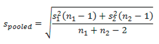
So,
And therefore,
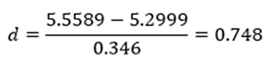
An effect size is an attempt to measure the practical significance of the result. The importance of the value of Cohen's d (as reported by Cohen (1988)) [32] (Table 5).
Given the effect size d = 0.748, we infer there is a moderate effect. It is recommended to report the effect size alongside the results of the hypothesis test, specifically the independent-samples t-test. It is important to note that the above calculation is valid only when variances are homogeneous, since it employs the pooled variance. Additionally, a significant limitation of utilising effect sizes is that the guidelines for their importance are often specific to the context, and as of now, comprehensive guidelines for interpreting the magnitude of an effect size are lacking. Furthermore, there are typically multiple measures of effect size, such as various effect sizes, as illustrated in Figure 6.
10. Practical vs. Statistical Significance
Although a statistically significant difference was observed between males and females in their engagement scores, the institution may conclude that the mean difference of 0.26 holds limited practical significance. The mere presence of statistical significance does not inherently imply practical importance. Statistical significance solely signifies that the result is unlikely to be attributable to sampling error; while this is meaningful, it does not convey the strength of the differences. In this context, confidence intervals (CIs) are instrumental, as they offer not only the majority of information pertaining to the statistical test but also insights into the magnitude of the observed difference.
11. Graphing the Output
Suppose that the groups of the independent dependent variable (IDV) are not derived from an underlying continuous scale, such as gender. In such cases, a bar chart or line graph is suitable to accompany the results of an independent-sample t-test. For instance, error bars should be incorporated in simple bar or line charts to depict standard deviations or 95% confidence intervals.
Conversely, if the groups are based on an underlying continuous scale, such as age groups (< 45 years and ≥ 45 years), it is preferable to present the data graphically in a manner similar to a histogram. This can be achieved by increasing the width of the columns in a bar chart.
An example of a simple bar chart illustrating the results, as shown in Figure 7, includes 95% confidence intervals but lacks additional formatting for aesthetic enhancement.
12. Conclusion
The steps outlined provide a rigorous approach to implementing an independent-samples t-test in JASP to test for significant mean differences between two groups, assuming specific conditions are met. It remains to emphasise the critical amplification of these sound methodologies through the adoption of user-friendly software, an opportunity offered by JASP. This work has validated JASP’s capacity to perform the independent-samples t-test in a manner that is transparent, reproducible, and integral to studies of comparable characteristics or datasets, while adhering to APA standards and contemporary recommendations on statistical analyses. Parameters recorded at this stage continue to fulfil requirements for later use in specifying further approaches or tests.
While statistical significance is important, researchers also have to consider how their findings might be practically relevant. When assumptions are violated, nonparametric techniques, such as the Mann-Whitney U test, should be considered. This work underscores the need to perform and assess the independent-samples t-test precisely to ensure that statistical analyses adequately support evidence-based decision-making across diverse research domains.
References
- Kim, T.K. T Test as a Parametric Statistic. Korean journal of anesthesiology 2015, 68, 540–546. [CrossRef]
- Berkes, P.; Fiser, J. A Frequentist Two-Sample Test Based on Bayesian Model Selection. arXiv preprint arXiv:1104.2826 2011.
- Alsuof, E.A.; Alsayed, A.R.; Zraikat, M.S.; Khader, H.A.; Hasoun, L.Z.; Zihlif, M.; Ata, O.A.; Zihlif, M.A.; Abu-Samak, M.; Al Maqbali, M. Molecular Detection of Antibiotic Resistance Genes Using Respiratory Sample from Pneumonia Patients. Antibiotics 2025, 14, 502. [CrossRef]
- Alsayed, A.R.; Hasoun, L.; Al-Dulaimi, A.; AbuAwad, A.; Basheti, I.; Khader, H.A.; Al Maqbali, M. Evaluation of the Effectiveness of Educational Medical Informatics Tutorial on Improving Pharmacy Students’ Knowledge and Skills about the Clinical Problem-Solving Process. Pharmacy Practice 2022, 20, 2652.
- Alimam, S.M.; Alhmoud, J.F.; Khader, H.A.; Alsayed, A.R.; Abusamak, M.; Mohammad, B.A.; Mosleh, I.; Khadra, K.A.; Aljaberi, A.; Habash, M. Effect of Weekly High-Dose Vitamin D3 Supplementation on the Association between Circulatory FGF-23 and A1c Levels in People with Vitamin D Deficiency: A Randomized Controlled 10-Week Follow-up Trial. Pharmacy Practice 2024, 22, 1–8. [CrossRef]
- Al-kilkawi, Z.M.; Basheti, I.A.; Obeidat, N.M.; Saleh, M.R.; Hamadi, S.; Abutayeh, R.; Nassar, R.; Alsayed, A.R. Evaluation of the Association between Inhaler Technique and Adherence in Asthma Control: Cross-Sectional Comparative Analysis Study between Amman and Baghdad. Pharmacy Practice 2024, 22, 1–12.
- Alsayed, A.R. Mastering Descriptive Statistics in JASP: From Data to Decisions for Measures of Central Tendency and Dispersion. 2025.
- Melendez, C. A Monte Carlo Study of Several Different Approaches to the Behrens–Fisher Problem. 2016.
- Al-Rshaidat, M.M.; Al-Sharif, S.; Tamimi, T.A.; Al-Zeer, M.A.; Samhouri, J.; Alsayed, A.R.; Rayyan, Y.M. First Middle Eastern-Based Gut Microbiota Study: Implications for Inflammatory Bowel Disease Microbiota-Based Therapies. Pharmacy Practice 2025, 23, 1–12. [CrossRef]
- Zihlif, M.; Zakaraya, Z.; Feda’Hamdan, A.S.; Tahboub, F.; Qudsi, S.; Abuarab, S.F.; Daghash, R.; Alsayed, A.R. Hepatocyte Nuclear Factor 4, Alpha (HNF4A): A Potential Biomarker for Chronic Hypoxia in MCF7 Breast Cancer Cell Lines. Pharmacy Practice (1886-3655) 2025, 23. [CrossRef]
- Maddeppungeng, N.M.; Syahirah, N.A.; Hidayati, N.; Rahman, F.U.; Mansjur, K.Q.; Rieuwpassa, I.E.; Setiawati, D.; Fadhlullah, M.; Aziz, A.Y.R.; Salsabila, A. Specific Delivery of Metronidazole Using Microparticles and Thermosensitive in Situ Hydrogel for Intrapocket Administration as an Alternative in Periodontitis Treatment. Journal of Biomaterials science, Polymer edition 2024, 35, 1726–1749. [CrossRef]
- Khaled, R.A.; Alhmoud, J.F.; Issa, R.; Khader, H.A.; Mohammad, B.A.; Alsayed, A.R.; Khadra, K.A.; Habash, M.; Aljaberi, A.; Hasoun, L. The Variations of Selected Serum Cytokines Involved in Cytokine Storm after Omega-3 Daily Supplements: A Randomized Clinical Trial in Jordanians with Vitamin D Deficiency. Pharmacy Practice 2024, 22, 1–10.
- AL-awaisheh, R.I.; Alsayed, A.R.; Basheti, I.A. Assessing the Pharmacist’s Role in Counseling Asthmatic Adults Using the Correct Inhaler Technique and Its Effect on Asthma Control, Adherence, and Quality of Life. Patient preference and adherence 2023, 961–972. [CrossRef]
- Nour, A.; Alsayed, A.; Basheti, I. Parents of Asthmatic Children Knowledge of Asthma, Anxiety Level and Quality of Life: Unveiling Important Associations. Pharmacy Practice 2023, 21, 1–10.
- Bader, D.; Abed, A.; Mohammad, B.; Aljaberi, A.; Sundookah, A.; Habash, M. The Effect of Weekly 50,000 IU Vitamin D3 Supplements on the Serum Levels of Selected Cytokines Involved in Cytokine Storm: A Randomized Clinical Trial in Adults with Vitamin D Deficiency. Nutrients. 2023; 15 (5): 1188. [CrossRef]
- Schober, P.; Bossers, S.M.; Schwarte, L.A. Statistical Significance versus Clinical Importance of Observed Effect Sizes: What Do P Values and Confidence Intervals Really Represent? Anesthesia & Analgesia 2018, 126, 1068–1072.
- Yoon, M.; Lai, M.H. Testing Factorial Invariance with Unbalanced Samples. Structural Equation Modeling: A Multidisciplinary Journal 2018, 25, 201–213. [CrossRef]
- De Winter, J.C. Using the Student’s" t"-Test with Extremely Small Sample Sizes. Practical assessment, research & evaluation 2013, 18, n10.
- Daboul, S.M.; Abusamak, M.; Mohammad, B.A.; Alsayed, A.R.; Habash, M.; Mosleh, I.; Al-Shakhshir, S.; Issa, R.; Abu-Samak, M. The Effect of Omega-3 Supplements on the Serum Levels of ACE/ACE2 Ratio as a Potential Key in Cardiovascular Disease: A Randomized Clinical Trial in Participants with Vitamin D Deficiency. Pharmacy Practice 2022, 21, 2761. [CrossRef]
- Al-Rshaidat, M.M.; Al-Sharif, S.; Al Refaei, A.; Shewaikani, N.; Alsayed, A.R.; Rayyan, Y.M. Evaluating the Clinical Application of the Immune Cells’ Ratios and Inflammatory Markers in the Diagnosis of Inflammatory Bowel Disease. Pharmacy Practice 2022, 21, 2755.
- Al Maqbali, M.; Alsayed, A.; Bashayreh, I. Quality of Life and Psychological Impact among Chronic Disease Patients during the COVID-19 Pandemic. Journal of Integrative Nursing 2022, 4, 217–223. [CrossRef]
- Alsayed, A.R.; Al-Dulaimi, A.; Alnatour, D.; Awajan, D.; Alshammari, B. Validation of an Assessment, Medical Problem-Oriented Plan, and Care Plan Tools for Demonstrating the Clinical Pharmacist’s Activities. Saudi Pharmaceutical Journal 2022, 30, 1464–1472. [CrossRef]
- Hernandez, H. Testing for Normality: What Is the Best Method. ForsChem Research Reports 2021, 6, 1–38.
- Ntumi, S. Reporting and Interpreting Multivariate Analysis of Variance (MANOVA): Adopting the Best Practices in Educational Research. Journal of Research in Educational Sciences (JRES) 2021, 12, 48–57. [CrossRef]
- Nordstokke, D.W.; Colp, S.M. A Note on the Assumption of Identical Distributions for Nonparametric Tests of Location. Practical Assessment, Research & Evaluation 2018, 23, n3.
- Shatz, I. Assumption-Checking Rather than (Just) Testing: The Importance of Visualization and Effect Size in Statistical Diagnostics. Behavior Research Methods 2024, 56, 826–845. [CrossRef]
- Khader, H.; Alsayed, A.; Hasoun, L.Z.; Alnatour, D.; Awajan, D.; Alhosanie, T.N.; Samara, A. Pharmaceutical Care and Telemedicine during COVID-19: A Cross-Sectional Study Based on Pharmacy Students, Pharmacists, and Physicians in Jordan. Pharmacia 2022, 69, 891–901.
- Al-Shajlawi, M.; Alsayed, A.R.; Abazid, H.; Awajan, D.; Al-Imam, A.; Basheti, I. Using Laboratory Parameters as Predictors for the Severity and Mortality of COVID-19 in Hospitalized Patients. Pharmacy Practice 2022, 20, 1–9. [CrossRef]
- Khader, H.; Hasoun, L.Z.; Alsayed, A.; Abu-Samak, M. Potentially Inappropriate Medications Use and Its Associated Factors among Geriatric Patients: A Cross-Sectional Study Based on 2019 Beers Criteria. Pharmacia 2021, 68, 789–795. [CrossRef]
- Alsayed, A.R. Mastering Descriptive Statistics in JASP: From Data to Decisions for Measures of Central Tendency and Dispersion. 2025.
- Welch, B.L. The Generalization of ‘STUDENT’S’Problem When Several Different Population Varlances Are Involved. Biometrika 1947, 34, 28–35.
- Cohen, J. A Power Primer. 2016.
Figure 1.
Variable Configuration and Data Preview for I_DV and DV in JASP.
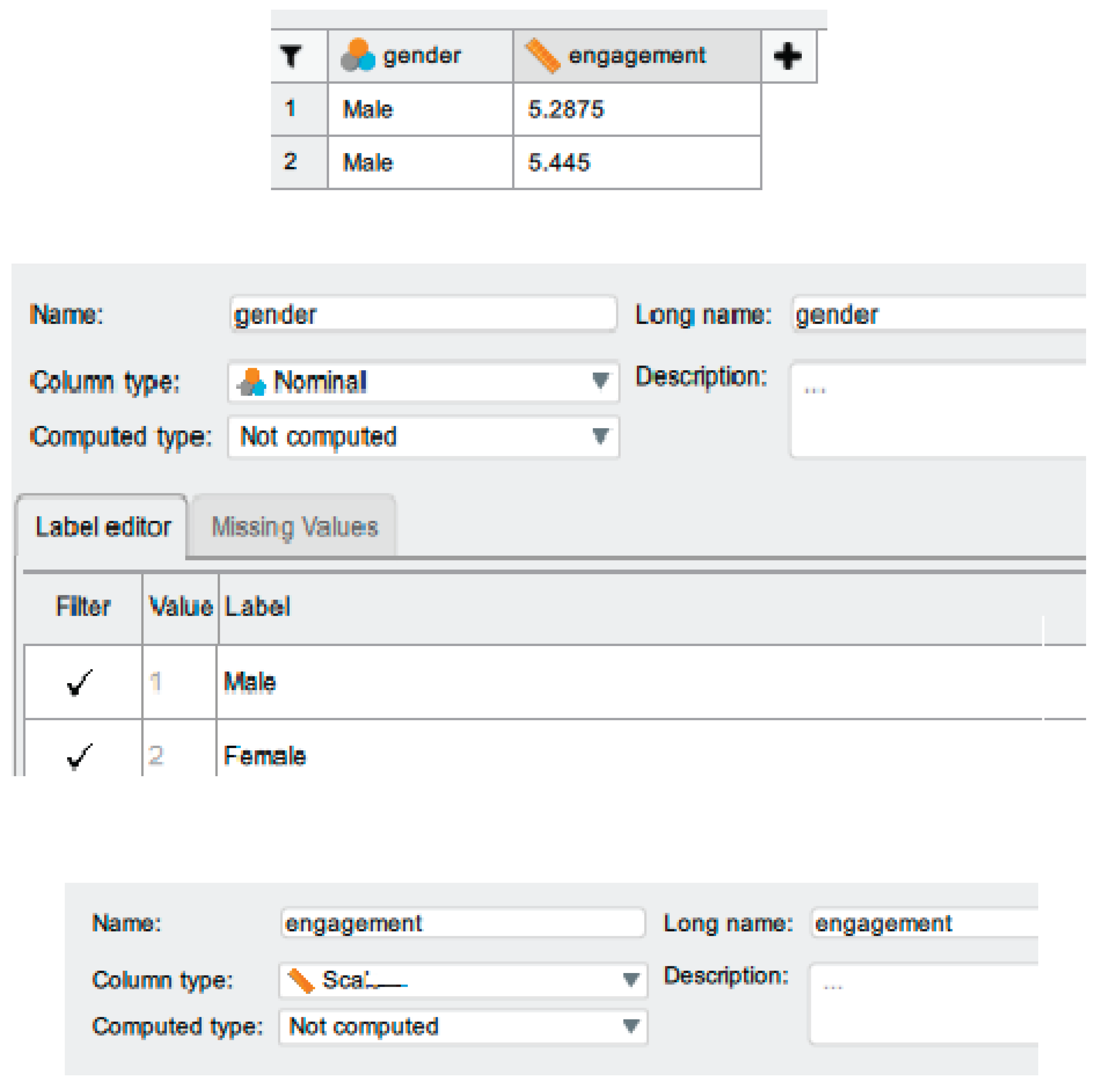
Figure 2.
Independent Samples T-Test Setup with Test Selection, Assumptions, and Additional Statistics Options in JASP.
Figure 2.
Independent Samples T-Test Setup with Test Selection, Assumptions, and Additional Statistics Options in JASP.
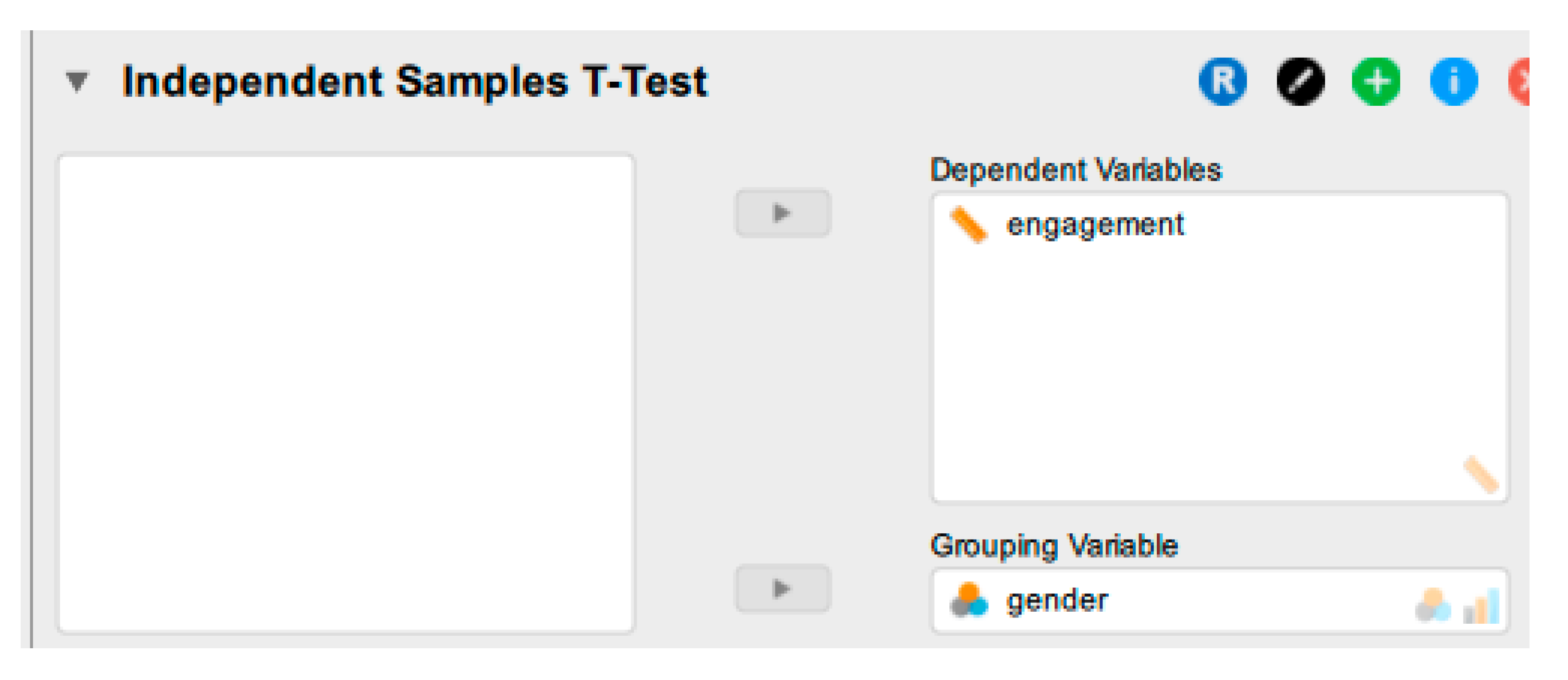
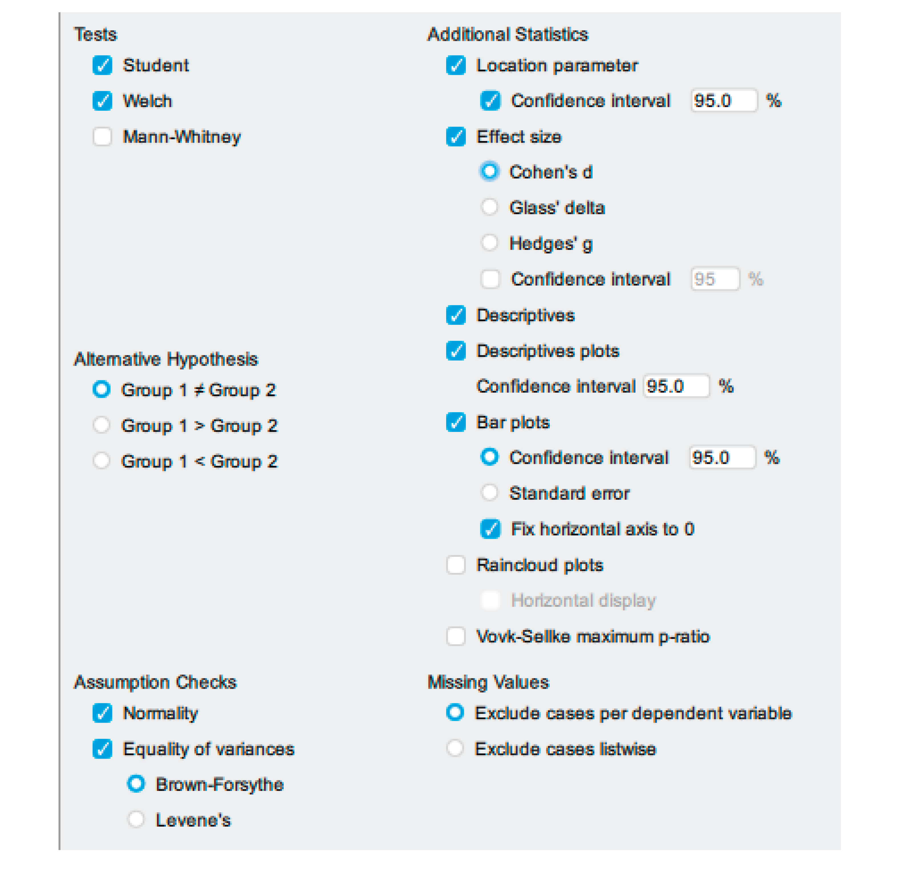
Figure 3.
Results of Independent Samples T-Test with Assumption Checks and Group Descriptive Statistics in JASP.
Figure 3.
Results of Independent Samples T-Test with Assumption Checks and Group Descriptive Statistics in JASP.

Figure 4.
Selection and Results of Student’s and Welch’s Independent Samples T-Tests in JASP.
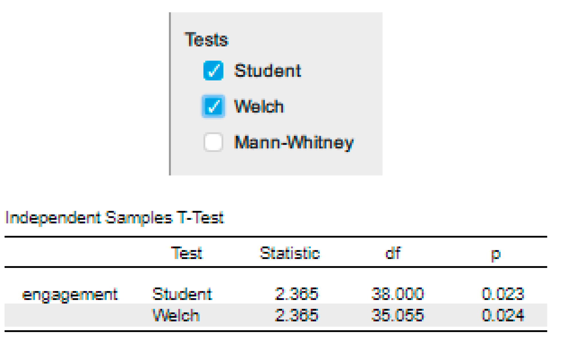
Figure 5.
Additional Statistics and 95% Confidence Interval for Mean Difference in Independent Samples T-Test in JASP.
Figure 5.
Additional Statistics and 95% Confidence Interval for Mean Difference in Independent Samples T-Test in JASP.
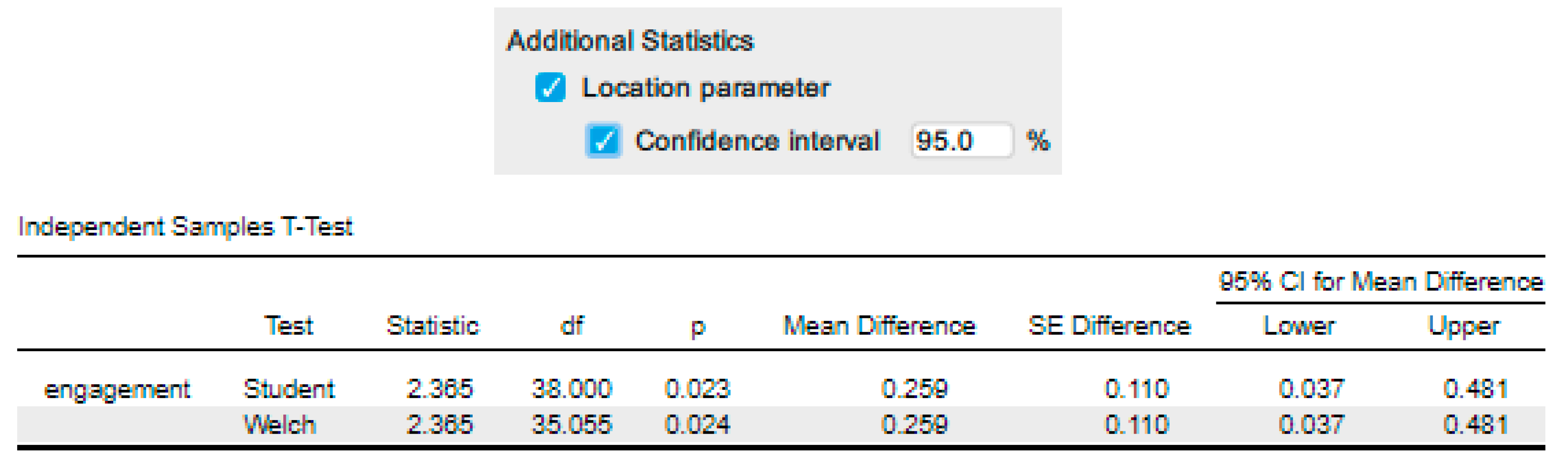
Figure 6.
Independent Samples T-Test Results with Cohen's d Effect Size in JASP.
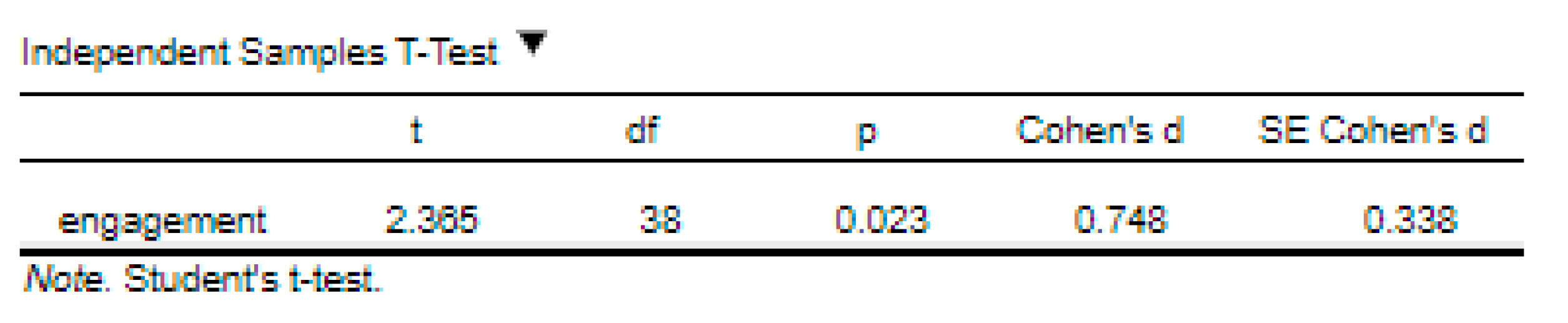
Figure 7.
Mean Engagement Scores by Gender with 95% Confidence Intervals.
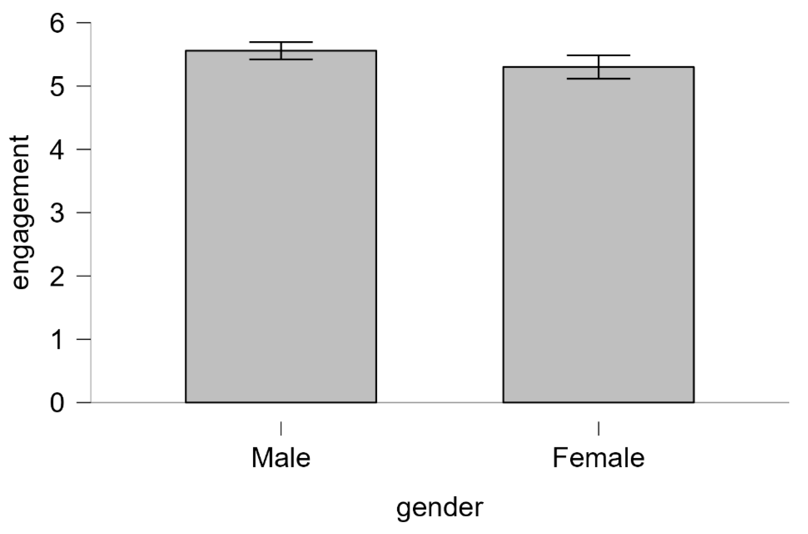

Table 1.
Overview of the Independent-Samples t-Test: Purpose, Terminology, and Applications.
| Field | Details |
|---|---|
| Purpose | The independent-samples t-test tests whether the means of two independent groups differ on a continuous DV. More specifically, it will let us determine whether the differences between these two groups are statistically significant. |
| Test Names | This test is also known by many different names, including: 1. Independent t-test 2. Independent-measures t-test 3. Between-subjects t-test 4. Unpaired t-test 5. Student's t-test |
| Examples |
Medical Testing: Suppose a pharmaceutical company is testing a new drug to treat a certain disease. They administer the drug to one group of patients (the experimental group) and give a placebo to another group (the control group). The I_DV here is the administration of the drug (or placebo), and the DV could be improvement in symptoms or any change in health indicators, measured numerically. Education Research: In an educational study, researchers might investigate the effectiveness of a new teaching method. They could have one group of students taught using the traditional method (control group) and another group taught using the new method (experimental group). The I_DV is the teaching method, and the DV might be the students' test scores or comprehension levels. Healthcare Research: Consider a study examining the quality of life among individuals with a particular chronic disease, such as diabetes. Researchers recruit participants with diabetes and divide them into two groups based on gender: one group consists of males, and the other consists of females. The I_DV in this study is the participants' gender (male or female), while the DV is the quality-of-life score. |
Table 2.
Study designs of the independent-samples t-test.
| No, | Study Designs | Aim | Process | Scenario |
|---|---|---|---|---|
|
Study Design #1 |
Determining if there are differences between two independent groups | This test would be used to determine whether the DV scores differ between the two independent groups. | In this research design, participants are categorised into groups according to a shared characteristic within each group, but not across different groups. |
We have a study design in which we are measuring a DV (e.g., weight, anxiety level, etc.) in two independent groups (e.g., males/females, under 30 years old/30 years old or older, etc.). We wish to know if there is a mean difference in the DV between the two groups. |
| Study Design #2 | Determining if there are differences between interventions | The primary objective is to identify any differences between the two groups, and consequently, between the interventions. |
The study employs a design in which participants are randomly allocated to one of two groups. Each group receives a distinct intervention (for example, Group A receives no intervention, serving as a 'control', while Group B participates in an exercise programme). Typically, the DV of interest (e.g., weight, anxiety level) is measured in each group after the intervention concludes, often using a questionnaire; it may also be assessed during the intervention. Since the DV is not measured prior to the intervention (i.e., without a pre-test score), this type of study design is commonly referred to as a 'post-test only' design. The nature and duration of the interventions may significantly vary. The DV should generally be measured consistently and concurrently across both interventions. Such measurements are frequently conducted at the conclusion of each intervention. |
Participants were randomly assigned to either a six-week exercise training programme or a six-week control group (where no exercise was performed). At the end of each six weeks, participants' blood cholesterol levels were measured as an indicator of health. An independent-samples t-test was then conducted to determine whether significant differences existed in blood cholesterol concentration following the two distinct interventions. The underlying assumption is that any observed differences in the dependent variable, namely blood cholesterol concentration, after the interventions are attributable to the exercise programme. |
| Study Design #3: | Determining if there are differences in change scores | To determine whether the amount of change in the DV differs between two groups that receive different interventions. |
The DV is measured in both groups before and after the intervention. A change score is calculated for each participant by subtracting the pre-test value from the post-test value. An independent-samples t-test is then used to compare these change scores between the two groups to determine whether the intervention produced different levels of change. | A design in which two groups undergo distinct interventions; for example, Group A acts as a control with no intervention, whereas Group B participates in an exercise program. Within each group, the same DV (e.g., weight, anxiety level) is measured at both the pre-intervention and post-intervention phases. Subsequently, a change (gain) score is computed by subtracting the pre-intervention values from the post-intervention values. |
Table 3.
Steps and methods for assumption testing and analysis in JASP.
| Step | Method | Procedure A | Procedure B | Dealing with violations |
|---|---|---|---|---|
| 1 | Study Design | Assumption 1 | Continuous DV | X |
| Assumption 2 | The I_DV has 2 independent categories/groups | X | ||
| Assumption 3 | Independence of observations | X | ||
| 2 | JASP, Data Preparation | Set up the two variables (I_DV and DV) | I_DV: Nominal DV: scale |
- |
| 3 | JASP, Decision | Assumption 4 | Outliers | Reasons: 1. Data entry errors 2. Measurement errors 3. Genuinely unusual values Actions: A. Keeping the outlier(s) 1. Run the non-parametric. 2. Modify the outlier by replacing the outlier's value with one that is less extreme (e.g., the next largest value instead to maintain its rank). 3. Transform the DV. 4. Include the outlier in the analysis anyway. B. Removing the outlier(s) |
| Assumption 5 | Normality | If the data is not normally distributed, we have 4 options: 1. Transform the data. 2. Use a non-parametric test. 3. Carry on regardless. 4. Run test comparisons. |
||
| Assumption 6 | Assumption of homogeneity of variances | Use an adjusted t-statistic based on the Welch method in case of violation. | ||
| 4 | JASP, Analysis and Interpretation | If all the assumptions are met, run the independent sample t-test | 1. From additional statistics, select the location parameter and 95% CI 2. Select Effect Size; cohen’s d. 3. Select Descriptives 4. Select Descriptives Plot. 5. Select Bar Plots |
- |
| 5 | Reporting | 1. Report assumptions 2. Report descriptive statistics: mean, SD, SE. 3. Report t-test results: mean difference, 95% CI, t-value, df, p-value, effect size. |
- |
Table 4.
Assumptions of the independent samples t test.
| No. | Assumption | Details |
|---|---|---|
| Assumption #1 | We have one DV that is measured at the continuous level. | |
| Assumption #2 | We have one IDV that comprises two categorical, independent groups (i.e., a dichotomous variable). | Note: The two groups of the I_DV are also referred to as "categories" or "levels", but the term "levels" is typically reserved for groups possessing an inherent order (e.g., fitness level, with two levels: "low" and "high"). Individuals cannot belong to multiple groups simultaneously. |
| Assumption #3 | Group Independence: It is essential that observations are independent, indicating that there is no correlation among observations within each group of the I_DV nor between the groups. Both groups must be mutually independent. Each participant will contribute only a single data point for one group. | An important distinction is established in statistical analysis when comparing values across different individuals or within the same individual. Independent groups, examined through an independent-samples t-test, consist of groups with no relationship among the participants within each group. This situation most commonly arises due to differences among participants across groups. Independence requires unrelated individuals within each group, avoiding familial relationships. Additionally, participants in one group should not influence those in another group, thereby ensuring experimental integrity. |
| Assumption #4 |
There should be no significant outliers in the two groups of the I_DV with respect to the DV. |
In both groups of the independent dependent variable (IDV), any scores that are markedly different—either exceedingly small or large in comparison to the other scores—are identified as outliers. Outliers may exert a substantial adverse impact on the outcomes by significantly influencing the mean and standard deviation of the respective group, thereby potentially affecting the results of the statistical analysis. The consideration of outliers becomes increasingly important when dealing with smaller sample sizes, as their influence is proportionally greater. Given that outliers can alter the results, it is necessary to determine whether to include them in the data set when conducting an independent samples t-test using JASP. |
| Assumption #5 |
Normality of the DV: The DV should be approximately normally distributed within each I_DV group. The DV should also be measured on a continuous scale and be approximately normally distributed with no significant outliers. |
The presumption of normality is essential when performing a t-test for independent samples. Nonetheless, the independent-samples t-test is regarded as "robust" to breaches of the normality assumption. This implies that certain violations can be tolerated without compromising the validity of the results. Consequently, it is often stated that this test requires approximately normal data. Moreover, as sample sizes increase, the data distribution may deviate significantly from normality; nevertheless, owing to the Central Limit Theorem, the independent-samples t-test can still yield valid conclusions. Additionally, if the distributions are uniformly skewed (e.g., all moderately negatively skewed), this situation is less problematic compared to scenarios where the groups have differently-shaped distributions (e.g., Group A is moderately positively skewed, while Group B is moderately negatively skewed). |
| Assumption #6 |
Homogeneity of variances (i.e., the variance is equal in each group of the I_DV) | This can be tested using Levene's Test of Equality of Variances. If Levene's Test is statistically significant, indicating unequal group variances, we can correct this violation using an adjusted t-statistic based on the Welch method. |
Table 4.
Reporting of assumptions, statistical tests, and interpretation of independent samples t test.
Table 4.
Reporting of assumptions, statistical tests, and interpretation of independent samples t test.
| Category | Reports |
|---|---|
| Assumptions | |
|
Determining if the data has outliers |
‘There were no outliers in the data, as assessed by inspection of a boxplot for values greater than 1.5 box lengths from the edge of the box.’ |
| ‘The data had no outliers, as assessed by inspection of a boxplot’. | |
|
Determining if the data is normally distributed Shapiro-Wilk test for normality |
‘The DV for each level of I_DV was normally distributed, as assessed by Shapiro-Wilk's test (p > 0.05).’ |
| ‘The DV was normally distributed, as assessed by Shapiro-Wilk's test (p > 0.05).’ | |
| Assumption of homogeneity of variances | |
| Assumption of homogeneity of variances was met | ‘Variances were homogeneous for the DV for both groups of the I_DV, as assessed by Levene's test for equality of variances (p = X).’ |
| ‘Variances were homogeneous, as assessed by Levene's test for equality of variances (p = 0.X).’ | |
| Assumption of homogeneity of variances was violated | ‘The assumption of homogeneity of variances was violated, as assessed by Levene's test for equality of variances (p = X).’ |
| Interpreting Results | |
| Descriptive statistics | ‘Data are mean ± standard deviation unless otherwise stated. There were 20 male and 20 female participants. The advertisement was more engaging to males (5.56 ± 0.29) than female viewers (5.30 ± 0.39).’ |
| ‘Data are mean ± standard deviation, unless otherwise stated. There were 20 male and 20 female participants. The mean male engagement score (5.56 ± 0.29) was higher than the mean female engagement score (5.30 ± 0.39).’ | |
|
Mean difference between groups Reporting statistical significance Putting it all together |
‘The male mean engagement score was 0.26 (95% CI, 0.04 to 0.48), higher than the female mean engagement score.’ |
| ‘The male mean engagement score was 0.26 ± 0.11 [mean ± standard error] higher than the female mean engagement score.’ | |
| ‘There was a statistically significant difference between means (p < 0.05); therefore, we can reject the null hypothesis and accept the alternative hypothesis.’ | |
| We can report the results, without the tests of assumptions, as follows: |
‘An independent-samples t-test was run to determine if there were differences in engagement to an advertisement between males and females. The advertisement was more engaging to male viewers (5.56 ± 0.29) than female viewers (5.30 ± 0.39), with a statistically significant difference of 0.26 (95% CI, 0.04 to 0.48), t(38) = 2.365, p = .023.’ |
| Adding in the information about the statistical test we ran, including the assumptions, we have: | ‘Data are mean ± standard deviation unless otherwise stated. There were 20 male and 20 female participants. An independent-samples t-test was run to determine if there were differences in engagement to an advertisement between males and females. The data had no outliers, as assessed by inspection of a boxplot. Engagement scores for each level of gender were normally distributed, as assessed by Shapiro-Wilk's test (p > .05), and variances were homogeneous, as assessed by Levene's test for equality of variances (p = 0.174). The advertisement was more engaging to male viewers (5.56 ± 0.29) than female viewers (5.30 ± 0.39), a statistically significant difference of 0.26 (95% CI, 0.04 to 0.48), t(38) = 2.365, p = 0.023.’ |
|
Calculating and reporting an effect size |
‘Data are mean ± standard deviation unless otherwise stated. There were 20 male and 20 female participants. An independent-samples t-test was run to determine if there were differences in engagement to an advertisement between males and females. The data had no outliers, as assessed by inspection of a boxplot. Engagement scores for each level of gender were normally distributed, as assessed by Shapiro-Wilk's test (p > .05), and variances were homogeneous, as assessed by Levene's test for equality of variances (p = 0.174). The advertisement was more engaging to male viewers (5.56 ± 0.29) than female viewers (5.30 ± 0.39), a statistically significant difference of 0.26 (95% CI, 0.04 to 0.48), t(38) = 2.365, p = 0.023, d = 0.75.’ |
|
Putting it all together |
‘Data are mean ± standard deviation, unless otherwise stated. There were 20 male and 20 female participants. An independent-sample t-test was run to determine if there were differences in engagement to an advertisement between males and females. The data had no outliers, as assessed by inspection of a boxplot. Engagement scores for each level of gender were normally distributed, as assessed by Shapiro-Wilk's test (p > .05), and variances were homogeneous, as assessed by Levene's test for equality of variances (p = 0.174). The advertisement was more engaging to male viewers (5.56 ± 0.29) than female viewers (5.30 ± 0.39), a statistically significant difference of 0.26 (95% CI, 0.04 to 0.48), t(38) = 2.365, p = 0.023, d = .75.’ |
Table 5.
Cohen's d interpretations.
| Effect Size | Strength |
|---|---|
| 0.2 | small |
| 0.5 | medium |
| 0.8 | large |
Disclaimer/Publisher’s Note: The statements, opinions and data contained in all publications are solely those of the individual author(s) and contributor(s) and not of MDPI and/or the editor(s). MDPI and/or the editor(s) disclaim responsibility for any injury to people or property resulting from any ideas, methods, instructions or products referred to in the content. |
© 2025 by the authors. Licensee MDPI, Basel, Switzerland. This article is an open access article distributed under the terms and conditions of the Creative Commons Attribution (CC BY) license (http://creativecommons.org/licenses/by/4.0/).
Copyright: This open access article is published under a Creative Commons CC BY 4.0 license, which permit the free download, distribution, and reuse, provided that the author and preprint are cited in any reuse.


