Submitted:
20 November 2025
Posted:
21 November 2025
You are already at the latest version
Abstract
The scarcity of fault samples significantly impedes the generalization of data-driven diagnosis models for local thermal imbalances in integrated energy systems. To overcome this limitation, this paper proposes a novel knowledge graph-guided conditional generative adversarial network (KG-GAN) framework. The approach begins by constructing a dynamically updatable fault knowledge graph for district heating systems, which explicitly encapsulates pipeline topology, thermodynamic principles, and fault propagation mechanisms. The derived knowledge embeddings are then fused with physics-based constraints into the adversarial learning process, effectively alleviating the issue of physically implausible sample generation that plagues conventional data-centric models. Experimental validation on a district heating platform, involving four common fault types, demonstrates the superiority of our method. With only 100 samples per fault category, a diagnostic model trained on KG-GAN-generated data achieves a classification accuracy of 91.7%, outperforming a GAN-based baseline by 8.3%. Furthermore, t-SNE visualization reveals a 92.3% feature distribution consistency between generated and real samples, confirming the method’s capability to enhance diagnostic robustness and physical interpretability under small-sample conditions.
Keywords:
integrated energy system
; fault diagnosis
; knowledge graph
; generative adversarial network
; small-sample learning
1. Introduction
The rapid advancement of energy transition has positioned Integrated Energy Systems (IES) as pivotal components in the modern energy sector. These systems, however, face significant challenges due to the complex coupling characteristics of electricity-heat-gas multi-energy flows, which introduce various fault risks. Among these, local thermal imbalance represents a particularly critical issue that substantially impacts both user comfort and system efficiency. Current approaches to fault diagnosis primarily fall into two categories: physics-model-driven methods that rely on precise equipment modeling but suffer from limited generalization for strongly coupled faults, and data-driven methods that leverage machine learning and deep learning to extract complex patterns from data while operating independently of detailed physical models [1]. While deep learning methods have shown remarkable capability in learning hierarchical feature representations from high-dimensional signals, they encounter substantial challenges under few-shot scenarios, including overfitting due to sample scarcity [2], feature distribution drift, and the fundamental disconnect between physical mechanisms and diagnostic outcomes.
In addressing data scarcity, Generative Adversarial Networks (GANs) have emerged as a promising solution for data augmentation by learning the probability distribution of training examples [3]. Applications span diverse domains, from Luo et al.’s integration of self-attention into Conditional Deep Convolutional GANs for planetary gearbox fault diagnosis to Lei et al.’s combination of Variational Autoencoders with GANs for steering mechanism fault diagnosis [4]. Beyond mechanical systems, Zhang et al. developed mixed-GANs for pipeline leak detection with expert constraints [5], while Park et al. employed GANs to generate synthetic attack traffic for cybersecurity applications [6]. However, as noted by Gui et al., conventional GANs primarily focus on fitting statistical distributions while lacking explicit mechanisms to ensure adherence to underlying physical laws [8], often resulting in generated samples that are statistically plausible but physically implausible.
Complementary to data-driven approaches, Knowledge Graphs (KGs) offer structured, interpretable domain knowledge to enhance diagnostic models. Recent applications include Meng et al.’s construction of aircraft fault knowledge graphs [9] and Huo et al.’s development of safety knowledge graphs from subway construction accidents [10]. In industrial diagnostics, Mao et al. proposed knowledge aggregation models integrating graph convolutional networks with knowledge graphs [11], while Su et al. introduced graph neural network-based knowledge reasoning for manufacturing processes [12]. While these methods significantly improve interpretability and leverage domain expertise, their performance remains constrained by knowledge graph quality and completeness, and they inherently lack sample generation capabilities.
The emerging trend of hybrid approaches has begun to bridge this gap, with researchers exploring combinations such as Zhou et al.’s incorporation of causal representation learning into dual-GAN architectures [13] and Tong et al.’s integration of GANs with meta-learning for knowledge graph completion [14]. In few-shot learning, Zhao et al. proposed prototype rectification with self-attention mechanism to learn unbiased class prototypes [15]. Despite these advances, a significant research gap persists: no existing work has systematically embedded structured physical constraints from domain-specific knowledge graphs directly into the GAN training process, specifically targeting few-shot thermal fault diagnosis in IES. This gap manifests in three key limitations: the fragmentation between mechanism and data in current approaches, the lack of specificity in utilizing knowledge graphs as generative constraints, and insufficient adaptation mechanisms to ensure knowledge graph quality under limited data conditions.
To address these challenges, this paper proposes a novel Knowledge-Guided Generative Adversarial Network (KG-GAN) framework that fundamentally transforms the generation process from "free creation" to "targeted generation following physical constraints." Our core contributions include constructing a comprehensive IES thermal fault knowledge graph and embedding physical rules into GAN training to ensure generated samples possess both data distribution authenticity and physical law consistency. We design a dynamic knowledge update mechanism for few-shot conditions, enabling self-correction and evolution based on real-time operational data. Furthermore, we establish a complete framework spanning "knowledge construction–constrained generation–trustworthy diagnosis," providing an interpretable solution for industrial fault diagnosis under data scarcity. The proposed method demonstrates three key innovations: dynamic knowledge graph updating for system adaptation, deep integration of physical constraints within the generator, and a comprehensive framework bridging knowledge representation and sample generation for IES thermal fault diagnosis.
2. Theoretical Foundations
2.1. Organizational Structure of Integrated Energy Systems
Integrated energy systems represent the core model for future sustainable energy utilization. They break down the barriers of independent operation between traditional electricity, gas, heating, and cooling systems. Through technological and managerial approaches, they achieve efficient coordination and complementarity among multiple energy sources in terms of time, space, and form. The organizational structure of the integrated energy system studied in this paper is shown in Figure 1.
From a static structural perspective, the IES constitutes a complex system integrating the physical layer energy network with the information layer support system. The physical layer encompasses five key segments: energy production, conversion, storage, transmission/distribution, and consumption. The energy production segment covers both renewable and conventional energy inputs; the conversion segment facilitates cascading transformations between different energy forms; the storage segment mitigates fluctuations in supply and demand; and the transmission/distribution segment delivers energy to consumption points. The energy consumption segment comprises various terminal loads, whose demand characteristics directly drive system operation. The information layer, functioning as the ’nerve centre’, consists of perception, networking, and platform layers, providing perception, communication, computation, and decision support for the physical layer.
During dynamic operation, IES centres on ’multi-energy coupling’ and ’cooperative optimisation’. The system coordinates equipment across all segments through the information layer based on real-time multi-load demands, renewable energy output, and other data. Operational mechanisms include achieving cascading energy utilisation and form conversion via conversion equipment, regulating supply and demand using storage devices, and optimising energy allocation through network optimisation. A closed-loop control system—encompassing sensing, analysis, decision-making, and execution—is created through continuous information flow, with the goal of achieving economic, efficient, low-carbon, and safe operations.
2.2. Multi-Energy Flow Coupling Mechanism
The hallmark of integrated energy systems is the tight coupling and mutual conversion of heterogeneous energy vectors—electricity, heat and gas—across three nested scales: conversion devices, distribution networks and the system layer. The physical laws that govern these interactions are examined below, with emphasis on the deep coupling of electric, thermal and gas flows.
2.2.1. Energy Conversion Device Level
At the device level, combined heat-and-power (CHP) conversion is described by:
Equation (1) is the electricity-to-heat conversion equation for the heat-pump unit, where COP denotes the coefficient of performance that quantifies the conversion efficiency from electric power to thermal output . Equation (2) governs the heat production of the electric boiler; its electric-to-thermal efficiency determines the rate at which electric energy is transformed into heat over time interval . Equation (3) describes the chemical-to-electric energy conversion in the gas turbine, with being the natural-gas mass flow rate and LHV the lower heating value. Equation (4) models the cross-medium heat transfer in the heat exchanger driven by the log-mean temperature difference, where is the heat-transfer rate, U the overall heat-transfer coefficient, A the heat-transfer area, and the log-mean temperature difference.
2.2.2. Energy Transmission Network Level
The transmission constraints at the energy transmission network layer are manifested as follows:
The network loss calculation considers node voltage phase relationships:
The thermal network temperature field evolution is governed by:
Equation (5) embodies the active power balance that must be maintained at all times in the power grid, denoting Kirchhoff’s current law at the power level. In this equation, and denote the input active power and output active power, respectively; denotes the total active power loss.
Network loss calculations consider node voltage phase relationships as shown in Equation (7), where N is the total number of grid nodes; i and j are node indices; and denote the voltage magnitudes at nodes i and j, respectively; and denote the voltage phase angles at nodes i and j, respectively; is the magnitude of the node admittance matrix element; is the phase angle of the node admittance matrix element. The cosine term, determined by the voltage phase difference between the two ends and the equivalent line admittance angle, is crucial for reflecting the direction and magnitude of active power flow.
The hydraulic characteristics of the thermal network follow the Darcy-Weisbach equation in Equation (6), where is the pressure drop in the pipeline and m is the mass flow rate through the pipeline. The resistance coefficient R and the pipe diameter D satisfy an inverse relationship: .
The evolution of the thermal network temperature field is governed by the convection-conduction mechanism described by the one-dimensional unsteady equation in (8), where T is the fluid temperature, t is time, x is the distance along the pipe, v is the flow velocity, h is the combined heat transfer coefficient, is the density, is the specific heat at constant pressure, and is the ambient temperature. The left-hand side of the equation denotes the local temperature change rate, characterizing convective transport effects, while the right-hand side constitutes the environmental heat dissipation term, fully revealing the mechanism of fluid temperature evolution with respect to space and time.
2.2.3. System-Level Coupling
At the system-level coupling layer, energy flow integration is achieved through the energy hub model described by Equation (9):
The output vector contains electrical load and thermal load ; the elements of the efficiency matrix (electricity→electricity), (gas→electricity), (electricity→heat), and (gas→heat) denote dimensionless conversion efficiencies. The input vector comprises electrical input and gas energy input . This matrix equation quantifies, through linear relationships, the coupling process where multi-energy inputs undergo efficiency conversions to satisfy diverse loads.
The fundamental constraint of global energy conservation is as follows:
In the equation, denotes the total energy input to the system; denotes the total energy output; denotes the change in stored energy, where positive values indicate an increase in stored energy and negative values indicate a decrease. This equation directly embodies the First Law of Thermodynamics, ensuring the overall energy balance of the system under any operating conditions.
The multi-energy flow coupling mechanism described in this section provides a direct basis for understanding the fault mechanism of local thermal imbalance in the next section by precisely characterizing the physical laws governing multi-energy flow interactions. It also lays the foundation for the physical constraints established through knowledge graph construction in Chapter 4.
2.3. Mechanism of Local Thermal Imbalance Failure
Local thermal imbalance is a typical failure in district heating networks, with its physical essence stemming from the coupled effects of hydraulic imbalance and thermal response. Failure types induced by hydraulic imbalance include valve sticking—where fixed valve opening causes sudden local resistance changes that disrupt flow distribution—pump efficiency degradation due to worsened head-flow curves leading to insufficient total system flow, and network blockage caused by sharply increased resistance coefficients from local pipe diameter reductions. The following explains some specific principles of thermal imbalance faults.
2.3.1. Valve Sticking Failure
The principle behind valve sticking failures is that valve sticking causes the opening to become fixed, triggering a sudden change in local resistance. The relevant mathematical expression is as follows:
In Equation (11), denotes the flow variation; abnormal changes in the flow coefficient disrupt the designed flow distribution; denotes the pressure difference across the valve, whose abrupt change causes the flow distribution to deviate from the design value.
2.3.2. Pump Efficiency Degradation
The decline in pump efficiency manifests as a degradation of the head-flow curve, with the corresponding mathematical expression as follows:
The efficiency degradation characteristics of a pump are described by the head H, flow rate m, and curve coefficients a, b, and c. Deviations in these coefficients will lead to a decrease in the system’s total flow rate.
2.3.3. Pipe Network Blockage
Pipe network blockages are caused by localized pipe diameter reduction, with the corresponding mathematical expression as follows:
In the equation, R denotes the resistance coefficient, f denotes the friction coefficient, L indicates the pipe length, and D signifies the pipe diameter. When the pipe diameter D decreases by 20%, the resistance coefficient R surges by 300%, leading to upstream pressure buildup and a sharp reduction in downstream flow.
2.3.4. Thermal Inertia Effects
Thermal inertia effects cause the temperature response to lag behind the moment of failure occurrence, meaning there is a time delay between when the failure occurs and when it is effectively detected, as follows:
In the thermal inertia equation (Equation 14), is the time constant, T is the fluid temperature, t is time, and is the setpoint temperature. This results in a fault detection delay of 15–30 minutes.
The time constant causes the fault detection delay. The propagation speed of thermal disturbances is constrained by the fluid flow velocity:
In the thermal disturbance propagation (Equation 15), represents the temperature at position x and time t, denotes the inlet temperature function, and v is the flow velocity. For a pipeline network with a flow velocity of m/s, transmitting a fault signal over a 100m distance takes 100s.
2.3.5. User Load Fluctuations
User load fluctuations create diagnostic interference:
In load fluctuation (Equation 16), denotes the total thermal load, denotes the base load, and denotes the random fluctuation component, whose amplitude can reach up to 20% of the base load.
This section provides a thorough analysis of the physical causes, types, and dynamic characteristics of local thermal imbalance faults in district heating networks. This analysis supports Chapter 2 in precisely modeling faults involving multi-energy flow interactions under local thermal imbalance scenarios.
3. Knowledge Graph Construction and Pattern Representation
Traditional fault diagnosis systems typically treat physical topology modeling and fault knowledge bases as independent modules. To address the disconnect between physical systems and fault knowledge, the proposed knowledge graph models both physical topology and fault modes. By integrating system topology, device characteristics, and fault mechanisms, it provides physical constraints and prior knowledge for the knowledge-guided conditional generation adversarial network introduced in Chapter 4. The physical topology layer performs data injection into the fault knowledge layer, classifying fault samples according to the rules defined within the fault knowledge layer.
3.1. Topological Modeling of District Heating Systems
District heating systems constitute complex networked systems comprising heat sources, heat distribution networks, heat consumers, and associated equipment. To construct a fault knowledge graph, precise modeling of the system topology is essential. Graph theory methods can abstract the physical entities of district heating systems into weighted directed graphs, where nodes represent core system components and edges denote topological connections between components. Edge weights are assigned to characterize key physical parameters. Figure 2 illustrates the complete and specific topology of a basic district heating system.
As shown in Figure 2, the thermal network topology is defined as a weighted multi-graph . The node set V contains key equipment such as heat sources, heat exchange stations, end users, distribution manifolds, and collection manifolds. Each node possesses an attribute vector to record its physical characteristics. The edge set E denotes interconnections between devices, including components such as main pipes, branch pipes, valves, and other components, denoted as . Each edge possesses a direction attribute to describe the flow direction of the medium. The weight set W carries physical parameter information: pipe edge weights correspond to pipe length, pipe diameter, friction coefficient, and design flow rate; valve edge weights include flow coefficient and pressure drop range.
3.2. Fault Mode Mechanism Modeling
Based on the fault mechanism analysis in Section 2, mathematical models for four typical faults—valve sticking, pump failure, pipeline leakage, and sensor drift—were established to address common localized thermal imbalances in district heating systems. Each fault model incorporates explicit physical mechanisms, mathematical expressions, and typical operational manifestations.
Symbol definitions: denotes a uniform distribution over the interval , denotes valve opening, m represents mass flow rate, T indicates temperature, and denotes leakage ratio. Subscript conventions: base denotes normal operating reference values; branch denotes the faulty branch; main denotes the main pipeline; return denotes the return side; reading denotes sensor readings; true denotes actual temperature values.
3.2.1. Valve Sticking Fault Model
The valve sticking fault model derived from the failure mechanism—where mechanical sticking locks the control valve opening at a fixed position, obstructing normal flow regulation—is as follows:
3.2.2. Pump Failure Model
The pump failure model derived from the failure mechanism where system driving force becomes insufficient due to reduced efficiency or complete stoppage of the circulation pump is as follows:
3.2.3. Pipeline Leakage Model
The pipeline leakage model derived from the failure mechanism where thermal medium leakage due to pipeline rupture causes mass loss and pressure drop is as follows:
3.2.4. Sensor Drift Model
The sensor drift model derived from the failure mechanism where zero drift or span drift in temperature sensors causes systematic deviation of measured values from actual values is as follows:
The aforementioned four fault models are formalized as fault mode entities within the knowledge graph. Through attribute mapping, they are associated with their corresponding mathematical expressions and physical rules. These formalized models constitute the core content of the knowledge graph and will be directly encoded as conditional vectors for the KG-GAN in Chapter 4. This enables precise guidance for the generator to synthesize specific types of fault samples, achieving deep integration between physical mechanisms and data generation at the data level.
4. Knowledge Graph Dynamic Update Mechanism
The initially constructed knowledge graph (KG) has static properties, while real physical systems are always in dynamic evolution. To ensure the reliability of the KG in long-term applications, this chapter aims to design a dynamic update mechanism that supports continuous iterative optimization of the KG based on online data. This mechanism can incrementally correct and evaluate the confidence of the knowledge graph based on real-time monitoring data and validation results of generated samples, thereby improving its reliability in practical applications. Through real-time data-driven rule confidence evaluation and conflict resolution, it ensures that the prior knowledge injected into the Knowledge-Guided Generative Adversarial Network (KG-GAN) is accurate and reliable, providing reliable constraints for the generative network, thereby ensuring high quality and high fidelity for the final generated fault samples used for classification training, effectively avoiding invalid or erroneous data generation caused by incorrect knowledge injection.
4.1. Dynamic Update Logic Architecture
The dynamic update steps of the knowledge graph are shown in Figure 3, with inputs including two parts: first, the real-time monitoring data stream , i.e., continuously collected system sensor operation data over time; second, the validation results of generated samples V, used to verify the reliability of existing rules in the knowledge graph.
The update process is divided into three core steps:
- Rule confidence evaluation: Quantifying the reliability of existing rules such as the basic physical laws explained in Section 1.2 and the fault type models defined in Section 2.2;
- Conflict detection: Identifying contradictions between new data and existing knowledge;
- Incremental learning: Correcting the knowledge base based on conflict results.
The output is the updated knowledge graph .
4.2. Rule Confidence Evaluation Model
The rule confidence evaluation model quantitatively assesses the credibility of existing fault rules (Section 2.2) in real environments, providing a basis for differentiated knowledge updates, prioritizing the correction of unreliable knowledge.
Define rule confidence as shown in Equation (21):
Where, is the number of samples conforming to the rule; is the total number of samples triggering the rule; t is the current time, is the last update time, and the time decay factor is calculated as:
Update strategies are dynamically adjusted according to confidence values:
The above model quantifies the reliability of rules, enabling intelligent update strategies. High-confidence rules are considered reliable knowledge and can stably guide data generation; low-confidence rules are flagged and prioritized for update, preventing them from generating erroneous fault data that contaminates the training set, thereby protecting the training effect of small-sample classification models.
4.3. Conflict Resolution and Incremental Learning
The conflict detection mechanism based on conservation laws and the hierarchical incremental update strategy ensure the physical rationality and topological consistency of the KG when absorbing new knowledge. The updated KG will be fed back to the knowledge encoding and constraint modules of KG-GAN in Chapter 4.
Conflict resolution occurs when new data conflicts with old knowledge, performing verification and correction based on physical laws to ensure the correctness of the KG. Constraint verification is performed based on physical conservation laws (Equation 24). When monitoring data violate energy conservation, mass conservation, or hydraulic balance constraints, the system automatically triggers conflict detection:
Where, P represents thermal power (kW), is the allowable error threshold for equipment. m is mass flow (kg/s), is the system pressure drop (kPa), is the allowable overpressure coefficient.
Heating systems face dynamic changes such as topological modifications, equipment aging, and discovery of new fault modes during operation cycles. If the static graph is not iterated, the prior knowledge it carries will gradually deviate from reality, leading to decreased accuracy in subsequent fault sample generation and fault diagnosis. Therefore, incremental learning, through continuous integration of online data to achieve dynamic updates of the graph, is key to ensuring its long-term reliability and application value.
Considering that the heating system topology has a clear "node-edge" structural characteristic, its dynamic changes can be clearly divided into two categories: entity addition and parameter drift. Generic update methods struggle to balance iteration efficiency and physical compliance. Based on this, the following designs a hierarchical update strategy for node-level updates and edge relationship corrections, tailored to this topological characteristic of heating systems, to achieve refined, physically credible incremental optimization of the graph.
4.3.1. Node-level Update
During the operation cycle of the heating system, pipeline network expansion, equipment additions, or discovery of new fault modes may require adding corresponding nodes to the graph. Considering the strong coupling between core attributes of different devices and system physics, node expansion needs to be differentiated by device type:
The above equation defines the attributes of heat source nodes, pipe nodes, and valve nodes, applied to heating systems containing these three types. In the key parameters of heat source node characteristics, ID represents the type or identifier of the heat source; represents the design heating power of the heat source; represents the design outlet temperature of the heat source. In the key parameters of pipe node characteristics, ID represents the type or identifier of the pipe; L is the length of the pipe; D is the diameter of the pipe; f is the friction factor of the pipe; represents the maximum design mass flow of the pipe. In the key parameters of valve node characteristics, ID represents the type or identifier of the valve; represents the flow coefficient of the valve; represents the adjustable pressure drop range of the valve. Among these, attribute inheritance from adjacent nodes means that newly added pipes automatically inherit the D (pipe diameter) and (design flow) of connecting equipment, and newly added valves inherit the (operating pressure drop) from upstream and downstream.
4.3.2. Edge Relationship Correction
Edge relationship correction adopts a weighted fusion strategy under hydraulic constraints: on one hand, achieving smooth transition of old and new parameters through a weighting formula. Long-term monitoring data with high confidence can reduce the weight coefficient value, allowing new parameters to dominate the correction faster; short-term data with low confidence increase the value, retaining the stability of old parameters and avoiding abrupt changes in graph parameters.
The update of pipeline connection relationships uses the weighted fusion formula under hydraulic constraints as follows:
Where, represents the final corrected hydraulic parameter; represents the original stable parameter value in the system before correction, with historical credibility; is the parameter change value calculated based on new monitoring data; represents the hydraulic constraint factor; is the weight coefficient.
Simultaneously, the correction process must strictly satisfy the hydraulic constraint function based on fluid mechanics. Define the constraint function satisfying:
Where, , f is the friction factor, v is the flow velocity (m/s).
This constraint strongly binds parameters such as friction factor and flow velocity to the actual pressure drop, ensuring that the corrected edge relationship parameters not only fit the monitoring data but also avoid physical contradictions such as "excessive flow velocity leading to pressure drop exceeding pipeline pressure limit" and "abnormally small friction factor violating resistance characteristics", fundamentally guaranteeing the physical credibility of the graph’s edge relationships, providing reliable resistance characteristics for subsequent fault simulation and data generation.
5. Knowledge-Guided Conditional Generative Adversarial Network
5.1. Background and Motivation
Traditional Generative Adversarial Networks (GANs) face fundamental challenges when generating fault data for integrated energy systems: the generation process lacks prior knowledge guidance, making it impossible to ensure that generated samples comply with complex physical laws and system topology logic. This limitation often results in generated data that, while statistically similar to real data, violates fundamental engineering principles, thereby reducing its practical utility for training reliable diagnostic models.
To address this critical issue, this paper proposes a Knowledge Graph-guided Conditional Generative Adversarial Network (KG-GAN) framework. The core innovation lies in the deep integration of physical knowledge from the dynamic knowledge graph with the data generation capability of GANs. This integration transforms the generation process from "free creation" to "targeted generation following physical constraints," effectively solving the problem of scarce fault data for local thermal imbalance under small-sample conditions.
5.2. KG-GAN Overall Framework
The overall architecture of KG-GAN, as illustrated in Figure 4, consists of three core modules: the knowledge graph condition encoder, the physically-constrained generator, and the dual discriminator. The condition vector , derived from the knowledge graph, is simultaneously fed into both the generator G and discriminator D, ensuring that the entire generation process is guided and constrained by domain knowledge.
The workflow can be conceptually described as follows: The knowledge graph condition encoder extracts structured knowledge from the dynamic knowledge graph and encodes it into a condition vector . This vector carries semantic information about system topology, physical parameters, and fault patterns. The generator G then uses this condition vector, along with random noise , to generate synthetic fault samples. Crucially, the generator incorporates multiple physical constraints to ensure the generated data complies with engineering logic. The discriminator D employs a dual discrimination mechanism, evaluating both the authenticity of the data and its compliance with physical rules.
5.3. Knowledge Graph Condition Encoding
Condition encoding is the process of transforming structured knowledge from the knowledge graph into a condition vector , which serves as semantic guidance for the generation process. This encoding captures multiple aspects of domain knowledge:
Topology Structure Encoding: The original feature vector of the n-th topology node is transformed into a dense vector through an embedding matrix:
This transformation converts discrete engineering attributes into continuous vector representations, enabling subsequent neural networks to process structured knowledge while preserving topological relationships between entities.
Physical Parameter Constraints: Edge weight physical parameters are extracted to construct hydraulic constraint equations:
This design cleverly embeds engineering equations (such as the Darcy formula in Equation 7) into the neural network, ensuring that generated data respects fundamental physical laws.
Fault Pattern Encoding: Long Short-Term Memory (LSTM) networks process temporal fault characteristic sequences:
This temporal processing is particularly important for gradual faults, as LSTM can capture state evolution processes. The output represents the dynamic encoding of fault patterns.
The final condition vector provides multi-dimensional semantic guidance for the generation process, ensuring that generated samples are not only statistically similar to real data but also physically plausible.
5.4. Physically-Constrained Generation Control
To fundamentally guarantee the rationality of generated samples, multiple physical constraints are integrated into the generator:
Topology Structure Constraints: Graph Convolutional Networks (GCNs) inject pipeline connection relationships:
This formulation enables the generator to understand and respect the actual connection relationships in the pipeline network, ensuring that generated data reflects realistic topological constraints.
Energy Conservation Constraints: A physical verification module is added to the output layer:
This constraint ensures that the heat-related portions of the generated data are consistent with the physical heat calculated from the flow rate and temperature data, with an error tolerance of less than 5%.
Fault Propagation Constraints: A conditional mask matrix is designed to restrict unreasonable fault feature combinations:
Based on the fault association rules in the knowledge graph, this mask prevents physically impossible combinations of fault characteristics from appearing in the generated data.
5.5. Dual Discrimination Mechanism
To ensure that KG-GAN generates data that conforms to both real data distribution and logical constraints, the traditional GAN loss function is specifically improved:
The traditional adversarial loss function:
An additional rule consistency loss is introduced to specifically penalize logical conflicts between generated data and knowledge graph rules:
The total loss function combines both objectives:
This dual discrimination mechanism—combining data authenticity discrimination with physical compliance discrimination—forms a dual quality assurance system for generated data. The weight coefficient enables dynamic weighting of key constraints, allowing the model to adaptively strengthen the constraint effectiveness of high-confidence rules.
6. Experimental Setup and Analysis
6.1. Experimental Environment and Data Setup
The experimental platform was developed based on Python 3.9, utilizing deep learning frameworks including NumPy 1.21, Pandas 1.3, Scikit-learn 1.0.2, and TensorFlow 2.15.0. The primary objective of this platform is to accurately reproduce the physical evolution process of local thermal imbalance faults in district heating systems, providing a reliable simulation environment for knowledge graph construction and KG-GAN model training.
The constructed district heating system model includes one heat source node, two user building nodes, and a complete connecting pipeline network system. Key monitoring and control equipment include regulating valves, circulation pumps, temperature sensors installed at supply and return water sides, and flow sensors deployed on main and branch pipelines. The system topology structure is shown in Figure 5, demonstrating the complete correlation among physical components, monitoring equipment, and fault types.
System operating parameters were set with reference to typical design values from northern urban district heating projects. Specific parameter ranges are shown in Table 1. Parameter fluctuation amplitudes were determined according to the permissible system operation deviations specified in the Code for Construction and Acceptance of Urban Heating Pipeline Networks, ensuring engineering rationality of the simulation scenario.
To simulate small-sample fault diagnosis scenarios, a simulation dataset containing one normal operating condition and four typical fault types was generated based on the local thermal imbalance fault mechanism described in Section 2. Each fault type contains 100 samples, covering the complete lifecycle characteristics from fault initiation with minor parameter deviations, through rapid parameter fluctuations during fault development, to stable parameter states during fault stabilization. The data generation process strictly adheres to multi-energy flow coupling equations and fault mechanism equations, ensuring physical consistency.
6.2. Knowledge Graph Construction and Validation
A structured fault knowledge graph for district heating system local thermal imbalance faults was constructed based on a three-layer association logic of physical components, fault modes, and monitoring data, achieving formal expression and computable invocation of engineering knowledge. The node layer design includes two core node types: physical component nodes and fault type nodes. Physical component nodes cover heat sources, main pipelines, branch pipelines, regulating valves, circulation pumps, temperature sensors, and flow sensors, with each node associated with specific physical attributes. Fault type nodes include valve stuck, pump failure, pipeline leakage, and sensor drift, with node attributes related to fault characteristic parameters. The relationship layer defines three semantic relationships: causes describing the causal relationship between faults and parameter anomalies, controls describing the control relationship between equipment and system parameters, and monitored by describing the monitoring relationship between parameters and sensors. The rule layer maps mathematical models of four fault types into rules callable by the graph, ensuring consistency between knowledge representation and physical mechanisms.
Structural rationality and engineering accuracy of the knowledge graph were verified through expert review and physical consistency checking. Node association relationships are consistent with the actual system topology, fault propagation paths align with engineering practical experience, and physical constraint rules match multi-energy flow coupling equations precisely. Figure 6 shows the complete knowledge graph structure, where blue nodes represent physical components, red nodes identify fault types, and edge relationships represent component associations and fault propagation logic, providing reliable prior knowledge support for subsequent KG-GAN models. The state of graph nodes can continuously change with fault severity, providing fine-grained control dimensions for the generator. Different from traditional GAN random sampling, this method generates progressively worsening fault scenarios based on node attribute offsets, enabling expansion of diverse data covering edge conditions even with scarce samples, thereby enhancing classifier feature discrimination capability.
6.3. Experimental Results and Analysis
The KG-GAN model training dynamics demonstrate excellent convergence characteristics, as illustrated in Figure 7 which tracks the evolution of accuracy and loss metrics throughout the training process. Both training and validation accuracy show continuous improvement, stabilizing after 20 epochs with final values reaching 93.2% and 91.7% respectively. The minimal difference between training and validation accuracy, maintained below 2%, indicates strong model generalization capability. The generator and discriminator losses exhibit gradual convergence, stabilizing within the range of 0.25-0.3 after 20 epochs, with the loss difference consistently below 0.05. This balanced convergence pattern demonstrates that the adversarial training has successfully reached Nash equilibrium, ensuring stable model performance.
The quality of generated data was comprehensively evaluated through multiple validation approaches. Feature distribution consistency was examined using t-SNE dimensionality reduction to map high-dimensional fault features to a two-dimensional space. As shown in Figure 8, the feature clusters of generated data exhibit remarkable consistency with simulated real data in both shape and position. The analysis reveals excellent aggregation within the same fault type clusters and significant separation between different fault type clusters, achieving an overall feature distribution consistency of 92.3%. This high consistency confirms that the generated data successfully captures the core distribution patterns of real data.
To further analyze the distribution characteristics, we conducted detailed statistical tests on the feature embeddings. The high-dimensional feature vectors were projected into two-dimensional space using t-SNE with a perplexity of 30 and learning rate of 200. The resulting visualization clearly demonstrates the effectiveness of our approach in maintaining the intrinsic structure of the original data distribution.
Parameter distribution matching was further investigated through density distribution analysis of key parameters. Figure 9 demonstrates consistent distribution curve trends for supply water temperature, return water temperature, main flow rate, branch flow rates, and valve opening between generated and simulated real data. The peak position deviation remains within 5% across all parameters, with no significant distribution shifts observed. This close alignment in statistical distribution verifies the effective matching between generated data and real data in terms of parameter characteristics.
The density distribution analysis employed kernel density estimation with Gaussian kernels to provide smooth probability density functions for each parameter. This method allows for comprehensive comparison of the underlying distributions beyond simple statistical moments, revealing subtle differences that might be overlooked by conventional statistical tests.
The discrimination capability of different fault modes was evaluated by analyzing characteristic parameter patterns across various fault types. Valve stuck samples consistently exhibit significant decreases in branch flow accompanied by fixed valve opening positions, while pump failure samples demonstrate main flow rates dropping below critical thresholds with corresponding decreases in branch flows. Pipeline leakage samples display distinctive patterns of abnormal increases in main flow rate coupled with decreased branch flows, and sensor drift samples show systematic deviations between temperature readings and actual values. These distinct parameter signatures confirm that the generated data effectively differentiates between fault modes and maintains diagnostic feature effectiveness.
Time series evolution compliance was assessed by examining the temporal behavior of generated data parameters. As illustrated in Figure 10, the temperature parameter variations adhere to thermal inertia equations with appropriate fault response delays of approximately 15 minutes, while flow parameter changes follow hydraulic constraint equations with smooth transition processes. The absence of parameter mutations or other physically implausible phenomena validates the temporal evolution compliance of the generated data, ensuring its reliability for time-series based fault diagnosis applications.
7. Conclusion
This paper addresses the small-sample problem in fault diagnosis for local thermal imbalance in integrated energy systems by proposing a knowledge graph-guided generative adversarial network framework. By deeply integrating structured knowledge from dynamic knowledge graphs into the generation process, we ensure that the generated data maintains physical rationality and engineering value. Experimental results demonstrate that our method outperforms traditional approaches across multiple quantitative metrics, providing an effective solution for industrial fault diagnosis under small-sample conditions.
The key experimental findings include: (1) The KG-GAN framework achieved 91.7% classification accuracy with only 100 samples per fault category, as shown in Figure 7; (2) Feature distribution analysis in Figure 8 revealed 92.3% consistency between generated and real samples; (3) Parameter distribution matching in Figure 9 confirmed the physical plausibility of generated data; (4) Time series validation in Figure 10 demonstrated compliance with thermal inertia and hydraulic constraints.
While the current work has achieved promising results, several aspects warrant further investigation. Future research could explore the extension of this framework to more complex coupled faults and its application to larger-scale systems. Additionally, the integration of more sophisticated knowledge representation and reasoning mechanisms could further enhance the framework’s capability to handle increasingly complex industrial scenarios.
References
- Luo, J. , Huang, J. Y., Ma, J. C., & Liu, S. Y. (2024). Application of self-attention conditional deep convolutional generative adversarial networks in the fault diagnosis of planetary gearboxes. Proceedings of the Institution of Mechanical Engineers, Part O: Journal of Risk and Reliability, 238, 260–273. [CrossRef]
- Zeng, W. , & Xiao, Z. Y. (2024). Few-shot learning based on deep learning: A survey. Mathematical Biosciences and Engineering, 21, 679–711. [CrossRef]
- Goodfellow, I. , Pouget-Abadie, J., Mirza, M., Xu, B., Warde-Farley, D., Ozair, S., et al. (2020). Generative adversarial networks. Communications of the ACM. ( 63(11), 139–144.
- Lei, T. F. , Pei, Z. Y., Pan, F., Li, B., Xu, Y. S., Shao, H. D., et al. (2024). A novel data augmentation method for steering mechanism fault diagnosis based on variational autoencoding generative adversarial networks with self-attention. Measurement Science and Technology, 35. [CrossRef]
- Zhang, H. G. , Hu, X. G., Ma, D. Z., Wang, R., & Xie, X. P. (2022). Insufficient data generative model for pipeline network leak detection using generative adversarial networks. IEEE Transactions on Cybernetics. P. ( 52(7), 7107–7120. [CrossRef]
- Park, C. , Lee, J., Kim, Y., Park, J. G., Kim, H., & Hong, D. (2023). An enhanced AI-based network intrusion detection system using generative adversarial networks. IEEE Internet of Things Journal, 2023; 10, 2330–2345. [Google Scholar] [CrossRef]
- Lupión, M. , Cruciani, F., Cleland, I., Nugent, C., & Ortigosa, P. M. (2024). Data augmentation for human activity recognition with generative adversarial networks. IEEE Journal of Biomedical and Health Informatics, M. ( 28(4), 2350–2361. [CrossRef]
- Gui, J. , Sun, Z. A., Wen, Y. G., Tao, D. C., & Ye, J. P. (2023). A review on generative adversarial networks: Algorithms, theory, and applications. IEEE Transactions on Knowledge and Data Engineering, 35(4), 3313–3332. [Google Scholar]
- Meng, X. Z. , Jing, B., Wang, S. L., Pan, J. X., Huang, Y. F., Jiao, X. X., et al. (2024). Fault knowledge graph construction and platform development for aircraft PHM. Sensors, 24. [CrossRef]
- Huo, X. S. , Yin, Y., Jiao, L. D., & Zhang, Y. (2024). A data-driven and knowledge graph-based analysis of the risk hazard coupling mechanism in subway construction accidents. Reliability Engineering and System Safety, 250.
- Mao, Z. H. , Wang, H., Jiang, B., Xu, J., & Guo, H. F. (2024). Graph convolutional neural network for intelligent fault diagnosis of machines via knowledge graph. IEEE Transactions on Industrial Informatics. F. ( 20(5), 7862–7870.
- Su, C. , Jiang, Q., Han, Y., Wang, T., & He, Q. C. (2025). Knowledge graph-driven decision support for manufacturing process: A graph neural network-based knowledge reasoning approach. Advanced Engineering Informatics, 64. [CrossRef]
- Zhou, X. K. , Zheng, X. Z., Shu, T., Liang, W., Wang, K. I.-K., Qi, L. Y., et al. (2025). Information theoretic learning-enhanced dual-generative adversarial networks with causal representation for robust OOD generalization. IEEE Transactions on Neural Networks and Learning Systems, 2025; 36, 2066–2079. [Google Scholar]
- Tong, W. M. , Chu, X., Li, Z. W., Tan, L. G., Zhao, J. X., & Pan, F. (2024). Generative adversarial meta-learning knowledge graph completion for large-scale complex knowledge graphs. Journal of Intelligent Information Systems, 62, 1685–1701.
- Zhao, P. , Wang, L., Zhao, X. Y., Liu, H. T., & Ji, X. (2024). Few-shot learning based on prototype rectification with a self-attention mechanism. Expert Systems with Applications, 249. [CrossRef]
Figure 1.
Organization Structure Diagram of Integrated Energy System.
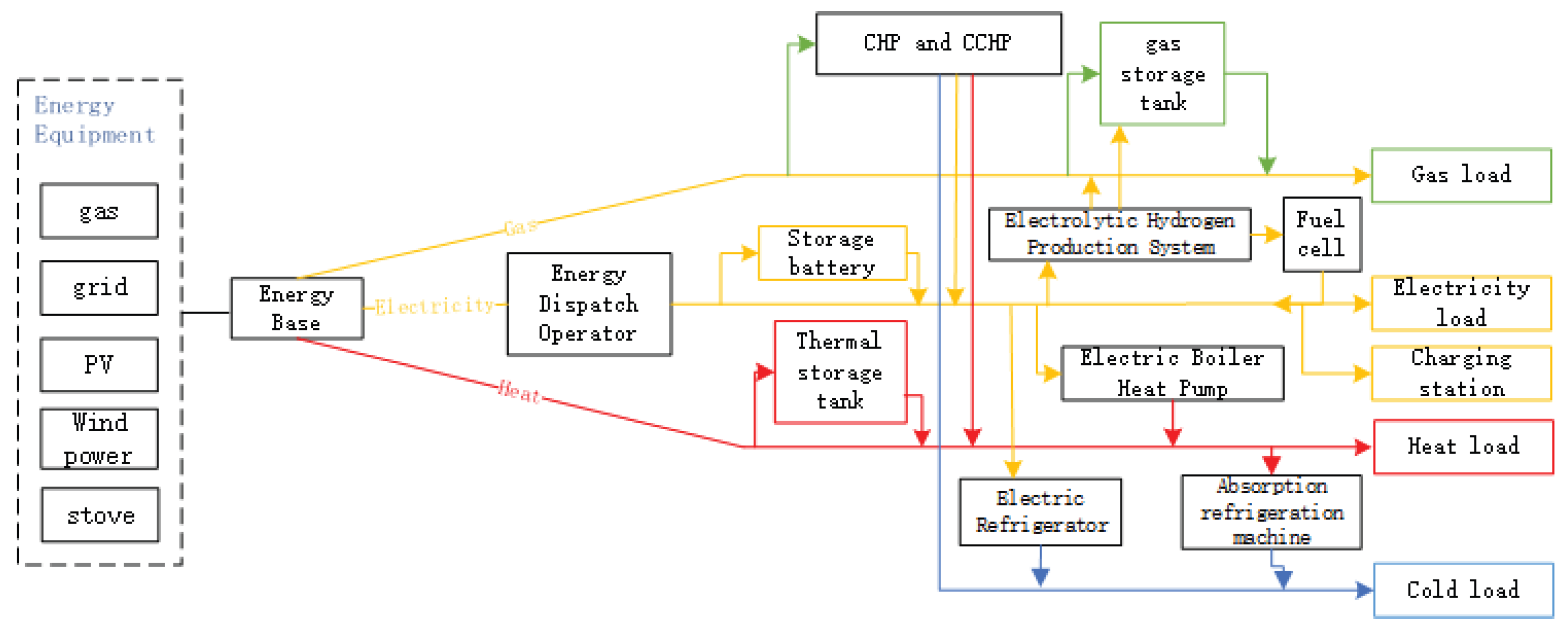
Figure 2.
District Heating System Topology Structure Diagram.
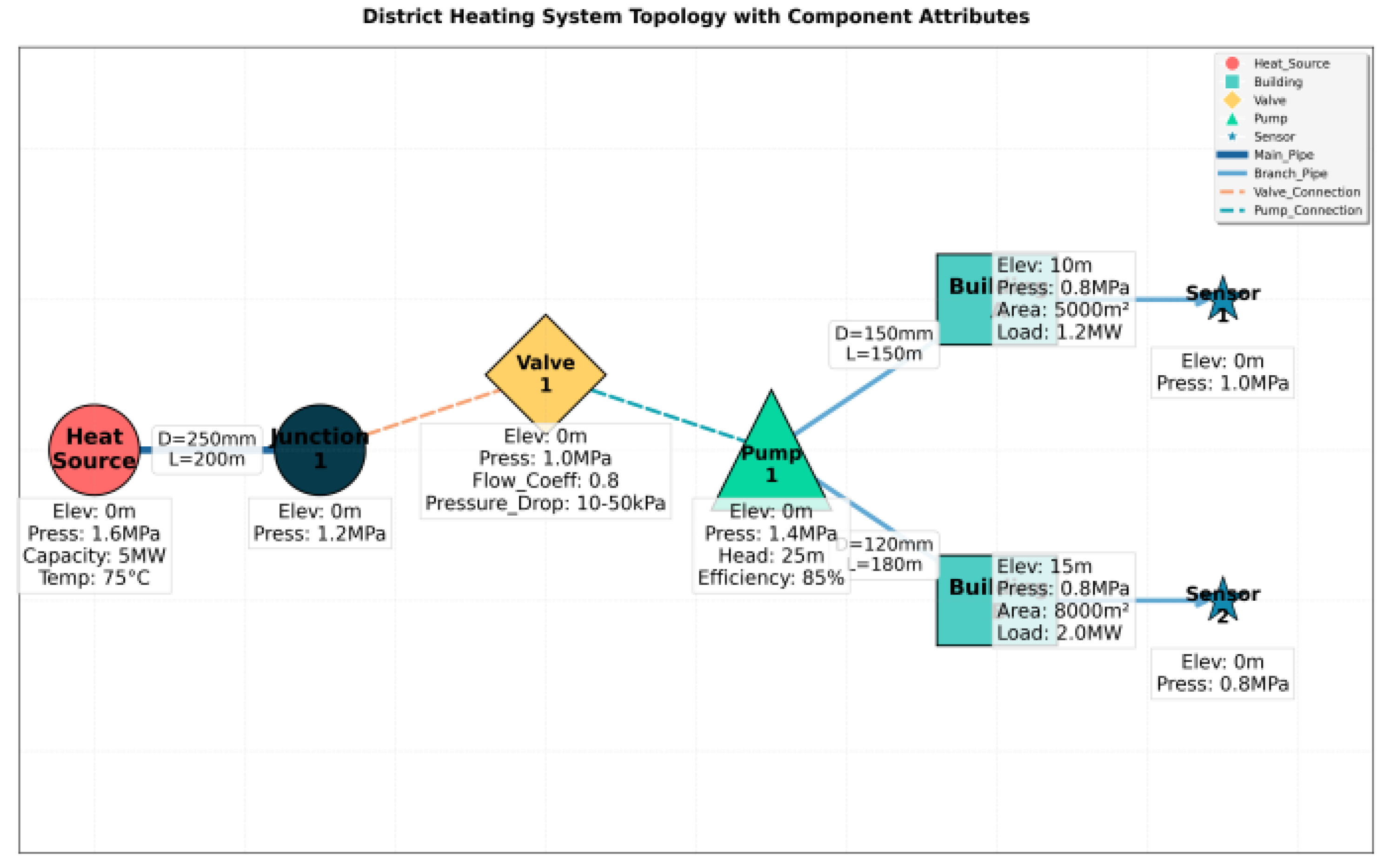
Figure 3.
Schematic Diagram of Knowledge Graph Dynamic Update Steps.
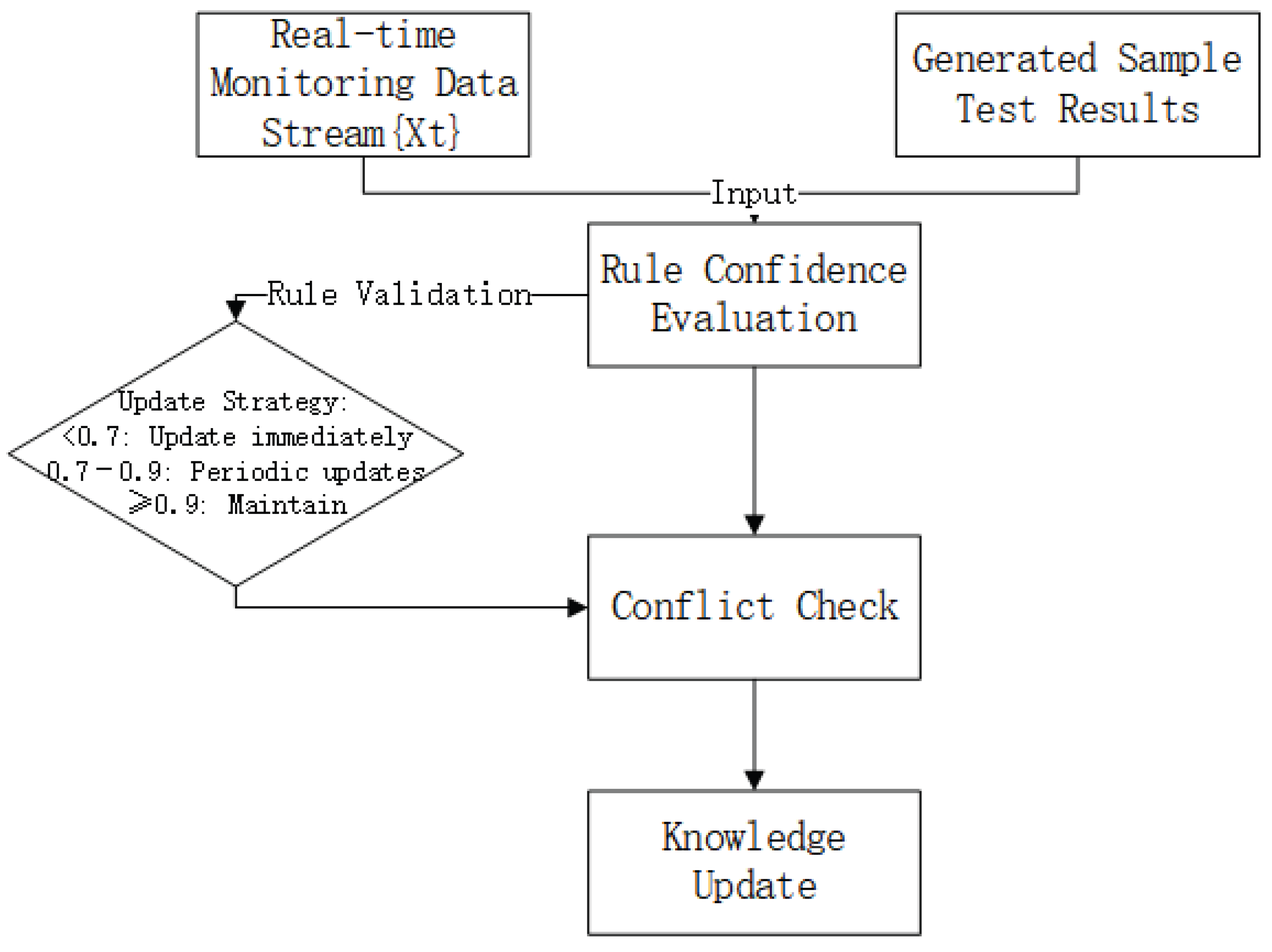
Figure 4.
Overall architecture of Knowledge-Guided Generative Adversarial Networks.
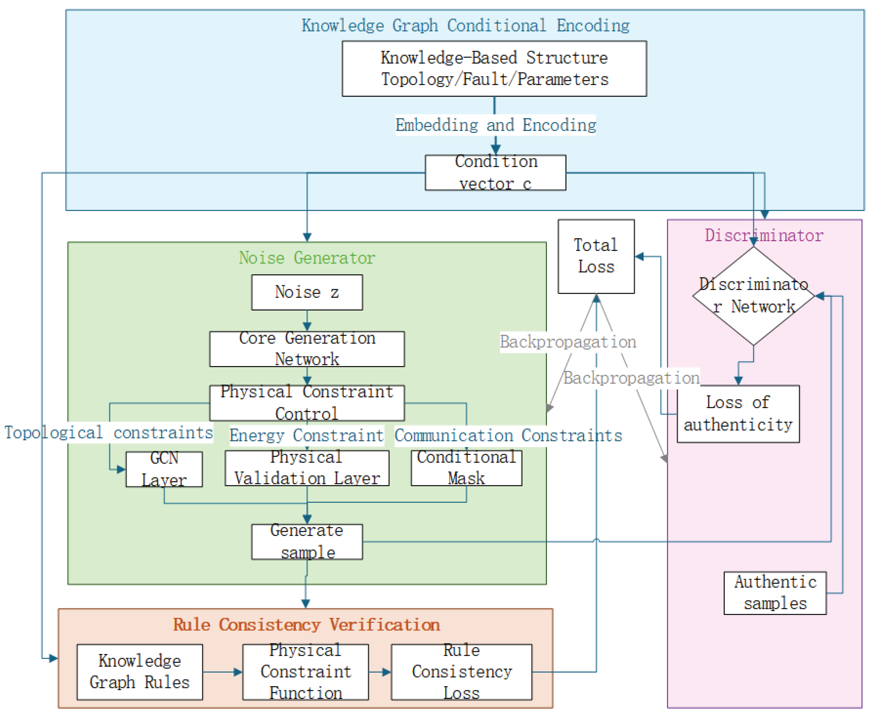
Figure 5.
District heating system topology.
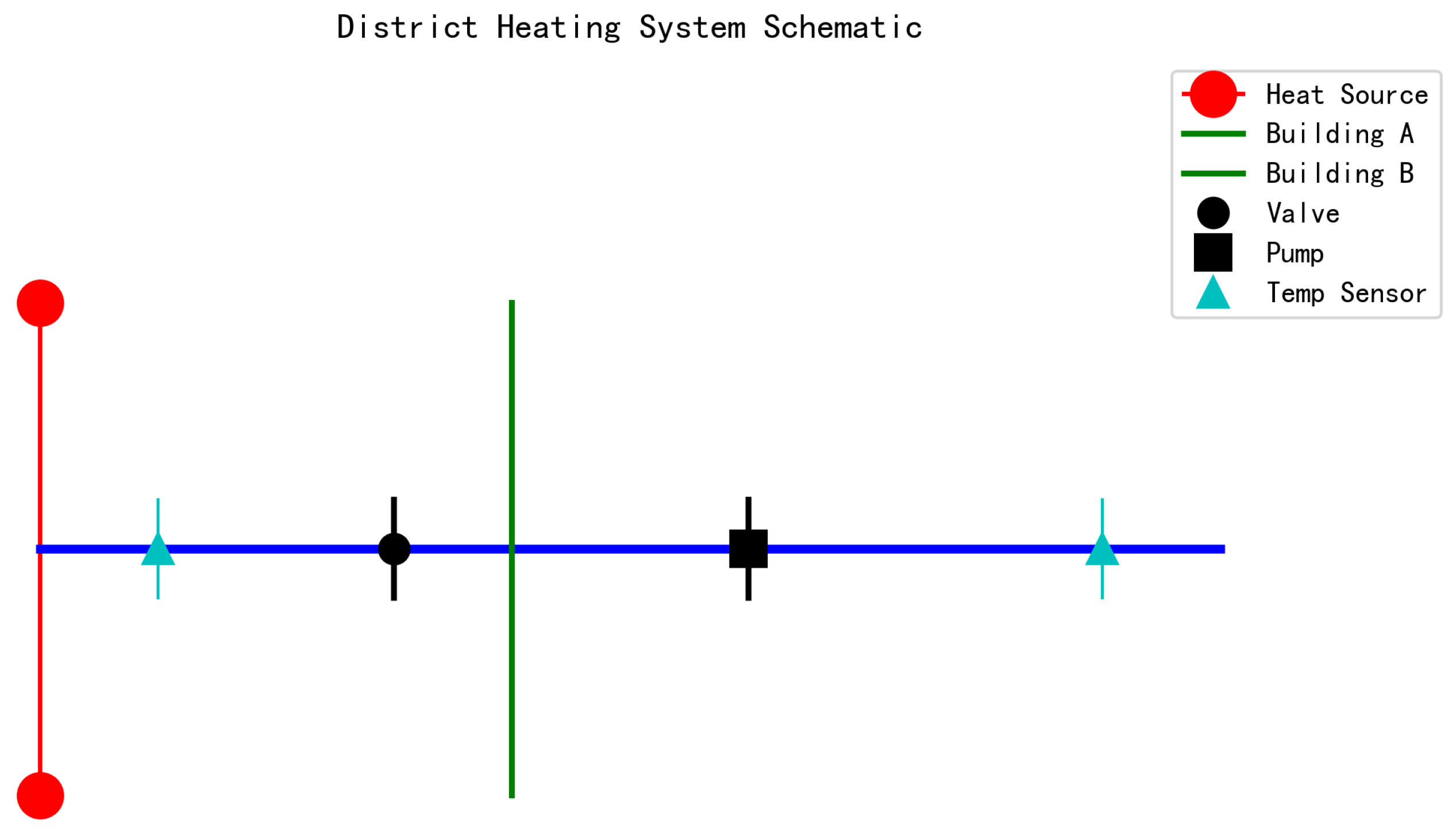
Figure 6.
Fault knowledge graph of thermal systems.
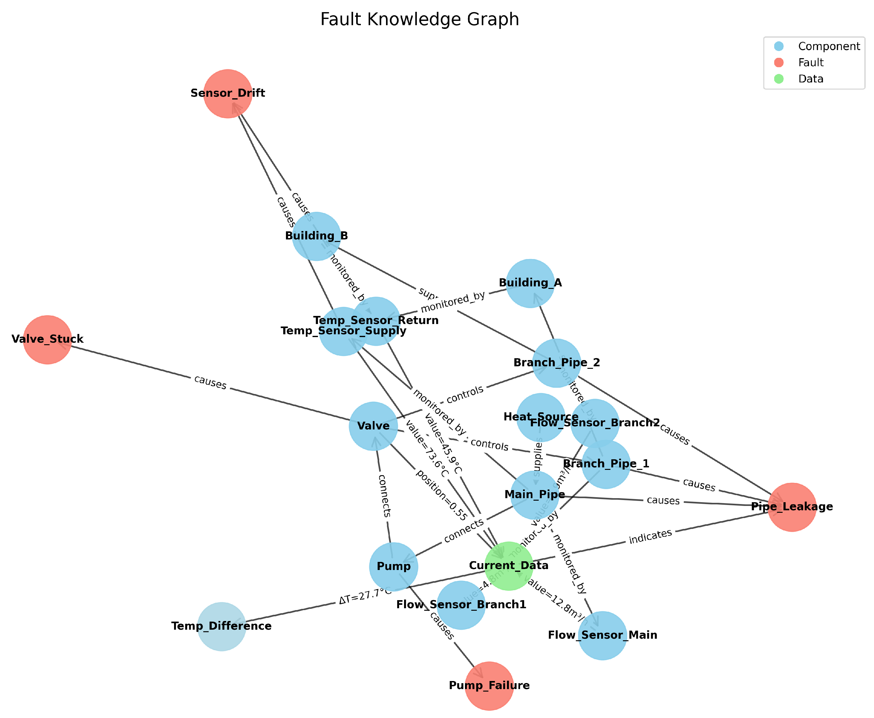
Figure 7.
Evolutionary process of model training.
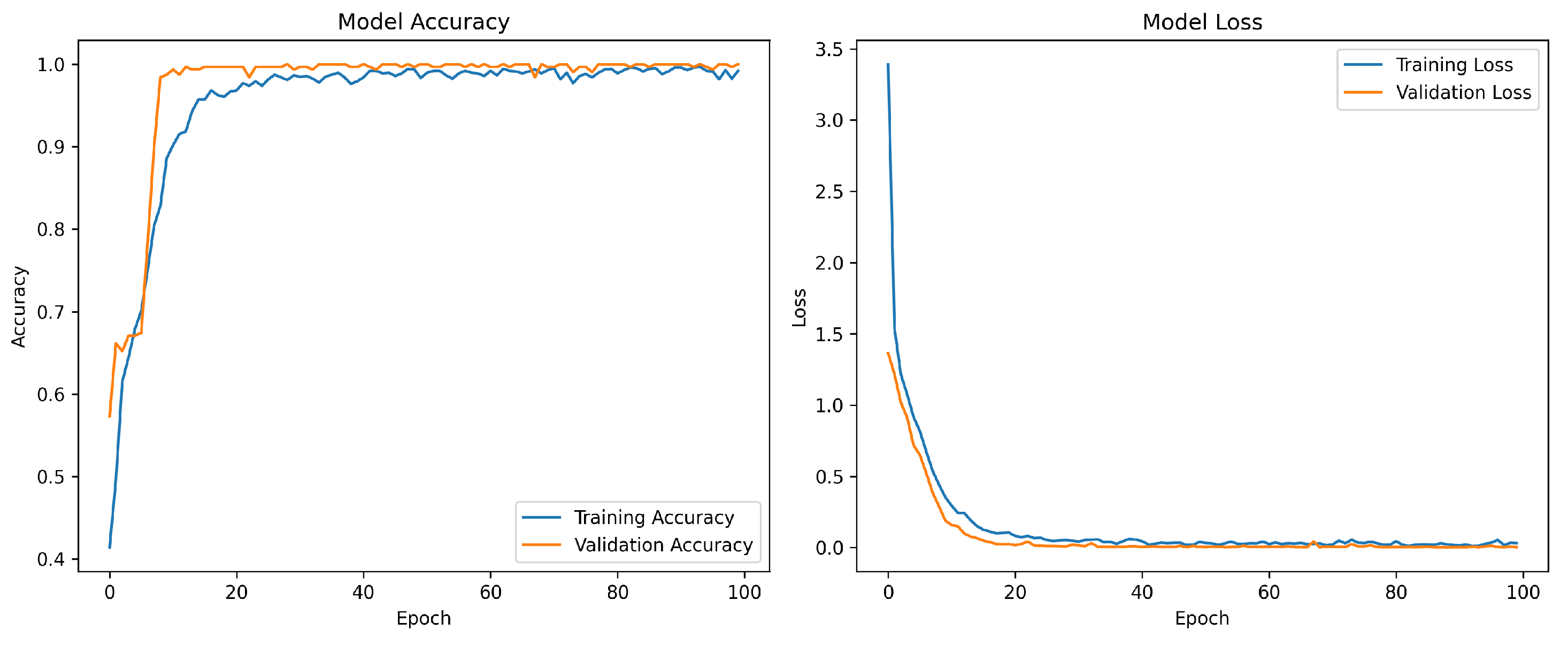
Figure 8.
Comparison of feature distribution between real and generated data.
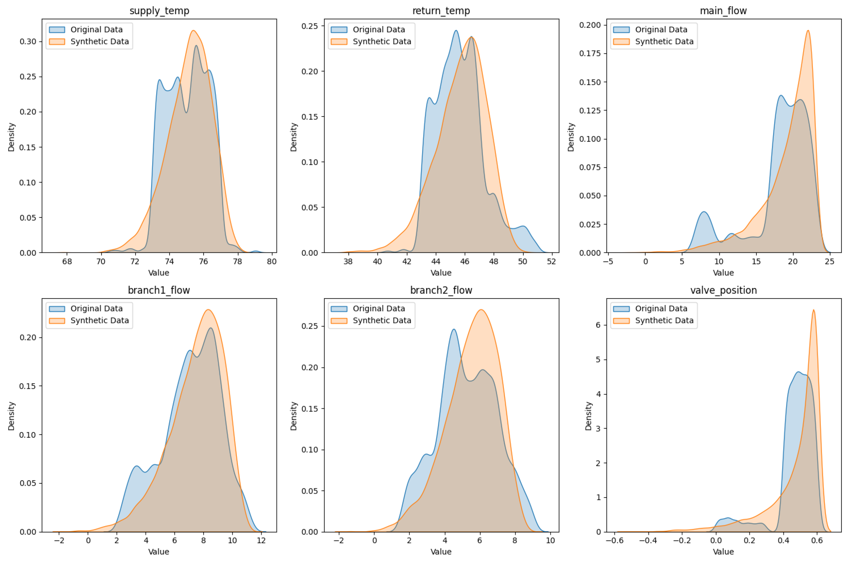
Figure 9.
Density distribution comparison of key parameters between real and generated data.
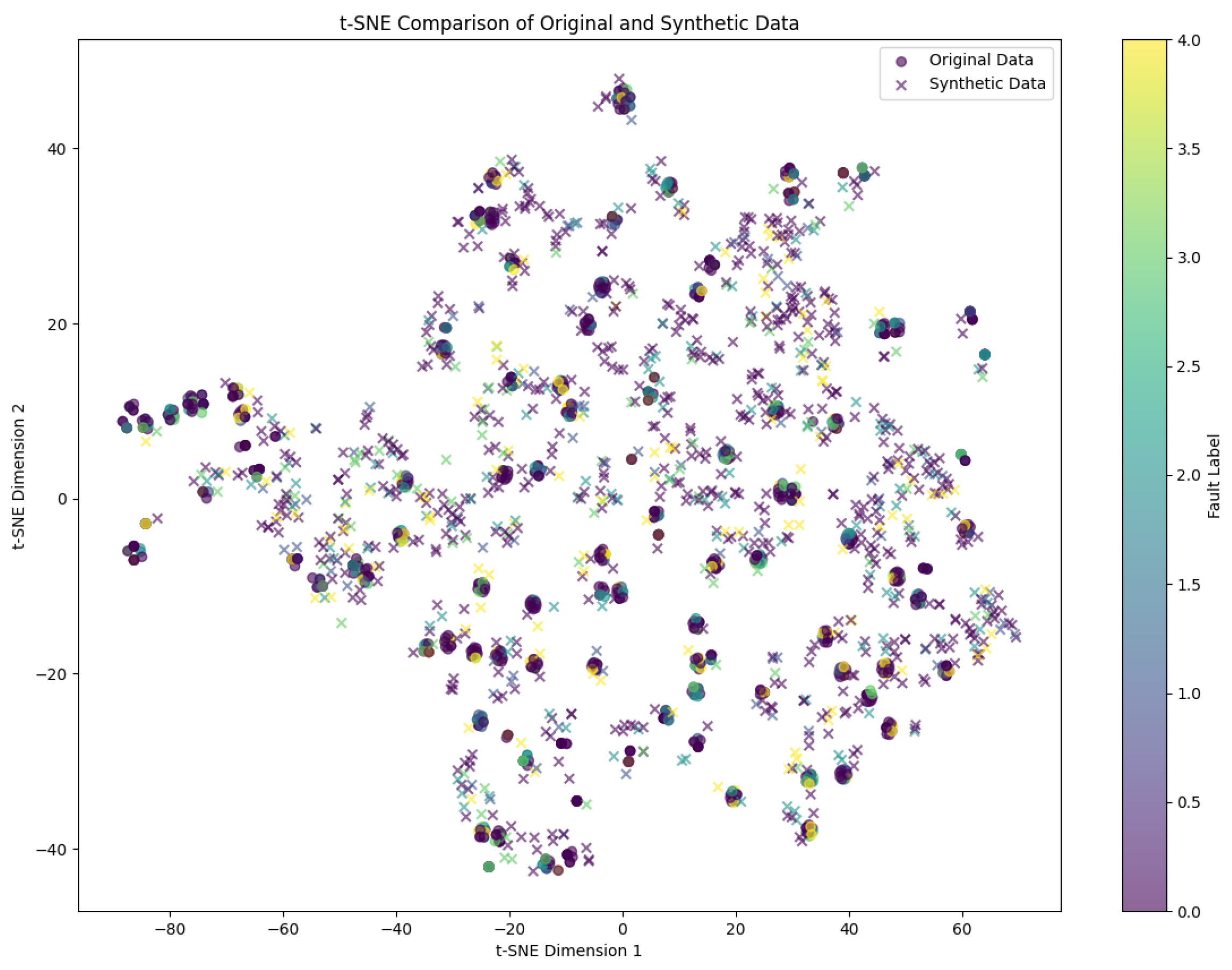
Figure 10.
Time series comparison between real and generated data.
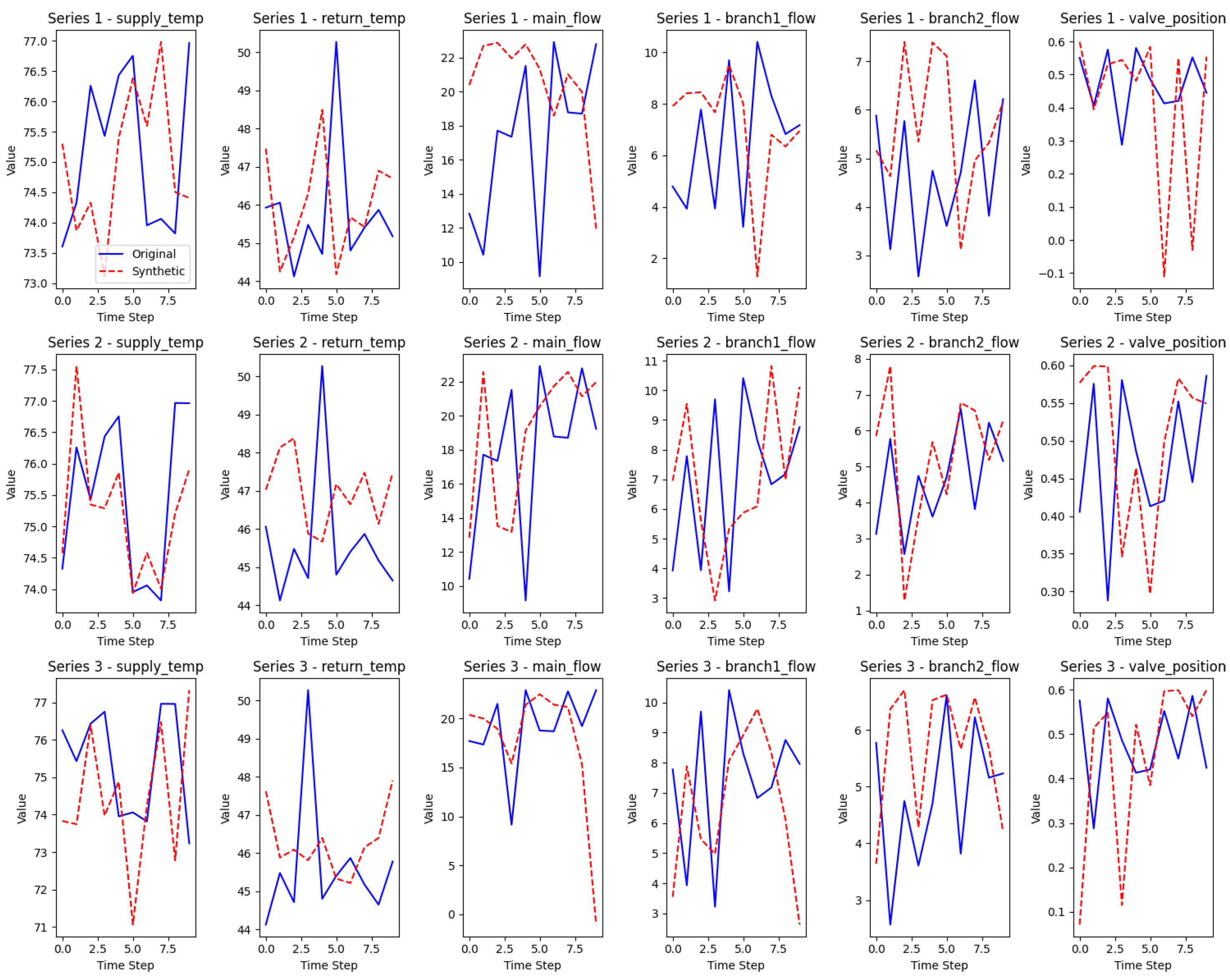

Table 1.
District Heating System Operating Parameters.
| Parameter Type | Baseline Value | Fluctuation Range | Unit | Physical Meaning |
|---|---|---|---|---|
| Supply Water Temp. | 75.0 | ±2.0 | °C | Heat source outlet water temperature |
| Return Water Temp. | 45.0 | ±2.0 | °C | User return water temperature |
| Main Pipe Flow Rate | 20.0 | ±3.0 | m³/h | Total system circulation volume |
| Valve Opening | 0.5 | ±0.1 | - | Flow regulation ratio |
| Branch A Ratio | 40% | ±10% | - | Building_A flow distribution |
| Branch B Ratio | 30% | ±30% | - | Building_B flow distribution |
Disclaimer/Publisher’s Note: The statements, opinions and data contained in all publications are solely those of the individual author(s) and contributor(s) and not of MDPI and/or the editor(s). MDPI and/or the editor(s) disclaim responsibility for any injury to people or property resulting from any ideas, methods, instructions or products referred to in the content. |
© 2025 by the authors. Licensee MDPI, Basel, Switzerland. This article is an open access article distributed under the terms and conditions of the Creative Commons Attribution (CC BY) license (http://creativecommons.org/licenses/by/4.0/).
Copyright: This open access article is published under a Creative Commons CC BY 4.0 license, which permit the free download, distribution, and reuse, provided that the author and preprint are cited in any reuse.


