
Submitted:
20 November 2025
Posted:
20 November 2025
You are already at the latest version
Abstract
Environmental monitoring systems generate large volumes of multivariate time series data from heterogeneous sensors, including those measuring soil, weather, and air quality parameters. However, sensor malfunctions and transmission failures frequently lead to missing values, compromising the performance of downstream analytical and predictive models. To address this challenge, this study extends a previously proposed hybrid architecture that interleaves Long Short-Term Memory (LSTM) layers with a Multi-Head Attention mechanism for robust multivariate data imputation. The first LSTM layer captures short-term temporal dependencies, the attention layer emphasizes long-range relationships among correlated features, and the second LSTM layer re-integrates these enriched representations into a coherent temporal sequence. The model is evaluated using multiple environmental datasets of soil temperature, meteorological (precipitation, temperature, wind speed, humidity), and air quality data across missingness levels ranging from 10% to 90%. Performance is compared against baseline methods including K-Nearest Neighbour (KNN) and Bidirectional Recurrent Imputation for Time Series (BRITS). An ablation study further examines the contribution of each layer to overall model performance. Results demonstrate that the proposed hybrid model achieves superior accuracy and robustness across datasets, confirming its effectiveness for environmental sensor data imputation under varying missing data conditions.
Keywords:
data imputation
; LSTM
; multihead attention
; missing data
; neural network
; time series
; environmental monitoring
1. Introduction
The rapid expansion of machine learning (ML) applications has dramatically increased the demand for large-scale, high-quality datasets that enable reliable and generalizable model training. The growing accessibility of cost-effective and scalable sensing technologies, such as Internet of Things (IoT) devices, remote sensing nodes, and wireless sensor networks has transformed how data are collected across domains. These systems continuously generate time-stamped data in areas ranging from healthcare monitoring and environmental systems to industrial automation and urban infrastructure, thereby providing a rich source of information for predictive modeling and decision support. However, this exponential increase in data acquisition also amplifies challenges related to data completeness, reliability, and consistency, which directly affect the robustness of ML-driven insights. In particular, data missingness has emerged as one of the most prevalent and detrimental issues, often arising from sensor drift, calibration errors, power failures, communication disruptions, or environmental interferences.
Missing or incomplete data is not confined to any single domain but appears across virtually all data-driven fields. It is particularly common in healthcare systems (Li et al. 2021; Wells et al. 2013; Zuo et al. 2021), geographic information systems (GIS) (Griffith and Liau 2021), transportation and traffic management (Kaur et al. 2022), environmental surveillance networks (Decorte et al. 2024; Okafor and Delaney 2021), and industrial process monitoring (Carbery et al. 2022). In these contexts, data gaps can lead to unreliable trend detection, erroneous forecasts, and reduced interpretability of analytical models. Furthermore, incomplete datasets can introduce statistical bias, distort model parameters, and reduce predictive accuracy when used in training or validation stages (Escobar et al. 2020; Hasan et al. 2021). These challenges are magnified in time-dependent domains, where data continuity and temporal correlations are essential for learning meaningful representations.
To mitigate the effects of missingness, two general strategies have been traditionally adopted, that are downsampling and imputation (Emran 2015). Downsampling eliminates incomplete observations entirely, simplifying analysis but at the cost of discarding potentially valuable information. This approach can be especially harmful in time series analysis, where removing data points disrupts temporal dependencies that are crucial for forecasting and anomaly detection (Okafor and Delaney 2021). In contrast, imputation methods attempt to estimate or reconstruct missing values using statistical inference, probabilistic reasoning, or machine learning-based modeling (Das et al. 2019). The effectiveness of an imputation approach depends not only on the chosen algorithm but also on the mechanism of missingness, which can be MCAR (Missing Completely at Random), MAR (Missing at Random), or MNAR (Missing Not at Random) (Brown and Kros 2003; Jäger et al. 2021; Kang 2013). Understanding this mechanism is vital for selecting appropriate techniques that minimize bias and preserve underlying data distributions.
Traditional imputation techniques are often categorized into Single Imputation (SI) and Multiple Imputation (MI) frameworks. SI approaches, including mean substitution, median filling, and zero imputation, offer simplicity and computational efficiency but tend to underestimate data variability and uncertainty (Kang 2013). MI, introduced through iterative modeling, generates multiple plausible versions of the complete dataset, capturing the inherent uncertainty in the imputation process (Jamshidian and Mata 2007). Classical statistical models such as regression, Expectation-Maximization (EM), and stochastic simulation have been widely used; however, their performance is typically limited when facing nonlinear or high-dimensional data structures (Brown and Kros 2003; Emmanuel et al. 2021). Consequently, recent years have witnessed a paradigm shift toward machine learning and deep learning-based solutions that can capture complex interdependencies among variables and temporal patterns.
A substantial body of research has benchmarked both conventional and learning-based imputation strategies across diverse applications. Kang (Kang 2013) surveyed traditional clinical data imputation methods such as Last Observation Carried Forward (LOCF), regression, and EM, while subsequent studies explored data-driven techniques including K-Nearest Neighbour (KNN), Random Forests (RF), Decision Trees (DT), Support Vector Machines (SVM) and ensemble learners (Emmanuel et al. 2021). Comparative analyses have demonstrated that model performance varies significantly with dataset characteristics and the type of missingness, suggesting there is no universal best method. For instance, Hegde et al. (Hegde et al. 2019) observed that Probabilistic Principal Component Analysis (PPCA) outperformed Multiple Imputation by Chained Equations (MICE) in healthcare datasets with MCAR missingness, while Stekhoven et al. (Stekhoven and Bühlmann 2012) showed that the non-parametric missForest algorithm achieved superior results on mixed-type biological datasets. Early neural network-based methods also demonstrated potential advantages: Gupta et al. (Gupta and Lam 1996) reported better results using backpropagation networks than with mean or regression imputation, and Silva-Ramírez et al. (Silva-Ramírez et al. 2011) validated multilayer perceptrons (MLPs) for robust imputation across both simulated and real-world datasets. More advanced models, such as deep autoencoders and variational autoencoders (VAEs), have since emerged as powerful tools capable of reconstructing complex patterns of missingness in nonlinear, high-dimensional spaces (Beaulieu-Jones and Moore 2017; McCoy et al. 2018).
With the rapid evolution of IoT infrastructures and real-time sensing systems, time series imputation has become a central research theme. Unlike cross-sectional data, time series are inherently sequential and temporally correlated, making traditional static imputation methods suboptimal. Decorte et al. (Decorte et al. 2024) investigated the performance of recurrent models such as Multi-Directional RNNs (M-RNN) and Bidirectional Recurrent Imputation for Time Series (BRITS) in environmental monitoring data with simulated MCAR conditions. Maksims et al. (Kazijevs and Samad 2023) benchmarked multiple deep learning architectures, including attention-based autoencoders, LSTM variants, and adversarial RNNs, across five healthcare datasets. Okafor and Delaney (Okafor and Delaney 2021) further demonstrated that variational autoencoder frameworks achieved superior reconstruction accuracy and improved calibration in greenhouse gas sensor networks when compared with traditional algorithms such as MICE, missForest, and KNN.
Recently, researchers have explored hybrid frameworks that integrate the strengths of deep sequential models with complementary algorithms. Examples include coupling Long Short-Term Memory (LSTM) networks with Decision Trees (Haibin and Yongliang 2023), optimizing learning with Genetic Algorithms (Tsoulos et al. 2024), or employing Transfer Learning strategies, for example, TrAdaBoost to handle domain adaptation challenges (Chen et al. 2021). Moreover, advances in attention mechanisms pioneered by transformer architectures in natural language processing (Domhan 2018; Strubell et al. 2018; Tang et al. 2018; Tao et al. 2018; Vaswani et al. 2017; Zhang and Thorburn 2021), have led to a surge of interest in attention-augmented imputation models. These models effectively learn context-aware temporal representations, capturing both short- and long-range dependencies within multivariate sequences.
Several studies and research experiments that have used hybrid methodologies to solve a variety of complex problems, particularly focusing on the innovative use of transformer mechanisms in conjunction with other neural network architectures, have greatly inspired us to explore further for imputing missing data in environmental datasets. A closely associated study conducted by Dagtekin et al. provides evidence that supports the potential efficacy of the combination of these techniques, as they present their findings of better imputation performance and prediction accuracy for water quality data through the integration of LSTM networks alongside self-attention mechanisms (Dagtekin and Dethlefs 2022). Similarly, Shang et al. have investigated the combination of LSTM, attention and AdaBoost algorithms to impute missing data in traffic flow dataset and have reported promising results (Shang et al. 2024).
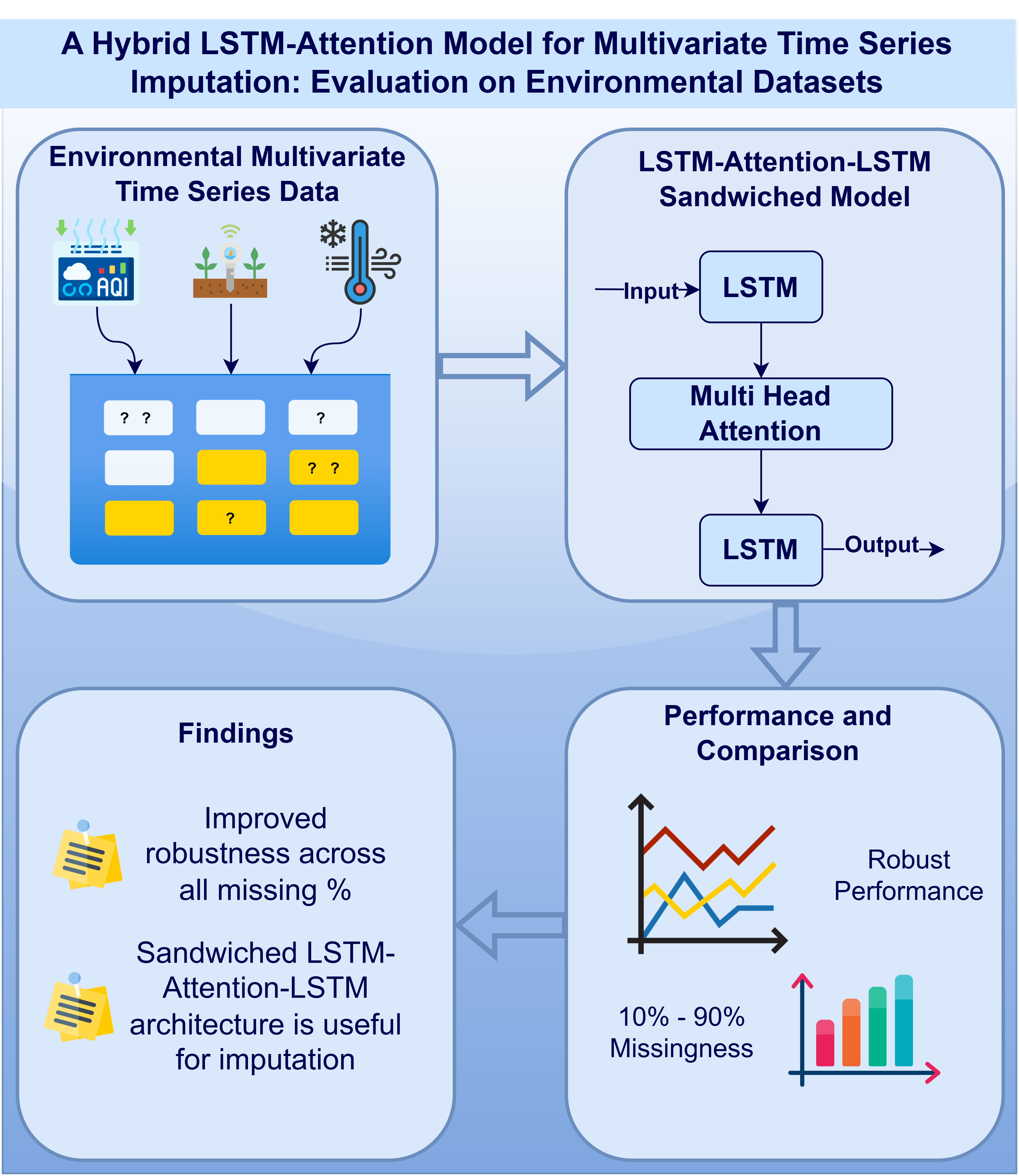
LSTM and attention hybrids are used extensively in NLP or healthcare but they are underexplored in environmental IoT monitroing. Secondly, many studies use attention mechanism either before or after the LSTM layer(s). In this paper, we present a hybrid LSTM-Attention model for missing data imputation in environmental monitoring datsets. We present a novel "sandwiched" LSTM - Attention - LSTM design. This interleaving enables the first LSTM layer to capture local temporal dependencies, the attention mechanism to highlight long-range relationships, and the second LSTM to re-integrate these enriched features into a coherent sequential representation. This ordering was deliberately chosen to balance sequential memory retention with global context modeling. Many prior works train models on complete data and then test performance on missing data. In our study, we trained the proposed model and other baseline models on 30% missing data to align it with real-world scenarios. We test imputation performance through MAE and RMSE across 10%-90% missingness, which provides a broad robustness analysis on low to moderate missingness. The proposed model demonstrates that it preserves accuracy under extreme missingness scenarios (70-80%), which is beneficial in real-world events of IoT sensor failures.
In the subsequent section of this paper, we briefly introduce the problem and highlight the purpose and significance of the work. The current state of the research in the problem domain is briefly reviewed and this section end with highlighting the contributions of this study. The next section described the proposed model in detail along with sufficient details of the data and mthodology adopted. Section 3 provides concise experimental results and their interpretations. The last section discusses the findings and their implications along with the limitations of the work. Future research directions are also mentioned in this section.
2. Materials and Methods
2.1. Dataset Description
To evaluate the performance and generalizability of the proposed hybrid model, multiple environmental monitoring datasets were used. These datasets represent varied sensing scenarios, including hydrological, meteorological, and air quality measurements collected from field-deployed sensor networks. Each dataset contains multivariate time series data with varying temporal resolutions, enabling a comprehensive assessment of the model’s imputation capabilities. For each dataset, the target variable, that is the feature to be predicted, is identified alongside a set of correlated auxilliary parameters that serve as input features. The relationships among these variables are visualized using correlation matrices, which help to illustrate the degree of association between the target and auxiliary features. Detailed descriptions of each dataset are provided in the following subsections.
2.1.1. Soil Temperature Dataset
The soil temperature dataset (SoilTemp) is a subset of the dataset originally published by (Decorte et al. 2024). This dataset comprises continuous time-series measurements of soil temperature recorded at three different heights using in-situ soil sensors proposed in (Wild et al. 2019). The sampling frequency for the sensor is 15 minutes in degrees Celsius, offering high temporal frequency and the time series spans 6 months of data observations from 19 April 2021 at 00:00:00 to 26 September 2021 at 23:45:00, providing a clearly defined study period.
The target feature in this dataset is the soil temperature measured at 12 cm above ground level named as in the dataset, as it exhibited the greatest variability among the three temperature sensors. The variability of the measurements makes it a suitable candidate for training and evaluating the proposed model, thereby enhancing the generalizability of the obtained results. Input features include soil temperature measurements at ground surface level (), subsurface soil temperature () 10 cm deep in the ground and relative humidity. The heatmap in Figure 1 shows the correlations between the target and input features. The heatmap inidcates strong correlation between the three temperature measurements, suggesting they can be useful predictors for the target feature. In comparison to this, a weak correlation between the traget feature and the relative humidity is present in the dataset. However, the target feature shows the strongest correlation with the humidity among the three temperature sensors.
2.1.2. Meteorological Dataset
The meteorological dataset is collected from an automatic weather station operating in the monitoring region under the SuDS+ project in Stanley, Durham, UK. The dataset contains records of nine different weather parameters at an hourly temporal resolution. The time series spans 16 months of data recorded from 11 June 2024 to 14 october 2025 to capture temporal patterns.
The target feature predicted in this dataset is the average air temperature measured in degrees Celsius which is a key climatic parameter. Other predictive features include average humidity, wind direction, wind speed, dew point, wind gust, heat index, wind chill and average rainfall in milimeters. As expected, temperature exhibits negative correlation with humidity and a strong positive correlation with heat index, dew point and wind chill parameters. The correlation matrix in Figure 2 highlights these relationships, which the proposed hybrid model leverages to improve the temporal estimation and imputation of air temperature values.
2.1.3. Air Quality Dataset
The air quality dataset utilized in this study is derived from the publicly available dataset presented by (Feinberg et al. 2018), hosted on the U.S. Environmental Protection Agency (EPA) Environmental Dataset Gateway (EDG EPA 2025). The dataset comprises measurements collected from low-cost gas sensors co-located with Federal Equivalent Method (FEM) reference monitors at an urban regulatory site in Denver, Colorado, USA. The monitoring period spanned approximately six months, from 8 September 2015 to 22 February 2016, with data aggregated at 15-minutes intervals.
Two target features are considered for analysis: ozone (O3) and combined nitrogen dioxide/ozone (NO2/O3) concentrations, both expressed in parts per billion (ppb). For both target features, measurements were obtained for corresponding temperature, relative humidity, and reference measurements from the FEM monitors. The gas sensors demonstrated moderate to strong correlations with other auxilliary features. Specifically, the correlation coefficients between O3 sensors and their reference exceeded 0.9, while those for NO2/O3 sensors ranged between 0.32 and 0.57. As illustrated in the correlation heatmap (Figure 3), the O3 sensors showed strong inter-sensor consistency and positive associations with temperature, alongside negative correlations with relative humidity. These relationships provide valuable contextual dependencies that the proposed hybrid model can exploit for accurate imputation and prediction of missing air quality measurements.
2.2. Proposed Hybrid Model
The hybrid model presented in this paper is a sequential neural network designed for time-series imputation tasks, using a combination of LSTM layers and a Multi-Head Attention mechanism to capture temporal dependencies and enhance feature representation. Figure 4 shows the overall architecture of the proposed model. The proposed architecture sandwiches the attention layer between the two LSTM layers instead of cascading the Attention and LSTM layers on top of each other. The model maps an input sequence to a scalar prediction via a first LSTM encoder producing hidden states . A multi-head self-attention module is then applied to , returning attention outputs . The concatenation of outputs from first LSTM and Attention layers is passed through a second LSTM, which re-encodes to produce the final hidden state . The output is obtained by a dense linear layer, and the network is trained by minimizing the mean squared error (MSE) as loss measure.
Before feeding the data into the model, missing values in the time series are reconstructed using linear interpolation to ensure temporal continuity. Given two observed data points and , the interpolated value at time t, where , is computed as
This method provides a simple yet effective way to fill small gaps in the data while preserving the temporal trend.
The interpolated data are subsequently normalized using Min-Max scaling to restrict all feature values within the range , which improves numerical stability and accelerates convergence during training. Each feature value is scaled as
where and represent the minimum and maximum values of the feature, respectively.
To capture sequential dependencies, feature engineering is applied using a sliding window technique with a window size of 30, denoted as T and represented by the parameter in this paper. Each input sample at time step t is expressed as
where , with for univariate data and for multivariate cases. This preprocessing pipeline ensures that the input sequences provided to the model are both complete and properly scaled, enabling effective learning of temporal relationships across multiple correlated features.
2.2.1. First LSTM Layer (LSTM1)
The preprocessed input is then passed to the first LSTM layer to learn long-term dependencies in sequential data (Hochreiter and Schmidhuber 1997). It utilizes 64 hidden units to learn local temporal dependencies and transforms the input sequence into a sequence of hidden states:
In our implementation, the standard hyperbolic tangent activation functions used in the candidate and output computations of the LSTM were replaced by ReLU to enhance gradient propagation and model stability. The overall LSTM formulation and gating mechanism remains consistent with the original definition by (Hochreiter and Schmidhuber 1997). Accordingly, the operations for the forget gate, input gate ,candidate state update and output gate are defined as the following equations.
where is the forget gate activation, and are the weight matrix and bias, is the previous hidden state, and is the input at any cuttrent time.
where is the input activation function result, and represents the candidate values to add to the cell state.
where ⊙ represents element-wise multiplication, is the output of forget gate, is the previous cell state, is the new input and is the new cell state.
where is the activation of the output gate, and is the new hidden state.
Hidden states produced at each time step are the output of this layer and are collected as
To mitigate overfitting, a Dropout layer is applied immediately after, with a dropout rate p selected as 0.3 to produce the following output.
2.2.2. Multihead Attention Layer
An Attention mechanism follows the initial LSTM layer to enhance feature representation by focusing on the most relevant parts of the sequence. The attention mechanism is a key element of transformer-based neural networks, enabling effective modeling of contextual dependencies. The multi-head attention variant extends this concept by projecting the input into multiple subspaces, one per head, to compute parallel attention scores that capture diverse contextual relationships within the sequence Vaswani et al. (2017). In the proposed model, six attention heads are used, with key vector dimensions equal to the LSTM output size, allowing the model to learn multiple attention patterns in parallel. For each attention head , queries, keys, and values are computed as:
where are learnable projection matrices and . The attention output for is computed through:
and outputs of all heads are concatenated and linearly projected to form the output .
To integrate global contextual information with local temporal patterns, the attention outputs and outputs from the first LSTM’s hidden states are concatenated at each time step:
2.2.3. Second LSTM Layer (LSTM2)
The concatenated sequence is then passed through a second LSTM layer with the same configurations as the :
This layer returns only the final hidden state , capturing high-level temporal representations. A Dropout layer similar to the first LSTM layer is applied at this stage too for additional regularization.
2.2.4. Output Layer
A final dense layer maps the final feature representation to the single scalar output which is then inverse-transformed to the original scale.
where and are trainable parameters, and denotes the linear activation function to predict the final value.
2.3. Experimental Design
This section outlines the methodological framework employed to evaluate the proposed hybrid deep learning model for missing data imputation. The experiments extend our previously published univariate results (Laeeq et al. 2026) by investigating the model’s performance on multivariate sensor datasets. The complete workflow includes missing data simulation, model training with cross-validation, and comparative evaluations against multiple baseline and ablation variants.
To systematically assess model performance, missing data were simulated on the target variable of each dataset using Bernoulli random sampling at a rate of 30%. The missing indices were generated randomly across the time steps to mimic realistic stochastic data loss in sensor networks. The auxiliary features remained complete and were used to support temporal and cross-variable correlations during imputation.
Each dataset was partitioned into training and test sets with a ratio of 80:20 without shuffling to preserve the temporal sequence. While the training data was further partitioned into training and validation sets to train the proposed hybrid model using 5-fold cross-validation, to ensure robustness and generalizability. Mean Squarred Error (MSE) was used as the loss measure during the training process. The best-performing model, as determined by validation loss, was then evaluated on unseen test data under varying levels of missingness from 10% to 90%. Performance was quantified using the Root Mean Squared Error (RMSE) and Mean Absolute Error (MAE), defined as:
where and denote the imputed and true values, respectively. These metrics were computed across all missingness levels to evaluate the model’s robustness under increasing data degradation.
The hybrid model is implemented using Python with open source libraries of Pandas, Numpy and TensorFlow. Table 1 summarizes the configuration and training parameters for the proposed model, used in all experiments.
The proposed model was benchmarked against two widely used imputation baselines: K-Nearest Neighbour (KNN) imputation, which estimates missing values based on the mean of the k most similar instances. For our experiments, we set k to be five.
BRITS (Bidirectional Recurrent Imputation for Time Series), a deep learning-based approach using bidirectional recurrent dynamics to model temporal dependencies. We used the for this model identical to for our proposed hybrid model. The was set to be 0.00001 and number of epochs used for each training fold was 50 for this model. These values are chosen to avoid zero training loss.
All comparative models were trained on the same datasets and evaluated using identical experimental conditions of 5-fold cross validation and performance metrics for fair comparison.
To investigate the contribution of each module within the hybrid model, three ablation variants were designed, as detailed in Table 2. Each variant omits or alters specific components to assess their impact on model performance. Each ablation model follows the same training and evaluation procedure as the full hybrid model. The resulting comparisons provide insights into the role of temporal sequencing and combining the outputs of LSTM and attention layer to b eused as input for the second LSTM layer, emphasizing the use of sandwich approach in the proposed model architecture.
3. Results
3.1. Multivariate Evaluation
Table 3 presents the MAE and RMSE values for four environmental datasets: SoilTemp, Meteorological, Air Quality NO2/O3, and Air Quality O3 across missingness levels ranging from 10% to 90%. Across all datasets, the model demonstrates strong robustness at lower levels of missingness, with relatively small changes in MAE and RMSE up to around 70%. Beyond this point, both metrics begin to rise more noticeably, and the degradation becomes substantial.
For the Soil Temperature dataset, the model exhibits the most stable behaviour. As shown in Table 3 and Figure 5(a), both MAE and RMSE remain nearly constant up to 70% missingness. A substantial increase is observed only beyond 80%, indicating that soil temperature values are easier to reconstruct even when a large portion of data is missing. The Meteorological dataset displays similarly consistent performance at moderate missingness levels. Interestingly, MAE slightly improves up to 40%, however, Figure 5(b) show a clear increase in both metrics once missingness exceeds 60%, with a sharp rise at 80-90%. In the Air Quality NO2/O3 dataset, the model maintains stability up to approximately 40% missingness, but errors increase steadily after that. As illustrated in Figure 5(c), MAE nearly doubles between 10% and 90%, reflecting the higher variability and nonlinearity typically associated with air pollutant dynamics. Finally, the Air Quality O3 dataset shows small absolute error values due to its lower numerical range, but the upward trend with increasing missingness is still evident (Figure 5(d)). While errors remain minimal up to 60%, both MAE and RMSE rise consistently beyond 60%, confirming that even low-magnitude datasets eventually exhibit degradation as missingness becomes severe.
Overall, the results show that the model performs reliably under moderate to high missingness conditions for all environmental datasets, but predictable degradation occurs at extreme levels of missing data.
3.2. Comparative Study
Table 4 reports the Mean Absolute Error (MAE) comparison and Table 5 shows the corresponding RMSE values for the Hybrid model, KNN and BRITS across four environmental datasets and missingness levels from 10% to 90%. Visual comparison is available in Figure 6 and Figure 7.
For the SoilTemp dataset, the proposed hybrid model consistently achieves the lowest MAE and RMSE across most missingness levels, demonstrating strong robustness to data loss. For example, at 30% missingness the Hybrid MAE is 0.0962 while KNN and BRITS record 0.4045 and 0.5733, respectively; the RMSE trend is also similar. These differences are clearly visible in Figure 6(a) and Figure 7(a).
The Meteorological dataset exhibits a different pattern, KNN outperforms the Hybrid model across the reported missingness levels. However, the RMSE results (Table 5 and Figure 7(b)) provides a more interesting picture. The Hybrid model attains slightly lower RMSE than KNN at low to moderate missingness, indicating that although KNN gives smaller average absolute errors, the Hybrid produces fewer very large errors in these missingness levels. At higher missingness (80-90%) KNN’s RMSE becomes lower than Hybrid’s, reflecting KNN’s relative resilience in reducing large residuals for this dataset at extreme data loss. These contrasting MAE/RMSE behaviours suggest that for Meteorological data KNN yields smaller average deviations while the Hybrid reduces large errors at low-to-moderate missingness.
For the NO2/O3 target, KNN initially achieves lower MAE than the Hybrid at low missingness; as presented in Table 4 and Figure 6(c). However, this advantage diminishes as missingness increases, and the Hybrid overtakes KNN from roughly 50% missingness onward. The RMSE series shows that Hybrid already attains lower RMSE than KNN from as early as 20% missingness, indicating that the Hybrid is better at limiting larger errors even when KNN has lower MAE at the very lowest missingness levels. In short, KNN is initially better on MAE for NO2/O3, but Hybrid becomes superior as missingness grows; RMSE shows the Hybrid reduces large residuals earlier than MAE suggests. For O3, absolute errors are very small for all methods; nevertheless, the Hybrid maintains a small but consistent advantage in MAE across most missingness levels and RMSE values follow the same pattern.
3.3. Ablation Study
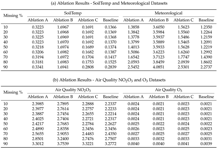
Ablation study was conducted to evaluate the performance of three ablation variants (A, B, C) as defined in Table 2 against the proposed hybrid baseline model across four datasets (SoilTemp, Meteorological, Air Quality NO2O3, and Air Quality O3) using MAE and RMSE metrics under varying missing data percentages (10%-90%). The results of this study for all four datasets are summarised in Table 6 and Table 7 and a visual representation is created in Figure 8 and Figure 9.
For SoilTemp dataset, across all missingness levels, the Baseline achieves the lowest MAE and RMSE, confirming that the full hybrid structure is essential for accurate reconstruction. Ablation B performs the worst, with very large errors at all missingness levels, indicating that the LSTM component is critical for capturing temporal dependencies. Ablation A and Ablation C perform moderately but consistently worse than the Baseline. RMSE results in Table 7 and Figure 9(a) follow the same trend, reinforcing the dominance of the Baseline model.
A similar pattern is observed in the Meteorological dataset. Ablation B again yields extremely high error values across all missingness levels (Table 6 and Figure 8(b)), showing that temporal modeling is indispensable for meteorological dataset as well. Ablation A and Ablation C remain competitive with each other but remain consistently inferior to the Baseline. RMSE comparisons reflect the same ordering. The Baseline retains a clear advantage across all missingness levels.
For the NO2/O3 dataset, the Baseline again outperforms all ablated variants across both metrics. Ablation B remains the poorest performer (MAE increasing to 3.3611 at 90%), while Ablation A and Ablation C track more closely. Notably, Ablation C performs relatively closer to the Baseline at very low missingness (10%) but diverges at higher missingness. RMSE differences in Table 7 and Figure 9(c) show a sharper degradation for all ablations, with Ablation B exhibiting the steepest rise.
The O3 dataset exhibits very small absolute error magnitudes, but the relative behaviour remains consistent with the other datasets. The Baseline consistently achieves the best MAE and RMSE values. At low missingness levels, Ablation A and Ablation C perform comparably to the Baseline, but Ablation B again shows noticeably higher errors. The RMSE curves in Figure 9(d) show similarly small but consistent gaps.
4. Discussion
The results of the multivariate evaluation of the proposed hybrid model demonstrate that it provides reliable imputation performance across diverse environmental datasets, maintaining stable MAE and RMSE values up to approximately 40-70% missingness. This robustness indicates that the architecture effectively captures temporal dependencies, allowing it to reconstruct missing patterns even when substantial portions of the sequence are absent. However, the sharp increase in error beyond 70-80% missingness highlights the limitations of the model when the available contextual information becomes insufficient. Air quality datasets, particularly NO2/O3, show more rapid deterioration due to their higher variability, whereas Soil Temperature remains stable for longer. These findings underscore that while the model is well-suited for real-world environmental monitoring scenarios with moderate to high data loss, extreme missingness still presents a significant challenge that future work should address through enhanced temporal reasoning or external information integration.
The comparative evaluation highlights the strong performance and robustness of the proposed Hybrid model relative to KNN and BRITS across the four environmental datasets. In the SoilTemp and O3 datasets, the Hybrid model consistently yields the lowest errors, even under extreme missingness. These datasets exhibit smoother temporal variations, enabling the Hybrid model to effectively leverage both local feature extraction and sequence learning to reconstruct missing values with high stability.
In the Meteorological dataset, however, KNN demonstrates competitive behaviour at low missingness levels, marginally outperforming the Hybrid model in both MAE and RMSE. This result suggests that meteorological variables contain short-range correlations that KNN can exploit effectively through distance-based interpolation. Figure 10 shows the distribution comparison of and , target features in SoilTemp and Meteorological daatsets respectively. may show skewness, reflecting localized fluctuations, while, distribution is smoother and less skewed, indicating stability from averaging. exhibits a wider range, suggesting more variability in sensor readings. On the other hand, is more concentratedand hence neigbouring values are favouring imputation. As missingness increases, KNN’s neighbourhood becomes sparse, and its performance deteriorates, allowing the Hybrid model to surpass it. This behaviour illustrates the advantage of Hybrid’s architecture in maintaining reconstruction accuracy under progressively degraded information availability.
A similar pattern emerges in the NO2/O3 dataset, where KNN initially achieves lower error metrics than the Hybrid model at 10-30% missingness. Pollutant concentrations often exhibit strong local covariation, explaining KNN’s effectiveness in early stages. However, as the missingness grows, the Hybrid model becomes the most accurate method, consistently outperforming both KNN and BRITS. The rapid performance decline of BRITS across all datasets and missingness levels indicates that, despite being designed for irregular time series, it struggles to maintain stability under the types of data gaps and nonlinear dynamics present in environmental monitoring.
Overall, the comparative study shows that the Hybrid model generalises more effectively than KNN and BRITS across diverse environmental datasets, particularly when missingness becomes substantial. Its ability to integrate local, sequential, and contextual information enables strong performance.
The ablation study confirms that each component of the Hybrid model; multihead attention and the two LSTM temporal modules contribute positively to reconstruction accuracy. The Baseline consistently achieves the lowest MAE and RMSE values and shows the most stable behaviour across all missingness levels. These results validate the necessity of the full hybrid design and highlight the complementary strengths of its constituent components. Across datasets and metrics, Ablation B (removal of the second LSTM) is the most detrimental modification. The consistently poor performance of Ablation B across SoilTemp, Meteorological and NO2/O3 datasets demonstrates that the post-attention sequence module (LSTM2) is critical for producing accurate reconstructions when attention outputs are to be re-integrated into a sequential representation.
Ablation A (removal of the first / pre-attention LSTM) and Ablation C (removal of the attention mechanism) both produce moderate degradations relative to the Baseline but do not cause the extreme failure observed for Ablation B. For NO2/O3, Ablation C is relatively close to the Baseline at low missingness (MAE 1.7326 vs. Baseline 1.6996 at 10%), but its error grows faster with increasing missingness (see Figure 8(c)), indicating that attention contributes increasingly with larger data gaps. The O3 target (small-magnitude values) reflects the same qualitative pattern but with much smaller absolute errors: the Baseline maintains the best MAE/RMSE across missingness levels and Ablation B again produces the largest deterioration.
In summary, Removing the post-attention LSTM (Ablation B) causes the largest and most consistent performance drop across datasets and metrics, highlighting the importance of re-integrating attention-enhanced features into the sequential model. Omitting the pre-attention LSTM (Ablation A) or the attention module (Ablation C) leads to moderate but measurable degradations; attention becomes progressively more important as missingness increases. The full Baseline configuration consistently attains the lowest MAE and RMSE values, confirming that the combined sandwiched pipeline (LSTM1 + Attention + LSTM2) provides the most reliable reconstruction performance under varying degrees of data loss and varying types of data distributions.
Future research directions include hyperparameter optimisation and imputing a sequence of missing values as an output of this model. Understanding the inference of the model by analysing the attention weights to see what feature are important in making imputations and what time steps are more significant thatn others can be another future direction. Testing the model on datasets from other domains can be a useful way forward in evaluating the generalisability and robustness of the proposed model.
5. Conclusions
In this study, we presented a hybrid deep learning framework for robust missing data imputation in environmental monitoring datasets. By integrating LSTM with attention mechanism, in sandwiched interleaved manner, our model effectively captures both temporal and spatial dependencies, outperforming baseline and ablation variants in terms of MAE and RMSE. The results demonstrate that the proposed approach not only enhances imputation accuracy under varying levels of missingness but also maintains stability across different environmental datasets. These findings highlight the potential of hybrid architectures for improving data quality in environmental monitoring systems, which is critical for reliable decision-making and downstream tasks.
Author Contributions
Funding acquisition, U.A. and J.L.; supervision, U.A. and J.L.; methodology, J.L., A.L., and U.A.; implementation, A.L.; writing—original draft preparation, A.L., U.A., and J.L.; writing—review and editing, A.L., U.A., and J.L. All authors have read and agreed to the published version of the manuscript.
Funding
This work has been funded by the research project "Community SuDS Innovation Accelerator", as part of the Flood and Coastal Resilience Innovation Programme (FCRIP) by Environmental Agency (EA), UK.
Institutional Review Board Statement
Not applicable.
Informed Consent Statement
Not applicable.
Data Availability Statement
The data used and source code developed to reproduce the results of this study have been made publicly available on GitHub and can be accessed at the following repository: https://github.com/ammara-tees/LSTM-attention-model (accessed on 18 November 2025).
Conflicts of Interest
The authors declare no conflicts of interest.
References
- Beaulieu-Jones, Brett K. and Jason H. Moore. 2017. Missing data imputation in the electronic health record using deeply learned autoencoders. In Proceedings of the Pacific Symposium on Biocomputing, Volume 22, pp. 207–218.
- Brown, Marvin and John Kros. 2003. Data mining and the impact of missing data. Industrial Management and Data Systems 103, 611–621. [CrossRef]
- Carbery, Caoimhe M., Roger Woods, Cormac McAteer, and David M. Ferguson. 2022. Missingness analysis of manufacturing systems: a case study. Proceedings of the Institution of Mechanical Engineers 236(10), 1406–1417. [CrossRef]
- Chen, Zeng, Huan Xu, Peng Jiang, Shanen Yu, Guang Lin, Igor Bychkov, Alexey Hmelnov, Gennady Ruzhnikov, Ning Zhu, and Zhen Liu. 2021. A transfer learning-based lstm strategy for imputing large-scale consecutive missing data and its application in a water quality prediction system. Journal of Hydrology 602, 126573. [CrossRef]
- Dagtekin, Onatkut and Nina Dethlefs. 2022. Imputation of partially observed water quality data using self-attention lstm. In 2022 International Joint Conference on Neural Networks (IJCNN), pp. 1–8.
- Das, Dipalika, Maya Nayak, and Subhendu Pani. 2019. Missing value imputation—a review. International Journal of Computer Sciences and Engineering 7, 548–558. [CrossRef]
- Decorte, Thomas, Steven Mortier, Jonas J. Lembrechts, Filip J. R. Meysman, Steven Latré, Erik Mannens, and Tim Verdonck. 2024. Missing value imputation of wireless sensor data for environmental monitoring. Sensors 24(8). [CrossRef]
- Domhan, Tobias. 2018. How much attention do you need? a granular analysis of neural machine translation architectures. In Proceedings of the 56th Annual Meeting of the Association for Computational Linguistics (Volume 1: Long Papers), Volume 1, pp. 1799–1808.
- EDG EPA. 2025. Epa environmental dataset gateway. Accessed: Nov. 11, 2025.
- Emmanuel, Tlamelo, Thabiso Maupong, Dimane Mpoeleng, Thabo Semong, Banyatsang Mphago, and Oteng Tabona. 2021. A survey on missing data in machine learning. Journal of Big Data 8(140). [CrossRef]
- Emran, Nurul A. 2015. Data completeness measures. In A. Abraham, A. K. Muda, and Y.-H. Choo (Eds.), Pattern Analysis, Intelligent Security and the Internet of Things, pp. 117–130. Cham: Springer International Publishing.
- Escobar, Carlos, Jorge Arinez, Daniela Macias, and Ruben Morales-Menendez. 2020. Learning with missing data. In IEEE International Conference on Big Data (Big Data).
- Feinberg, S., R. Williams, G. S. W. Hagler, J. Rickard, R. Brown, D. Garver, G. Harshfield, P. Stauffer, E. Mattson, R. Judge, and S. Garvey. 2018. Long-term evaluation of air sensor technology under ambient conditions in denver, colorado. Atmospheric Measurement Techniques 11(8), 4605–4615. [CrossRef]
- Griffith, Daniel A. and Yan-Ting Liau. 2021. Imputed spatial data: cautions arising from response and covariate imputation measurement error. Spatial Statistics 42, 100419. [CrossRef]
- Gupta, Amit and Monica S. Lam. 1996. Estimating missing values using neural networks. The Journal of the Operational Research Society 47(2), 229–238.
- Haibin, Chen and Huang Yongliang. 2023. A hybrid lstm and decision tree model: a novel machine learning architecture for complex data classification. In IEEE International Conference on Sensors, Electronics and Computer Engineering (ICSECE), pp. 1441–1446.
- Hasan, Md. Kamrul, Md. Ashraful Alam, Shidhartho Roy, Aishwariya Dutta, Md. Tasnim Jawad, and Sunanda Das. 2021. Missing value imputation affects the performance of machine learning: a review and analysis of the literature (2010–2021). Informatics in Medicine Unlocked 27, 100799. [CrossRef]
- Hegde, Harshad, Neel Shimpi, Aloksagar Panny, Ingrid Glurich, Pamela Christie, and Amit Acharya. 2019. Mice vs ppca: missing data imputation in healthcare. Informatics in Medicine Unlocked 17, 100275. [CrossRef]
- Hochreiter, Sepp and Jürgen Schmidhuber. 1997. Long short-term memory. Neural Computation 9(8), 1735–1780.
- Jamshidian, Mortaza and Matthew Mata. 2007. Advances in analysis of mean and covariance structure when data are incomplete. In Handbook of Latent Variable and Related Models, pp. 21–44. North-Holland.
- Jäger, Sebastian, Arndt Allhorn, and Felix Bießmann. 2021. A benchmark for data imputation methods. Frontiers in Big Data 4. [CrossRef]
- Kang, Hyun. 2013. The prevention and handling of the missing data. Korean Journal of Anesthesiology 64(5), 402–406. [CrossRef]
- Kaur, Mankirat, Sarbjeet Singh, and Naveen Aggarwal. 2022. Missing traffic data imputation using a dual-stage error-corrected boosting regressor with uncertainty estimation. Information Sciences 586, 344–373. [CrossRef]
- Kazijevs, Maksims and Manar D. Samad. 2023. Deep imputation of missing values in time series health data: a review with benchmarking. Journal of Biomedical Informatics 144, 104440. [CrossRef]
- Laeeq, Ammara, Usman Adeel, Jie Li, and Eleanor Starkey. 2026. A hybrid lstm-attention approach for missing data imputation in iot time series. In Intelligent Data Engineering and Automated Learning – IDEAL 2025, pp. 301–312. Springer Nature Switzerland.
- Li, J., X. S. Yan, D. Chaudhary, V. Avula, S. Mudiganti, H. Husby, S. Shahjouei, A. Afshar, W. F. Stewart, M. Yeasin, R. Zand, and V. Abedi. 2021. Imputation of missing values for electronic health record laboratory data. npj Digital Medicine 4(1), 147. [CrossRef]
- McCoy, John T., Steve Kroon, and Lidia Auret. 2018. Variational autoencoders for missing data imputation with application to a simulated milling circuit. IFAC-PapersOnLine 51(21), 141–146. [CrossRef]
- Okafor, Nwamaka U. and Declan T. Delaney. 2021. Missing data imputation on iot sensor networks: implications for on-site sensor calibration. IEEE Sensors Journal 21(20), 22833–22845. [CrossRef]
- Shang, Qian, Yujie Tang, and Liang Yin. 2024. A hybrid model for missing traffic flow data imputation based on clustering and attention mechanism optimizing lstm and adaboost. Scientific Reports 14, 26473.
- Silva-Ramírez, Esther-Lydia, Rafael Pino-Mejías, Manuel López-Coello, and María-Dolores Cubiles-de-la Vega. 2011. Missing value imputation on missing completely at random data using multilayer perceptrons. Neural Networks 24(1), 121–129. [CrossRef]
- Stekhoven, Daniel and Peter Bühlmann. 2012. Missforest: non-parametric missing value imputation for mixed-type data. Bioinformatics (Oxford, England) 28, 112–118. [CrossRef]
- Strubell, Emma, Patrick Verga, Daniel Andor, David Weiss, and Andrew McCallum. 2018. Linguistically-informed self-attention for semantic role labeling. In Proceedings of the 2018 Conference on Empirical Methods in Natural Language Processing, pp. 5027–5038. Association for Computational Linguistics.
- Tang, Gongbo, Mathias Müller, Annette Rios, and Rico Sennrich. 2018. Why self-attention? a targeted evaluation of neural machine translation architectures. In Proceedings of the 2018 Conference on Empirical Methods in Natural Language Processing, pp. 4263–4272. Association for Computational Linguistics.
- Tao, Chongyang, Shen Gao, Mingyue Shang, Wei Wu, Dongyan Zhao, and Rui Yan. 2018. Get the point of my utterance! learning towards effective responses with multi-head attention mechanism. In Proceedings of the Twenty-Seventh International Joint Conference on Artificial Intelligence (IJCAI-18), pp. 4418–4424. International Joint Conferences on Artificial Intelligence Organization.
- Tsoulos, Ioannis, Vasilis Charilogis, and Dimitrios Tsalikakis. 2024. Train neural networks with a hybrid method that incorporates a novel simulated annealing procedure. AppliedMath 4, 1143–1161. [CrossRef]
- Vaswani, Ashish, Noam Shazeer, Niki Parmar, Jakob Uszkoreit, Llion Jones, Aidan N. Gomez, Łukasz Kaiser, and Illia Polosukhin. 2017. Attention is all you need. In Advances in Neural Information Processing Systems, Volume 30, pp. 5998–6008. Curran Associates, Inc.
- Wells, Brian, Amy Nowacki, Kevin Chagin, and Michael Kattan. 2013. Strategies for handling missing data in electronic health record derived data. Generating Evidence and Methods to Improve Patient Outcomes (eGEMs) 1. [CrossRef]
- Wild, Jan, Martin Kopecký, Martin Macek, Martin Šanda, Jakub Jankovec, and Tomáš Haase. 2019. Climate at ecologically relevant scales: A new temperature and soil moisture logger for long-term microclimate measurement. Agricultural and Forest Meteorology 268, 40–47. [CrossRef]
- Zhang, Yifan and Peter J. Thorburn. 2021. A dual-head attention model for time series data imputation. Computers and Electronics in Agriculture 189, 106377. [CrossRef]
- Zuo, Zheming, Jie Li, Han Xu, and Noura Al Moubayed. 2021. Curvature-based feature selection with application in classifying electronic health records. Technological Forecasting and Social Change 173, 121127. [CrossRef]
Figure 1.
Correlation matrix of the features in the SoilTemp dataset.
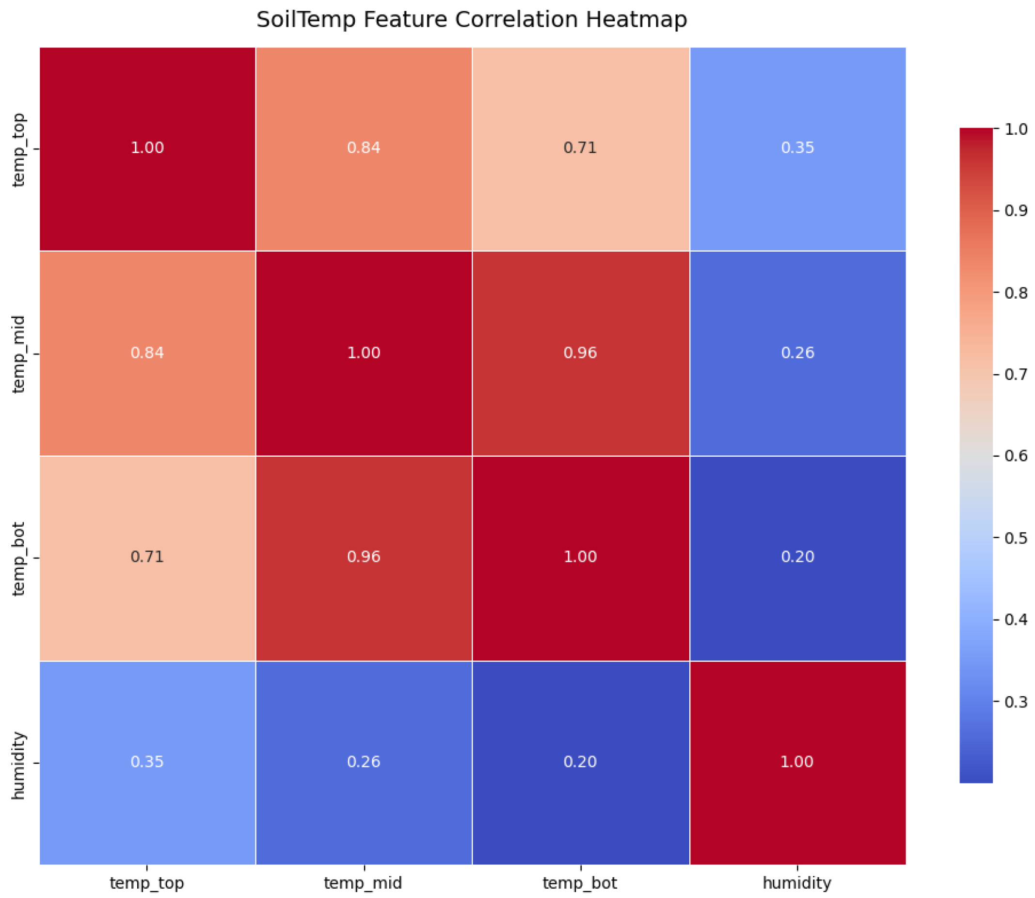
Figure 2.
Correlation matrix of the features in the Meteorological dataset.
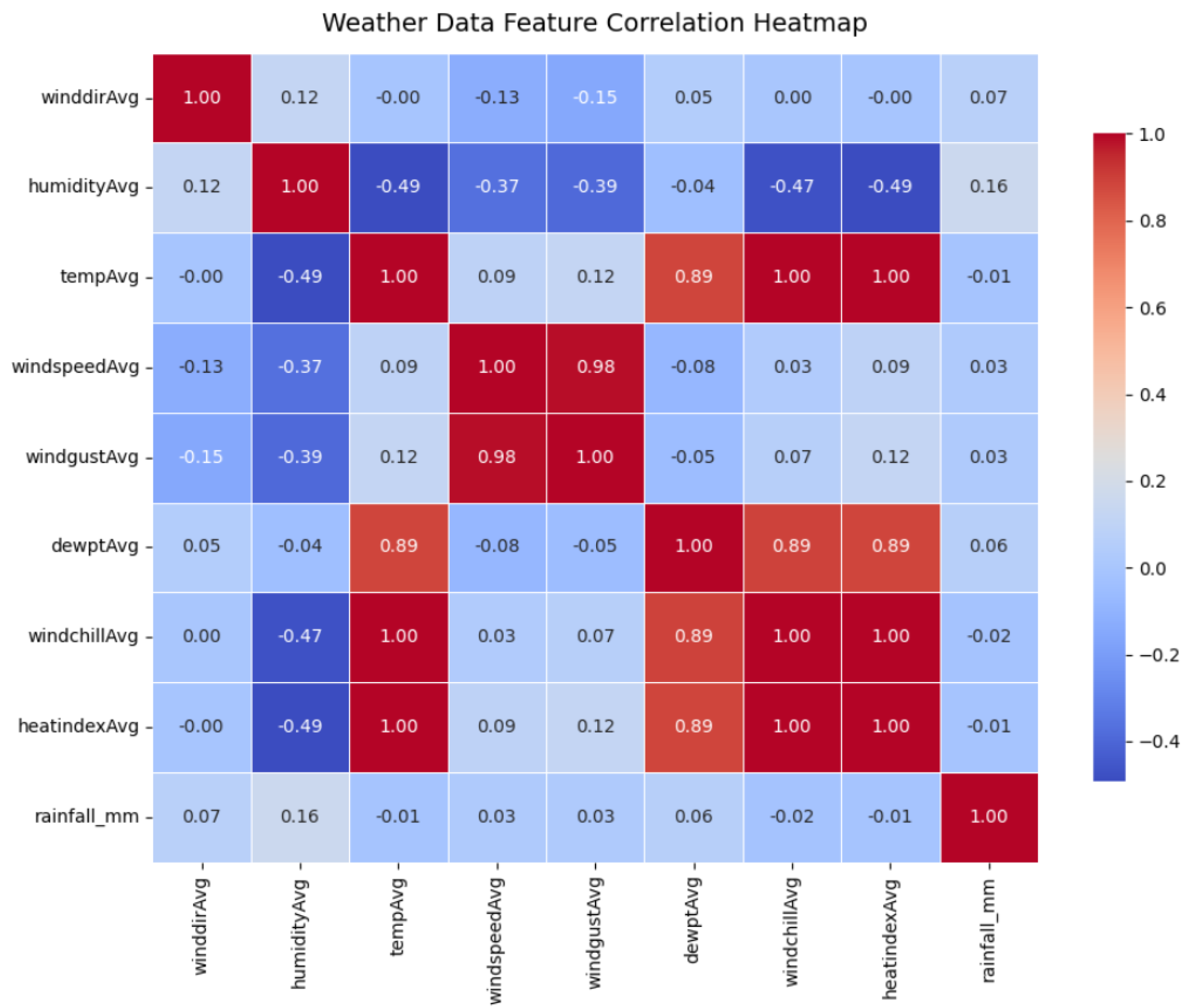
Figure 3.
(a) Correlation matrix of the features in the NO2/O3 dataset. (b) Correlation matrix of the features in the O3 dataset.
Figure 3.
(a) Correlation matrix of the features in the NO2/O3 dataset. (b) Correlation matrix of the features in the O3 dataset.
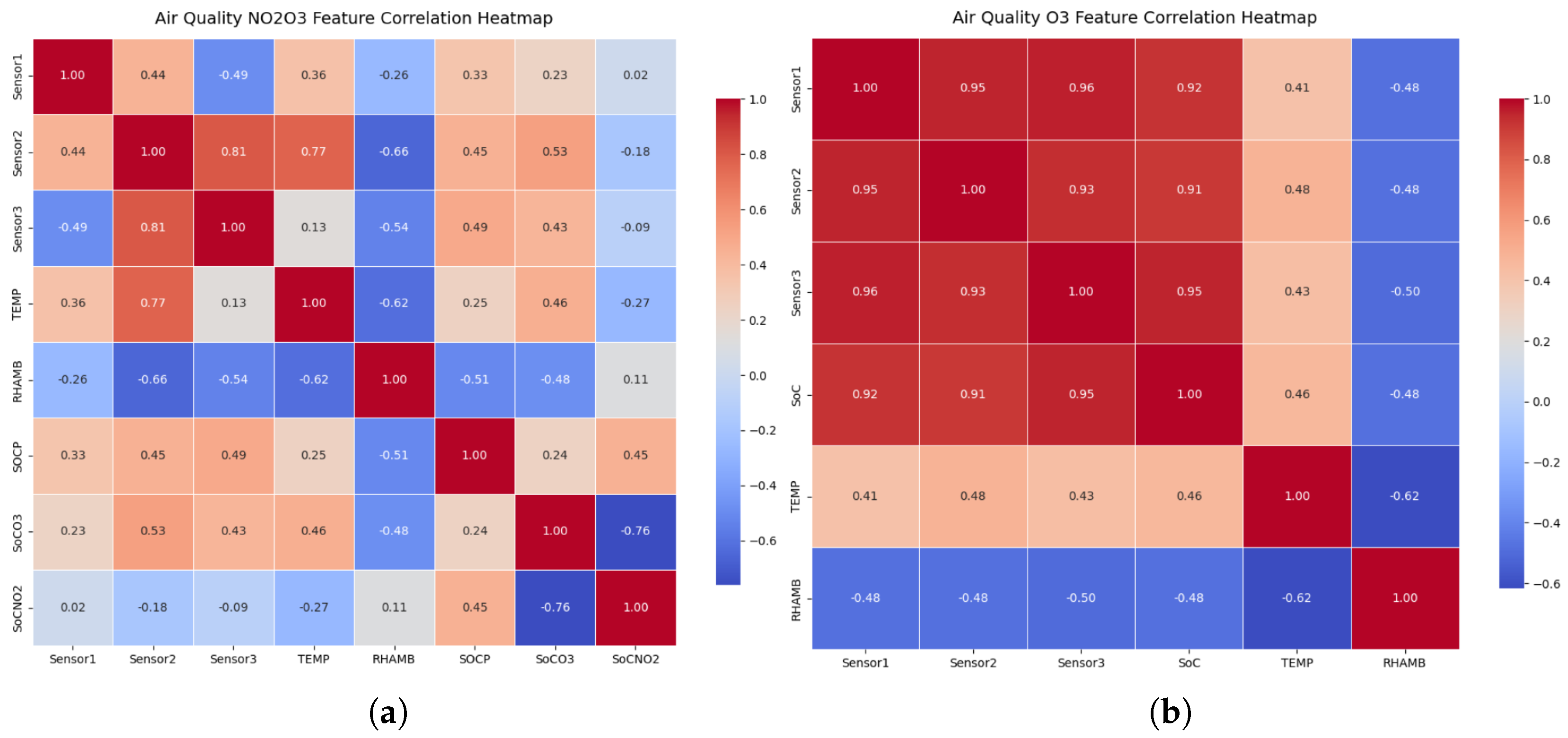
Figure 4.
Proposed Hybrid Model Archotecture.

Figure 5.
MAE and RMSE trends across increasing missingness levels for (a) SoilTemp, (b) Meteorological, (c) Air Quality NO2/O3, and (d) Air Quality O3 datasets.
Figure 5.
MAE and RMSE trends across increasing missingness levels for (a) SoilTemp, (b) Meteorological, (c) Air Quality NO2/O3, and (d) Air Quality O3 datasets.
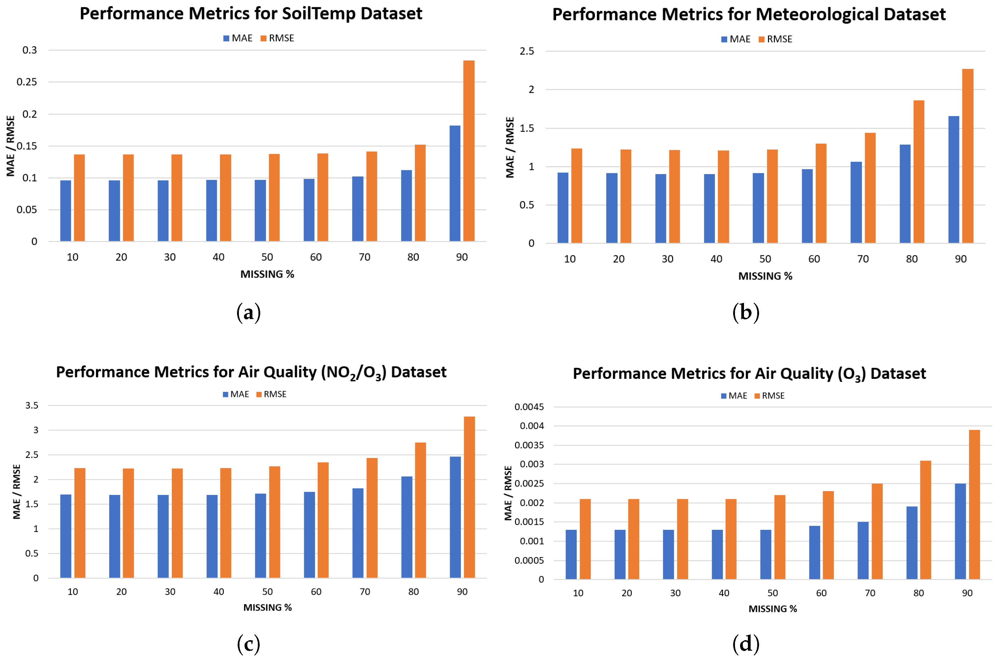
Figure 6.
Mean Absolute Error (MAE) comparison of the Hybrid model, KNN, and BRITS across different levels of induced missingness for (a) SoilTemp, (b) Meteorological, (c) Air Quality NO2/O3, and (d) Air Quality O3 datasets.
Figure 6.
Mean Absolute Error (MAE) comparison of the Hybrid model, KNN, and BRITS across different levels of induced missingness for (a) SoilTemp, (b) Meteorological, (c) Air Quality NO2/O3, and (d) Air Quality O3 datasets.

Figure 7.
Root Mean Squared Error (RMSE) comparison of the Hybrid model, KNN, and BRITS across different levels of induced missingness for (a) SoilTemp, (b) Meteorological, (c) Air Quality NO2/O3, and (d) Air Quality O3 datasets.
Figure 7.
Root Mean Squared Error (RMSE) comparison of the Hybrid model, KNN, and BRITS across different levels of induced missingness for (a) SoilTemp, (b) Meteorological, (c) Air Quality NO2/O3, and (d) Air Quality O3 datasets.
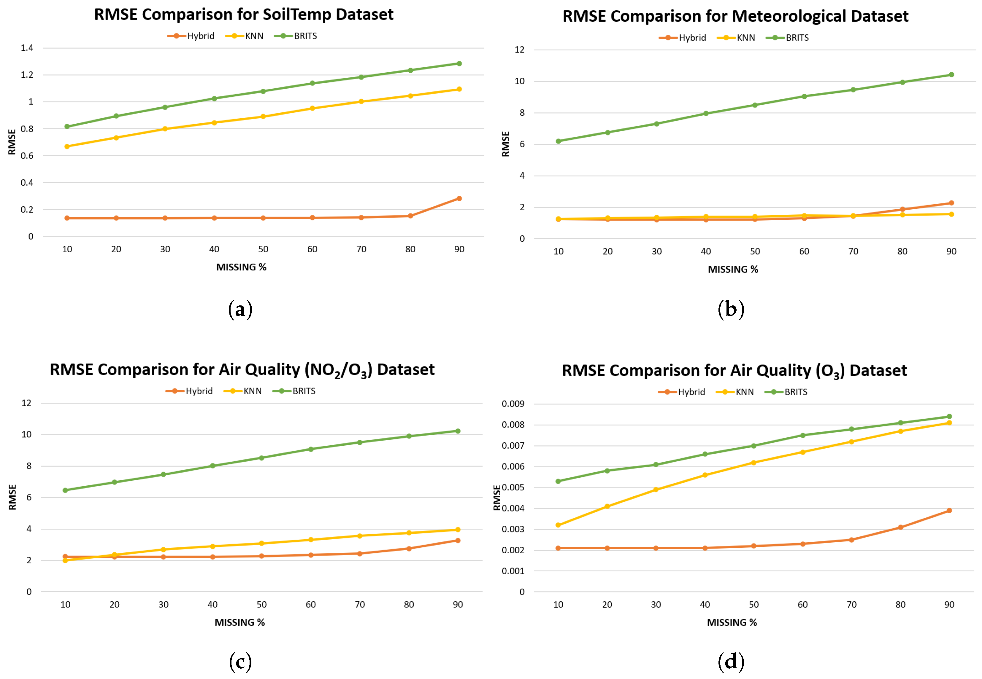
Figure 8.
Mean Absolute Error (MAE) comparison of different ablation variants for (a) SoilTemp, (b) Meteorological, (c) Air Quality NO2/O3, and (d) Air Quality O3 datasets.
Figure 8.
Mean Absolute Error (MAE) comparison of different ablation variants for (a) SoilTemp, (b) Meteorological, (c) Air Quality NO2/O3, and (d) Air Quality O3 datasets.
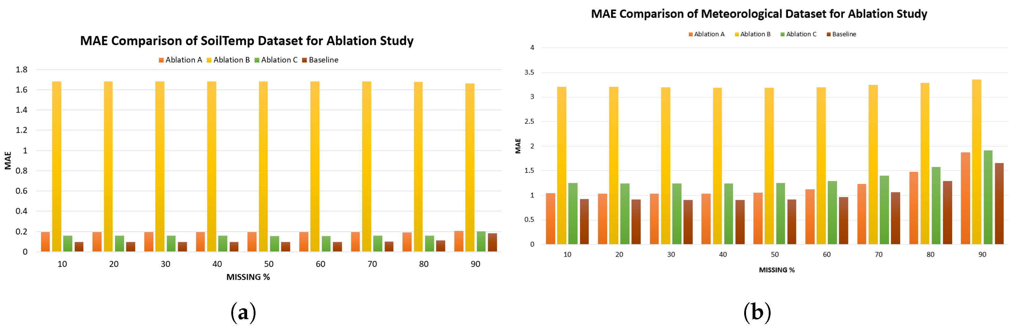
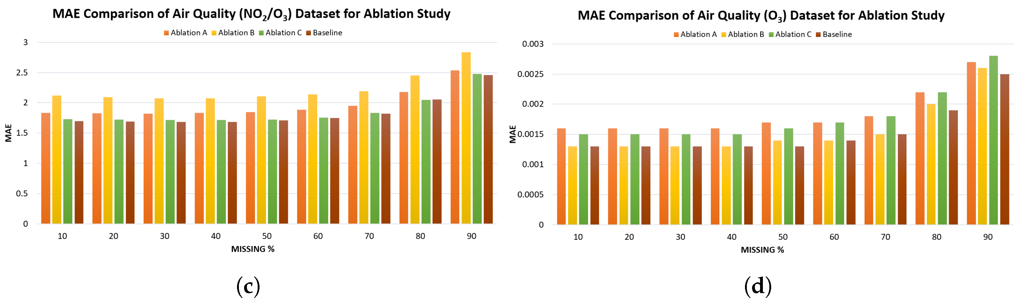
Figure 9.
Root Mean Squared Error (MAE) comparison of different ablation variants for (a) SoilTemp, (b) Meteorological, (c) Air Quality NO2/O3, and (d) Air Quality O3 datasets.
Figure 9.
Root Mean Squared Error (MAE) comparison of different ablation variants for (a) SoilTemp, (b) Meteorological, (c) Air Quality NO2/O3, and (d) Air Quality O3 datasets.
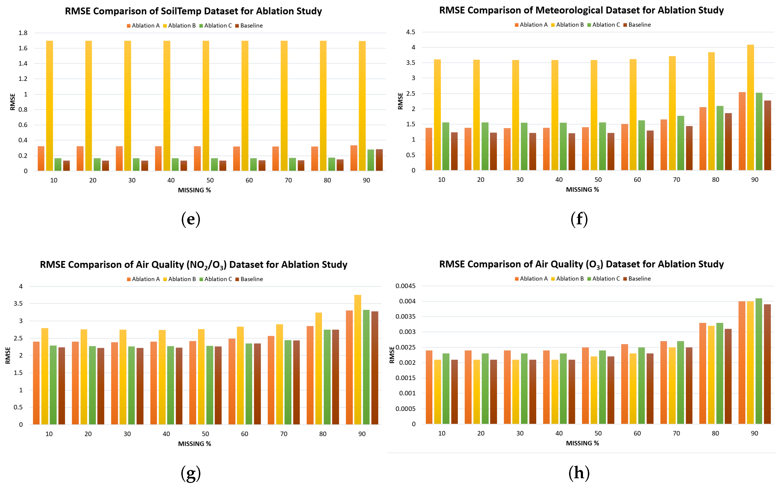
Figure 10.
Distribution comparison of target features in SoilTemp and Meteorological datasets.
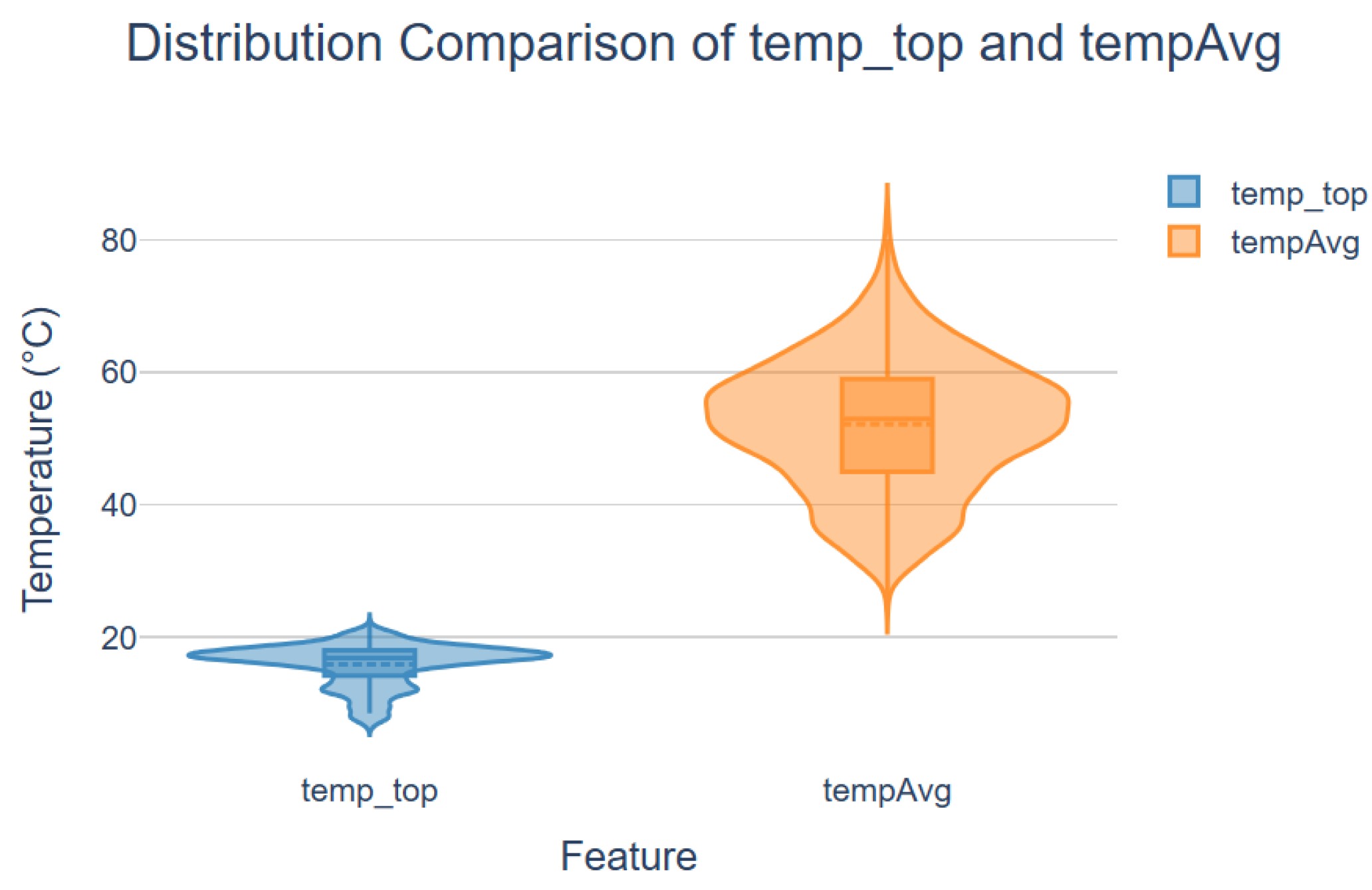

Table 1.
Model configuration and training parameters.
| Parameter | Value |
|---|---|
| 30 | |
| LSTM units | 64 |
| LSTM Activation function | ReLU |
| 0.3 | |
| Number of attention heads | 6 |
| 0.001 | |
| 32 | |
| 100 | |
| Loss function | Mean Squared Error (MSE) |
| Optimizer | Adam |
| Evaluation Metrics | RMSE, MAE |
Table 2.
Ablation study design and purpose.
| Model | LSTM1 | LSTM2 | Attention | Purpose |
|---|---|---|---|---|
| Baseline | ✓ | ✓ | ✓ | Full proposed hybrid model as baseline to compare |
| Ablation A | – | ✓ | ✓ | Test importance of pre-attention LSTM layer (LSTM1) |
| Ablation B | ✓ | – | ✓ | Test importance of post-attention LSTM layer (LSTM2) |
| Ablation C | ✓ | ✓ | – | Test contribution of attention and concatenation layers |
Table 3.
Performance of the model across varying missing rates for different environmental datasets.
Table 3.
Performance of the model across varying missing rates for different environmental datasets.
| Missing % | SoilTemp | Meteorological | Air Quality NO2/O3 | Air Quality O3 | |||||||
|---|---|---|---|---|---|---|---|---|---|---|---|
| MAE | RMSE | MAE | RMSE | MAE | RMSE | MAE | RMSE | ||||
| 10 | 0.0960 | 0.1366 | 0.9219 | 1.2350 | 1.6996 | 2.2337 | 0.0013 | 0.0021 | |||
| 20 | 0.0962 | 0.1369 | 0.9148 | 1.2264 | 1.6876 | 2.2233 | 0.0013 | 0.0021 | |||
| 30 | 0.0962 | 0.1368 | 0.9061 | 1.2159 | 1.6846 | 2.2214 | 0.0013 | 0.0021 | |||
| 40 | 0.0966 | 0.1370 | 0.9047 | 1.2091 | 1.6867 | 2.2317 | 0.0013 | 0.0021 | |||
| 50 | 0.0968 | 0.1374 | 0.9137 | 1.2219 | 1.7101 | 2.2627 | 0.0013 | 0.0022 | |||
| 60 | 0.0984 | 0.1387 | 0.9649 | 1.2992 | 1.7508 | 2.3456 | 0.0014 | 0.0023 | |||
| 70 | 0.1020 | 0.1417 | 1.0662 | 1.4390 | 1.8198 | 2.4350 | 0.0015 | 0.0025 | |||
| 80 | 0.1125 | 0.1525 | 1.2890 | 1.8602 | 2.0577 | 2.7507 | 0.0019 | 0.0031 | |||
| 90 | 0.1818 | 0.2839 | 1.6563 | 2.2737 | 2.4585 | 3.2772 | 0.0025 | 0.0039 | |||
Table 4.
MAE comparison of Hybrid, KNN, and BRITS imputation performance across varying missing rates for multiple environmental datasets.
Table 4.
MAE comparison of Hybrid, KNN, and BRITS imputation performance across varying missing rates for multiple environmental datasets.
| Missing % |
SoilTemp | Meteorological | Air Quality NO2O3 | Air Quality O3 | |||||||||||
|---|---|---|---|---|---|---|---|---|---|---|---|---|---|---|---|
| Hybrid | KNN | BRITS | Hybrid | KNN | BRITS | Hybrid | KNN | BRITS | Hybrid | KNN | BRITS | ||||
| 10 | 0.0960 | 0.2846 | 0.4136 | 0.9219 | 0.4915 | 3.0287 | 1.6996 | 0.8736 | 2.9713 | 0.0013 | 0.0012 | 0.0028 | |||
| 20 | 0.0962 | 0.3439 | 0.4963 | 0.9148 | 0.5537 | 3.6159 | 1.6876 | 1.1250 | 3.5071 | 0.0013 | 0.0018 | 0.0033 | |||
| 30 | 0.0962 | 0.4045 | 0.5733 | 0.9061 | 0.6051 | 4.2326 | 1.6846 | 1.3790 | 4.0402 | 0.0013 | 0.0024 | 0.0037 | |||
| 40 | 0.0966 | 0.4606 | 0.6561 | 0.9047 | 0.6744 | 4.9117 | 1.6867 | 1.6065 | 4.6357 | 0.0013 | 0.0030 | 0.0043 | |||
| 50 | 0.0968 | 0.5137 | 0.7269 | 0.9137 | 0.7324 | 5.5871 | 1.7101 | 1.8245 | 5.2438 | 0.0013 | 0.0036 | 0.0048 | |||
| 60 | 0.0984 | 0.5767 | 0.8080 | 0.9649 | 0.8205 | 6.2903 | 1.7508 | 2.0901 | 5.8750 | 0.0014 | 0.0042 | 0.0054 | |||
| 70 | 0.1020 | 0.6355 | 0.8800 | 1.0662 | 0.8679 | 6.9295 | 1.8198 | 2.3585 | 6.4875 | 0.0015 | 0.0049 | 0.0059 | |||
| 80 | 0.1125 | 0.6901 | 0.9573 | 1.2890 | 0.9477 | 7.6072 | 2.0577 | 2.5980 | 7.0493 | 0.0019 | 0.0054 | 0.0064 | |||
| 90 | 0.1818 | 0.7540 | 1.0380 | 1.6563 | 1.0320 | 8.2899 | 2.4585 | 2.8471 | 7.5503 | 0.0025 | 0.0060 | 0.0069 | |||
Table 5.
RMSE comparison of Hybrid, KNN, and BRITS imputation performance across varying missing rates for multiple environmental datasets.
Table 5.
RMSE comparison of Hybrid, KNN, and BRITS imputation performance across varying missing rates for multiple environmental datasets.
| Missing % |
SoilTemp | Meteorological | Air Quality NO2O3 | Air Quality O3 | |||||||||||
|---|---|---|---|---|---|---|---|---|---|---|---|---|---|---|---|
| Hybrid | KNN | BRITS | Hybrid | KNN | BRITS | Hybrid | KNN | BRITS | Hybrid | KNN | BRITS | ||||
| 10 | 0.1366 | 0.6698 | 0.8168 | 1.2350 | 1.2569 | 6.2026 | 2.2337 | 1.9988 | 6.4608 | 0.0021 | 0.0032 | 0.0053 | |||
| 20 | 0.1369 | 0.7338 | 0.8941 | 1.2264 | 1.3149 | 6.7579 | 2.2233 | 2.3625 | 6.9669 | 0.0021 | 0.0041 | 0.0058 | |||
| 30 | 0.1368 | 0.7996 | 0.9599 | 1.2159 | 1.3406 | 7.3109 | 2.2214 | 2.6911 | 7.4573 | 0.0021 | 0.0049 | 0.0061 | |||
| 40 | 0.1370 | 0.8460 | 1.0246 | 1.2091 | 1.4005 | 7.9559 | 2.2317 | 2.8881 | 8.0107 | 0.0021 | 0.0056 | 0.0066 | |||
| 50 | 0.1374 | 0.8919 | 1.0784 | 1.2219 | 1.3953 | 8.4931 | 2.2627 | 3.0765 | 8.5289 | 0.0022 | 0.0062 | 0.0070 | |||
| 60 | 0.1387 | 0.9520 | 1.1379 | 1.2992 | 1.4730 | 9.0417 | 2.3456 | 3.3174 | 9.0690 | 0.0023 | 0.0067 | 0.0075 | |||
| 70 | 0.1417 | 1.0026 | 1.1845 | 1.4390 | 1.4569 | 9.4659 | 2.4350 | 3.5606 | 9.5044 | 0.0025 | 0.0072 | 0.0078 | |||
| 80 | 0.1525 | 1.0453 | 1.2347 | 1.8602 | 1.5076 | 9.9458 | 2.7507 | 3.7530 | 9.8974 | 0.0031 | 0.0077 | 0.0081 | |||
| 90 | 0.2839 | 1.0947 | 1.2862 | 2.2737 | 1.5633 | 10.4219 | 3.2772 | 3.9535 | 10.2315 | 0.0039 | 0.0081 | 0.0084 | |||
Table 6.
MAE comparison across datasets for different ablation variants.
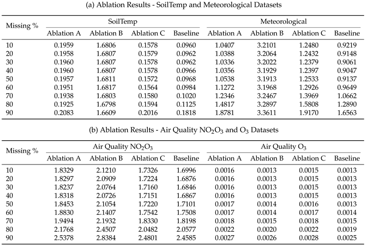 |
Table 7.
RMSE comparison across datasets for different ablation variants.
 |
Disclaimer/Publisher’s Note: The statements, opinions and data contained in all publications are solely those of the individual author(s) and contributor(s) and not of MDPI and/or the editor(s). MDPI and/or the editor(s) disclaim responsibility for any injury to people or property resulting from any ideas, methods, instructions or products referred to in the content. |
© 2025 by the authors. Licensee MDPI, Basel, Switzerland. This article is an open access article distributed under the terms and conditions of the Creative Commons Attribution (CC BY) license (http://creativecommons.org/licenses/by/4.0/).
Copyright: This open access article is published under a Creative Commons CC BY 4.0 license, which permit the free download, distribution, and reuse, provided that the author and preprint are cited in any reuse.


