

Submitted:
19 November 2025
Posted:
20 November 2025
You are already at the latest version
Abstract
A data-driven system identification algorithm which utilizes eigenvector is presented. The eigenvectors are extracted from an unified solution space comprising both input and output subspaces. To expand the input subspace, a higher-order subspace out of input subspaces are augmented with the measured input subspace; this higher-order subspace exhibit additional cross-correlations with both the input and output subspaces, thus producing more informative eigenvectors and linearizing the system. The extracted eigenvectors are then deployed to sequentially project new input snapshots first onto the input subspace and subsequently onto the output subspace to predict the output. The algorithm effectively reconstructs the original governing equations of a dynamic system, providing an inference that the original system is a series of data projection via eigenvectors, and also implying the possibility of reconstructing the low-rank governing equation with limited number of eigenvectors thus yielding a linearized representation of the system from the data. Notably, identifying the system from the well expanded, high-dimensional nonlinear solution space requires only a limited duration of data snapshots, indicating that the essential spatial features manifested by the governing equation are determined rapidly.
Keywords:
system identification
; eigenvector
; linear representation
Introduction
Multi-input multi-output models have been extensively employed as a form of multivariate regression and facilitated both academic and social advancements across diverse scientific domains, as prominently demonstrated by neural networks [1,2,3]. However, several inherent characteristics, e.g., the reliance on hyperparameter, the involvement of optimization, and overparameterized structures prone to overfitting, often confine models to likely serve as surrogates, limiting possible regression range near to the data space defined by the input feed. The fundamental objective of multivariate regression methods extends beyond constructing a surrogate: identifying the intrinsic features of the underlying system and enabling inference of a broad spectrum of potential system responses, i.e., data extrapolation, even from limited datasets [4]. From this perspective, while such surrogates may serve as effective intermediate regression modules, regression approaches that are grounded in linear transformations [5,6] and symbolic regression techniques [7,8,9,10] continue to receive significant attention, due to their capability to reveal interpretable and physically consistent system structures.
Multivariate Identification via Linear Projection of Eigenvectors (MILPE) algorithm presented in this study is also a linear transformation based regression technique that employs limited number of eigenvectors, typically equal to the dimension of input subspace, and is grounded in the principle that a given system can be fully or partially reconstructed through a linear combination of these eigenvectors, i.e., singular value decomposition (SVD) or principal component analysis [11], which has already shown the glimpse of possiblity of achieving linear representation of nonlinear system, as predicted by Koopman [12].
The direct utilization of eigenvectors for prediction has long been explored in approaches such as Galerkin projection [13], Gappy Proper Orthogonal Decomposition (Gappy-POD) [14,15], and Discrete Empirical Interpolation Method (DEIM) [16,17]. In most cases, eigenvectors have been extracted from systems defined within the state-variable space of the system itself, without explicitly incorporating input-output structure, and thus system reconstruction has typically relied on projection within this intrinsic space or on retaining the projection coefficients for reconstructing system behavior.
In line with these earlier frameworks, the MILPE algorithm also considers time invariant features; however, the eigenvectors are extracted within a space that jointly embeds both input and output subspaces. A higher rank, and thus a larger number of eigenvectors, is obtained by artificially augmenting this space with higher-order terms originating from the input subspace, facilitating the identification of an effective low-rank eigenvector set within the Hilbert space.
MILPE
Eigenvectors are derived as the left-eigenvector matrix obtained through eigenvalue decomposition of the cross-correlation matrix formed from the solution space , where rows correspond to variables and columns to data snapshots (Eq. 1). This left-eigenvector matrix defines an orthogonal coordinate system that is invariant to the ordering of snapshots and is oriented according to the statistical distribution among variables. Physically, the eigenvectors represent dominant patterns of mutual alignment among variables, functioning as principal axes of the convolution (i.e., cross-correlation or directional cosine) between data snapshots, indicating the degree to which variables evolve in similar directions across the ensemble of snapshots.
In order to function as a multi-input–multi-output model, MILPE extracts from a unified solution space in which arbitrary input subspaces and output subspaces are embedded together and are linearly independent, thus have non-zero cross-correlations:
The extracted represents the principal directions formed by the input data vectors () and output data vectors () used during training, yielding the truncated form when the trailing eigenvectors whose order exceeds the number of input variables are removed. The truncated matrix then naturally decomposes into as a pile of partial eigenvector sets associated with the input and output subspaces, denoted as and , respectively:
In prediction stage, the snapshot of input vector is firstly projected on and corresponding spans are estimated:
where the spans can be estimated with psuedoinverse of , i.e., .
The estimated are then used to span the for the prediction of output snapshot vector , under the assumption that the is a shared property between and . This assumption holds when and form orthogonal vector sets, similar to a full-projection case, where the remains identical across both subspaces:
Combining Eq. 5 and 6, the is expressed as follows:
Eq. (7) illustrates how an arbitrary input vector sequentially projects through the and components, obtained from the training data, to produce the output vector . The following sections present examples that have validated the current algorithm, along with additional interpretations derived from the results.
Lorenz System
Despite its structurally simple form, the Lorenz system [18] generates chaotic trajectories that diverge by small differences, reflecting its inherently nonlinear nature. Owing to this characteristics, the equations are employed as a canonical example in the validation of multivariate regression methods for the assessment of model accuracy [19].
In the current study, the system is simulated using a representative set of constant parameters and initial conditions that exhibit chaotic behavior [19]. After initializing the system, time integration is performed using the first-order Euler method with a time step seconds. The data obtained from the Lorenz system consist of trajectories (), higher-order terms fabricated with the trajectories () and corresponding velocity vectors (), which formed the input and output subspaces (i.e., and ), respectively, in the MILPE framework.
Figure 1 presents a comparison between the original simulation data and the MILPE prediction result. The data acquisition is acheived using the first seconds of simulation data corresponding to the time range where the governing equation begins to enter its asymptotic regime. Despite the limited training interval, the extracted eigenvectors clearly captures the cross-correlated structure between the input and output data, enabling an accurate trajectory prediction. Notably, the term effectively reconstructs the original governing equations (Figure 1, bottom right) that generated the original trajectory, even though the term is derived solely from data without prior knowledge of the Lorenz equations. An implication can be drawn that even in the absence of explicit governing equations, Eq. (7) potentially reconstruct the original equations as a sequential projection executed by partial eigenvectors obtained from the embedded input-output data space. In addition, since the term consists only of linear components, nonlinear systems may be effectively approximated as finite linear form having all the information in the limited eigenvectors. In this sense, the accuracy of extrapolation ultimately reflects the extent to which can be faithfully reconstructed from data, as governing equations inherently generate valid trajectories from arbitrary initial conditions.
The sources of error can be categorized into two primary factors: (1) the inclusion of input variables that do not directly influence the output variables during the eigenvector extraction process, e.g., the output variable is not correlated with or in the original governing equations, resulting in an incompletely linearized unified space and, consequently, less accurate eigenvectors; and (2) the truncation of the eigenvector set to match the number of input snapshots, which prevents the use of the remaining eigenvectors for projection. Both cases have been addressed and practically demonstrated in the subsequent examples.
Double-Pendulum
A fundamentally more stable form of the MILPE algorithm is presented for the double-pendulum problem, which features a substantially more complex governing equation of motion. This complexity necessitates deriving eigenvectors within a unified solution space that excludes input variables uncorrelated with the outputs, thereby isolating the input subspace corresponding to each individual output variable. The governing equations of the double pendulum are notably more intricate than those of the Lorenz system, as they involve second-order derivatives and trigonometric coupling terms.
The trajectory of the double pendulum is simulated using the equations of motion derived from Newton’s second law [20], with a time step s and first-order Euler time integration, consistent with the procedure adopted for the Lorenz system. The output variables are the angular accelerations, and the displacements are obtained by double time integration.
Figure 2 compares two distinct implementations: a global and a local approach. The global approach constructs the unified space directly from the original equations of motion assuming a optimum unified space and focuses on the quality of eigenvector projections derived from a limited data window. As shown in the prediction results, eigenvectors extracted from only 3s of data with the initial condition can accurately reconstruct the approximate governing equation and predict trajectories for a different initial condition, despite the latter being generally regarded as involving significantly stronger nonlinearity. The remaining challenge lies in formulating an optimum unified space without prior knowledge of the governing equations. Whereas the Lorenz system’s dominant structures are easily captured due to its simplicity, the double-pendulum system requires a specialized module or heuristic strategy to establish an appropriate unified space. The local approach demonstrates that a simplified unified space, constructed from a few truncated Taylor-series expansions of the dominant trigonometric terms, i.e., , , , , in systems with mild nonlinearity, can yield governing equation that achieve high accuracy within the vicinity of the training data. As predictions extend into regions of stronger nonlinear coupling, the accuracy of the reconstructed governing equations gradually deteriorates, indicating that while the eigenvectors are well resolved locally, higher-order and more sophisticated terms are required for global prediction. The local approach underscores the practicality of the MILPE framework for multivariate engineering problems exhibiting moderate nonlinearity, even in the absence of full governing equations, thereby enabling stable and efficient time marching.
Pressure Field on a Moving Cylinder Wall
As a third demonstration, a data set characterized by numerous noisy output variables correlated with only a few input variables is adopted. A methodology is proposed within the MILPE framework to incorporate more eigenvectors than the number of input variables, thereby addressing cases where the output dimensionality exceeds the input dimensionality. Although, in principle, one could formulate a separate governing equation for each output variable, as demonstrated in the second case, to achieve an exact representation of the unified space, the present approach prioritizes practicality and computational efficiency. It aims to leverage the MILPE algorithm to achieve an approximate full-projection in a unified manner.
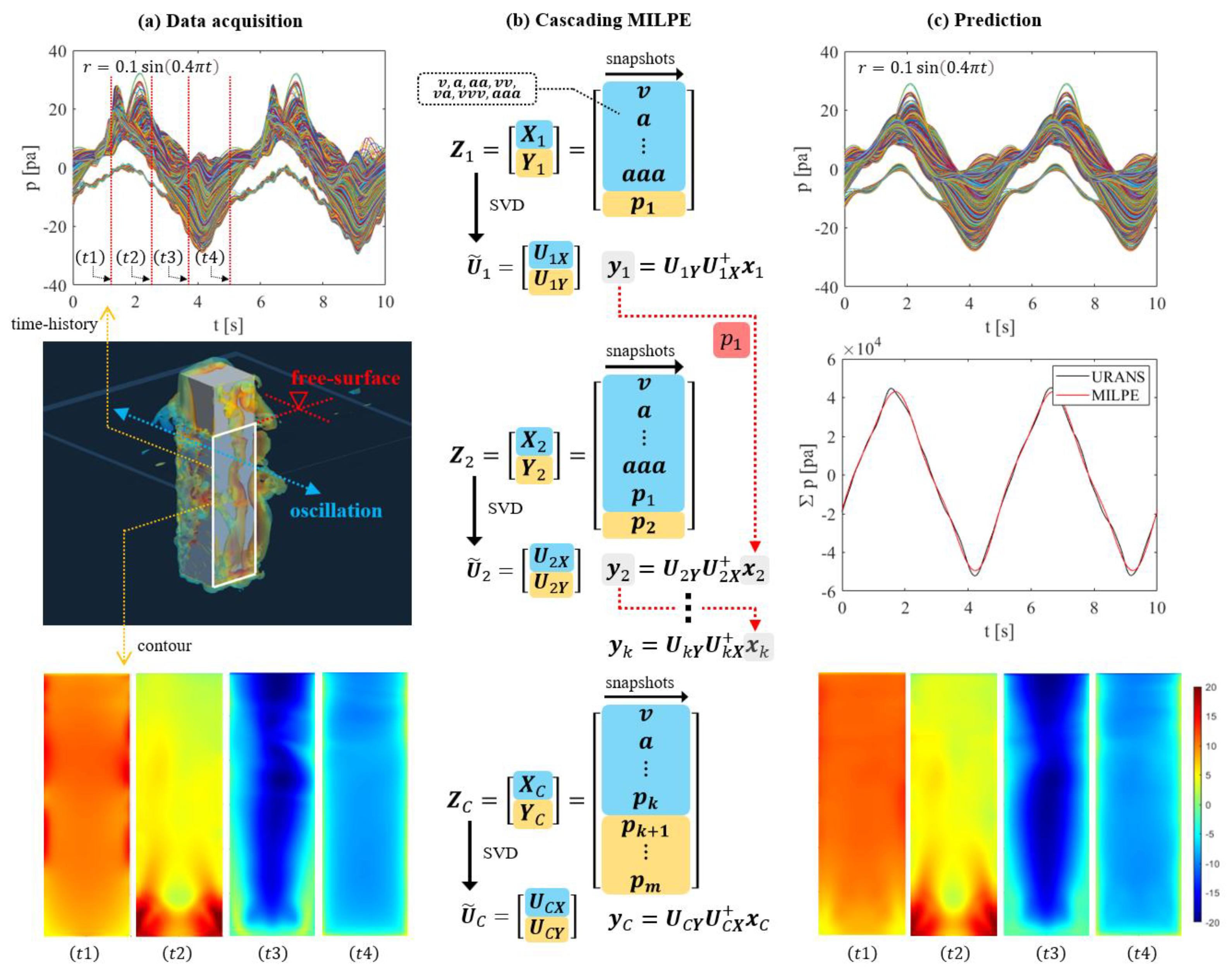
The data are obtained from incompressible unsteady Reynolds-Averaged Navier–Stokes (URANS) simulations of a forced-oscillating rectangular cylinder (Figure 3). Constructing a system based on this dataset aligns with long-standing efforts in reduced-order modeling (ROM) and their application to digital-twin technologies for estimating the service life of engineering systems [21,22,23,24]; comparable situations arise in many physics-based inference problems where limited control inputs drive high-dimensional responses. The cylinder is designed to oscillate while piercing the free-surface, allowing the load cell to measure the fluid-exerted forces without instrumental intereference from the experiment performed with the same condition, and these measurements are used to validate the simulations. For the MILPE application, 3072 piezometric pressure values are extracted from a cylinder wall facing the oscillation direction. These pressure signals exhibit dominant periods nearly identical to the oscillation period, but their degree of nonlinearity varies spatially along the wall due to difference in the onset of vortex shedding. Under the present conditions, approximately 99% of the total hydrodynamic force arise from pressure, with the remaining 1% attributed to frictional resistance. This dominance of pressure confirms the suitability of the current pressure data for modeling purposes.
A one degree of freedom sinosoidal forcing scenarios is simulated: , where denotes the cylinder displacement. The objective of the current ROM is to predict the pressure field as a function of kinematic variables that can, in principle, be obtained from sensor measurements. Accordingly, the pressure data are treated as outputs, while the measurable kinematic quantities, velocity and acceleration , serve as inputs. Although the displacement could be used in place of since it is prescribed as a sine function, acceleration is preferred as it aligns naturally with the conventional added-mass concept. Strictly speaking, there is no definitive rule dictating that pressure must be an explicit function of these kinematic variables. Rather, the present demonstration assumes that pressure is closely correlated with the kinematic environment, as the controlled variable in this setup is motion alone.
As in the previous demonstrations, Figure 3 illustrates the training data, the MILPE process, and the corresponding prediction results. As mentioned earlier, the present condition involves a limited number of input measurements, velocity and acceleration, and their higher-order combinations (, , , , ) that must be used to regress a large number of output variables. The input subspace is seven-dimensional, and representing more than 3000 pressure outputs with only seven eigenvectors is both intuitively and inherently challenging. Therefore, a hybrid approach combining the previous methods, referred to as cascading MILPE, is applied. Among the 3072 pressure data points, the one showing the highest linear correlation with the current input subspace is first identified and computed through a single MILPE; the resulting pressure is then reintroduced as an additional input to form the next input subspace. This cascading process continued up to the th step, resulting in an initial input subspace augmented with 30 pressure variables and thus employing 30 eigenvectors in total.
Inspection of the predicted time series shows that most dominant features are well resolved. The integrated pressure, corresponding to the force (since the pressure grids were designed to be uniformly distributed over an equal surface area), closely follows the original URANS results even under strongly nonlinear conditions. The most notable deviation occurs around 1.25 s (marked as in Figure 3a), where the first sharp spike within the cycle is not captured. This event is of particular interest since it could represent a transient stress peak on the structure. Two potential causes are identified: (1) the corresponding pressure data exhibit weak correlation with the initial input subspace; and (2) the system has not yet reached a near full-projection condition. However, since the solution converged to the same value even as increased, the first cause appears dominant.
Considering that the governing equation reconstructed by MILPE originates from the covariance matrix, the result implies a lack of input subspace components strongly correlated with that signal. From the signal characteristics, it is expected that an input subspace with higher frequency content would improve correlation. In the present setup, the highest frequency terms, such as or , oscillate only three times faster than the base signals. Adding higher-frequency subspace components, however, may introduce difficulty in distinguishing signal from noise or lead to their inclusion among eigenvectors deemed insignificant due to their smaller variance. Moreover, since correlation is affected not only by frequency but also by phase difference, further separation of signals by phase is expected to enhance prediction accuracy. While noise was not treated explicitly, the least-squares based construction of eigenvectors inherently accounts for it to some degree, ensuring adequate accuracy. Additional tests, conducted using the derived governing equation under a different forced-motion scenario, , confirmed that the reconstructed equation successfully captured dominant local trends similar to those observed in the previous two demonstrations though the degree of difference in nonlinearity remains to be evaluated.
Discussion
Three types of regression techniques within the structure of the MILPE algorithm are presented to demonstrate: (1) the basic emergence of governing equations from eigenvectors; (2) the level of complexity that MILPE can handle under ideal conditions and its capability to reconstruct local governing equations for practical applications; and (3) an alternative approach that utilizes a greater number of eigenvectors. The algorithm is believed to offer a new perspective on establishing data-driven multi-input–multi-output regression models. Its advantage lies in being mathematically well-defined and fully traceable.
The governing equation constructed from the current algorithm is determined at the stage of constructing the covariance matrix, implying that the obtainable governing equations are inherently defined by the correlations within the data. To construct a completely linearized unified space using the arbitrary data, a deeper understanding of these correlations may be required. As of now, no module exists that can perfectly generate such a unified space. If developing one proves too complex, constructing multiple governing equations for different data ranges and interpolating between them, a surrogate modeling approach, could be a practical alternative.
In all demonstrations, the raw input and output subspaces were not manipulated, whether by mean subtraction or normalization. Such preprocessing might alter the order or magnitude of the principal eigenvectors used for projection during prediction, which warrants further investigation. If appropriate manipulation by itself can render the system more linear, the number of required input subspace dimensions could be substantially reduced. However, since the system must be de-manipulated once the outputs are obtained, an additional step is necessary to interpret the differences between the manipulated and the original systems. Although not equivalent to system manipulation, localizing the grid in the URANS solution could similarly linearize the signal when constructing a ROM, as much of the response would then depend linearly on the kinematics. For simple systems such as the Lorenz case, normalization of subspaces yielded governing equations identical to those derived from the raw subspaces.
Finally, the number of projected eigenvectors exactly matched the number of input variables in all demonstrations; however, in noisy datasets where unwanted eigenvectors may appear due to noise contamination, reducing the projection dimension by excluding such eigenvectors could also be considered.
Acknowledgments
The author gratefully acknowledges Dr. Myoung-soo Kim of the Korea Research Institute of Ships and Ocean Engineering (KRISO) for proposing a fundamental experiment and sharing the experimental data.
References
- Vaswani, A., Shazeer, N., Parmar, N., Uszkoreit, J., Jones, L., Gomez, A.N., Kaiser, Ł. and Polosukhin, I., 2017. Attention is all you need. Advances in neural information processing systems, 30.
- Krizhevsky, A., Sutskever, I. and Hinton, G.E., 2012. Imagenet classification with deep convolutional neural networks. Advances in neural information processing systems, 25.
- Eivazi, H., Tahani, M., Schlatter, P. and Vinuesa, R., 2022. Physics-informed neural networks for solving Reynolds-averaged Navier–Stokes equations. Physics of Fluids, 34(7).
- Brunton, S.L. and Kutz, J.N., 2022. Data-driven science and engineering: Machine learning, dynamical systems, and control. Cambridge University Press.
- Schmid, P.J., 2010. Dynamic mode decomposition of numerical and experimental data. Journal of fluid mechanics, 656, pp.5-28. [CrossRef]
- Brunton, S.L., Proctor, J.L., Tu, J.H. and Kutz, J.N., 2015. Compressed sensing and dynamic mode decomposition. Journal of computational dynamics, 2(2). [CrossRef]
- Brunton, S.L., Proctor, J.L. and Kutz, J.N., 2016. Discovering governing equations from data by sparse identification of nonlinear dynamical systems. Proceedings of the national academy of sciences, 113(15), pp.3932-3937. [CrossRef]
- Champion, K., Lusch, B., Kutz, J.N. and Brunton, S.L., 2019. Data-driven discovery of coordinates and governing equations. Proceedings of the National Academy of Sciences, 116(45), pp.22445-22451. [CrossRef]
- Rudy, S.H., Brunton, S.L., Proctor, J.L. and Kutz, J.N., 2017. Data-driven discovery of partial differential equations. Science advances, 3(4), p.e1602614. [CrossRef]
- Brunton, S.L., Zolman, N., Kutz, J.N. and Fasel, U., 2025. Machine learning for sparse nonlinear modeling and control. Annual Review of Control, Robotics, and Autonomous Systems, 8. [CrossRef]
- Eckart, C. and Young, G., 1936. The approximation of one matrix by another of lower rank. Psychometrika, 1(3), pp.211-218. [CrossRef]
- Koopman, B.O., 1931. Hamiltonian systems and transformation in Hilbert space. Proceedings of the National Academy of Sciences, 17(5), pp.315-318. [CrossRef]
- Sirovich, L., 1987. Turbulence and the dynamics of coherent structures. I. Coherent structures. Quarterly of applied mathematics, 45(3), pp.561-571. [CrossRef]
- Everson, R. and Sirovich, L., 1995. Karhunen–Loeve procedure for gappy data. Journal of the Optical Society of America A, 12(8), pp.1657-1664.
- Willcox, K., 2006. Unsteady flow sensing and estimation via the gappy proper orthogonal decomposition. Computers & fluids, 35(2), pp.208-226. [CrossRef]
- Chaturantabut, S. and Sorensen, D.C., 2010. Nonlinear model reduction via discrete empirical interpolation. SIAM Journal on Scientific Computing, 32(5), pp.2737-2764. [CrossRef]
- Peherstorfer, B., Butnaru, D., Willcox, K. and Bungartz, H.J., 2014. Localized discrete empirical interpolation method. SIAM Journal on Scientific Computing, 36(1), pp.A168-A192. [CrossRef]
- Lorenz, E.N., 2017. Deterministic nonperiodic flow 1. In Universality in Chaos, 2nd edition (pp. 367-378). Routledge.
- Brunton, S.L., Zolman, N., Kutz, J.N. and Fasel, U., 2025. Machine learning for sparse nonlinear modeling and control. Annual Review of Control, Robotics, and Autonomous Systems, 8. [CrossRef]
- Shinbrot, T., Grebogi, C., Wisdom, J. and Yorke, J.A., 1992. Chaos in a double pendulum. American Journal of Physics, 60(6), pp.491-499. [CrossRef]
- Kapteyn, M.G. and Willcox, K.E., 2022. Design of digital twin sensing strategies via predictive modeling and interpretable machine learning. Journal of Mechanical Design, 144(9), p.091710. [CrossRef]
- Niederer, S.A., Sacks, M.S., Girolami, M. and Willcox, K., 2021. Scaling digital twins from the artisanal to the industrial. Nature Computational Science, 1(5), pp.313-320. [CrossRef]
- Kapteyn, M.G., Knezevic, D.J., Huynh, D.B.P., Tran, M. and Willcox, K.E., 2022. Data-driven physics-based digital twins via a library of component-based reduced-order models. International Journal for Numerical Methods in Engineering, 123(13), pp.2986-3003.
- Benner, P., Gugercin, S. and Willcox, K., 2015. A survey of projection-based model reduction methods for parametric dynamical systems. SIAM review, 57(4), pp.483-531. [CrossRef]
Figure 1.
Demonstration of MILPE application to the Lorenz system: (a) governing equation of the original Lorenz system and the achieved trajectories with the initial condition . The trajectory for the first seconds (symbol) is used for the extraction of eigenvectors. (b) the augmented data space for the extraction of eigenvectors (), truncated eigenvectors () and the partial eigenvectors (,). (c) reconstructed governing equation () and the comparison between the predicted and the original trajectories.
Figure 1.
Demonstration of MILPE application to the Lorenz system: (a) governing equation of the original Lorenz system and the achieved trajectories with the initial condition . The trajectory for the first seconds (symbol) is used for the extraction of eigenvectors. (b) the augmented data space for the extraction of eigenvectors (), truncated eigenvectors () and the partial eigenvectors (,). (c) reconstructed governing equation () and the comparison between the predicted and the original trajectories.
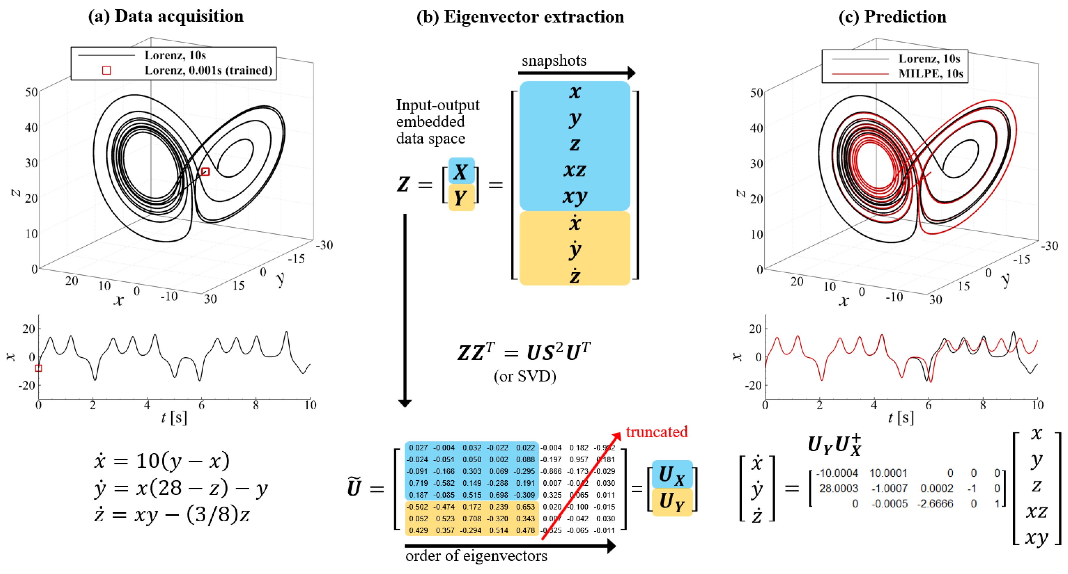
Figure 2.
Demonstration of MILPE application to the Double-pendulum (DP) problem: (a) equation of motion, geometrical and physical properties of the double-pendulum system and the achieved trajectories with the initial condition . The trajectory for the first 3 seconds (red line) is used for the extraction of eigenvectors. (b) extraction of the eigenvectors using global (b.1) and local (b.2) augmented input subspaces (c) reconstructed governing equations and the comparison between the predicted and the original trajectories.
Figure 2.
Demonstration of MILPE application to the Double-pendulum (DP) problem: (a) equation of motion, geometrical and physical properties of the double-pendulum system and the achieved trajectories with the initial condition . The trajectory for the first 3 seconds (red line) is used for the extraction of eigenvectors. (b) extraction of the eigenvectors using global (b.1) and local (b.2) augmented input subspaces (c) reconstructed governing equations and the comparison between the predicted and the original trajectories.
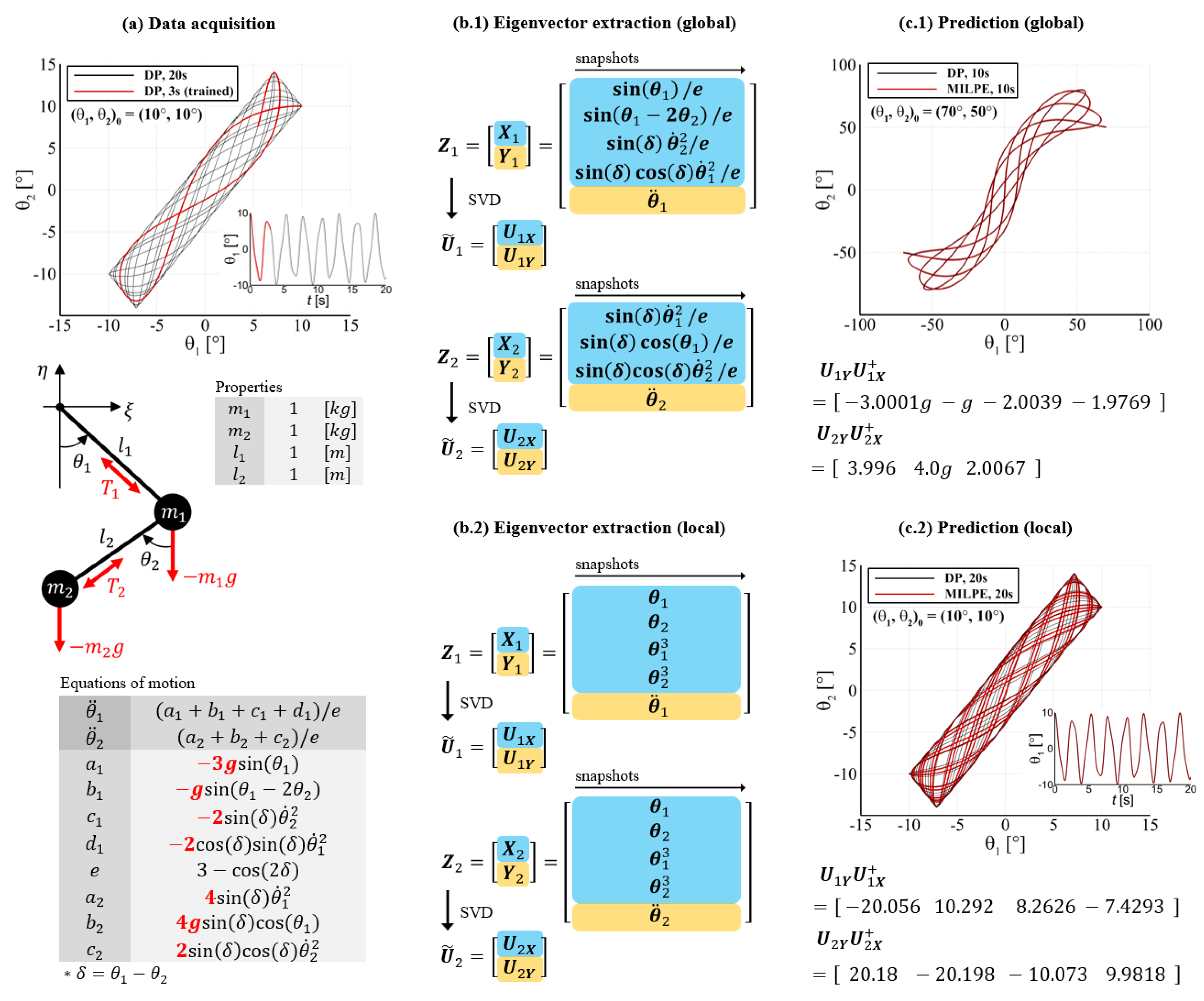
Figure 3.
Demonstration of MILPE application to the CFD pressure field of a moving rectangular cylinder: (a) Schematic of the problem setup, showing the oscillating cylinder, free surface, and time histories of the pressure field on a selected wall (white rectangle), along with pressure contours at t1-4. (b) The first two consecutive steps in the cascading MILPE procedure and the resulting configuration of the reconstructed governing equation. (c) Predicted time histories of the wall pressure and the integrated pressure compared with URANS results, together with corresponding pressure contours at t1-4.
Figure 3.
Demonstration of MILPE application to the CFD pressure field of a moving rectangular cylinder: (a) Schematic of the problem setup, showing the oscillating cylinder, free surface, and time histories of the pressure field on a selected wall (white rectangle), along with pressure contours at t1-4. (b) The first two consecutive steps in the cascading MILPE procedure and the resulting configuration of the reconstructed governing equation. (c) Predicted time histories of the wall pressure and the integrated pressure compared with URANS results, together with corresponding pressure contours at t1-4.
Disclaimer/Publisher’s Note: The statements, opinions and data contained in all publications are solely those of the individual author(s) and contributor(s) and not of MDPI and/or the editor(s). MDPI and/or the editor(s) disclaim responsibility for any injury to people or property resulting from any ideas, methods, instructions or products referred to in the content. |
© 2025 by the authors. Licensee MDPI, Basel, Switzerland. This article is an open access article distributed under the terms and conditions of the Creative Commons Attribution (CC BY) license (http://creativecommons.org/licenses/by/4.0/).
Copyright: This open access article is published under a Creative Commons CC BY 4.0 license, which permit the free download, distribution, and reuse, provided that the author and preprint are cited in any reuse.