SEQUENTION: A Timeless Biological Framework for Foliated Change and 4D-Counterduction

1. Introduction

Biology is saturated with temporal language. Organisms develop, populations adapt, lineages diverge, traits recur, environments change, and histories accumulate. This vocabulary is empirically indispensable. Population genetics, phylogenetics, paleontology, developmental biology, ecology, and experimental evolution all depend on ordered records and time-indexed models. SEQUENTION does not discard those disciplines or deny their shadow-level explanatory power. It asks a different foundational question: whether elapsed time is the ontic producer of biological form, or whether the observed sequence is the operational presentation of source-level constraints through a three-dimensional biological shadow [1,2].

The distinction matters because several recurrent features of biological organization resist treatment as unconstrained temporal search. Development is canalized; morphospace is highly restricted; independent lineages converge; modular systems can recover stable endpoints after perturbation; and function can persist despite substantial genomic rearrangement. Standard biology already explains many of these facts through selection, developmental architecture, physical constraint, pleiotropy, network structure, and ecology. SEQUENTION retains those mechanisms as effective descriptions. Its additional claim is ontological: the stability that those mechanisms reveal may be the shadow-readable expression of a complete source architecture rather than a product assembled by time itself.

Earlier formulations described the living biosphere as a three-dimensional shadow of a four-dimensional Counterspace and called its ordered presentation a foliation. That language was easily confused with two established images. First, “four-dimensional” was read as three spatial axes plus time. Second, “projection” was read as holography. Both readings are incorrect. The four dimensions belong to a non-temporal Counterspace source. The biological shadow is not a constant-time slice of a spacetime manifold, and it is not necessarily a boundary encoding from which the source can be reconstructed. The present paper therefore incorporates the foundational term 4D-Counterduction: the ECL-governed constitutive realization by which complete four-dimensional source content becomes a selector-indexed biological readout. This term is not a replacement name for Counterspace. Counterspace names the complete source domain; biological Counterduction names the relation by which that source becomes readable in the biological Shadow.

The second major refinement concerns the Extrinsic Constitutive Law (ECL). The ECL is not a scalar biological force, not an invariant, not a vital substance, and not a mind-like agent. It is the source-grounded readability law whose domain reductions make biological invariants and artifacts operationally distinguishable [3,4]. The latest type discipline separates the law, its complete profile, and one selected readout. This prevents the biological potential U, mobility ${\mu }_{\mathrm{bio}}$, or embedding scale $a^{†}$ from being elevated into independent source primitives.

The third refinement is methodological. A timeless source ontology does not immunize biological maps from failure. A candidate convergence curvature can fail to recur. A proposed endpoint invariant can dissolve under a better morphospace embedding. A biological scale can fail to transfer across taxa. A non-local kernel can prove unnecessary because a local model explains the same data. Such failures refute the corresponding maps and force revision. The scientific programme is cartographic because it seeks source-conditioned invariants through partial readouts; it is accountable because every map must carry a failure condition [2,5].

This paper pursues seven objectives. It defines biological 4D-Counterduction; restates the four framework axioms in biological form; types the source, ECL profile, selector, and readout; formalizes scalar and tensorial biological reductions; distinguishes invariants from artifacts, assumptions, and interpretations; develops nine operational candidate invariants and associated experimental protocols; and audits the roles of geochemical source tracing, multifractality, nonlinear dynamics, collective behaviour, probability, and finite-resource abiogenesis. The result is a standalone biological foundation rather than an appendix to the gravitational sector.

2. 4D-Counterduction in the Biological Sector

2.1. Definition

Definition 1

(Biological 4D-Counterduction). Biological 4D-Counterduction is the selector-indexed, ECL-governed realization by which the informational organization of a complete four-dimensional Counterspace configuration becomes operationally readable as genotype–phenotype–environment structure, developmental ordering, ecological relation, and biological history in a three-dimensional shadow, with the ordering label defined only up to admissible gauge reparameterization and biological clock time constructed within the shadow rather than installed as a source dimension.

2.1.0.1. Biological non-substitution principle.

Biological 4D-Counterduction does not replace, rename, or supersede four-dimensional Counterspace. Counterspace is the complete non-temporal source ontology shared by the framework. Biological Counterduction is the domain-specific, ECL-governed relation by which that source is registered as a biological Shadow. It presupposes Counterspace and has no independent source content, source geometry, or ontological dimensionality. The qualifier “4D” identifies the source of the realization, not Counterduction as a second four-dimensional object. Thus,

$$\begin{array}{|c|}\hline \begin{array}{cc}\hfill 4\mathrm{D}\mathrm{Counterspace}& \neg \equiv \mathrm{biological}4\mathrm{D}-\mathrm{Counterduction},\hfill \\ \hfill \mathrm{source}\mathrm{ontology}& \neg \equiv \mathrm{biological}\mathrm{source}-\mathrm{to}-\mathrm{shadow}\mathrm{relation}.\hfill \end{array}\\ \hline\end{array}$$

(1)

The compact expression is

$${\mathcal{C}}^4\stackrel{{Ctd}_{4,\mathrm{bio}}^{\sigma }}{\to }{\Sigma }_{\mathrm{bio}}^3[{\lambda }_g;{\tau }_{\mathrm{bio}}],{\lambda }_g\sim h\left({\lambda }_g\right),{\tau }_{\mathrm{bio}}=\mathrm{operational}\mathrm{biological}\mathrm{clock}.$$

(2)

The arrow denotes constitutive realization, not temporal development of the source. A developmental trajectory, fossil sequence, or laboratory time series is a shadow record ordered by ${\lambda }_g$; it is not a motion of the complete source through a temporal dimension.

The non-slice condition is

$$\begin{array}{|c|}\hline {\Sigma }_{\mathrm{bio}}^3[{\mathcal{F}}_{\mathrm{bio}},{\lambda }_g;{\tau }_{\mathrm{bio}}]\ne {\left.{\mathcal{C}}^4\right|}_{t={\tau }_{\mathrm{bio}}}.\\ \hline\end{array}$$

(3)

Thus a biological “stage” is not an ontic constant-time section of Counterspace. It is one admissible biological readout of complete source content.

2.2. Typed Source-to-Readout Chain

Let $\Xi \in {\mathfrak{X}}_{\mathrm{adm}}$ be a complete admissible source configuration and define

$$Info:{\mathfrak{X}}_{\mathrm{adm}}\to {\mathfrak{I}}_{\mathrm{src}},{\mathfrak{M}}_{\Xi }=Info\left(\Xi \right).$$

(4)

The symbol ${\mathfrak{M}}_{\Xi }$ denotes non-experiential source information. It is not individual consciousness, intention, or agency. Let

$${\sigma }_{\mathrm{bio}}=(X_{\mathrm{bio}},\left[s\right],B_{\mathrm{bio}},P_{\mathrm{bio}})$$

(5)

be a biological selector containing the immersion, foliation class, biological corridor or boundary data, and a domain projector. These objects select a biological reading; they do not contribute additional source content.

If $Y_{\sigma }$ is the biological readout space, define

$${\mathfrak{P}}_{\mathrm{read}}=\prod _{\sigma \in {\mathfrak{S}}_{\mathrm{adm}}}{Y}_{\sigma },{Read}_{S,G}:{\mathfrak{I}}_{\mathrm{src}}\to {\mathfrak{P}}_{\mathrm{read}},$$

(6)

and

$$\begin{array}{cc}\hfill {\mathcal{E}}_S& ={Read}_{S,G}\circ Info:{\mathfrak{X}}_{\mathrm{adm}}\to {\mathfrak{P}}_{\mathrm{read}},\hfill \end{array}$$

(7)

$$\begin{array}{cc}\hfill {\mathcal{E}}_{S,\Xi }& ={\mathcal{E}}_S\left(\Xi \right),\hfill \end{array}$$

(8)

$$\begin{array}{cc}\hfill {\mathcal{E}}_{S,\Xi }^{\sigma }& ={ev}_{{\sigma }_{\mathrm{bio}}}\left({\mathcal{E}}_{S,\Xi }\right).\hfill \end{array}$$

(9)

A physical or biological observability map ${\pi }_{\sigma }^{\mathrm{bio}}$ can then produce the registered quantities used by experiments. The counterduction map is

$${Ctd}_{4,\mathrm{bio}}^{\sigma }={\pi }_{\sigma }^{\mathrm{bio}}\circ {ev}_{\sigma }\circ {Read}_{S,G}\circ Info.$$

(10)

Equation (10) is a typed composition acting on an admissible source configuration; it is therefore categorically distinct from the Counterspace source domain that it presupposes.

Figure 1. Biological 4D-Counterduction. Counterspace remains the antecedent source ontology; biological Counterduction is the source-to-readout relation. The biological selector evaluates one source-grounded profile into an operational state-space representation. The sequence is logical rather than temporal.

Figure 1. Biological 4D-Counterduction. Counterspace remains the antecedent source ontology; biological Counterduction is the source-to-readout relation. The biological selector evaluates one source-grounded profile into an operational state-space representation. The sequence is logical rather than temporal.

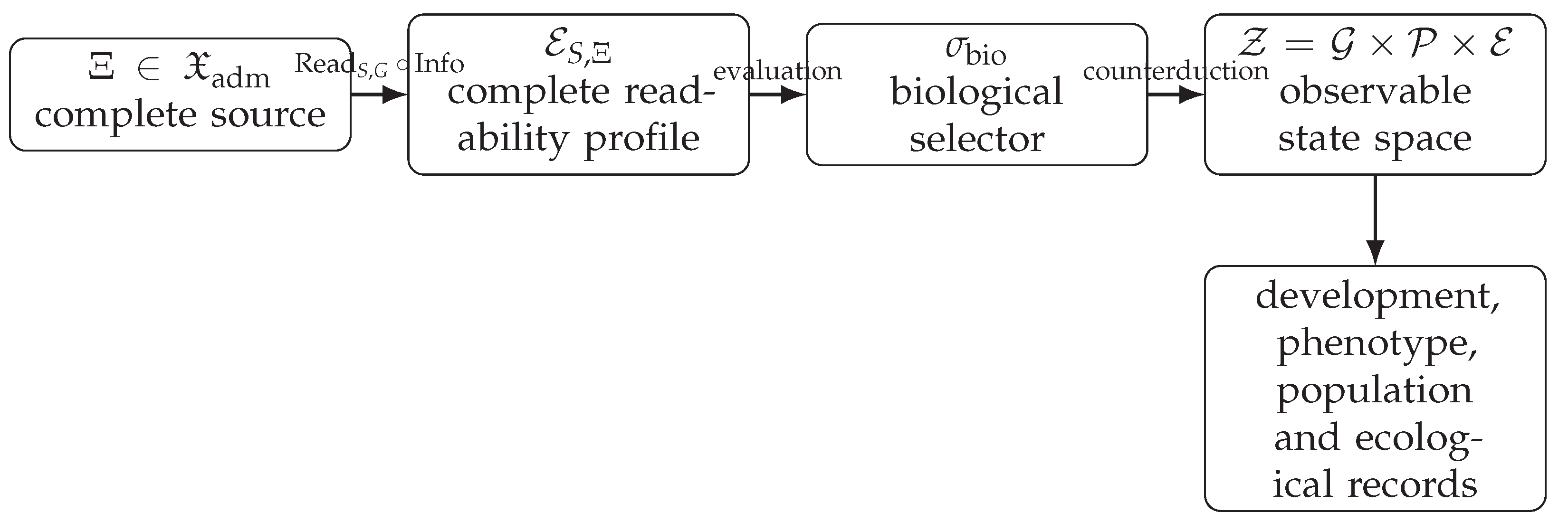
The stronger notation ${\mathfrak{M}}_{\Xi }={\mathcal{E}}_{S,\Xi }$ is not used as literal equality because the objects occupy different formal spaces. One may retain only a conditional ontic co-reference,

$${\mathfrak{M}}_{\Xi }{\equiv }_{\mathrm{ont}}{\mathcal{E}}_{S,\Xi },$$

(11)

if all source information is exhausted by the complete family of admissible readouts. The Epistemic Cut leaves that exhaustion condition open [4,6].

2.3. Why Counterduction Is Preferable to Holography in Biology

The biological source–shadow relation differs from simple holography in four ways. The biosphere need not be a geometric boundary of Counterspace. Biological readouts need not contain a globally invertible encoding. The fourth source dimension is not time. Finally, the biological shadow is not an illusion: organisms, environments, developmental interactions, and histories are physically real within the readout domain even though they do not exhaust the source.

A many-to-one relation is expected. Distinct source distinctions can be observationally equivalent under one biological selector while separating under another. A gene sequence, for example, can vary while preserving a functional corridor; a phenotype can recur through different developmental routes; and one morphometric chart can erase distinctions visible in another. The framework therefore locates biological invariance in selector-stable organization rather than automatically in one molecular token [7].

2.4. The Biological Minkowski Trap: Chronology Is Not Source Dimensionality

The biological form of the Minkowski trap is not the use of chronological variables. Developmental age, generation number, divergence time, stratigraphic position, physiological duration, and laboratory sampling time are indispensable coordinates of biological evidence. The trap occurs only when the success of those coordinates is promoted into the ontological claim that time is a dimension of the complete biological source, or when elapsed duration is treated as a causally sufficient substance rather than as an ordering variable within a specified biological model [8].

The corresponding non-entailment is

$$\begin{array}{|c|}\hline \underset{\mathrm{shadow}-\mathrm{level}\mathrm{coordinate}\mathrm{statement}}{\underbrace{t,n,{\tau }_{\mathrm{dev}},{\tau }_{\mathrm{strat}}\mathrm{organize}\mathrm{biological}\mathrm{records}}}\nRightarrow \underset{\mathrm{source}-\mathrm{ontological}\mathrm{statement}}{\underbrace{t\in Dim\left({\mathcal{C}}^4\right)}}.\\ \hline\end{array}$$

(12)

SEQUENTION therefore does not discard historical biology. It keeps phylogenetic order, fossil succession, rates, generation intervals, population histories, and developmental timing as operationally real features of the biological shadow. It denies that their temporal coordinate is the fourth dimension of Counterspace.

The same three-way distinction used in the physical foundation must be retained biologically. Let

$${\mathcal{F}}_{\mathrm{bio}}={\left\{X_{\lambda }^{\mathrm{bio}}:{\Sigma }_{\mathrm{bio}}\hookrightarrow \mathcal{C}\right\}}_{\lambda \in I}$$

(13)

be an admissible family of biological readouts. The family has geometric and biological content because it constrains which genotype–phenotype–environment registrations are jointly admissible. Its bare label is gauge, $\lambda \sim h\left(\lambda \right)$. Operational biological time is instead constructed from biological clocks and records,

$${\tau }_{\mathrm{bio}}={\mathcal{T}}_{\mathrm{bio}}\left[\mathrm{developmental}\mathrm{markers},\mathrm{generation}\mathrm{counts},\mathrm{physiological}\mathrm{clocks},\mathrm{stratigraphic}\mathrm{records}\right].$$

(14)

Consequently,

$$\begin{array}{|c|}\hline {\mathcal{F}}_{\mathrm{bio}}\neg \equiv {\lambda }_g\neg \equiv {\tau }_{\mathrm{bio}},t_{\mathrm{ont}}\notin Dim\left({\mathcal{C}}^4\right).\\ \hline\end{array}$$

(15)

This distinction blocks two opposite errors. One error is to convert chronological description into a temporal source ontology. The other is to infer that because time is non-ontic, chronological evidence can be ignored. SEQUENTION permits neither move. A biological history remains an empirical record that any admissible map must recover. 4D-Counterduction changes the level at which that history is interpreted: the ordered record is a counterduced shadow expression of complete source organization, not a sequence generated by motion of the source through a temporal axis.

3. Axioms of SEQUENTION in Biology

3.1. A1: Whole Biological Content

A1. There exists a complete four-dimensional Counterspace $(\mathcal{C},G,\Psi )$ whose admissible biological readouts include the full content of viable genotype–phenotype–environment relations. The biological shadow does not add source content; it registers a domain-specific projection.

A1 does not assert that every logically imaginable organism exists in one shadow. It states that the source contains the content relevant to the complete family of admissible biological readouts. The admissibility structure is constrained, and the absence of observed forms can reflect source-conditioned boundaries rather than merely incomplete temporal search.

3.2. A2: Identity of Source and Singular Biological Organization

A2. A distinguished source origin $p_0$ generates a conserved singular set

$$S=Orb\left(p_0\right).$$

(16)

Stable developmental organizers, recurrent corridor boundaries, and repeated structural solutions can be investigated as shadow expressions of this singular architecture.

This axiom must not be translated into a hidden developmental particle or a local mystical attractor. The singular set is a source-level identity relation. Ordinary developmental mechanisms remain indispensable at the shadow level. The framework-level question is whether their recurrent organization carries selector-stable signatures of S.

3.3. A3: Shadow Realization, Biological Foliation, and Gauge-Time Labels

A3. The living biosphere is a three-dimensional shadow domain. Counterspace contains no biological time dimension. An admissible biological foliation has structured content; its bare parameter is gauge under monotone relabeling; and operational biological time is a derived readout constructed from clocks, correlations, and records inside the shadow.

Developmental time, generation number, stratigraphic age, and laboratory duration therefore remain legitimate and indispensable variables. Their equations organize records and predict observations. A3 denies only the inference from methodological necessity to ontological fundamentality. Different monotone labels can represent the same admissible path, while path-independent or reparameterization-invariant quantities are candidate source signatures. The phrase biological time as gauge is shorthand for the gauge freedom of ordering labels, not an identification of the foliation, its label, and operational biological clocks.

3.4. A4: Parsimony, Non-Teleology, and One Readability Architecture

A4. Biological directionality is not explained by adding a vital force, a source-side chooser, or a separate constitutive law for each taxon. It is sought through one source-grounded readability architecture whose biological reductions must transfer under independently specified rules.

A4 does not deny function, adaptation, or purposive behaviour at the organismal level. It distinguishes functional organization from source-side intention. An organism may pursue a goal; the ECL does not. A developmental process may converge; the source does not choose among unresolved alternatives because the complete source architecture contains no independently evolving agent that adds an outcome [3,4].

4. Biological State Space and Minimal Mathematical Reductions

4.1. Observable Biological State Space

Define

$$\mathcal{Z}=\mathcal{G}\times \mathcal{P}\times \mathcal{E},$$

(17)

where $\mathcal{G}$ is genotype or genomic-organization space, $\mathcal{P}$ is phenotype/morphospace, and $\mathcal{E}$ is environmental state space. Developmental, physiological, and ecological constraints define an admissible subset ${\mathcal{A}}_{\mathrm{bio}}\subseteq \mathcal{Z}$. A biological record is a curve or family of curves

$$\gamma :I\to {\mathcal{A}}_{\mathrm{bio}}.$$

(18)

The parameter on I is operational. Candidate invariants are functionals of $\gamma$ or of the admissible geometry that are stable under the declared selector transformations.

The decomposition in Equation (17) is itself a map. Genotype, phenotype, and environment are coupled rather than ontologically independent. A particular dataset supplies finite coordinates or embeddings of these spaces, and different embeddings can change apparent distances or curvature. Every invariant claim must therefore state the metric, embedding, normalization, and admissible comparison class.

4.2. Scalar Biological Reduction

Let $U:\mathcal{Z}\to \mathbb{R}$ be an informational or admissibility potential inferred from a specified biological map. Define

$${\mathbf{J}}_U={\mu }_{\mathrm{bio}}\left({\displaystyle \frac{\parallel \nabla U\parallel }{a^{†}}}\right)\nabla U,\nabla ·{\mathbf{J}}_U={\rho }_{\mathrm{var}},$$

(19)

where ${\rho }_{\mathrm{var}}$ is realized-variation density in the selected chart, $a^{†}$ is a biological embedding scale, and ${\mu }_{\mathrm{bio}}$ a mobility/readability function.

Equation (19) is not a fundamental biological force and does not replace biochemical, developmental, ecological, or population-genetic mechanisms. It is a minimal shadow-level reduction expressing how an inferred gradient and an extrinsic mobility can organize realized variation. A valid use requires an operational definition of U, dimensional consistency, a metric on $\mathcal{Z}$, and independent data for calibration.

The commonly used smooth representative

$${\mu }_{\mathrm{bio}}\left(y\right)={\displaystyle \frac{y}{\sqrt{1+y^2}}}$$

(20)

is selected rather than uniquely derived. If uniform ellipticity is required for numerical analysis, one may use

$${\mu }_{\mathrm{bio},\epsilon }\left(y\right)=\epsilon +(1-\epsilon ){\displaystyle \frac{y}{\sqrt{1+y^2}}},0<\epsilon <1,$$

(21)

then study the degenerate limit separately. The nonlinear PDE should be treated by monotone-operator methods under coercivity and monotonicity assumptions, not by invoking Lax–Milgram as though the operator were linear [9,10].

4.3. Tensorial and Non-Local Reductions

Biological constraints are rarely isotropic. A more general local law is

$$J_U^i=M_{\mathrm{bio}}^{ij}\left(I\right){\nabla }_{j}U,$$

(22)

where $M_{\mathrm{bio}}^{ij}$ is a positive response tensor constructed from a predeclared invariant package I. The tensor must be estimated or derived independently; otherwise it can fit arbitrary trajectories and carries no explanatory restriction.

To represent cross-foliation coherence, a separately testable non-local term can be introduced. Let $K_s:\mathcal{C}\times \mathcal{C}\to \mathbb{R}$ be bounded and symmetric, with support conditions defined relative to the foliation label. A source-level functional may contain

$${\mathcal{E}}_{\mathrm{bio}}\left[U\right]={\int }_{\mathcal{C}}{\displaystyle \frac{1}{2}}F(\parallel \nabla U\parallel )\mathrm{d}{V}_G-{\int }_{\mathcal{C}}JU\mathrm{d}{V}_G+{\displaystyle \frac{\alpha }{2}}{\int }_{\mathcal{C}}{\int }_{\mathcal{C}}{K}_s(p,q)U\left(p\right)U\left(q\right)\mathrm{d}{V}_G\left(p\right)\mathrm{d}{V}_G\left(q\right).$$

(23)

Its Euler–Lagrange equation has the schematic form

$$-\nabla ·\left[{\mu }_{\mathrm{bio}}\left({\displaystyle \frac{\parallel \nabla U\parallel }{a^{†}}}\right)\nabla U\right]+\alpha {\int }_{\mathcal{C}}{K}_s(p,q)U\left(q\right)\mathrm{d}{V}_G\left(q\right)=J\left(p\right).$$

(24)

Equation (24) is a candidate map, not an established biological law. A non-local kernel is justified only if it predicts a correlation or perturbation response that transferably exceeds local models.

4.4. Universal Scale Rule

The biological scale must satisfy one independently specified rule,

$$a^{†}={\mathcal{A}}_{\mathrm{bio}}(I_S,G,X_{\mathrm{bio}},B_{\mathrm{bio}},P_{\mathrm{bio}}),$$

(25)

not one fitted value per species, tissue, or experiment. Taxon-dependent values are allowed only if Equation (25) predicts them from independently measured carrier data. Cross-lineage transferability of the rule is therefore a decisive test [2].

4.5. Relationship to Population-Genetic Dynamics

In a high-constraint regime where ${\mu }_{\mathrm{bio}}\to 1$, integral curves of $\nabla U$ can sometimes be reparameterized into familiar gradient or replicator-like equations. This is a conditional reduction target, not a universal theorem. Standard mutation–selection, diffusion, and quantitative-genetic models include state variables, conservation laws, stochastic terms, and frequency dependence that are not automatically generated by Equation (19). For each claimed reduction, one must provide an explicit map from the variables of $\mathcal{Z}$ to the standard model, prove equivalence under a stated gauge transformation, and identify residual terms [11,12].

5. Invariants, Artifacts, Assumptions, and Interpretations

A biological application is only as strong as its epistemic classification. The four categories in Table 1 must remain distinct.

An observation is not promoted to an invariant because it is striking or recurrent. It must be stable under the transformations relevant to the claim. Conversely, an artifact is not unreal. A temperature-dependent phenotype, a time-indexed allele frequency, or a context-sensitive developmental response is empirically real. It is called an artifact only relative to a claim that it reveals source-level invariance.

6. Methodological Anchors: Source Tracing and Foliation Structure

6.1. Chicxulub Isotopes as an Invariant–Artifact Exemplar

The geochemical study of Chicxulub impact spherules uses different isotopic systems to address source mixture and plume processing [13]. In the TCGS literature, this distinction has been used as a methodological anchor for separating a source-tracing signature from a process-sensitive signature [14]. The legitimate inference is modest and useful: one co-genetic sample set can contain measurements with different dependence on the process history, and those classes can be separated experimentally.

Table 1. Epistemic classes in biological SEQUENTION.

Class	Definition	Examples and requirements
Candidate invariant	Quantity stable under predeclared physically equivalent selectors or protocols.	Curvature recurrence, endpoint stability, path functional, crossover scale; must survive embedding, normalization, and estimator changes.
Artifact	Observable dependent on foliation, conditioning, chart, corridor, or measurement protocol.	Apparent stochasticity, a curvature produced by one morphospace embedding, a crossover present only under one detrending rule.
Model assumption	Input to the forward map rather than an output.	Choice of U, metric on $\mathcal{Z}$, form of ${\mu }_{\mathrm{bio}}$, kernel family, candidate taxa, or perturbation regime.
Framework interpretation	Source–shadow reading applied after the empirical and mathematical result is stated accurately.	Reading canalization as source-conditioned basin topology or historical sequence as gauge-ordered presentation.

Table 1. Epistemic classes in biological SEQUENTION.

Class	Definition	Examples and requirements
Candidate invariant	Quantity stable under predeclared physically equivalent selectors or protocols.	Curvature recurrence, endpoint stability, path functional, crossover scale; must survive embedding, normalization, and estimator changes.
Artifact	Observable dependent on foliation, conditioning, chart, corridor, or measurement protocol.	Apparent stochasticity, a curvature produced by one morphospace embedding, a crossover present only under one detrending rule.
Model assumption	Input to the forward map rather than an output.	Choice of U, metric on $\mathcal{Z}$, form of ${\mu }_{\mathrm{bio}}$, kernel family, candidate taxa, or perturbation regime.
Framework interpretation	Source–shadow reading applied after the empirical and mathematical result is stated accurately.	Reading canalization as source-conditioned basin topology or historical sequence as gauge-ordered presentation.

The biological lesson is methodological. A candidate developmental invariant should be paired with a process-sensitive control. For example, a terminal morphospace coordinate can be compared with transcriptomic timing, or a recurrent structural module with its environment-dependent expression. The invariant claim concerns stability across an admissible class, not the absence of process information.

6.2. Multifractal Geological Time as a Foliation Model

The internal analysis of geological time uses multifractal and compound-process descriptions to model non-uniform clustering of events [14]. Such models show that a chronological index can possess structured, scale-dependent event density rather than serving as a homogeneous background. In SEQUENTION, this is a useful model for foliation geometry: event order can be operationally real and statistically structured without becoming an ontic source dimension.

Table 2. Chicxulub isotope analysis as a methodological exemplar of source/process discrimination.

Analytical role	Tracer class	Source-level interpretation	Limitation
Source tracing	Mass-independent isotope anomalies of nucleosynthetic origin	Candidate boundary information about source mixture that is less dependent on plume fractionation.	Still depends on sampling, mixing models, analytical uncertainty, and source end-members.
Process tracing	Mass-dependent fractionation signatures	Record of condensation, cooling, transport, and incomplete equilibration in the plume.	A process-sensitive signature is not “unreal”; it is informative about the selected history.
TCGS use	Comparison of stability classes	Demonstrates an operational procedure for separating more source-stable from more process-dependent observables.	Does not uniquely establish the full TCGS ontology or a biological invariant.

Table 2. Chicxulub isotope analysis as a methodological exemplar of source/process discrimination.

Analytical role	Tracer class	Source-level interpretation	Limitation
Source tracing	Mass-independent isotope anomalies of nucleosynthetic origin	Candidate boundary information about source mixture that is less dependent on plume fractionation.	Still depends on sampling, mixing models, analytical uncertainty, and source end-members.
Process tracing	Mass-dependent fractionation signatures	Record of condensation, cooling, transport, and incomplete equilibration in the plume.	A process-sensitive signature is not “unreal”; it is informative about the selected history.
TCGS use	Comparison of stability classes	Demonstrates an operational procedure for separating more source-stable from more process-dependent observables.	Does not uniquely establish the full TCGS ontology or a biological invariant.

The inference must remain asymmetric. A multifractal timeline does not carry the logical derivation of gauge time; it supplies a candidate measurable distinction between homogeneous temporal assumptions and scale-structured readout. Moreover, multifractal estimates depend on scaling range, binning, moment choice, and detrending. A crossover that appears under one estimator but disappears under admissible alternatives is an artifact by the framework’s own criterion.

7. Non-Locality, Retrocausal Language, and Collective Correlation

Time-symmetric and retrocausal quantum models provide conceptual examples in which boundary conditions and correlations are not naturally represented as one-way local production through an ontic present [15,16]. SEQUENTION uses these models as interpretive foils, not as direct biological evidence. A source-level relation connecting different foliation leaves would appear to a shadow observer as coordination across operational stages, but the existence and form of the kernel in Equation (24) remain open.

Scale-free correlations in starling flocks are an important empirical result: correlation lengths can scale with flock size, indicating collective organization without a fixed intrinsic correlation length [17]. That observation does not demonstrate superluminal communication and does not, by itself, identify a Counterspace kernel. Local interaction models, network effects, criticality, and active-matter dynamics remain relevant comparison classes. The disciplined TCGS question is narrower: can one predeclare a source-derived kernel that predicts perturbation responses, finite-size scaling, or cross-context transfer better than those local models?

A decisive test would require controlled perturbations, not merely a static correlation plot. Let $R_{\mathrm{local}}$ denote the best local-model response and $R_K$ the response predicted by an independently specified kernel. The kernel map earns support only if

$${\Delta }_{\mathrm{pred}}=\mathcal{L}(R_{\mathrm{local}},D_{\mathrm{test}})-\mathcal{L}(R_K,D_{\mathrm{test}})>0$$

(26)

on held-out perturbation data, with complexity penalties and no post hoc retuning. Otherwise, $K_s$ remains unnecessary.

8. Deterministic Nonlinear Dynamics and the Randomness Error

Deterministic systems can generate bounded, aperiodic, sensitive, and statistically complex trajectories. Lorenz, Li–Yorke, Smale, and Bowen established complementary dynamical and geometric aspects of this fact [18,19,20,21]. The conclusion is not that every biological irregularity is deterministic chaos. It is that irregularity and unpredictability do not logically entail ontic randomness.

The plasmodial slime mold Physarum polycephalum, an amoebozoan rather than a fungus, provides a useful biological example of adaptive network reorganization. It can solve maze-like path problems and adjust transport networks through local feedback between flux and tube conductance [22,23]. These results show that apparently intelligent optimization can arise from distributed physical dynamics. They do not establish that the organism follows a Lorenz attractor, nor do they by themselves determine the SEQUENTION source architecture. The appropriate framework-level inference is that a deterministic nonlinear mechanism should be excluded before residual variability is promoted to source-level chance.

Three levels must be distinguished:

$$\mathrm{deterministic}\mathrm{dynamics}\ne \mathrm{predictability}\mathrm{from}\mathrm{finite}\mathrm{data}\ne \mathrm{ontic}\mathrm{randomness}.$$

(27)

A deterministic system can be practically unpredictable. A stochastic model can be the best finite-resolution description of such a system. SEQUENTION challenges only the additional claim that the stochastic term must be a primitive property of the source.

9. Probability and Randomness as Shadow-Level Measures

Probability remains indispensable in biology. It quantifies uncertainty in sampling, mutation counts, segregation, demographic histories, ecological transitions, and model parameters. SEQUENTION does not abolish this calculus. It relocates probability to the shadow level: a probability measure is assigned relative to a sigma-algebra of accessible events, a conditioning set, a selector, and an operational protocol.

Let ${\Pi }_{\sigma }$ be a projection/readout map from admissible source states to an observable space ${\Omega }_{\sigma }$. A shadow probability is a pushforward or conditional measure

$$P_{\sigma }\left(A\right)={\mu }_{\mathrm{src}}\left({\Pi }_{\sigma }^{-1}\left(A\right)\mid {\mathcal{I}}_{\sigma }\right),A\subseteq {\Omega }_{\sigma },$$

(28)

when a source measure and conditioning information ${\mathcal{I}}_{\sigma }$ are defined. Equation (28) clarifies the claim. Probability can be a stable projection invariant even when it is not ontic randomness. The framework’s quantum papers develop this distinction for Born-rule statistics; the biological application adopts the same type separation without assuming that every biological probability is foliation-variant [24,25].

The empirically testable question is whether changing the admissible conditioning or selector changes the distribution in a way predicted by the source–shadow model. A probability that survives all physically equivalent selectors can itself be an invariant of the readout architecture. A probability that changes with hidden conditioning remains a map-level descriptor. Neither case licenses the statement that probability is unreal.

10. Finite Resources and the Origin-of-Life Problem

Origin-of-life arguments are especially vulnerable to an unexamined appeal to “enough time.” Infinite-time limiting statements do not automatically apply to a finite universe with finite chemical resources and finite persistence. Numerical analyses of finite-monkey analogues illustrate how rapidly combinatorial intuition fails when the target string is long and resources are finite [26]. This result is not an origin-of-life model, but it is a warning against replacing a mechanism with an asymptotic slogan.

Information-theoretic treatments of prebiotic feasibility emphasize bias, persistence, memory, compartmentalization, and protection of functional structures [27]. SEQUENTION interprets these requirements as candidate shadow expressions of admissible corridors rather than as miracles purchased by elapsed time. The framework does not infer that abiogenesis is impossible under standard chemistry, nor does it supply a complete chemical pathway. It changes the burden of explanation: specify the physical biases, persistence windows, recycling mechanisms, and state-space restrictions that make the path admissible.

A rigorous SEQUENTION origin-of-life programme would therefore require at least four maps: a chemical state space, an experimentally grounded metric or transition structure, an independently specified admissibility potential, and a transfer test across distinct prebiotic environments. Without those elements, “Counterspace” would merely rename the unknown mechanism.

11. Candidate Biological Invariants and Operational Definitions

A usable programme must define the candidates before examining the target data. The nine invariants below are proposed maps, not established results.

11.1. Convergence Curvature

For an embedded biological trajectory $\iota \circ \gamma$ parameterized by arc length s, define

$$K_{\mathrm{ext}}\left[\gamma \right]\left(s\right)=∥{\displaystyle \frac{D^2(\iota \circ \gamma )}{\mathrm{d}{s}^2}}∥.$$

(29)

Independent lineages occupying homologous regions of $\mathcal{Z}$ are predicted to show recurrent curvature signatures beyond an explicitly fitted standard convergence model. A lineage-specific or embedding-sensitive curvature refutes the invariant map.

11.2. Developmental or Adaptive Path Length

Let $g^{\mathcal{Z}}$ be a predeclared metric on the observable state space. Define

$$L\left[\gamma \right]={\int }_{\gamma }\sqrt{g_{ab}^{\mathcal{Z}}\mathrm{d}{z}^a\mathrm{d}{z}^b}.$$

(30)

The candidate invariant is not raw elapsed time but normalized path length across distinct protocols reaching comparable endpoints. Strong protocol dependence after correction for measurement and state-space coverage refutes the map.

11.3. Morphospace Endpoint Stability

For a family of admissible module-order perturbations $\Pi$, endpoint stability is

$$\parallel p_T\left({\pi }_i\right)-p_T\left({\pi }_j\right){\parallel }_{\mathcal{P}}\le ϵ\mathrm{for}\mathrm{all}{\pi }_i,{\pi }_j\in \Pi ,$$

(31)

where $ϵ$ is preregistered from measurement error and biological relevance. Large order effects outside the tolerance indicate branching topology or a failed projection cone, not an excuse to redefine the endpoint after the experiment.

11.4. Canalization-Basin Topology

Let $B\left(p^{*}\right)\subset \mathcal{Z}$ be the set of admissible initial or perturbed states reaching an endpoint neighbourhood of $p^{*}$. Candidate invariants include basin connectivity, persistent homology, exit barriers, and recovery probabilities under standardized perturbation. Waddington’s canalization provides the biological comparison concept; SEQUENTION reinterprets the basin as a possible source-conditioned readout geometry [28].

11.5. Modular Perturbation Invariance

Let $\left\{M_i\right\}$ be a set of developmental modules and let ${\mathcal{P}}_M$ be a preregistered set of perturbation orders or combinations. The invariant target is the stability of terminal morphology, function, or network topology under those permutations. Strong epistasis is not a nuisance to be ignored; it defines the boundary of the admissible projection cone.

11.6. Minimum-Description-Length Complexity

Let $\mathcal{M}$ be a declared class of generative developmental models. Define

$$\mathrm{MDL}(D,\mathcal{M})=\underset{M\in \mathcal{M}}{min}\left[L\left(M\right)+L(D\mid M)\right].$$

(32)

The candidate is recurrence of normalized generative complexity across clades or protocols in the same projection class. It is not operational until the model class, code, and biological equivalence relation are fixed. A freely chosen compressor cannot establish a source invariant.

11.7. Lineage-Invariant Developmental Curvature

This candidate differs from trajectory convergence curvature by focusing on the curvature of developmental manifolds or vector fields rather than one observed path. It can be estimated from perturbation-response surfaces, single-cell developmental atlases, or generative morphodynamic models. The test is whether homologous developmental architectures preserve a curvature tensor or spectrum after controlling for phylogeny and scale.

11.8. Source-Tracing Singular Markers

A source-tracing marker is an empirical feature predicted to remain stable when process-sensitive variables change. In biology, candidates can include conserved organizer geometry, topological features of regulatory networks, or function-preserving genomic organization. Sequence conservation alone is not sufficient, because functional corridors can persist through substantial sequence change [7]. The marker must be specified relative to a source model and a process-control class.

11.9. Chart-Stable Multifractal Crossover Scale

Let $D_q(\ell )$ denote a generalized dimension or scaling spectrum estimated over scale ℓ. A crossover ${\ell }_c$ is a candidate invariant only if

$${\ell }_c^{\left(m\right)}\in [{\ell }_{-},{\ell }_{+}]\mathrm{for}\mathrm{every}\mathrm{admissible}\mathrm{estimator}m$$

(33)

within preregistered uncertainty. The biological embedding scale $a^{†}$ may then be related to ${\ell }_c$ through the universal rule in Equation (25). If the crossover moves with binning, detrending, or moment range, it is a chart artifact rather than a route to $a^{†}$.

Table 3. Candidate invariants, estimators, comparison classes, and failure conditions.

Candidate	Estimator	Comparison class	Failure condition
Convergence curvature	Equation (29); curve/surface curvature with uncertainty	Independent convergent lineages; null convergence models	Curvature is lineage-, embedding-, or scale-specific.
Path length	Equation (30)	Different laboratory or developmental protocols with matched endpoints	Normalized length remains protocol-dependent.
Endpoint stability	Equation (31)	Module orders and perturbation sequences within a declared cone	Endpoint spread exceeds preregistered tolerance.
Basin topology	Persistent homology, recovery surfaces, transition barriers	Genetic/environmental perturbations of one developmental system	Topology changes under equivalent charts or lacks transfer.
Modular invariance	Procrustes/network distance after module perturbation	Preregistered CRISPR or regulatory-module permutations	Strong reproducible order dependence outside the cone.
MDL complexity	Equation (32)	Clades/protocols using one model class and coding scheme	Result changes with arbitrary compressor or scales with chronology after controls.
Developmental curvature	Curvature/spectrum of inferred developmental manifold	Homologous systems across lineages	No recurrence after phylogenetic and measurement controls.
Source marker	Topological, organizational, or functional feature with process controls	Conditions varying process while preserving target source relation	Marker tracks process variable rather than the claimed source class.
Multifractal crossover	Equation (33)	Multiple estimators, scales, and resampling protocols	Crossover is estimator-dependent or absent on held-out data.

Table 3. Candidate invariants, estimators, comparison classes, and failure conditions.

Candidate	Estimator	Comparison class	Failure condition
Convergence curvature	Equation (29); curve/surface curvature with uncertainty	Independent convergent lineages; null convergence models	Curvature is lineage-, embedding-, or scale-specific.
Path length	Equation (30)	Different laboratory or developmental protocols with matched endpoints	Normalized length remains protocol-dependent.
Endpoint stability	Equation (31)	Module orders and perturbation sequences within a declared cone	Endpoint spread exceeds preregistered tolerance.
Basin topology	Persistent homology, recovery surfaces, transition barriers	Genetic/environmental perturbations of one developmental system	Topology changes under equivalent charts or lacks transfer.
Modular invariance	Procrustes/network distance after module perturbation	Preregistered CRISPR or regulatory-module permutations	Strong reproducible order dependence outside the cone.
MDL complexity	Equation (32)	Clades/protocols using one model class and coding scheme	Result changes with arbitrary compressor or scales with chronology after controls.
Developmental curvature	Curvature/spectrum of inferred developmental manifold	Homologous systems across lineages	No recurrence after phylogenetic and measurement controls.
Source marker	Topological, organizational, or functional feature with process controls	Conditions varying process while preserving target source relation	Marker tracks process variable rather than the claimed source class.
Multifractal crossover	Equation (33)	Multiple estimators, scales, and resampling protocols	Crossover is estimator-dependent or absent on held-out data.

12. Cartographic Inquiries and Experimental Programme

The original P1–P5 programme is preserved and expanded. Each inquiry is stated as a map-level test.

12.1. P1: Convergence Curvature

Use three-dimensional geometric morphometrics or high-dimensional functional phenotypes to estimate $K_{\mathrm{ext}}$ in independent convergent clades. The null model should include phylogeny, common environmental pressure, allometry, and known developmental constraints. Equality beyond the null expectation supports the curvature map; robust inequality refutes it.

12.2. P2: Order Invariance and Branching Topology

Use modular CRISPR, inducible regulatory circuits, or organoid perturbations to change the order of developmental modules while controlling total exposure. Outcome A is convergence to one terminal region, supporting a funnel-like basin. Outcome B is stable branching. Outcome B does not leave the simple-source map untouched: it refutes that map and requires a branching source representation.

12.3. P3: Slice-Invariant Generative Complexity

Estimate MDL under one preregistered generative model class across analogous body plans. The prediction concerns complexity conditional on a projection class, not crude genome size or lineage age. A robust dependence on historical duration after phylogenetic and data-volume controls refutes the proposed invariance.

12.4. P4: Corridor-Governed Punctuated Structure

Infer candidate low-gradient corridors from fitness landscapes, developmental accessibility, or fossil morphospace density. Test whether bursts or transitions occur preferentially near those independently inferred corridors. If corridors are fitted after identifying the bursts, the test is circular. Long-term microbial evolution and dense paleontological series provide complementary data [29,30].

12.5. P5: Protocol-Independent Path Functionals

Compare chemostat, serial-passage, spatially structured, and fluctuating-environment protocols that reach matched endpoints. Estimate $L\left[\gamma \right]$, endpoint complexity, and geodesic distance. Divergence after normalization refutes the chosen invariant; it cannot be repaired by relabeling the protocol as a different foliation unless the equivalence was specified before the data.

12.6. P6: Universal-Scale Transfer

Fit the rule ${\mathcal{A}}_{\mathrm{bio}}$ on a training set using independently measured carrier properties, then predict $a^{†}$ on held-out taxa or systems before analyzing their endpoint data. Compare with an unconstrained model carrying one free $a^{†}$ per system. The SEQUENTION reduction is preferred only if the transferable rule predicts competitively with fewer degrees of freedom.

12.7. P7: Source-Marker/Process-Marker Separation

Design experiments in which a putative source marker and a process-sensitive marker can be measured in the same biological material. Examples include structural organizer geometry versus expression timing, or stable network topology versus transient transcriptional state. The objective is not to show that one is timeless, but to demonstrate different selector dependence under controlled perturbation.

12.8. P8: Kernel Discrimination

Use perturbation propagation in collective behaviour, multicellular coordination, or neural-developmental systems to compare local models with a predeclared non-local kernel. Held-out response prediction, not retrospective correlation, is the criterion.

12.9. P9: Chart-Stable Crossover

Estimate multifractal or multiscale crossover structure using several preregistered algorithms. Only a stable crossover enters the scale rule. This test applies the invariant criterion to the estimator itself.

12.10. Protocol families

Four protocol families from the original manuscript remain central:

1.

Deep mutational scanning: infer local genotype–function landscapes and compare scalar versus tensor mobility models [31,32].

2.

Modular perturbation: use CRISPR, inducible circuits, organoids, or developmental modules to test endpoint and order invariance.

3.

Comparative morphometrics: estimate curves, surfaces, basin geometry, and convergence in a declared morphospace [33,34].

4.

Experimental sequention: use long-term microbial or cell-culture systems to compare path functionals, corridor predictions, and transfer of $a^{†}$ [29,30].

All analyses should report sensitivity to embedding, metric, missing data, phylogenetic correction, and estimator choice. A high-dimensional representation chosen because it yields the desired invariant is not a source-derived map.

13. Relationship to Existing Biological Programmes

13.1. Population Genetics and Evolutionary Dynamics

Population genetics supplies rigorous shadow-level laws for allele-frequency change, selection, drift, mutation, recombination, and demography [11,12]. SEQUENTION does not replace these equations. It asks which parameters and regularities are selector-dependent and whether any functionals remain stable across operational histories. A successful source–shadow account must reproduce the predictive content of population genetics in the appropriate limit.

13.2. Evo-Devo and Canalization

Evo-devo already emphasizes developmental constraint, modularity, bias, and canalization. Waddington’s landscape is therefore a close conceptual comparison [28]. The distinctive SEQUENTION claim is not that constraints exist. It is that a transferable invariant geometry and universal scale rule can be identified across selectors. If no such invariants exist, SEQUENTION adds interpretation but no new biological content.

13.3. Convergence Research

Convergence is well explained in many cases by similar selective pressures, physical constraints, and limited developmental routes [35]. SEQUENTION must outperform those accounts through a geometric discriminator such as recurrent curvature, basin topology, or source-marker stability. Merely redescribing convergence as a shared corridor is insufficient.

13.4. Information-Theoretic and Systems Approaches

Information theory, network biology, control theory, and generative modelling provide the tools needed to operationalize U, MDL, and admissible corridors. Their use does not by itself establish the ontology. The source interpretation must be separated from the empirical result and from the representational assumptions.

14. Limitations and Decisive Tests

The framework is vulnerable at several precise points.

First, the complete source maps Info and ${Read}_{S,G}$ have not been constructively derived for biology. The typed architecture prevents category errors but does not yet compute a phenotype.

Second, the state-space metric on $\mathcal{Z}$ is not unique. Curvature, distance, and path length can be representation-dependent. Any invariant claim must survive a declared class of embeddings or explain why one embedding is physically privileged.

Third, the biological potential U is not independently specified in general. Fitness, viability, accessibility, and information measures need not define the same field. A model that chooses among them after inspecting the target outcome is post hoc.

Fourth, the shape of ${\mu }_{\mathrm{bio}}$ is selected rather than derived. Different monotone functions can share the same asymptotics. Model comparison must include this function-class uncertainty.

Fifth, the universal scale rule in Equation (25) has not been completed. Until it is, $a^{†}$ is a constrained placeholder rather than a prediction.

Sixth, the non-local kernel is unmeasured and may be unnecessary. Local, network, critical, and active-matter models are serious alternatives.

Seventh, the invariants have not yet been estimated in a preregistered cross-system programme. The present paper supplies definitions and failure conditions, not empirical confirmation.

Eighth, source-tracing analogies from geology do not automatically transfer to biology. They justify a measurement strategy, not the identity of a biological source marker.

Ninth, the Epistemic Cut remains unresolved. Stable readability need not exhaust source information.

Tenth, the relation between deterministic source architecture and effective biological stochasticity requires explicit pushforward measures and conditioning structures. Declaring probability epistemic is not a substitute for deriving the observed distributions.

Table 4. Decisive closure tests.

Open component	Required test	Refuting result
Universal biological scale	Held-out prediction of $a^{†}$ from independently measured carrier data	Per-system free scales outperform and no transferable rule exists.
Convergence invariant	Cross-lineage curvature under multiple embeddings and null models	Curvature is representation- or lineage-specific.
Order invariance	Controlled module-order perturbations	Stable, reproducible endpoint divergence outside the declared cone.
Non-local kernel	Held-out perturbation-response prediction against local models	Local models equal or exceed the kernel without extra complexity.
Probability as projection measure	Derive observed distributions from a source measure and selector	No source-consistent measure reproduces the statistics or the result is selector-incoherent.
Counterduction architecture	Construct Info, ${Read}_{S,G}$, and biological physical readout maps	Independent biological content or parameters must be added outside the source architecture.

Table 4. Decisive closure tests.

Open component	Required test	Refuting result
Universal biological scale	Held-out prediction of $a^{†}$ from independently measured carrier data	Per-system free scales outperform and no transferable rule exists.
Convergence invariant	Cross-lineage curvature under multiple embeddings and null models	Curvature is representation- or lineage-specific.
Order invariance	Controlled module-order perturbations	Stable, reproducible endpoint divergence outside the declared cone.
Non-local kernel	Held-out perturbation-response prediction against local models	Local models equal or exceed the kernel without extra complexity.
Probability as projection measure	Derive observed distributions from a source measure and selector	No source-consistent measure reproduces the statistics or the result is selector-incoherent.
Counterduction architecture	Construct Info, ${Read}_{S,G}$, and biological physical readout maps	Independent biological content or parameters must be added outside the source architecture.

15. Ethical and Methodological Considerations

Genome editing, organoid manipulation, microbial evolution, animal behaviour perturbation, and long-term ecological experiments require the appropriate biosafety, welfare, and institutional approvals. The timeless ontology does not diminish ethical responsibility. Operational harm, consent, ecological release, and animal welfare are shadow-level realities and remain binding.

The framework should also avoid deterministic fatalism. Source completeness is not equivalent to practical predictability, political inevitability, or denial of agency. Biological organisms operate through constrained but real decision, regulation, plasticity, and environmental interaction within the shadow. The framework’s rejection of ontic chance is not a warrant for reducing persons or ecosystems to simple predetermined scripts.

16. Discussion

The updated formulation changes the biological programme in three important ways. First, 4D-Counterduction replaces holographic rhetoric only as the name of the source-to-shadow relation; it does not replace Counterspace as the source ontology. The biosphere is not a screen onto which a temporal four-dimensional world is projected. It is an operationally real, three-dimensional biological readout of a non-temporal four-dimensional Counterspace source. Developmental and evolutionary sequences are ordered by operational biological time within that readout, while the labels used to parametrize an admissible foliation remain gauge-reparameterizable.

Second, the ECL is no longer allowed to drift among several meanings. It is the map ${\mathcal{E}}_S={Read}_{S,G}\circ Info$. The complete profile ${\mathcal{E}}_{S,\Xi }$ is its value on one source configuration. A biological readout ${\mathcal{E}}_{S,\Xi }^{\sigma }$ is one selector evaluation. The scalar flux, tensor mobility, and non-local kernel are reductions of that readout architecture. This separation protects the framework from vitalism and anthropomorphism: no ECL entity chooses an organismal form, and no taxon carries a separate source law.

Third, the empirical programme is made more restrictive. The central evidence cannot be the mere existence of convergence, canalization, or complexity, because standard biology already studies those phenomena. The discriminators must be invariant geometry, transferability, source-marker/process-marker separation, and held-out prediction. A source–shadow interpretation that cannot exclude alternative maps remains philosophical rather than biological.

The relationship to standard evolutionary theory is consequently complementary but not symmetrical. Standard theory retains the effective account of how populations and organisms change in operational time. SEQUENTION asks whether some of the constraints appearing in those equations are better understood as readout geometry. The framework succeeds only when that reinterpretation yields a measurable invariant or a transferable law that the standard description did not already guarantee.

17. Conclusions

SEQUENTION is the biological sector of the TCGS–SEQUENTION 4D-Counterspace ontology. Biological 4D-Counterduction names the ECL-governed realization of that source architecture as a three-dimensional biological Shadow; it does not replace, rename, or supersede Counterspace. Complete Counterspace content is rendered through one source-grounded ECL as a biological readout. The biological Minkowski-trap firewall distinguishes the structured foliation, its gauge-equivalent label, and operational biological clocks. Mutation, selection, drift, development, chronology, and history remain valid operational descriptions; their temporal grammar is not promoted into the dimensional ontology of the source.

The biological ECL is not an invariant, a scalar force, teleology, consciousness, or a taxon-specific law. It is the source-grounded readability map. The minimal flux and tensor equations are provisional reductions. The non-local kernel is an open hypothesis. The scale $a^{†}$ must follow one independently specified rule. Probability remains a rigorous shadow-level measure and need not represent source-level indeterminacy.

The paper has formalized nine candidate invariants and assigned each an estimator, comparison class, and failure condition. It has retained the methodological insights of source/process isotope separation, multifractal ordering, deterministic nonlinear dynamics, collective correlation, and finite-resource analysis while preserving their proper evidentiary scope relative to the complete ontology. The decisive next step is empirical: preregister the maps, estimate the invariants, predict held-out systems, and reject the reductions that fail.

The compact identity is

$$\begin{array}{|c|}\hline \begin{array}{c}\mathrm{Counterspace}\mathrm{source}\stackrel{\mathrm{biological}4\mathrm{D}-\mathrm{Counterduction}}{\to }\mathrm{biological}\mathrm{shadow}\\ \stackrel{\mathrm{SEQUENTION}}{\to }\mathrm{ordered}\mathrm{operational}\mathrm{history},\lambda \sim h\left(\lambda \right),{\tau }_{\mathrm{bio}}=\mathrm{derived}\mathrm{clock}\mathrm{readout}\end{array}\\ \hline\end{array}$$

(34)

References

- Arellano-Peña, H. SEQUENTION: A Timeless Biological Framework for Foliated Evolution. Prepr. Cartogr. Ed. CC BY 4.0. 2025. [Google Scholar] [CrossRef]
- Arellano-Peña, H. Biological Invariants under a Singular-Set-Mediated ECL: A SEQUENTION Account of Canalization, Convergence, and Operational Time. Preprint CC BY 4.0. 24 July 2026; revised August 2026. [Google Scholar]
- Arellano-Peña, H. Singular-Set-Mediated Readability and the Extrinsic Constitutive Law: A Cartographic Clarification of Operational Time in TCGS–SEQUENTION. Preprint CC BY 4.0. 24 July 2026; revised August 2026. [Google Scholar]
- Arellano-Peña, H. One Source, Two Modes of Presentation: The Informational Source and the Extrinsic Constitutive Law in TCGS–SEQUENTION—A Parsimony Result, and Why Mind Is Not Consciousness. Preprint CC BY 4.0. 2026. [Google Scholar]
- Arellano-Peña, H. Source–Shadow Geometry of TCGS–SEQUENTION: Gravito-Capillary Foams, a Retrocausal Non-Local Foliation, and a Disciplined Cartographic Program. Integrated closure-audited preprint;CC BY 4.0. 2026. [Google Scholar]
- Arellano-Peña, H. Discrete Records Alone Do Not Determine Gauge Ontology: Connes Rigidity, Lattice Continuum Limits, and Source–Shadow Reconstruction in TCGS–SEQUENTION. Preprint CC BY 4.0. 2026. [Google Scholar]
- Arellano-Peña, H. Beyond Genes as Invariants: Corridor-Preserving Functional Organization as the Genomic Signature of the Territory. Preprint CC BY 4.0. 2026. [Google Scholar]
- Arellano-Peña, H. Escaping the Minkowski Trap: Why Time Cannot Be a Dimension. Preprints 2026. Version 3 posted. 2026. [Google Scholar] [CrossRef]
- Evans, L.C. Partial Differential Equations, 2 ed.; American Mathematical Society: Providence, RI, 2010. [Google Scholar]
- Zeidler, E. Nonlinear Functional Analysis and Its Applications, II/B: Nonlinear Monotone Operators; Springer: New York, 1990. [Google Scholar] [CrossRef]
- Ewens, W.J. Mathematical Population Genetics 1: Theoretical Introduction, 2 ed.; Springer: New York, 2004. [Google Scholar] [CrossRef]
- Nowak, M.A. Evolutionary Dynamics: Exploring the Equations of Life; Harvard University Press: Cambridge, MA, 2006. [Google Scholar]
- Rundhaug, C.J.; Bermúdez, H.D.; Schiller, M.; Bizzarro, M.; Deng, Z. Magnesium, Iron, and Calcium Isotope Signatures of Chicxulub Impact Spherules: Isotopic Fingerprint of the Projectile and Plume Thermodynamics. Earth Planet. Sci. Lett. 2025, 670, 119599. [Google Scholar] [CrossRef]
- Arellano-Peña, H. A Foundational Synthesis: The Chicxulub Impact and Multifractal Geological Time as Empirical Anchors for the TCGS–SEQUENTION Framework. Preprints.org 2025, CC BY 4.0. [Google Scholar] [CrossRef]
- Price, H.; Wharton, K. Disentangling the Quantum World. Entropy 2015, 17, 7752–7767. [Google Scholar] [CrossRef]
- Cramer, J.G. The Quantum Handshake: Entanglement, Nonlocality and Transactions; Springer: Cham, 2016. [Google Scholar] [CrossRef]
- Cavagna, A.; Cimarelli, A.; Giardina, I.; Parisi, G.; Santagati, R.; Stefanini, F.; Viale, M. Scale-Free Correlations in Starling Flocks. Proc. Natl. Acad. Sci. USA 2010, 107, 11865–11870. [Google Scholar] [CrossRef] [PubMed]
- Lorenz, E.N. Deterministic Nonperiodic Flow. J. Atmos. Sci. 1963, 20, 130–141. [Google Scholar] [CrossRef]
- Li, T.Y.; Yorke, J.A. Period Three Implies Chaos. Am. Math. Mon. 1975, 82, 985–992. [Google Scholar] [CrossRef]
- Smale, S. Differentiable Dynamical Systems. Bull. Am. Math. Soc. 1967, 73, 747–817. [Google Scholar] [CrossRef]
- Bowen, R. Equilibrium States and the Ergodic Theory of Anosov Diffeomorphisms . In Lecture Notes in Mathematics; Springer: Berlin, 1975; Vol. 470. [Google Scholar] [CrossRef]
- Nakagaki, T.; Yamada, H.; Tóth, A. Maze-Solving by an Amoeboid Organism. Nature 2000, 407, 470. [Google Scholar] [CrossRef] [PubMed]
- Tero, A.; Kobayashi, R.; Nakagaki, T. A Mathematical Model for Adaptive Transport Network in Path Finding by True Slime Mold. J. Theor. Biol. 2007, 244, 553–564. [Google Scholar] [CrossRef] [PubMed]
- Arellano-Peña, H. From Deterministic Counterspace to Stochastic Shadow: Deriving the Born Rule as a Projection Invariant in TCGS–SEQUENTION; CC BY 4.0; Preprint, 2026. [Google Scholar]
- Arellano-Peña, H. Why Quantum Probability Is Epistemic: Deterministic Counterspace, Nonlocal Correlations, and the Limits of Human Experience in TCGS–SEQUENTION. Preprint CC BY 4.0. 2025. [Google Scholar]
- Woodcock, S.; Falletta, J. A Numerical Evaluation of the Finite Monkeys Theorem. Frankl. Open 2024, 9, 100171. [Google Scholar] [CrossRef]
- Endres, R.G. The Unreasonable Likelihood of Being: Origin of Life, Terraforming, and AI. arXiv 2025, [2507.18545]. arXiv:2507.18545.
- Waddington, C.H. Canalization of Development and the Inheritance of Acquired Characters. Nature 1942, 150, 563–565. [Google Scholar] [CrossRef]
- Lenski, R.E.; Rose, M.R.; Simpson, S.C.; Tadler, S.C. Long-Term Experimental Evolution in Escherichia coli. I. Adaptation and Divergence during 2,000 Generations. Am. Nat. 1991, 138, 1315–1341. [Google Scholar] [CrossRef] [PubMed]
- Good, B.H.; McDonald, M.J.; Barrick, J.E.; Lenski, R.E.; Desai, M.M. The Dynamics of Molecular Evolution over 60,000 Generations. Nature 2017, 551, 45–50. [Google Scholar] [CrossRef] [PubMed]
- Hietpas, R.T.; Jensen, J.D.; Bolon, D.N.A. Experimental Illumination of a Fitness Landscape. Proc. Natl. Acad. Sci. USA 2011, 108, 7896–7901. [Google Scholar] [CrossRef] [PubMed]
- Fowler, D.M.; Fields, S. Deep Mutational Scanning: A New Style of Protein Science. Nat. Methods 2014, 11, 801–807. [Google Scholar] [CrossRef] [PubMed]
- Bookstein, F.L. Morphometric Tools for Landmark Data: Geometry and Biology; Cambridge University Press: Cambridge, 1991. [Google Scholar] [CrossRef]
- Adams, D.C.; Otárola-Castillo, E. geomorph: An R Package for the Collection and Analysis of Geometric Morphometric Shape Data. Methods Ecol. Evol. 2013, 4, 393–399. [Google Scholar] [CrossRef]
- Losos, J.B. Convergence, Adaptation, and Constraint. Evolution 2011, 65, 1827–1840. [Google Scholar] [CrossRef] [PubMed]
Disclaimer/Publisher’s Note: The statements, opinions and data contained in all publications are solely those of the individual author(s) and contributor(s) and not of MDPI and/or the editor(s). MDPI and/or the editor(s) disclaim responsibility for any injury to people or property resulting from any ideas, methods, instructions or products referred to in the content. |
© 2026 by the authors. Licensee MDPI, Basel, Switzerland. This article is an open access article distributed under the terms and conditions of the Creative Commons Attribution (CC BY) license (http://creativecommons.org/licenses/by/4.0/).
Copyright: This open access article is published under a Creative Commons CC BY 4.0 license, which permit the free download, distribution, and reuse, provided that the author and preprint are cited in any reuse.