
Submitted:
19 November 2025
Posted:
20 November 2025
You are already at the latest version
Abstract
Net Primary Productivity (NPP) is a vital ecological indicator used to monitor land productivity and the health of ecosystems, particularly in climate-sensitive areas like the Eastern Sahel. However, the spatial heterogeneity in the relationships between NPP and environmental factors complicates accurate predictions. This research aimed to evaluate the effectiveness of geographically weighted statistical and machine learning models in predicting NPP, while considering spatial non-stationarity and non-linear interactions. The study used 939 spatial observations of the NPP in conjunction with four environmental predictors: rainfall, temperature, soil moisture, and elevation, spanning Niger, Chad, and Sudan. Initially, a global Ordinary Least Squares (OLS) model was used as a reference point. Subsequently, three geographically weighted models, Geographically Weighted Regression (GWR), Geographically Weighted Random Forest (GWRF), and Geographically Weighted Neural Network (GWNN) were executed to account for spatial variability and non-linear effects. The performance of the models was assessed using R², MSE, RMSE, MAE, and spatial residual diagnostics. All geographically weighted models outperformed the global OLS baseline in terms of both predictive accuracy and spatial sensitivity. GWNN achieved the highest performance (R2 = 0.9360; RMSE = 0.0333), followed closely by GWRF (R2 = 0.9308) and GWR (R2 = 0.9207), compared to OLS (R2 = 0.8354). The residual spatial autocorrelation was completely resolved in GWNN and GWRF. Rainfall was consistently the most significant predictor, while the effects of other variables, such as elevation and temperature, varied between different spatial contexts. The findings of this research emphasise the value of combining spatial weighting with machine learning methodologies to model ecological productivity in heterogeneous landscapes. The GWNN model, in particular, stands out as a powerful tool for improving NPP predictions in regions sensitive to climate change.
Keywords:
Net Primary Productivity
; environmental modelling
; geographically weighted machine learning
; Eastern Sahel region
; spatial analysis
1. Introduction
Net Primary Productivity (NPP), defined as the amount of carbon fixed by plants through photosynthesis and stored as biomass, is a key indicator of ecosystem health, carbon sequestration, and agricultural productivity [1]. It serves as a critical metric for assessing global ecological responses to climate change and supports sustainable development planning [2]. Exploring changes in NPP and grasping their underlying mechanisms are pivotal in unveiling the sustainability of terrestrial ecosystems amidst natural, environmental, and anthropogenic shifts [3,4].
Current evidence indicates that topographical factors, encompassing elevation, slope, aspect, and hydrological conditions, exert both direct and indirect influences on the growth environment and ecological niche of vegetation, thereby impacting NPP [5]. Climate change can also result in decreased biodiversity and deteriorating soil quality, which can have additional repercussions on NPP within ecosystems [6]. Furthermore, forests and grasslands typically manifest elevated NPP levels, whereas croplands and urban zones often present relatively diminished levels. Varied land use types and shifts in land use practices can lead to distinct effects on NPP [7]. Moreover, intensive land cultivation and excessive grazing within agricultural regions can lead to land degradation and diminished vegetation, thereby causing a decline in NPP levels [8]. Research findings also have demonstrated a deceleration in the growth pace of NPP in high-latitude regions, and tropical areas could witness a decline in NPP due to extreme climatic events like droughts and heat waves [9]. Moreover, the influence of human activities, including nitrogen deposition, land use alteration, and greenhouse gas emissions, on NPP is on the rise [10].
Investigating the factors that influence NPP is key to understanding how ecosystems respond and adapt, offering a scientific foundation for safeguarding ecological systems and promoting sustainable development [9]. The influence of NPP arises from various factors, including climate, soil nutrients, vegetation types, land use, and others [1], with temperature and precipitation holding notable sway over NPP, and their correlation frequently displays non-linear patterns [7]. Although previous studies have offered valuable insights into the drivers of NPP, there remains a significant gap in understanding the marginal contributions of these factors to variations in NPP.
The Sahel region is a semi-arid zone spanning northern Africa which comprises various land cover categories and complex ecosystems and is known to be sensitive to environmental change [11,12]. Environmental degradation, rainfall variability, and land-use pressures threaten food security and livelihood resilience in this region [13,14]. Recent decades have witnessed increasing climatic variability and extremes in the Sahel, characterized by unpredictable rainfall patterns, rising temperatures, and prolonged drought periods [15,16]. Such climate-driven disturbances directly impact vegetation dynamics, land productivity, and ecological resilience, exacerbating socioeconomic instability and vulnerability to disasters such as drought and famine [16]. Given these circumstances, enhancing predictive insights into NPP variation is not only ecologically critical but also vital for disaster resilience and strategic resource management [7].
Traditional NPP modelling often relied on global-scale regression methods or empirical models, which assume spatial stationarity and linear relationships between vegetation productivity and environmental predictors [17]. While these models offer insight into general trends, they typically fail to adequately capture localised variability among variables, limiting the precision and applicability of their predictions to localised context, particularly in regions with complex climate-vegetation interactions like Sahel [18]. Addressing this limitation, geographically weighted regression (GWR) has emerged as a powerful approach that explicitly models spatial variability by allowing regression parameters to vary geographically [19]. GWR improves predictive performance by accounting for spatial non-stationarity, that is, the variability of statistical relationships across space, thus providing more nuanced and locally relevant predictions of NPP [17,20,21,22]. However, despite its proven advantages over conventional regression methods, GWR alone still faces limitations, notably in modelling highly nonlinear, complex interaction typical of ecological data [23]. To overcome these challenges, the integration of geographic weighting into machine learning algorithms offers a promising solution. Recent developments, such as Geographically Weighted Random Forests (GWRF) and Geographically Weighted Neural Networks (GWNN), have demonstrated improved accuracy in spatial predictions by modelling complex nonlinear relationships and accounting for spatial heterogeneity [24,25]. However, their application in ecological prediction, particularly within the context of disaster-prone regions such as the Sahel, remains substantially underexplored.
This study addresses this gap by investigating the potential of geographically weighted statistical and machine learning methods (GWR, GWRF, GWNN) for accurately predicting NPP within the eastern Sahel region, an area marked by acute environmental vulnerability, socio-economic instability, and heightened disaster risks [14]. Specifically, this study aims to (1) examine spatial variability and relationships between key environmental drivers (temperature, rainfall, soil moisture, elevation) and NPP, (2) implement GWR alongside GWRF and GWNN models to capture spatial and nonlinear dynamics effectively, and (3) evaluate and compare the predictive performance of GWR, GWRF, and GWNN. The remainder of this paper is structured as follows: Section 2 describes the principles of GWR, GWRF, and GWNN, along with datasets used. Section 3 presents results, while Section 4 provides discussion and conclusions based on the study’s findings.
2. Materials and Methods
2.1. Study Area
The eastern Sahel region was selected as the case study for this research project (Figure 1). This decision was influenced by the comparative lack of academic attention it has received compared to the western Sahel region. The research focusses on three countries within this region: Niger, Chad, and Sudan. The eastern Sahel region covers approximately 6.3 million and is home to over 227 million people. In general, the eastern Sahel is characterised by its dry climate, with temperatures ranging between and and 200–800 of precipitation annually, primarily occurring from May to September. Despite the region’s variable rainfall and frequent droughts, rain-fed agriculture and livestock remain the primary sources of income for 80 to 90% of the population.
2.2. Data Acquisition and Pre-Processing
This study used the normalised difference vegetation index (NDVI) to forecast vegetation biomass, a common proxy for NPP [26]. Thus, NDVI was used as the response variable, representing the NPP. The predictor variables included rainfall, temperature, soil moisture, and elevation. The data source was as follows: The NDVI dataset was provided by Global Inventory Modelling and Mapping Studies-3rd Generation V1.2 (GIMMS-3G+) (https://daac.ornl.gov/cgi-bin/dsviewer.pl?ds_id=2187) [27]. The NDVI values were scaled by a factor of 10,000. To convert the NDVI values back to the standard range of -1 to 1, the values were divided by 10,000. The rainfall data in a grid format was provided from the Climate Hazards Group InfraRed Precipitation with Station data (CHIRPS) (https://data.chc.ucsb.edu/products/CHIRPS-2.0/africa_monthly/tifs/) [28]. Temperature data in Kelvin () representing a height of above the land surface were acquired from the European Union’s Copernicus online portal (https://cds.climate.copernicus.eu/datasets/reanalysis-era5-single-levels-monthly-means?tab=overview). The study made use of the latest data output from the European Centre for Medium-Range Weather Forecasts (ECMWF) reanalysis version 5 (ERA5) [29]. Soil moisture content data in volumetric units () for the topsoil surface were produced by the European Space Agency’s Climate Change Initiative (ESA CCI) (https://data.ceda.ac.uk/neodc/esacci/soil_moisture/data/daily_files/COMBINED/v07.1) [30,31]. Lastly, the digital elevation model (DEM) datasets were provided by the National Aeronautics and Space Administration’s (NASA) Shuttle Radar Topography Mission (SRTM) (https://lpdaac.usgs.gov/) [32].
Each variable’s data was collected monthly from January 2019 to December 2021. The choice of monthly data was because it increases prediction uncertainties especially in biomass simulations compared to data at the seasonal or annual resolution which shows greatest departure from monthly data, because averaging climate data over a season may result in unrealistic climate estimates for modelling biomass growth [33]. Each monthly index was resampled to approximately a grid size for all variables to have a unified spatial resolution (Table 1). It should be acknowledged that the grid resampling does not improve or change the data quality. Furthermore, monthly data were temporally aggregated into historical averages, excluding elevation data since it is static. As a result, the mean of each variable (NDVI/NPP, rainfall, temperature, soil moisture) was taken each month, resulting in 36 monthly variables of data covering the study period. Unlike the rainfall datasets used in this study, the NDVI/NPP, temperature, soil moisture, and elevation data lacked complete spatial coverage across the eastern Sahel region, resulting in missing values (Table 2), due to dense vegetation, which limited the acquisition of bare-earth data on most days of the month.
To address this limitation and generate continuous spatial data for each month, ordinary kriging (OK) was applied to interpolate missing values [34]. OK was used to impute these values because it accounts for spatial autocorrelation and provides unbiased estimates under the stationarity assumption [35,36]. While kriging can smooth local extremes and its uncertainty depends on the variogram specification, the limited scale of missingness in this study implies that the effect on data quality is minor. To ensure transparency, the imputation was validated through cross-validation, with RMSE computed for each variable to quantify predictive accuracy. In addition, kriging variance was mapped for the interpolated variables to visualize the spatial distribution of uncertainty. These assessments confirmed that interpolation errors were small and primarily localized, supporting the reliability of the imputed datasets. Nevertheless, results should still be interpreted with awareness that interpolated points carry higher uncertainty than observed measurements.
2.3. Methods
2.3.1. Geographically Weighted Regression
Geographically Weighted Regression (GWR) is a spatial statistical technique used to explore spatial variations in relationships between variables [19]. It extends traditional regression analysis by allowing the model parameters to vary in space, recognising that the relationships between variables may not be constant throughout a geographic area [37]. Unlike global models that assume stationarity, GWR calibrates a separate regression equation at each spatial location using a weighted subset of the data in its neighbourhood [38]. The GWR model is written as:
where, denotes the dependent variable at location i, denotes the kth independent variable at location i, is the regression coefficient of kth independent variable, and is the error term. GWR is a calibration method that weights observations based on their proximity to a regression point. This means that the weighting of an observation close to the regression point is no longer constant but varies with the regression point. Data from observations close to the regression point are weighted higher than those farther away [38]. The weighting scheme is based on each regression location. The parameter vector at location i can be expressed in matrix form as below:
where, represents an estimate of , is a is the vector of dependent variables, is an explanatory variable matrix, and is a weight matrix specific to location i, which contains the geographical weights on its leading diagonal and zero in its off-diagonal entries. The weighting matrices are obtained through a distance decay function, named a weighting function or a kernel [39]. This kernel effectively controls the rate at which weights decrease as the distance between entries increases. A typical kernel function, known as Gaussian, is shown in Equation 3 below:
where is the distance between the location i and the observation j, and b is the bandwidth, a key parameter that determines the size of the local neighbourhood around each data point. In GWR, selecting the bandwidth involves balancing bias and variance. Optimal bandwidth is determined using statistical criteria such as cross-validation (CV) or Akaike Information Criterion (AIC). Although CV minimises prediction error, AIC accounts for model fit and complexity, which makes it useful for comparing GWR to global models [38,40,41]. Bandwidth can be fixed, applying a uniform distance decay across all locations, or adaptive, adjusting the decay according to density, that is, expanding in sparse areas and contracting in dense ones [19].
2.3.2. Geographically Weighted Random Forests
Geographically Weighted Random Forests (GWRF) were introduced by Georganos et al. [42] to combine the strengths of GWR and Random Forests (RF). As discussed previously (Sub-Section 2.3.1), GWR allows for local parameter estimation, capturing spatial heterogeneity, but requires strong linear assumptions. RF, a non-linear model, handles multicollinearity well but operates globally, missing spatial nuances [43]. GWRF integrates these methods to provide a nuanced spatial analysis, improving prediction accuracy and capturing spatial variability.
GWRF can explain the spatial variation relationship between a response variable and a predictor while accounting for the non-linear and interactive effects of the independent variable [44]. The main idea of GWRF is similar to that of the traditional GWR [19], in which the model is calibrated locally rather than globally. To handle spatial heterogeneity, GWRF uses a spatial weights matrix (SWM) that is locally calibrated, taking into account only the observations nearby through a spatial kernel [45]. Consequently, a local basis is established and evaluated for each location using data from nearby spatial units. In essence, this indicates that for every training data point, an RF is calculated, which includes evaluations of feature importance, predictive capabilities, and performance metrics [42], due to its non-parametric characteristics [24]. The output of a GWRF model for a given location i can be expressed as:
where:
- is the output at data point i,
- B is the RF’s total number of trees,
- is the spatial weight for tree b at data point i,
- is the prediction of the b-th tree for the input variables ,
- is the residual term.
The locally developed RF models only use some neighbouring data points to train the model. The way the nearest data points are included in the local models is through the nearest neighbour (or kernel), and the maximum number of neighbours that are used to calculate the local models (bandwidth) [46]. The spatial weights () in GWRF are assigned based on the proximity of the observation to the location of interest. This allows the model to emphasise the contribution of trees more relevant to the local context, providing a finer-grained prediction that considers spatial variations.
2.3.3. Geographically Weighted Neural Networks
Geographically Weighted Neural Networks (GWNN) represents an innovative approach that combines the spatial adaptability of geographically weighted techniques with the flexibility of artificial neural networks (ANNs) [25]. This method addresses limitations in GWR, which presumes a linear relationship between the dependent and independent variables [47]. In real-world scenarios, nonlinear associations are common, limiting GWR’s ability to capture the complexity of these relationships. By integrating geographical weighting with the learning capabilities of ANNs, GWNN enables the model to identify complex, non-linear relationships directly from the data while simultaneously adapting to spatial heterogeneity [48]. GWNN adapts the standard feedforward neural network for geographically weighted applications. Consequently, the output at location i can be expressed through the following formulation:
where:
- is the output at location i,
- f is the activation function,
- is the k-th input variable at location i,
- and are the location-specific weights and biases for the j-th neuron in the hidden layer,
- and are the location-specific weights and biases for the k-th neuron in the input layer connecting to the j-th neuron in the hidden layer.
To accurately fit the complex relationship between spatial distance and spatial weights, GWNN designs a spatial weighted neural network (SWNN) to construct the non-stationary weight matrix by using the superior fitting of the neural network model [48,49]. The SWNN uses spatial distance as the input layer, spatial weights as its output layer, and the hidden layers to calculate the relationship between input and output [50]. The following is the expression for the non-stationary weights computation for location i:
where, represents the spatial proximity (e.g., spatial distance) from the observation point i to all n sample points.
2.4. Model Set-Up
After data preparation, a global Ordinary Least Squares (OLS) was initially applied to identify baseline relationships between NPP and its environmental variables. It also serves as a reference for evaluating improvements from spatial methods. For local modelling, GWR was implemented in the GWmodel package in R [51], utilising an adaptive Gaussian kernel with the bandwidth optimised by minimising the AIC. Model coefficients’ spatial variability significance was tested using the F123 test, ensuring the model accounted for regional differences [52].
To incorporate a nonlinear relationship and enhance predictive accuracy, GWRF and GWNN were employed. The implementation of GWRF utilised the SpatialML package in R, which was specifically designed for spatially weighted machine learning algorithms [42,?]. The hyperparameters of GWRF, such as the number of variables randomly sampled (mtry) and number of trees (ntree), were optimised using Random Grid Search (RGS) in the caret package combined with a 10-fold CV approach, which assessed all possible combinations of hyperparameter values. The adaptive spatial kernel technique determined the optimal number of nearest neighbours, and the final model was selected based on the out-of-bag (OOB) value. For GWNN, the gwann package was utilised [25]. The Adam optimisation algorithm was used to train the model, using Mean Squared Error (MSE) as a loss function, a mini-batch of 50, and a learning rate of 0.001. The network architecture included a single hidden layer with six neurons and a hyperbolic tangent activation function. A Gaussian kernel was used for geographical weighting, allowing for the consideration of all locations with differing levels of impact. Finally, bandwidth selection and training iterations were validated using 10-fold CV to ensure robustness.
2.5. Spatial Autocorrelation
One method to assess the degree to which a model can encapsulate spatial heterogeneity is by calculating the spatial autocorrelation of the residuals [53]. The most commonly used statistic for measuring spatial clusters is Moran’s I [54,55]. Moran’s I ranges from -1, which signifies perfect dispersion, to 1, representing perfect correlation, with a value of 0 indicating the absence of any spatial pattern [54]. The presence of spatial autocorrelation in residuals indicates that the model is unable to account for spatial impacts [55]. Highly clustered values across space can bias predictions and cause substantial prediction errors [56]. In this study, local Moran’s I was employed to calculate residual spatial autocorrelation for each model (GWR, GWRF, GWNN) and identify potential clustering in model residuals. Finally, spatial autocorrelation utilised the spdep package [57,58].
2.6. Predictive Performance
Similar to other regression models, local models can be used to predict outcomes rather than to investigate spatial heterogeneity in the relationship between NPP and its variables. Predictive accuracy was measured using 10-fold CV and multiple train-test splits (90:10, 80:20, 70:30), with performance metrics including Mean Absolute Error (MAE), Root Mean Squared Error (RMSE), Mean Squared Error (MSE), and . The 90:10 split was prioritised due to its marginally higher accuracy compared to other ratios. Specifically, the data set (n=939) was randomly split into 845 training data objects used to train the models and 94 test data objects used for evaluating the model performance. Global OLS, RF, and NN regression models were employed as benchmark methodologies.
The equations of , MSE, RMSE, and MAE are as follows:
In the above equations, represents the predicted value for the ith observation, while denotes the actual value for the ith observation. The regression technique is used to estimate the value corresponding to each value within the complete dataset [59]. The number of data points is denoted by n. Finally, the constant mean of the true values is as
3. Results
3.1. Exploratory Data Summary and Spatial Distribution
The NPP data for all countries in the study area (2019-2021) ranges from 0.006 to 0.602, with a mean of 0.272 and a standard deviation of 0.135 (Table 3). The statistical analysis of the NPP data is slightly positively skewed. Table 3 also includes the summary statistics of the four variables correlated with NPP. Rainfall shows a wide range from 0.44 to 117.68 , with a mean of 50.86 . Soil moisture values range from 0.061 to 0.248 , while elevation varies between 201.13 m and 1297.68 m. Temperature is relatively stable, ranging from 269.95 to 304.28 . Figure 2 depicts the statistical distribution of NPP in each country.
Figure 3 visually represents the spatial distribution of NPP and its predictor variables across the study area. The southern regions within the study area are associated with higher NPP values, particularly in southern Chad. According to the findings, rainfall is highest across the southern zones of Chad and Sudan. Soil moisture followed a similar pattern, while temperature was more uniformly distributed, with slightly lower values in higher elevation regions. Elevation increased progressively from western to eastern Chad and western Sudan.
3.2. Global OLS
A global Ordinary Least Squares (OLS) regression was applied to estimate the baseline relationship between NPP and its environment variables. Its performance was evaluated based on values, checking the significance of the predictor variables, and the strength of the relationships as demonstrated by the coefficient estimates shown in Table 4.
All four predictors were found to be statistically significant, as evidenced by the p-value (p < 0.001). The coefficient estimates revealed that each variable positively influences NPP, with rainfall being the most influential ( = 0.1230). The adjusted of the model was 0.8354, indicating that approximately 83.54% of the variance in NPP was explained by the predictors. However, the OLS regression model is typically employed to capture global relationships. Nevertheless, if spatial variations in these associations exist, the OLS model may misrepresent reality, assuming these relationships are invariant. To explore this potential misspecification, the study examined the OLS model for spatial residuals (Figure 4). The mapping revealed spatial clustering in residuals, suggesting potential non-stationarity in relationships not captured by the global model. These patterns supported the subsequent application of localised spatial regression models.
3.3. Geographically Weighted Regression
The GWR model was applied to address the limitations of the OLS regression model. The primary purpose of GWR is to identify regions on the map that exhibit non-stationarity, indicating where the coefficients derived from locally weighted regression diverge from the global value [60]. The model was calibrated using an adaptive Gaussian kernel, with an optimal bandwidth of 20 selected based on the lowest AIC value (-3479.35).
Table 5 summarises the local coefficient estimates for each variable and compares them to the global OLS estimates. The GWR estimates show significant spatial variability across all variables, indicating that the local conditions have a substantial impact on the coefficients. For example, elevation (DEM) ranged from -0.5019 to 0.1259, with a mean of -0.0115, whereas the global OLS estimate was 0.0106. Soil moisture coefficients ranged from -0.0136 to 0.0183 (mean: 0.0030), while the OLS value was 0.0123. Rainfall coefficients spanned from 0.0155 to 0.2352, and temperature from -0.0350 to 0.1815, reflecting heterogeneous spatial impact across the study area. The results in Table 5 show that OLS estimates provide a single average effect, which may mask important local variations. The study further employed the F3 test to assess whether the coefficients of the independent variable in the GWR model exhibit significant spatial non-stationarity. The F3 test revealed statistically significant spatial non-stationarities for all variables (p-value < 0.001), confirming that coefficient values vary considerably by location and supporting the use of a local model.
Spatial distribution maps of the GWR coefficients (Figure 5) reveal pronounced heterogeneity. Elevation showed negative associations in parts of Sudan and Chad, while in other regions it had weak or neutral effects. Soil moisture had mostly positive effects across the region, but with a weak influence in some parts of Chad and Sudan. Rainfall exhibited strong positive effects in southern Chad and Sudan, and weaker effects in the northern regions. Temperature effects ranged from positive in southern Chad to negative in northern areas. The overall model fit was examined by mapping the values for the calculated local regressions across the study area (Figure 6), which ranged from 0.186 to 0.988. High values were observed in most of Niger, Chad, and southern Sudan, indicating strong model performance in these areas. Lower values in the northern region of Sudan suggest the presence of additional unmeasured factors or nonlinearities captured by GWR.
3.4. Geographically Weighted Random Forests
To address nonlinear relationships and spatial heterogeneity in NPP prediction, a GWRF model was implemented using an adaptive kernel with a bandwidth of 24. The model trained 1000 trees (ntree = 1000) with mtry = 3 predictors at each split. The data were used to train both the global and local RF models to investigate variations in feature importance caused by data distribution.
Partial dependence plots (PDPs) were extracted from the RF model to characterise the nonlinear relationship between the predictor variables and NPP (Figure 7). Rainfall exhibited a positive association across the entire range, while temperature and soil moisture showed variable trends. Elevation (DEM) had a positive effect on NPP within a specific range (-1.5 to -0.5), followed by a decline thereafter. The data show that nearly all associations are nonlinear, highlighting the need to utilise nonlinear regression models.
In the out-of-bag predictions (OOB set), the GWRF model had an OOB of 0.9376 and an OOB MSE of 0.001, demonstrating improved predictive performance over the global RF model ( = 0.8985, MSE = 0.0018) (Table 6). According to the permutation-based feature importance, rainfall was the most influential predictor in both global RF and GWRF (Figure 8). However, variable importance rankings differed between the two. In the GWRF model, DEM ranked second in local importance, followed by temperature and soil moisture, while the global RF ranked soil moisture higher than DEM (Table 6). It is important to highlight that the local feature importance, when predictors are randomly permuted, is represented by the average increase in Mean Squared Error (IncMSE), which determines the GWRF approach’s ranking.
In addition, the importance of the NPP drivers was mapped to better visualise and understand potentially interesting local variations (Figure 9). The maps reveal that DEM had the highest influence in Sudan and southern Chad, while rainfall showed strong importance in both southern and northeastern zones. Soil moisture displayed a varied influence across Sudan and southern Chad. Temperature played a comparatively moderate but spatially consistent role in the model.
The local fitting performance of the GWRF model was assessed by mapping the local values (Figure 10). From the map, it is evident that the GWRF model performed well in most regions, especially in the study area’s south, west, and southwest, where local values exceeded 0.6, with several areas showing values greater than 0.8, indicating strong local model performance. In contrast, lower values (≤ 0.2) were mostly observed in northern Sudan. Table 7 summarises the local distribution, with 61.99 % of counties exhibiting = 0.4.
3.5. Geographically Weighted Neural Networks
The GWNN model was employed to capture both nonlinearities, complexities, and spatially varying relationships between NPP and its environmental covariates. In a manner like the GWR model, which allows visualisation of estimated coefficients, the connection weights of the GWNN that link the hidden and output layers can also be represented on maps. The model was trained using an optimal bandwidth of 4, a Gaussian adaptive kernel for geographical weighting and a single hidden layer with six neurons. Each neuron’s activation was influenced by a spatially weighted combination of input features (rainfall, temperature, soil moisture, and DEM).
Figure 11 presents a heatmap of the connection weights between the input feature and hidden neurons. Rainfall displayed the highest positive weights with Hidden neuron 1 (0.65) and 3 (0.662), indicating its strong predictive role. DEM also had a significant weight (0.655) with Hidden 4, suggesting elevation’s critical role in shaping spatial NPP variation. Conversely, the soil moisture feature contributed minimally, showing near-zero weight across most neurons. Within the framework of GWNN, the output generated by each hidden neuron is assigned to a particular geographic location. This configuration enables the measurement of the spatial distance that separates the observations from the positions of the output neurons. The spatial variability of the hidden-to-output neuron weights is illustrated in Figure 12. Hidden neuron 1 – 3 showed generally positive weights in the central and southern regions, indicating favourable conditions for NPP in these zones. Hidden 4 revealed mixed weights, with negative contribution particularly in central Sudan and southern Chad, potentially reflecting ecological constraints. Hidden 5 is positively weighted in central Sudan, while Hidden 6 showed balanced influence across the entire spatial domain, suggesting general adaptability of the model across regions.
To sum up, while GWNN maps show geographic adaptation, they fail to provide meaningful causal insights. These maps are useful for visualising spatial patterns, but their application in exploratory spatial data analysis is limited due to NN’s `black-box’ nature. As a result, GWNN provides a trade-off: it effectively captures complicated spatial connections while lacking the interpretability required for in-depth, actionable research.
3.6. Spatial Autocorrelation
To assess whether spatial autocorrelation persisted in the model residuals, Moran’s I statistic was computed for all three models: GWR, GWRF, and GWNN. Table 8 summarises the overall spatial autocorrelation on residuals throughout the entire study area derived from global Moran’s I. The residuals of GWR are more clustered than those of the GWRF and GWNN models (higher Moran’s I of 0.1750 and smallest p-value < 0.001). However, GWRF outperformed GWNN, as reflected in its lower Moran’s I value measured at -0.0352 and statistically insignificant p-value of 0.9958, indicating that errors associated with GWRF are less clustered. Furthermore, to further understand how GWR, GWRF, and GWNN handled geographical heterogeneity, the study showed the spatial distribution of the local residuals (Figure 13). The local Moran’s I was also utilised to look for potential clustering in the residuals and estimate spatial autocorrelation. GWNN and GWRF effectively account for spatial heterogeneity in most cases. The residuals for these two models are mostly randomly distributed and lack significant geographic clustering. It is crucial to recognise that the GWRF residuals are obtained through pseudo-hold-out predictions of the out-of-bag sample, instead of being calculated from a direct fit to the training data [45].
3.7. Predictive Performance
Table 9 summarises the performance based on 10-fold CV of the GW-models (GWR, GWRF, and GWNN) alongside global models (OLS, RF, and NN), based on standard predictive accuracy metrics: , MSE, RMSE, and MAE. The OLS model yielded an of 0.8378 with an MSE of 0.0030, RMSE of 0.0542, and MAE of 0.0392. GWR improved performance to an of 0.9207, reducing MSE, RMSE, and MAE to 0.0015, 0.0371, and 0.0243, respectively. GWRF further improved fit ( = 0.9308, MSE = 0.0013, RMSE = 0.0337), with the smallest MAE of 0.0191 across all the models. The best overall performance was achieved by the GWNN model, with an = 0.9360, MSE of 0.0013, RMSE of 0.0333, and MAE of 0.0205. All GW models significantly outperform global models. Notably, GWRF quantifies the local feature importance for each predictor in each local random forest model, which is extremely valuable from the standpoint of geographical analysis. An additional evaluation was performed using scatterplot visualisation, where the dataset (n = 939) was randomly split into 845 training data and 94 test data (90:10 split). The findings in Figure 14 align with Table 9 by highlighting the superiority of the geographically weighted statistical machine learning model in capturing spatial heterogeneity and improving prediction accuracy for NPP compared to global models
4. Discussion and Conclusions
This study investigated the effectiveness of spatially adaptive regression and machine learning models, specifically GWR, GWRF, and GWNN, in predicting NPP within the Eastern Sahel. The primary goal was to determine how effectively these methodologies capture spatial heterogeneity and nonlinear relationships between NPP and various environmental predictors, including rainfall, temperature, soil moisture, and elevation. Each of the three geographically weighted models showed superior predictive performance relative to the global OLS baseline. Notably, the GWNN model achieved the highest (0.9360), followed closely by GWRF (0.9308) and GWR (0.9207). These findings validate the potential of integrating geographic weighting with nonlinear learning in ecological modelling.
The improved predictive performance of spatially weighted models over the global OLS model indicates the presence of spatial non-stationarity in the relationship between NPP and its climatic and topographic influences. The GWR model, which allows for local variation in parameter estimates, demonstrated significant enhancements over the global baseline, consistent with findings from other environmental studies where spatial regression captured region-specific effects more accurately than global models [19,61]. The additional performance gains observed in GWRF and GWNN suggest that incorporating nonlinear learning into spatial frameworks yields further benefits, particularly in modelling complex ecological processes. This is in agreement with emerging studies that apply spatially weighted machine learning techniques to land surface modelling and environmental prediction [62,63]. The results underscore that NPP is influenced not only by the intensity of predictors but also by spatial context, which linear global models do not fully capture.
The spatial variation in predictor significance and model coefficients has revealed complex ecological dynamics across the Eastern Sahel. Rainfall has consistently emerged as the most significant driver of NPP across all models, particularly in southern Chad and parts of Sudan where vegetation productivity is closely linked to precipitation patterns. This observation is consistent with prior studies that highlight rainfall as a primary limiting factor in semi-arid ecosystems [64,65]. The influence of elevation was more variable, with negative associations in the eastern highlands of Sudan and positive or neutral effects in flatter regions, suggesting local topographic modulation of microclimates and vegetation patterns. Temperature and soil moisture showed weaker and more spatially inconsistent effects, reinforcing the importance of modeling their interactions within local ecological contexts. The ability of GWRF and GWNN to reveal these spatially heterogeneous relationships provides a methodological advantage over global models that assume uniformity in predictor influence.
This study presents a groundbreaking contribution to spatial ecological modelling by employing and comparing geographically weighted versions of Random Forests and Neural Networks, which are methods that have not been fully utilised in environmental productivity assessments. Although GWR has been widely applied in spatial analysis, few studies have extended geographically weighted frameworks to nonlinear models capable of capturing both spatial non-stationarity and complex interactions among predictors. The integration of machine learning within a spatially weighted structure, as implemented in GWRF and GWNN, demonstrates that predictive models can retain local interpretability while accommodating nonlinear ecological behaviours. Notably, the GWNN model achieved the highest overall performance, underscoring its potential as a flexible and powerful tool for regional-scale environmental prediction. By adapting these methodologies to the data-scarce, climate-sensitive context of the Eastern Sahel, this study also addresses a geographic gap in the literature, where predictive spatial modelling of NPP remains limited.
The findings present significant implications for both scientific modelling and the practical management of land in arid and semi-arid ecosystems. By improving the spatial accuracy of NPP predictions, geographically weighted machine learning models can facilitate more targeted monitoring of vegetation productivity, land degradation, and ecological vulnerability. These tools are particularly valuable in regions such as the Sahel, where climate variability, food insecurity, and resource pressures intersect. Moreover, the capacity to quantify spatially diverse influences of environmental drivers enables policymakers and practitioners to create interventions that are tailored to specific contexts, such as regionally focused land restoration strategies or climate adaptation plans. From a modelling standpoint, this study highlights the effectiveness of combining local weighting schemes with nonlinear learning to address spatial complexity, an approach that could be applied to other environmental indicators beyond NPP.
By integrating GWNN and GWRF into ecological modelling, this research addresses a deficiency in the realm of spatial machine learning applications, illustrating the importance of these methodologies in recognising region-specific productivity drivers. Additionally, their implementation in a climate-vulnerable area emphasises their practical applicability for land monitoring and adaptation planning. Despite the models achieving strong spatial fits, the analysis was temporally static, thereby limiting the understanding of seasonal dynamics. The inclusion of further variables, like land cover or anthropogenic influences, could improve the precision of predictions. However, the synergy of spatial diagnostics and machine learning presents a transferable framework for ecological forecasting. Future research should aim to include spatio-temporal modelling and uncertainty quantification, as well as delve into explainable AI to enhance model transparency. Such innovations could significantly advance predictive ecology and provide insights for data-driven approaches to combat land degradation and environmental hazards.
Author Contributions
Conceptualization, F.M. and E.A.; methodology, K.L. and F.M.; validation, K.L., F.M. and E.A.; formal analysis, K.L. and F.M.; investigation, F.M. and K.L.; resources, E.A.; data curation, K.L. and E.A.; writing—original draft preparation, K.L.; writing—review and editing, F.M., K.L. and E.A.; supervision, F.M. and E.A. All authors have read and agreed to the published version of the manuscript.
Funding
Kopano Letsela would like to thank the National Manpower Development Secretariat (NMDS) for funding his MSc degree.
Institutional Review Board Statement
The Ethics Committee at the University of the Witwatersrand approved this study.
Data Availability Statement
The data used in this study were mainly obtained from publicly available sources. The details about the datasets are available in Section 2.2.
Conflicts of Interest
The authors declare that there is no conflict of interest.
References
- Abdi, A.; Seaquist, J.; Tenenbaum, D.; Eklundh, L.; Ardö, J. The supply and demand of net primary production in the Sahel. Environmental Research Letters 2014, 9, 094003. [Google Scholar] [CrossRef]
- Debburman, P. , Estimation of Net Primary Productivity: An Introduction to Different Approaches; 2021; pp. 33–69. [CrossRef]
- Zhou, Z.; Qin, D.; Chen, L.; Jia, H.; Yang, L.; Dai, T. Novel model for NPP prediction based on temperature and land use changes: A case in Sichuan and Chongqing, China. Ecological Indicators 2022, 145, 109724. [Google Scholar] [CrossRef]
- Turner, D.; Koerper, G.; Harmon, M.; Lee, J. A Carbon Budget for Forests of the Conterminous United States. Ecological Applications - ECOL APPL 1995, 5, 421–436. [Google Scholar] [CrossRef]
- Guo, H.; Zhang, Y.; Shao, Y.; Chen, W.; Chen, F.; Li, M. Cloning, expression and characterization of a novel cold-active and organic solvent-tolerant esterase from Monascus ruber M7. Extremophiles 2016, 20. [Google Scholar] [CrossRef]
- Nemani, R.; Keeling, C.; Hashimoto, H.; Jolly, W.; Piper, S.; Tucker, C.; Myneni, R.; Running, S. Climate-Driven Increases in Global Terrestrial Net Primary Production from 1982 to 1999. Science (New York, N.Y.) 2003, 300, 1560–3. [Google Scholar] [CrossRef]
- Wang, G.; Peng, W.; Zhang, L.; Zhang, J. Quantifying the impacts of natural and human factors on changes in NPP using an optimal parameters-based geographical detector. Ecological Indicators 2023, 155, 111018. [Google Scholar] [CrossRef]
- Li, C.; Li, X.; Luo, D.; He, Y.; Chen, F.; Zhang, B.; Qin, Q. Spatiotemporal Pattern of Vegetation Ecology Quality and Its Response to Climate Change between 2000–2017 in China. Sustainability 2021, 13, 1419. [Google Scholar] [CrossRef]
- Piao, S.; Ciais, P.; Huang, Y.; Shen, Z.; Peng, S.; Li, J.; Zhou, L.; Liu, H.; Ma, Y.; Ding, Y.; et al. The impacts of climate change on water resources and agriculture in China. Nature 2010, 467, 43–51. [Google Scholar] [CrossRef]
- Wang, X.; Piao, S.; Ciais, P.; Friedlingstein, P.; Myneni, R.; Cox, P.; Heimann, M.; Miller, J.; Peng, S.; Tao, W.; et al. A two-fold increase of carbon cycle sensitivity to tropical temperature variations. Nature 2014, 506. [Google Scholar] [CrossRef]
- Nicholson, S.; Davenport, M.; Malo, A. A comparison of the vegetation response to rainfall in the Sahel and East Africa, using normalized difference vegetation index from NOAA AVHRR. Climatic Change 1990, 17, 209–241. [Google Scholar] [CrossRef]
- Huber, S.; Fensholt, R.; Rasmussen, K. Water availability as the driver of vegetation dynamics in the African Sahel from 1982-2007. Global and Planetary Change 2011, 76, 186–195. [Google Scholar] [CrossRef]
- Mbow, C.; Halle, M.; Fadel, R.; Thiaw, I. Land resources opportunities for a growing prosperity in the Sahel. Current Opinion in Environmental Sustainability 2021, 48, 85–92. [Google Scholar] [CrossRef]
- Sakor, B.Z. Is Demography a threat TO PEACE AND SECURITY IN THE SAHEL? 2020.
- Pomposi, C.; Kushnir, Y.; Giannini, A. Moisture budget analysis of SST-driven decadal Sahel precipitation variability in the twentieth century. Climate Dynamics 2014, 44, 3303–3321. [Google Scholar] [CrossRef]
- Blunden, J.; Boyer, T.P. State of the climate in 2021. Bulletin of the American Meteorological Society 2022, 103, S1–S465. [Google Scholar] [CrossRef]
- Lu, X.Y.; Chen, X.; Zhao, X.L.; Lv, D.J.; Zhang, Y. Assessing the impact of land surface temperature on urban net primary productivity increment based on geographically weighted regression model. Scientific Reports 2021, 11. [Google Scholar] [CrossRef] [PubMed]
- Xiao, X.; Wang, Q.; Guan, Q.; Zhang, Z.; Yan, Y.; Mi, J.; Enqi, Y. Quantifying the nonlinear response of vegetation greening to driving factors in Longnan of China based on machine learning algorithm. Ecological Indicators 2023, 151, 110277. [Google Scholar] [CrossRef]
- Fotheringham, A.; Brunsdon, C.; Charlton, M. Geographically Weighted Regression: The Analysis of Spatially Varying Relationships. John Wiley & Sons 2002, 13. [Google Scholar]
- Wang, Q.; Ni, J.; Tenhunen, J. Application of a Geographically-Weighted Regression Analysis to Estimate Net Primary Production of Chinese Forest Ecosystems. Global Ecology and Biogeography 2005, 14, 379–393. [Google Scholar] [CrossRef]
- Li, J.; Bi, M.; Wei, G. Investigating the Impacts of Urbanization on Vegetation Net Primary Productivity: A Case Study of Chengdu–Chongqing Urban Agglomeration from the Perspective of Townships. Land 2022, 11, 2077. [Google Scholar] [CrossRef]
- Yang, C.; Zhai, G.; Fu, M.; Sun, C. Spatiotemporal characteristics and influencing factors of net primary production from 2000 to 2021 in China. Environmental Science and Pollution Research 2023, 30, 1–11. [Google Scholar] [CrossRef]
- Wheeler, D.; Tiefelsdorf, M. Multicollinearity and Correlation Among Local Regression Coefficients in Geographically Weighted Regression. Journal of Geographical Systems 2005, 7, 161–187. [Google Scholar] [CrossRef]
- Santos, F.; Graw, V.; Bonilla-Bedoya, S. A geographically weighted random forest approach for evaluate forest change drivers in the Northern Ecuadorian Amazon. PLOS ONE 2019, 14, e0226224. [Google Scholar] [CrossRef] [PubMed]
- Hagenauer, J.; Helbich, M. A geographically weighted artificial neural network. International Journal of Geographical Information Science 2021, 36, 1–21. [Google Scholar] [CrossRef]
- Xu, C.; Li, Y.; Hu, J.; Yang, X.; Sheng, S.; Liu, M. Evaluating the difference between the normalized difference vegetation index and net primary productivity as the indicators of vegetation vigor assessment at landscape scale. Environmental monitoring and assessment 2011, 184, 1275–86. [Google Scholar] [CrossRef]
- Pinzon, J.; Pak, E.; Tucker, C.; Bhatt, U.; Frost, G.; Macander, M. Global Vegetation Greenness (NDVI) from AVHRR GIMMS-3G+, 1981–2022, ORNL DAAC, Oak Ridge, Tennessee, USA, 2023.
- Funk, C.; Peterson, P.; Landsfeld, M.; Pedreros, D.; Verdin, J.; Shukla, S.; Husak, G.; Rowland, J.; Harrison, L.; Hoell, A.; et al. The climate hazards infrared precipitation with stations - A new environmental record for monitoring extremes. Scientific Data 2015, 2, 150066. [Google Scholar] [CrossRef]
- Hersbach, H.; Bell, B.; Berrisford, P.; Hirahara, S.; Horányi, A.; Muñoz Sabater, J.; Nicolas, J.; Peubey, C.; Radu, R.; Schepers, D.; et al. The ERA5 global reanalysis. Quarterly Journal of the Royal Meteorological Society 2020, 146, 1999–2049. [Google Scholar] [CrossRef]
- Gruber, A.; Dorigo, W.; Crow, W.; Wagner, W. Triple Collocation-Based Merging of Satellite Soil Moisture Retrievals. IEEE Transactions on Geoscience and Remote Sensing 2017, 55, 1–13. [Google Scholar] [CrossRef]
- Gruber, A.; Scanlon, T.; van der Schalie, R.; Wagner, W.; Dorigo, W. Evolution of the ESA CCI Soil Moisture climate data records and their underlying merging methodology. Earth System Science Data 2019, 11, 717–739. [Google Scholar] [CrossRef]
- Jarvis, A.; Reuter, H.; Nelson, A.; Guevara, E. Hole-filled seamless SRTM data V4. Tech. rep., International Centre for Tropical Agriculture (CIAT). Cali, Columbia, 2008. [Google Scholar]
- Wang, Q.; He, H.; Liu, K.; Zong, S.; Du, H. Comparing simulated tree biomass from daily, monthly, and seasonal climate input of terrestrial ecosystem model. Ecological Modelling 2023, 483, 110420. [Google Scholar] [CrossRef]
- Bae, B.; Kim, H.; Lim, H.; Liu, Y.; Han, L.; Freeze, P. Missing data imputation for traffic flow speed using spatio-temporal cokriging. Transportation Research Part C: Emerging Technologies 2018, 88, 124–139. [Google Scholar] [CrossRef]
- Wackernagel, H.; Wackernagel, H. Ordinary kriging. Multivariate geostatistics: an introduction with applications 2003, pp. 79–88.
- Chung, S.Y.; Venkatramanan, S.; Elzain, H.E.; Selvam, S.; Prasanna, M. Supplement of missing data in groundwater-level variations of peak type using geostatistical methods. GIS and geostatistical techniques for groundwater science 2019, 33. [Google Scholar]
- Raza, O.; Mansournia, m.a.; Foroushani, A.; Naieni, K. Geographically Weighted Regression Analysis: A Statistical Method to Account for Spatial Heterogeneity. Archives of Iranian medicine 2019, 22, 155–160. [Google Scholar] [PubMed]
- Thapa, R.B.; Estoque, R.C. Geographically weighted regression in geospatial analysis. In Progress in geospatial analysis; Springer, 2012; pp. 85–96.
- Gollini, I.; Lu, B.; Charlton, M.; Brunsdon, C.; Harris, P. GWmodel: An R Package for Exploring Spatial Heterogeneity Using Geographically Weighted Models. Journal of statistical software 2015, 63. [Google Scholar] [CrossRef]
- Sulekan, A.; Jamaludin, S.S.S. Review on Geographically Weighted Regression (GWR) approach in spatial analysis. Malaysian Journal of Fundamental and Applied Sciences 2020, 16, 173–177. [Google Scholar] [CrossRef]
- Charlton, M.; Fotheringham, S.; Brunsdon, C. Geographically weighted regression. White paper. National Centre for Geocomputation. National University of Ireland Maynooth 2009, 2. [Google Scholar]
- Georganos, S.; Grippa, T.; Gadiaga, A.; Linard, C.; Lennert, M.; Vanhuysse, S.; Mboga, N.; Wolff, E.; Kalogirou, S. Geographical Random Forests: A Spatial Extension of the Random Forest Algorithm to Address Spatial Heterogeneity in Remote Sensing and Population Modelling. Geocarto International 2019. [Google Scholar] [CrossRef]
- Wu, D.; Zhang, Y.; Xiang, Q. Geographically weighted random forests for macro-level crash frequency prediction. Accident Analysis & Prevention 2024, 194, 107370. [Google Scholar]
- Su, Z.; Lin, L.; Xu, Z.; Chen, Y.; Yang, L.; Hu, H.; Lin, Z.; Wei, S.; Sisheng, L. Modeling the Effects of Drivers on PM2.5 in the Yangtze River Delta with Geographically Weighted Random Forest. Remote Sensing 2023, 15, 3826. [Google Scholar] [CrossRef]
- Lotfata, A.; Georganos, S. Spatial machine learning for predicting physical inactivity prevalence from socioecological determinants in Chicago, Illinois, USA. Journal of Geographical Systems 2023, 26, 461–481. [Google Scholar] [CrossRef]
- Georganos, S.; Kalogirou, S. A Forest of Forests: A Spatially Weighted and Computationally Efficient Formulation of Geographical Random Forests. ISPRS International Journal of Geo-Information 2022, 11. [Google Scholar] [CrossRef]
- Lu, B.; Brunsdon, C.; Charlton, M.; Harris, P. Geographically weighted regression with parameter-specific distance metrics. International Journal of Geographical Information Science 2016, 31, 1–17. [Google Scholar] [CrossRef]
- Wang, Z.; Wang, Y.; Wu, S.; Du, Z. House Price Valuation Model Based on Geographically Neural Network Weighted Regression: The Case Study of Shenzhen, China. ISPRS International Journal of Geo-Information 2022, 11, 450. [Google Scholar] [CrossRef]
- Du, Z.; Wang, Z.; Wu, S.; Zhang, F.; Liu, R. Geographically neural network weighted regression for the accurate estimation of spatial non-stationarity. International Journal of Geographical Information Science 2020, 34, 1–25. [Google Scholar] [CrossRef]
- Dai, Z.; Wu, S.; Wang, Y.; Hongye, Z.; Zhang, F.; Huang, B.; Du, Z. Geographically convolutional neural network weighted regression: a method for modeling spatially non-stationary relationships based on a global spatial proximity grid. International Journal of Geographical Information Science 2022, 36, 1–22. [Google Scholar] [CrossRef]
- Lu, B.; Harris, P.; Charlton, M.; Brunsdon, C. The GWmodel R package: Further Topics for Exploring Spatial Heterogeneity using Geographically Weighted Models. Geo-spatial Information Science 2014, 17. [Google Scholar] [CrossRef]
- Leung, Y.; Mei, C.; Zhang, W.X. Statistical Tests for Spatial Nonstationary Based on the Geographically Weighted Regression Model. Environment and Planning A 2000, 32, 9–32. [Google Scholar] [CrossRef]
- Griffith, D. What is Spatial Autocorrelation? Reflections on the Past 25 Years of Spatial Statistics. Espace géographique 1992, 21, 265–280. [Google Scholar] [CrossRef]
- Overmars, K.; Koning, G.; Veldkamp, A. Spatial Autocorrelation in Multi-Scale Land Use Models. Ecological Modelling 2003, 164, 257–270. [Google Scholar] [CrossRef]
- Kowe, P.; Mushore, T.D.; Ncube, A.; Nyenda, T.; Mutowo, G.; Chinembiri, T.; Traoré, M.; Kizilirmak, G. Impacts of the spatial configuration of built-up areas and urban vegetation on land surface temperature using spectral and local spatial autocorrelation indices. Remote Sensing Letters 2022, 13, 1222–1235. [Google Scholar] [CrossRef]
- Gething, P.W.; Atkinson, P.M.; Noor, A.M.; Gikandi, P.W.; Hay, S.I.; Nixon, M.S. A local space–time kriging approach applied to a national outpatient malaria data set. Computers & geosciences 2007, 33, 1337–1350. [Google Scholar] [CrossRef]
- Bivand, R.; Wong, D.W.S. Comparing implementations of global and local indicators of spatial association. TEST 2018, 27, 716–748. [Google Scholar] [CrossRef]
- Bivand, R. R Packages for Analyzing Spatial Data: A Comparative Case Study with Areal Data. Geographical Analysis 2022, 54, 488–518. [Google Scholar] [CrossRef]
- Chicco, D.; Warrens, M.; Jurman, G. The coefficient of determination R-squared is more informative than SMAPE, MAE, MAPE, MSE and RMSE in regression analysis evaluation. PeerJ Computer Science 2021, 7, e623. [Google Scholar] [CrossRef] [PubMed]
- Bivand, R. Geographically weighted regression. CRAN Task View: Analysis of Spatial Data, 2017. [Google Scholar]
- Oyana, T.; Margai, F. Chapter 3, Using statistical measures to analyze data distributions. Spatial analysis: Statistics, visualization, and computational methods 2015, pp. 55–86.
- Khan, S.N.; Li, D.; Maimaitijiang, M. A Geographically Weighted Random Forest Approach to Predict Corn Yield in the US Corn Belt. Remote Sensing 2022, 14. [Google Scholar] [CrossRef]
- Liang, M.; Laifu, Z.; Wu, S.; Yilin, Z.; Dai, Z.; Wang, Y.; Qi, J.; Chen, Y.; Du, Z. A High-Resolution Land Surface Temperature Downscaling Method Based on Geographically Weighted Neural Network Regression. Remote Sensing 2023, 15, 1740. [Google Scholar] [CrossRef]
- Tian, F.; Brandt, M.; Liu, Y.; Verger, A.; Tagesson, T.; Diouf, A.; Rasmussen, K.; Mbow, C.; Wang, Y.; Fensholt, R. Remote sensing of vegetation dynamics in drylands: Evaluating vegetation optical depth (VOD) using AVHRR NDVI and in situ green biomass data over West African Sahel. Remote Sensing of Environment 2016, 177, 265–276. [Google Scholar] [CrossRef]
- Fensholt, R.; Rasmussen, K.; Nielsen, T.; Mbow, C. Evaluation of earth observation based long term vegetation trends - Intercomparing NDVI time series trend analysis consistency of Sahel from AVHRR GIMMS, Terra MODIS and SPOT VGT data. Remote Sensing of Environment 2009, 113, 1886–1898. [Google Scholar] [CrossRef]
Figure 1.
Study Area.
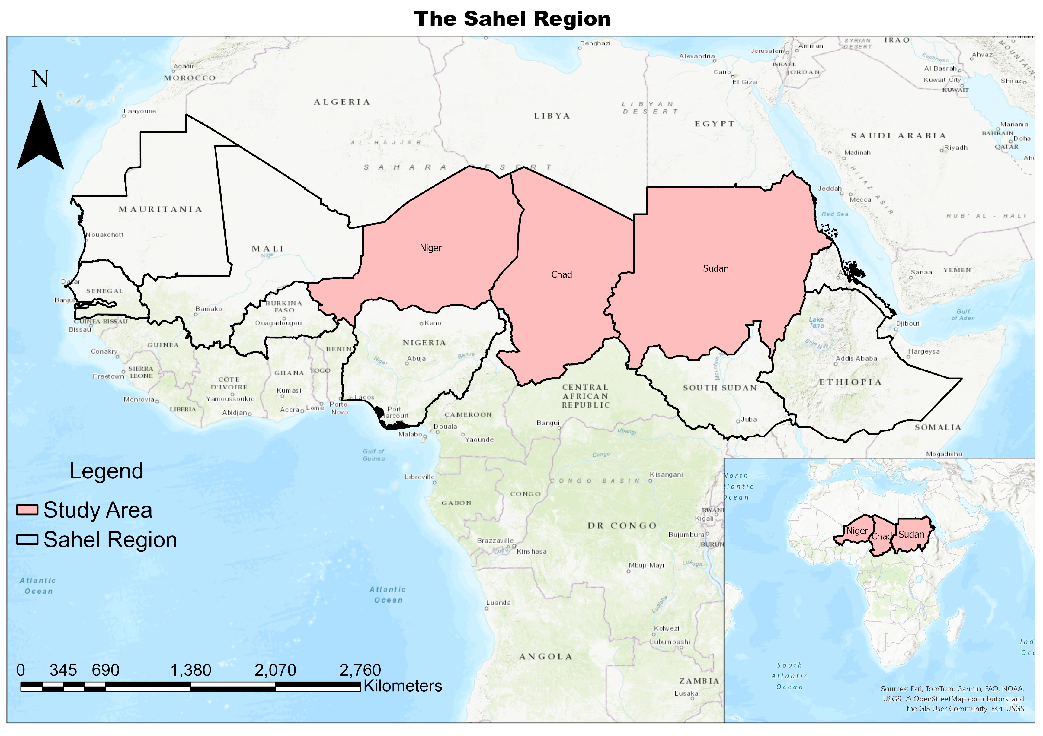
Figure 2.
Spatial Distribution of NPP in Chad, Niger, and Sudan (2019–2021).
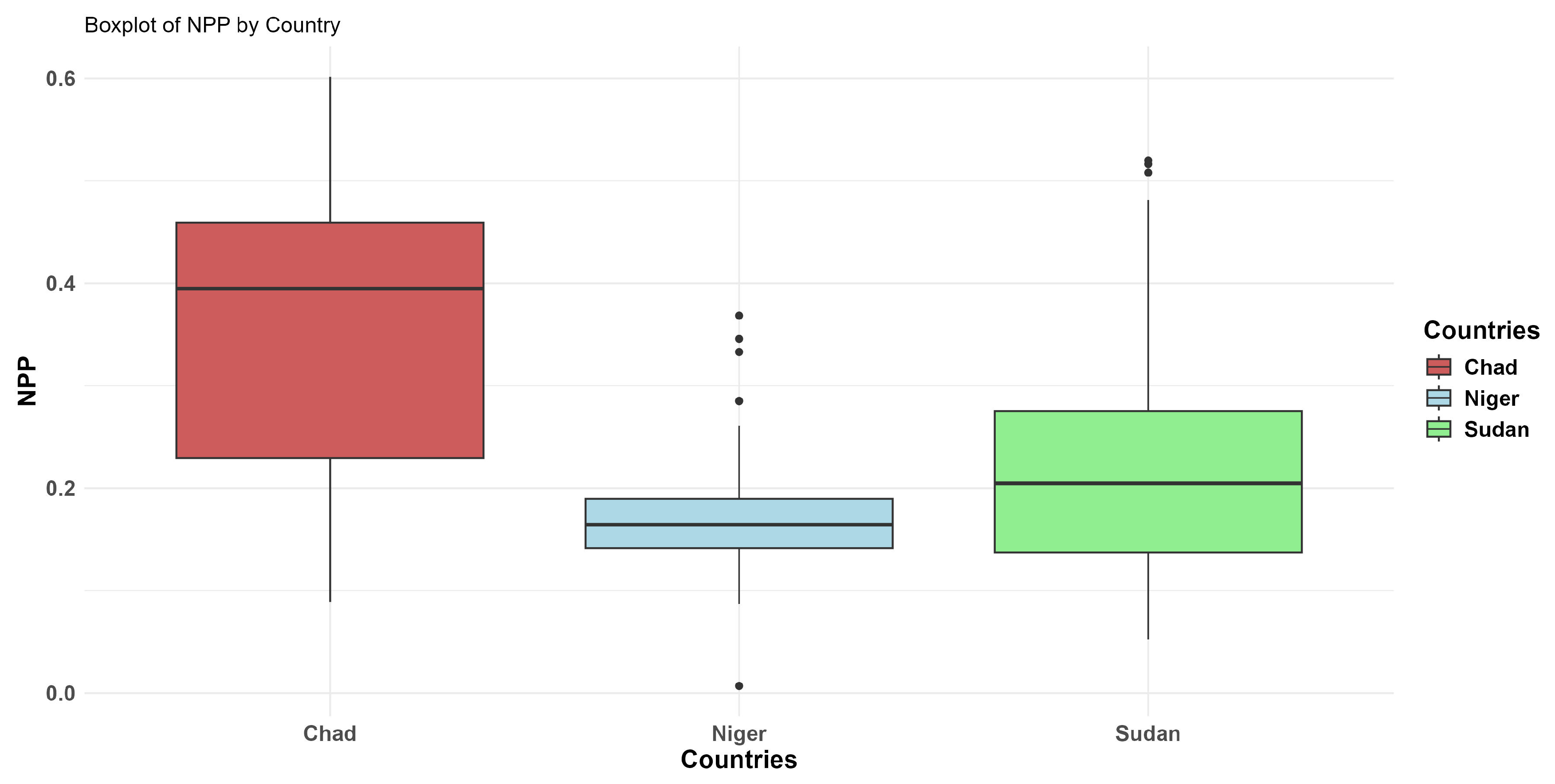
Figure 3.
Descriptive maps of NPP and its predictors.
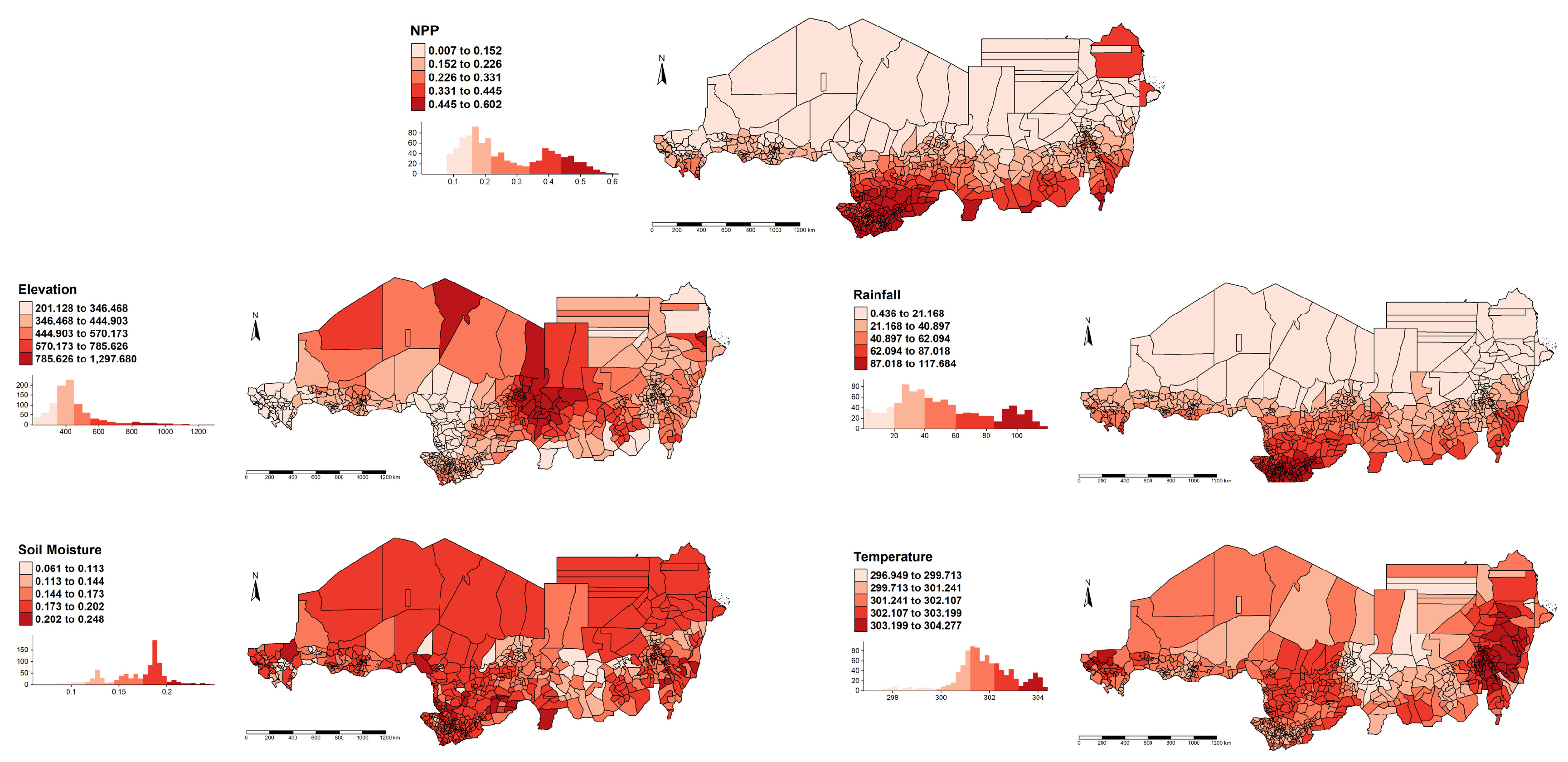
Figure 4.
Map of OLS Residual Distribution.
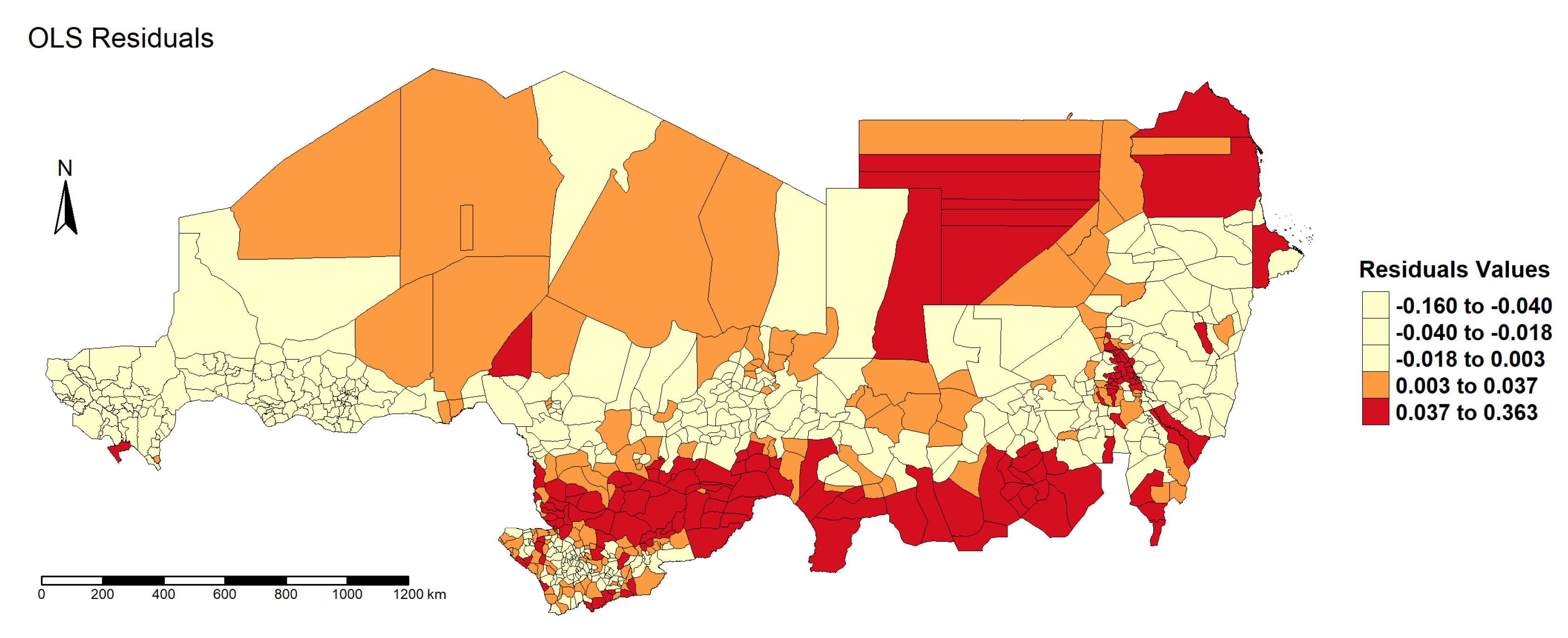
Figure 5.
Maps of the GWR Coefficient Estimates.
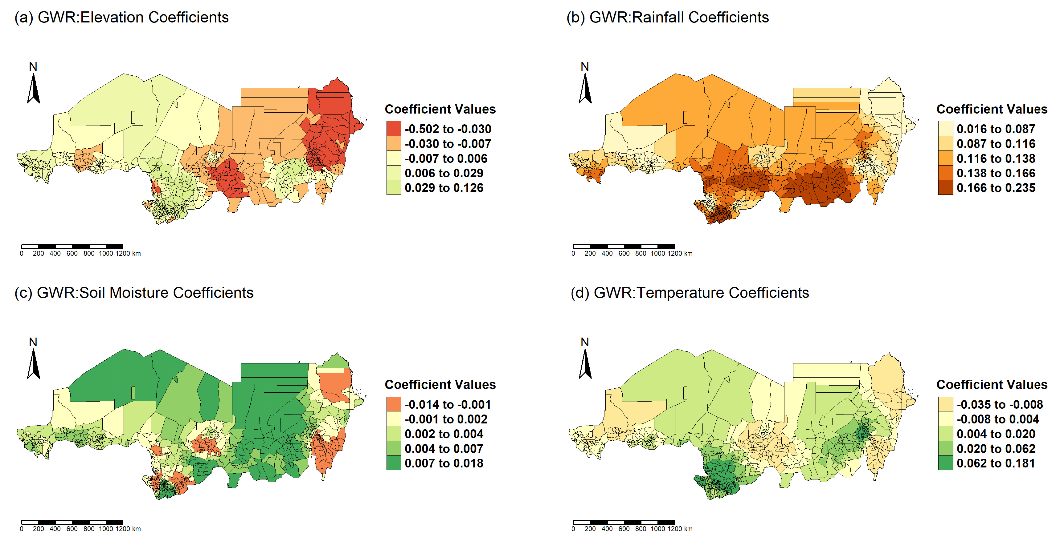
Figure 6.
Map of Values from the GWR Model.
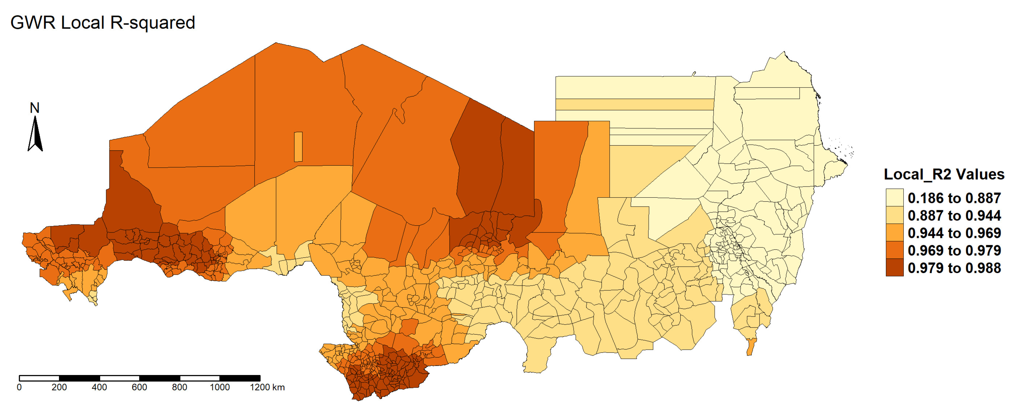
Figure 7.
Visualising Nonlinear Effects of Covariates with PDPs.
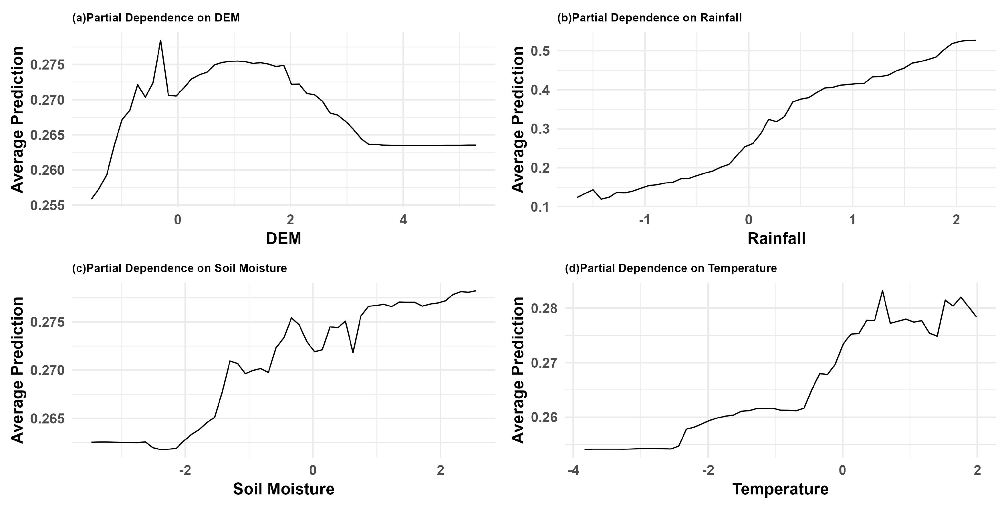
Figure 8.
Global Feature Importance (RF) and Mean Local Feature Importance (GWRF) Based on IncMSE.
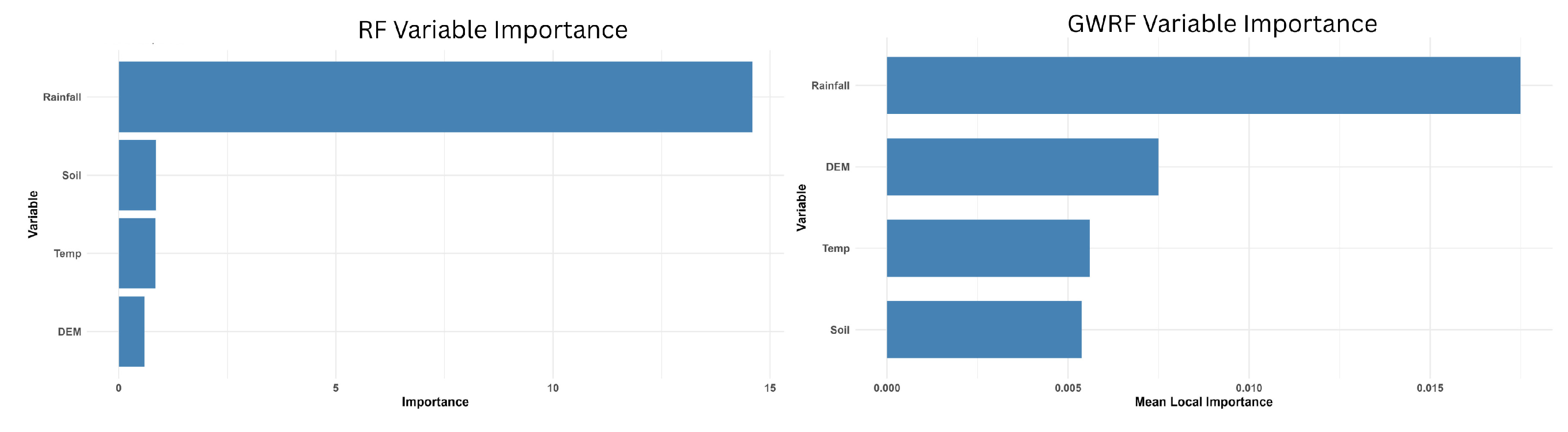
Figure 9.
Local Feature Importance Maps.
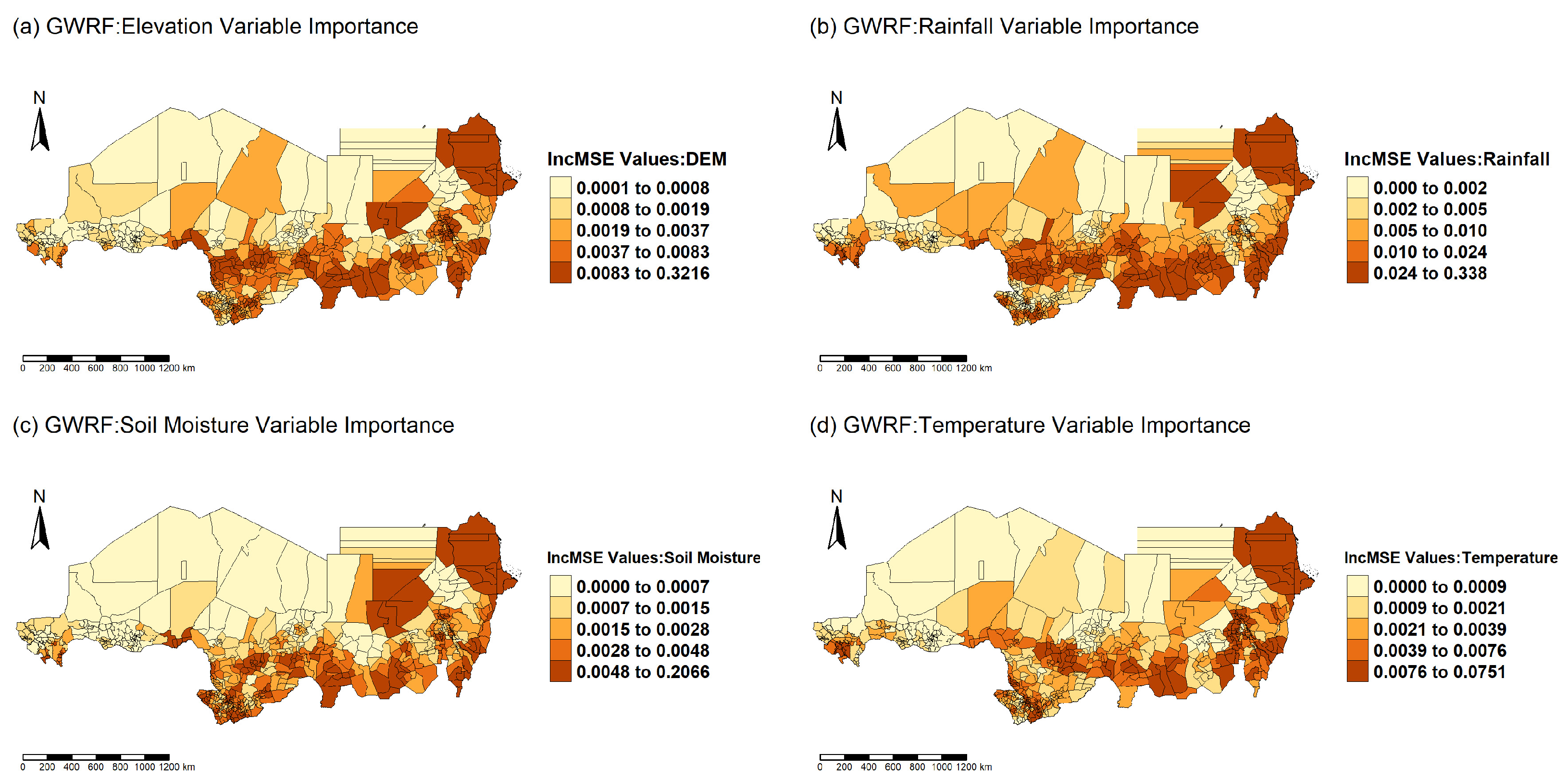
Figure 10.
Map of Values from the GWRF Model.
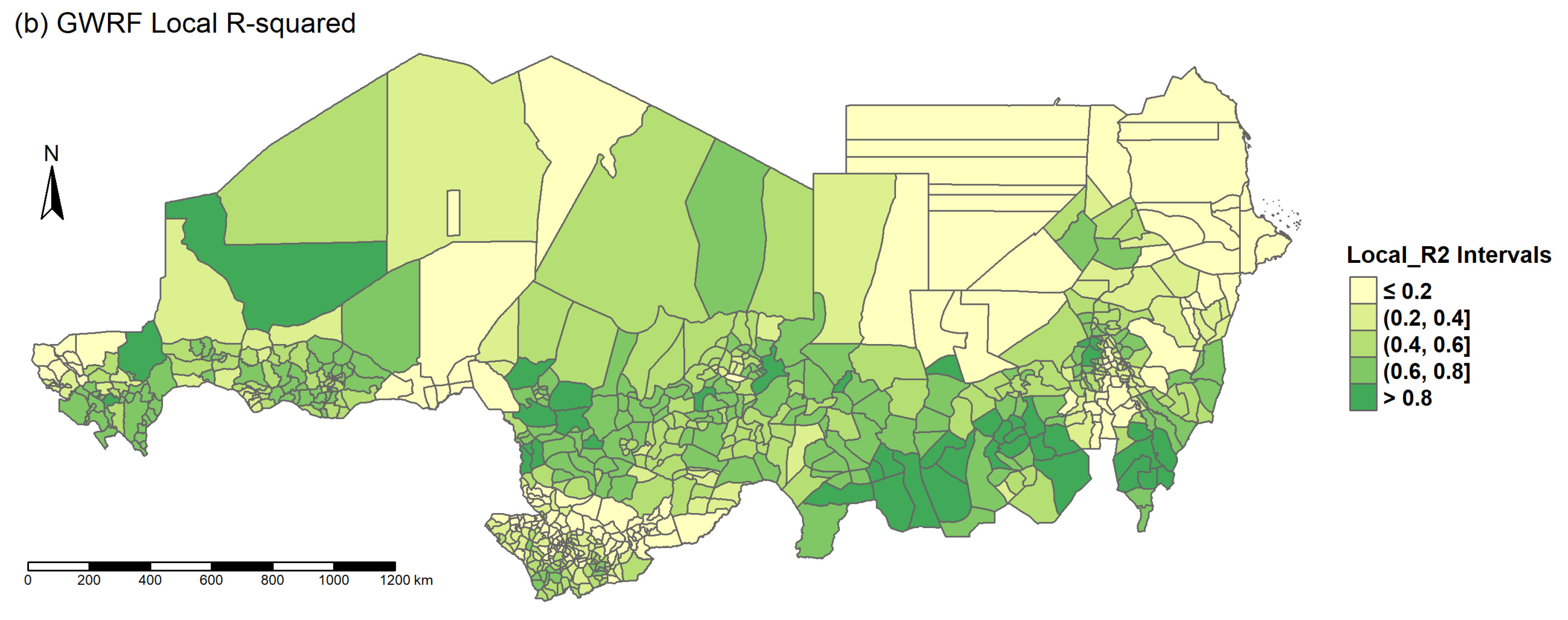
Figure 11.
Input to Hidden Layer Weights.
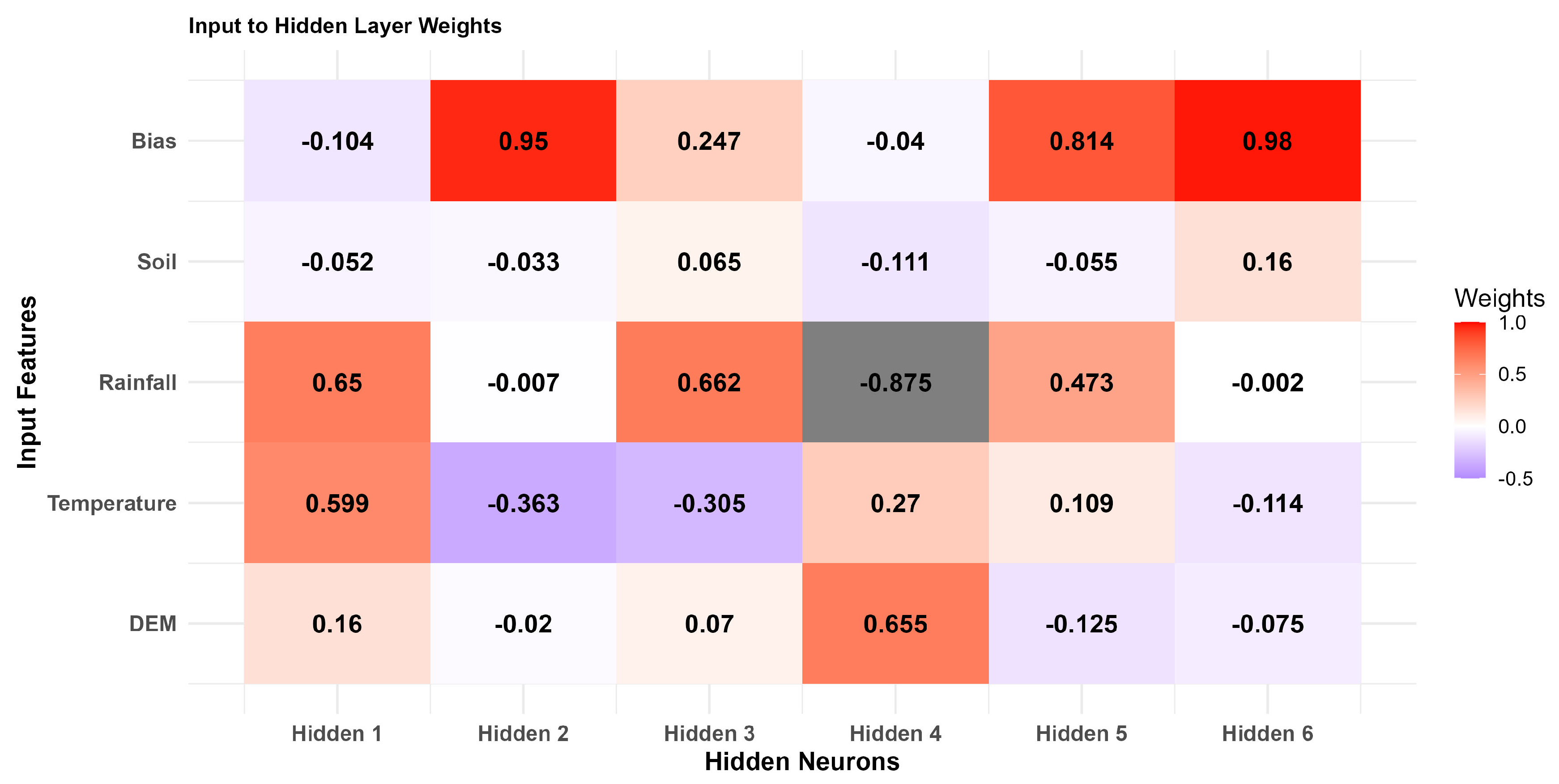
Figure 12.
GWNN Connection Weights (Hidden to Output Neurons).
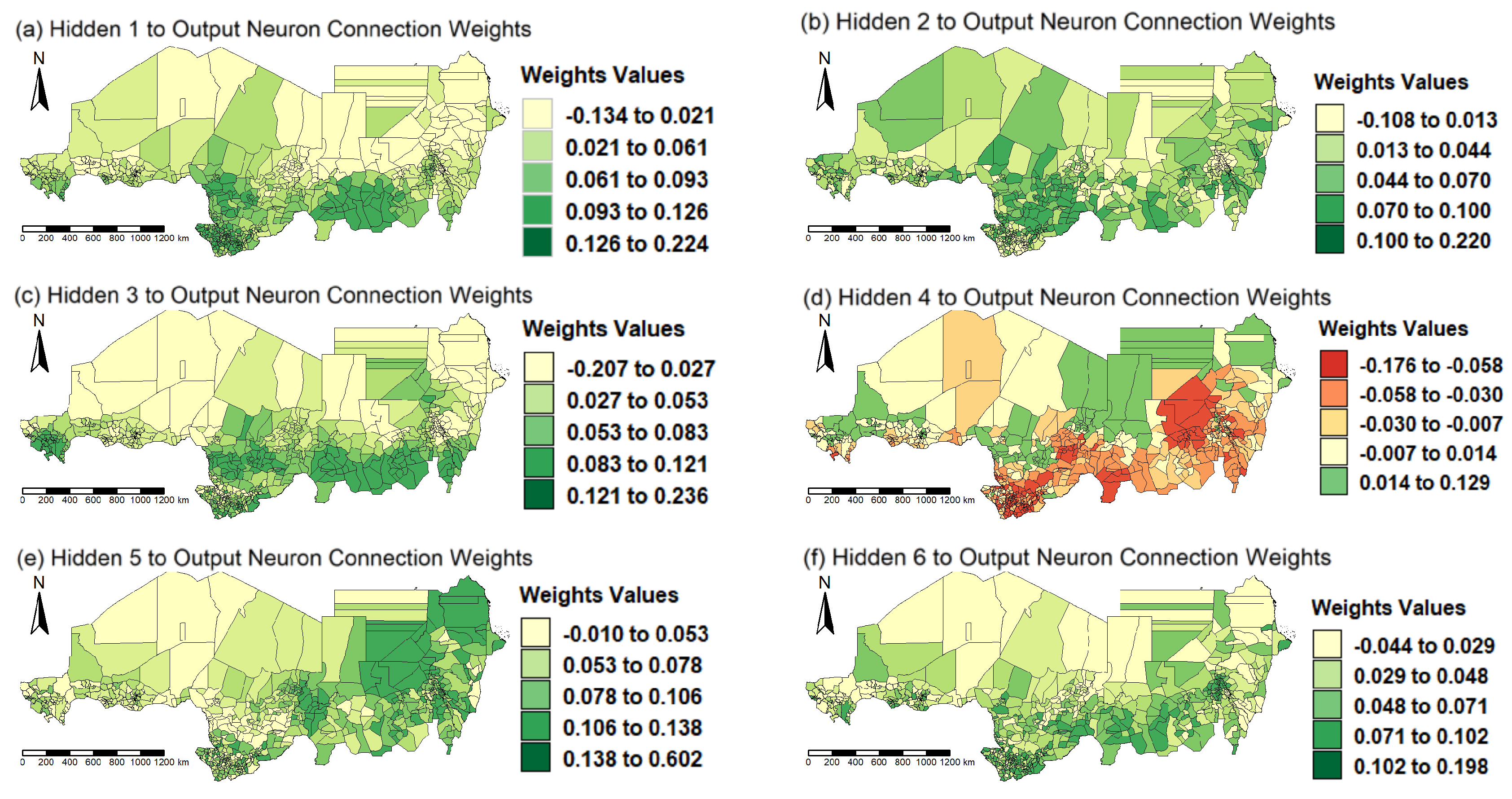
Figure 13.
Residual Mapping and Spatial Clustering (Local Moran’s I) for each Model.
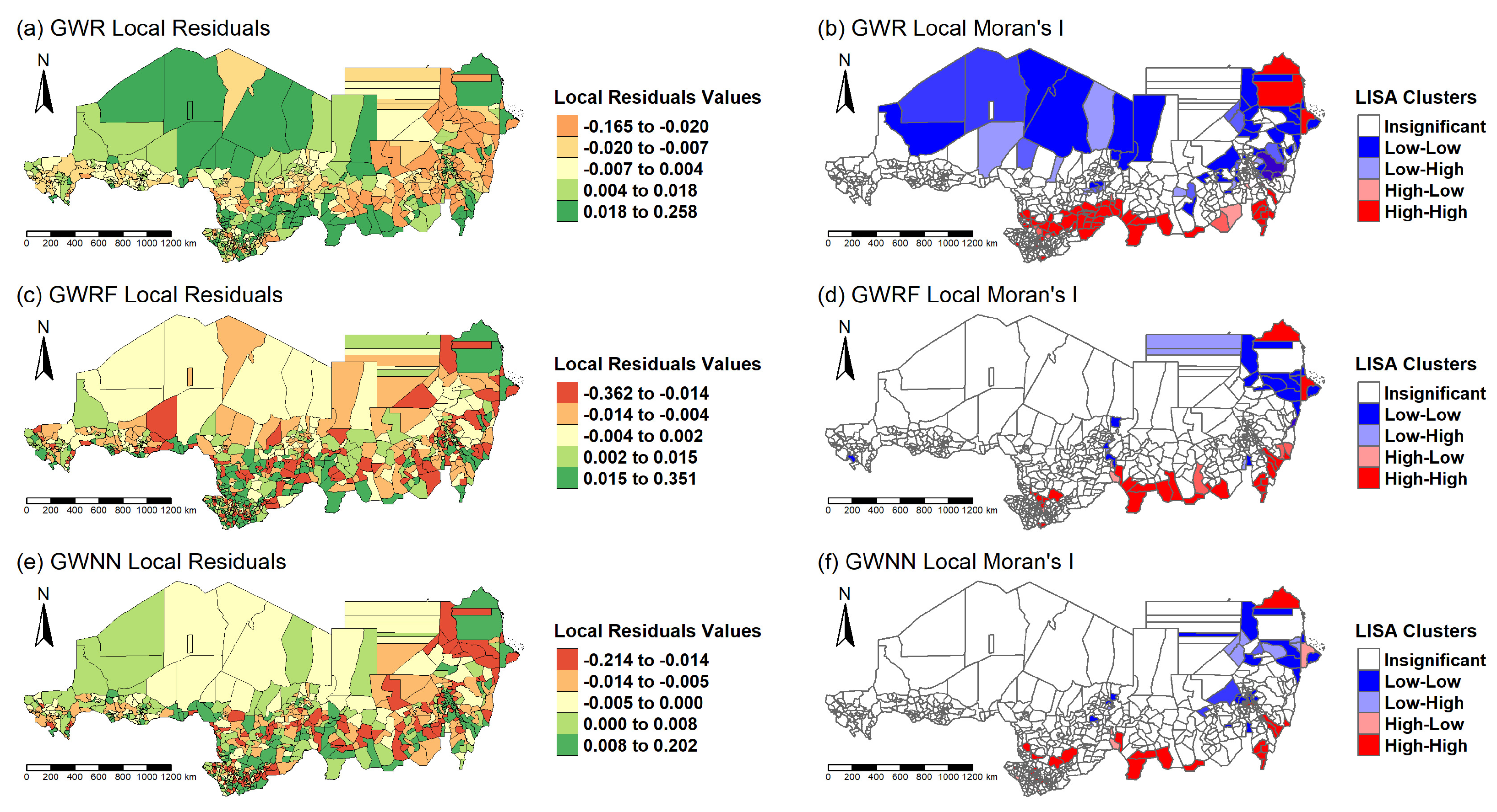
Figure 14.
The Scatterplots of Actual and Predicted NPP in 94 test samples for the OLS, RF, NN, GWR, GWRF, and GWNN Models, Respectively.
Figure 14.
The Scatterplots of Actual and Predicted NPP in 94 test samples for the OLS, RF, NN, GWR, GWRF, and GWNN Models, Respectively.
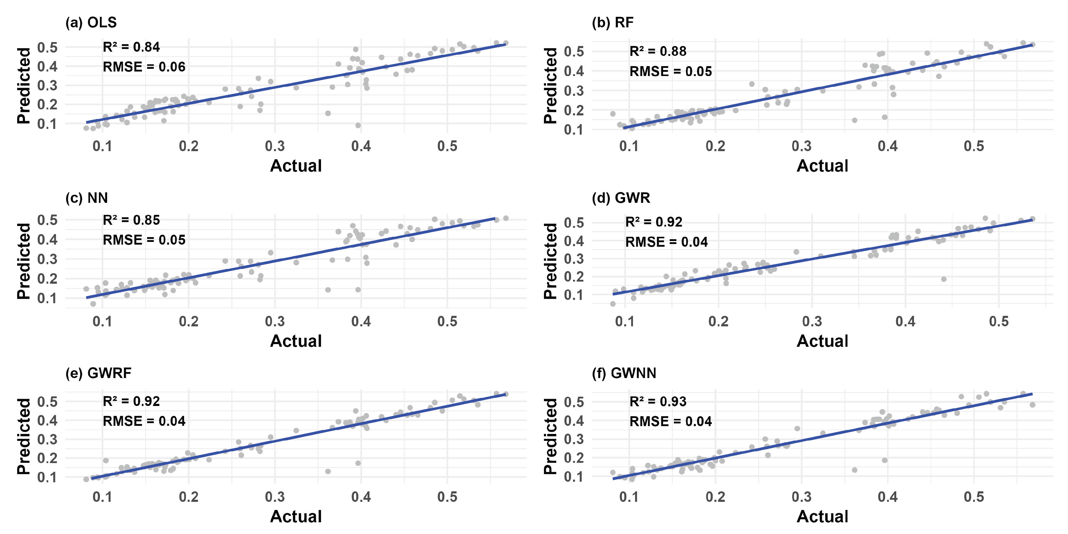

Table 1.
Datasets and Data Sources for Study Parameters.
| Data | Variables | Unit | Source | Format | Spatial Resolution |
|---|---|---|---|---|---|
| Climate | Rainfall | CHIRPS | TIF file (.tif) | ||
| Temperature | ECMWF | NetCDF (.nc) | |||
| Soil | Soil Moisture | ESACCI | NetCDF (.nc) | ||
| Topography | Elevation | SRTM | TIF file (.tif) | ||
| Vegetation Indices | NDVI | - | AVHRR | NetCDF-4 (.nc4) |
Table 2.
Missingness Percentage per Variable.
| Variables | Missing Value % |
|---|---|
| NDVI/NPP | 2.23 |
| Soil Moisture | 3.30 |
| Elevation | 7.03 |
| Rainfall | 0.00 |
| Temperature | 1.81 |
Table 3.
Summary statistics of NPP and environmental predictors.
| Variable | Min | Max | Mean | Median | SD |
|---|---|---|---|---|---|
| NPP | 0.006 | 0.602 | 0.272 | 0.228 | 0.135 |
| Soil Moisture | 0.061 | 0.248 | 0.169 | 0.181 | 0.031 |
| Elevation | 201.13 | 1297.68 | 447.12 | 411.36 | 160.69 |
| Temperature | 269.95 | 304.28 | 301.77 | 301.70 | 1.26 |
| Rainfall | 0.44 | 117.68 | 50.86 | 44.42 | 30.50 |
Table 4.
OLS Results.
| Variable | Coefficient | Std Error | t-Statistic | p-value |
|---|---|---|---|---|
| Intercept | 0.272211 | 0.001783 | 152.630 | < 2e-16 |
| DEM | 0.010649 | 0.002396 | 4.445 | 9.82e-06 |
| Soil | 0.012330 | 0.001880 | 6.559 | 8.96e-11 |
| Rainfall | 0.122999 | 0.002011 | 61.174 | < 2e-16 |
| Temp | 0.017131 | 0.002407 | 7.117 | 2.19e-12 |
| Adjusted | 0.8354 |
Table 5.
Coefficient Estimates from GWR and OLS Regressions.
| Min. | 1st Qu. | Median | Mean | 3rd Qu. | Max. | F3 Test (p-value) |
Global OLS |
|
|---|---|---|---|---|---|---|---|---|
| Intercept | 0.0304 | 0.2182 | 0.2703 | 0.2582 | 0.2965 | 0.4116 | 1.50e-152 | 0.272211 |
| DEM | -0.5019 | -0.0209 | -0.0001 | -0.0115 | 0.0194 | 0.1259 | 4.37e-139 | 0.010649 |
| Soil Moisture | -0.0136 | 0.0002 | 0.0027 | 0.0030 | 0.0063 | 0.0183 | 2.90e-10 | 0.012330 |
| Rainfall | 0.0155 | 0.0940 | 0.1279 | 0.1280 | 0.1583 | 0.2352 | 4.34e-146 | 0.122999 |
| Temperature | -0.0350 | -0.0055 | 0.0103 | 0.0260 | 0.0522 | 0.1815 | 2.62e-183 | 0.017131 |
Table 6.
Summary Results of RF and GWRF Models.
| RF | GWRF | ||||||
|---|---|---|---|---|---|---|---|
| Local Feature Importance (IncMSE) | |||||||
| Rank | Variable | Global Feature Importance | Variable | Min | Max | Mean | Std |
| 1 | Rainfall | 14.5951 | Rainfall | 0.3379 | 0.0175 | 0.0331 | |
| 2 | Soil Moisture | 0.8620 | DEM | 0.3216 | 0.0075 | 0.0212 | |
| 3 | Temperature | 0.8408 | Temperature | 0.0751 | 0.0056 | 0.0084 | |
| 4 | DEM | 0.5900 | Soil Moisture | 0.2066 | 0.0054 | 0.0173 | |
| 0.8985 | 0.9376 | ||||||
| MSE | 0.0018 | 0.001 | |||||
Table 7.
Missingness Percentage per Variable.
| The Local Value of | % of counties |
|---|---|
| ≤ 0.2 | 22.04 |
| (0.2, 0.4] | 16.30 |
| (0.4, 0.6] | 27.69 |
| (0.6, 0.8] | 27.26 |
| > 0.8 | 6.71 |
Table 8.
Global Moran’s I for Residuals of GWR, GWRF, and GWNN.
| Model | Global Moran’s I | p-value |
|---|---|---|
| GWR | 0.1750 | 2.2e-05 |
| GWRF | -0.0352 | 0.9958 |
| GWNN | -0.0004 | 0.4810 |
Table 9.
Comparison of Models’ Performance on the Test Dataset using Cross-validation.
| OLS | RF | NN | GWR | GWRF | GWNN | |
|---|---|---|---|---|---|---|
| MSE | 0.0030 | 0.0018 | 0.0023 | 0.0015 | 0.0013 | 0.0012 |
| RMSE | 0.0542 | 0.0429 | 0.0474 | 0.0371 | 0.0337 | 0.0333 |
| MAE | 0.0392 | 0.0270 | 0.0324 | 0.0243 | 0.0191 | 0.0205 |
| 0.8378 | 0.9008 | 0.8755 | 0.9207 | 0.9308 | 0.9360 |
Disclaimer/Publisher’s Note: The statements, opinions and data contained in all publications are solely those of the individual author(s) and contributor(s) and not of MDPI and/or the editor(s). MDPI and/or the editor(s) disclaim responsibility for any injury to people or property resulting from any ideas, methods, instructions or products referred to in the content. |
© 2025 by the authors. Licensee MDPI, Basel, Switzerland. This article is an open access article distributed under the terms and conditions of the Creative Commons Attribution (CC BY) license (http://creativecommons.org/licenses/by/4.0/).
Copyright: This open access article is published under a Creative Commons CC BY 4.0 license, which permit the free download, distribution, and reuse, provided that the author and preprint are cited in any reuse.


