Submitted:
18 November 2025
Posted:
19 November 2025
You are already at the latest version
Abstract
Since its inception, Quantum Mechanics (QM) has engaged many philosophers the subspecialty of a few. More recently, QM has attracted the attention of a few neuroscientists modelling neuronal and higher brain function. This pedagogical review aims to make QM more accessible to neuroscientists and philosophers less familiar with its basics. Emphasis is on QM measurement and entanglement. We write at an intermediate technical level between elementary textbooks and contemporary journals. Against authoritative advice, we use the “crutch of visuality” to ease comprehension of notoriously difficult ideas in QM, e.g., complex Hilbert space, an apparatus setting the outcomes of an experiment. To keep more advanced readers interested, we sow philosophical comments throughout the text. These touch on under-discussed themes (e.g., complex numbers in QM), seek to clarify pedagogically neglected matters (e.g., particles of definite energy), and strike occasional possibly novel points about QM (e.g., the metaphysical double-humility of QM, the quantum state as an ontologico-epistemological hybrid). We strive ultimately to show that even orthodox QM is more concretely graspable and philosophically better thought-out than many have judged.
Keywords:
measurement problem
; quantum entanglement
; foundations of quantum mechanics
I. Introduction
From the beginning, Quantum Mechanics (QM) has nourished physicists conjecturing about philosophy and philosophers delving into physics (e.g., Heisenberg 1955; Jammer 1974; Popper 1982; Halvorson 2011,2019; Carroll 2017, Myrvold 2022; Muller 2023). More recently, neuroscience has explored QM for modelling in order to model neuronal physiology or higher brain functions (e.g., Beck 1996, Hameroff & Penrose 1996ab, Schwartz et al. 2004, Ivanov & Schwartz 2018, Mitchell 2023). This pedagogical review aims to make QM more accessible to neuroscientists and philosophers less familiar with its basics. Emphasis is on QM measurement and entanglement. We write at an intermediate technical level between elementary textbooks and contemporary journals. Knowledge of mathematics is presumed up to linear algebra and differential equations, but only elementary physics. Against the advice of some respected teachers of QM, we use the “crutch of visuality” (Boyer 1968) to ease comprehension of certain notoriously difficult ideas in QM. To sustain the interest of more advanced readers, we have strewn philosophical comments across the text. These touch on under-discussed themes, seek to clarify pedagogically neglected matters, and strike occasional possibly points about QM we have not previously encountered. We strive ultimately to show that orthodox QM is less mysterious and more concretely graspable; nor is it an ad hoc explanation of empirical findings , but it is philosophically better thought-out than many have judged. (Note: in this text we abbreviate both the noun “Quantum Mechanics” and the adjective “quantum mechanical” with “QM”; likewise for “Classical Mechanics”; “classical mechanical” and “CM”.)
II. Measurement
A. Particles
1. Single Particle. The model quantum system in this paper is a single particle. Single particles are easy to work with and single-particle results are readily extended to multi-element systems. Hence, much of what we say in this paper about a “particle” applies to quantum systems more widely. Although we seldom identify the species of particles in this text, note that every particle belongs to one species or another. The species may be elementary, e.g., an electron or photon, or composite, e.g., a hydrogen or fluorine atom. The species sets the degrees-of-freedom per particle, the number of different ways the particle can store and transfer energy, momentum, angular momentum,… It equals the number of independent quantum states per particle. The latter fixes in part the dimension (number of independent axes, size of the basis) needed to generate the state space or Hilbert space of a quantum system. We discuss these concepts below.
2. CM Waves and Particles. QM “particles”, notoriously, act at times like CM particles, at times like CM waves. Regardless of size, a CM particle can be treated formally as if it occupied a single point in space at each instant in time. That point, for massive (i.e., non-zero mass) particles, is its center-of-gravity (c.g.) A CM particle travels thru space-time in a 1D trajectory with one velocity at each point along the trajectory. When two particle trajectories intersect, the particles often simply bounce off each other, preserving their integrity thereby. (They may also undergo a chemical, nuclear,… reaction, transforming into different species.) In sum, classical particles are hard, compact entities like bullets, pebbles, or seeds that hold together, resist combination, and move on well-defined paths.
Structure and behavior of a CM wave, in contrast, are never captured by a single point. A wave rather spreads (Figure 1), often in rhythmic peaks and troughs, across space and time. Its wavelength is the scale of spread in space, its frequency the scale of spread in time. Instead of trajectories, waves travel in 1D or 2D wavefronts. Waves, moreover, have two velocities. Wave group velocity is the rate at which single pulses (contiguous feature aggregates) of the wave, wave groups or wavepackets, propagate thru space. is also the velocity of the wavefront and of the envelope surrounding a wavepacket. Phase velocity is the rate at which any single feature (e.g., the crest of one peak) moves within or between wave groups. For monochromatic (single-wavelength, single-frequency) electromagnetic waves (light) and , where is the speed of light in vacuum and light-speed in any particular medium. When waves collide they do not preserve their integrity. Rather, they merge, they superpose or interfere. When waves merge, their coincident amplitudes add algebraically point-by-point. Positive adds to positive to make higher peaks; negative adds to negative for deeper troughs (constructive interference). Positive and negative aligned amplitudes, however, wholly or partially cancel each other out (destructive interference). Constructive and destructive interference can result in complicated waveforms with multiple frequency components. Critically, constructive can become destructive interference (and vice-versa) when a (left or right) phase shift of one or both summing waves turns peaks wholly or partly into troughs (and vice-versa). Hence, the (leading or lagging) phase determines the outcome of superposition independently from and as much as intrinsic variation in the (positive or negative) wave amplitude. In sum, we think of waves as fusible, diffuse entities like swell on the beach, audio tones, or mechanical vibrations that dissipate, readily combine, and propagate in fronts.
3. Complex Numbers. Both CM and QM waves are well modelled using complex numbers. Complex numbers are widely used in Physics in scenarios where two independent algebraically signed factors (like phase and amplitude of a wave) determine an outcome. In CM, complex numbers are a mathematical convenience. In QM complex numbers are undeniably indispendable in everyday practice. One debates whether they are ultimately just mathematical tools or of deep significance. This subsection detours briefly from the main theme to introduce complex numbers and to motivate their use.
As neuroscientists know from MRI and elsewhere, a complex number is a number of the form (). is the base of the imaginary number system. In polar form, a complex number is . The norm, length, magnitude, or modulus of is . Every complex number has a conjugate, , formed by replacing wherever it appears by . has the same length as , . A related expression much used in QM is . (In general .) Complex numbers can be represented as vectors on the complex plane with the real axis serving as and the imaginary as . A limitation to this analogy is that one can divide by any non-zero complex number , but never by a 1D number-array vector.
Hard-headed people ask, “How can a number be imaginary!? What’s that supposed to mean!?” Here is one answer, a way to intuit complex numbers in physics. Complex numbers are often used in CM scenarios where some quantity (charge, energy,…) shuttles periodically between two independent modes. One mode is assigned to the real, the other to the imaginary axis. Complex numbers are used when the real axis alone is insufficient to keep track of everything that is going on with a phenomenon.
As example, take a series AC electrical circuit. The circuit is driven by a power supply or other source. It generates, as they typically do, an AC voltage that varies in time as a complex sinusoid, e.g., . (A “sinusoid” is a function from the family of constant, trigonometric, exponential, or related functions.) is the maximum amplitude of the signal and its frequency. The source is attached to a resistor , a capacitor , and an inductor all connected in a row. If we attach the twin leads of a voltmeter across it measures the real part of the voltage . ( is called the dissipative component of the circuit since it dissipates the electrical energy put into it by the source immediately.) If we place the leads across together the voltmeter measures the imaginary part of the voltage . ( is the reactive component; it reacts to input energy by storing it temporarily. stores magnetic energy on the timescale ; stores electric energy on the timescale .) Since , both real and imaginary parts oscillate smoothly between and . The magnitude of the total voltage remains constant as it shuttles between positive and negative real and imaginary components. At , the full voltage is across ; the voltage across is 0, it only exists in potentia. But later, at , the voltage is 0 and only exists in potentia while the voltage is . Later still, at , the situation again reverses. For a metaphysical perspective related to QM, suppose is very low, the circuit oscillates so slowly you can touch it and pull back before the voltage changes much. If you grabbed the resistor bare-handed and grounded at when its voltage was near zero, you’d feel nothing. Very little voltage would be in the real mode. Most would be imaginary. It would not yet be part of reality for you. But if you hung on, by the voltage would be fully back in the real mode and shock you! Hence, imaginary numbers have real consequences. Intriguingly, you might never feel the shock, e.g., if someone cut the wire before the heavy voltage hit. In that sense, the potential voltage in the imaginary mode is not real. In the normal course of events, however, eventually the voltage will rise and shock you if you don’t let go. Endlessly many physical events in the world run similar cyclic courses. Thus, effects represented by imaginary numbers do exist in a pragmatic sense. They reflect what can and usually does happen. The same hard-headed soul who scoffed at imaginary numbers would be the first to scold you for playing with live wires!
Complex numbers show quantitative linkages between physical modes in space and time. An element of time is inevitably present in practical measurements. Even flash photography requires non-zero time to register an image. As ultra-precise as time metrology has become, physics still cannot eliminate time from its models. Complex numbers are highly apt for capturing, especially rhythmic, variations of CM quantities in time. In QM, the probability amplitude (see below) for observing a particle in a certain quantum state may act like a vector of constant length rotating rhythmically around the complex plane. One interpretation of this is that particle properties (like voltages in AC circuits) oscillate in and out of reality. An alternative, holistic, interpretation is that QM information is shuttled between one mode for information manifest by a single particle and another for information banked in in the statistical ensemble to which the particle belongs.
4. Dual-Slit Experiment: Wave-Particle Duality. Feynman (e.g., Feynman & Hibbs 2010) famously used the Dual-Slit Experiment to illustrate Wave-Particle Duality and the need for complex numbers in QM. We discuss this briefly for the case of electrons (Figure 2; Jönsson et al. 1961). With parameters modified, similar results are obtained for all QM particles, including photons (Young 1804), neutrons (Zeilinger et al. 1988), atoms (Carnal & Mlynek 1991), even buckyballs (Arndt et al. 1999)! In the Dual-Slit Experiment, an electron gun fires electrons thru one or both of a pair of identical narrow (even for an electron) vertical slits (A,B) cut in an otherwise impermeable thin partition. (Either the gun slides horizontally on a track to line-up in the middle or behind either slit or the dimensions are so small the gun need not move.) The horizontal gap between the slits is modestly wider than the slits themselves. Slit height can be taken as infinite. A screen mounted ~1 m opposite registers the impact of each electron making it thru the slit and across the distance. After firing many electrons, the impacts form a spatial pattern or distribution across the screen. The horizontal () component of the distribution is of prime interest. , the number of impacts at each in a given time interval is proportional to the electron beam intensity and to the probability of an impact at . If we run the experiment with A open and B covered or vice-versa (single-slit paradigm), we get the distributions , respectively, . If we open both slits (dual-slit paradigm), we get .
First we observe that, no matter which slit(s) are open, we always detect individual electrons impacting at the screen. (As implied above, the same happens when one does the experiment with light, individual photons are registered at the screen.) This suggests electrons (and photons, etc.) are discrete CM particles. This conclusion, however, is contradicted by the mathematical form of the distributions , , and . If electrons were CM particles, would be a flat line segment of constant height and width located directly across from A and aligned with it. Outside this segment, the probability of observing an electron impact would be 0. The same curve would result for , only shifted to the right to align with B. would consist of both segments side-by-side, separated by . In reality, and are not constant functions, but given by
Single-Slit Diffraction Probability Distributions
where is the maximum electron wave amplitude. (Other symbols defined in text and Figure 2). These are variants of the sinc function (). The maxima of these distributions do occur opposite their respective slits, yet many electrons impact left and right of the slits. The distributions are a kind of diffraction pattern. Diffraction is typical behavior for several kinds of CM waves. It results from the bending of a wave as it passes thru an aperture, like Slits A and B. is a more complicated sinc
Dual-Slit Diffraction Probability Distribution
It indicates diffraction combined with interference (Figure 1). It suggests that electrons emerge from A and B as coincident waves that interfere with each other constructively and destructively as they propagate to yield peaks and troughs at the target. This is again CM wave behavior. Thus, , , and suggest electrons are CM waves. Hence, the Dual-Slit Experiment provides clear evidence that electrons (and other QM particles) act sometimes like CM waves and sometimes like CM particles.
Now, for water waves, the level of the water surface is the quantity bobbing up-and-down. For sound waves, it is the air pressure level. In AC circuits, it is voltage or current. If we say that QM particles act at least partly like CM waves, what exactly is waving for a QM particle? In >100 years, QM has still not answered this question satisfactorily. Since Eqs. (1-2) are for probabilities, perhaps QM waves are probability waves? This, however, is not quite accurate. If electrons moved in probability waves, for both slits open the distribution would be simply (Figure 2 teal). But the actual distribution . These quantities cannot be equal. For probabilities are always positive numbers. Adding them could never generate the troughs in the interference pattern. The electron wave is instead a probability amplitude , a complex number that, multiplied by , is proportional to a probability, e.g., , . For both slits open, . Only by adding and as complex numbers can we reproduce the empirically observed interference pattern. Thus, the Dual-Slit Experiment shows the necessity of complex probability amplitudes to describe QM particles.
A couple remarks on Wave-Particle Duality. The wave properties of QM particles have statistical character. That is, they emerge when large numbers of particles are observed. If we run the dual-slit paradigm and place two additional detectors right in front of A and B, we always see a single electron emerge from one or the other slit, as if the electrons are acting like CM particles. I.e., we never see the electron split half going thru each slit. But without the extra two detectors and examining large numbers of electrons, the screen impacts always distribute themselves in an interference pattern. It is as if the electrons were diffracting as they passed thru each slit and interfering with themselves as they passed thru both slits, in the manner of CM waves. Amazingly, this happens even if the electrons are fired one-by-one, hours, even days apart! I.e., results are unaffected by the mere passage of time. In QM, all particles act like waves for certain measurements and like particles in certain other measurements. As Feynman explains, whenever there are exclusive alternative paths available to a QM particle, e.g., when we can know with certainty the electron has gone thru A or B, we see particle behavior. Whenever we have interfering alternative paths, e.g., we cannot know whether the electron has gone thru A or B, we see wave behavior. Note that it is not about what we do or do not know in a particular instance, it is about what we fundamentally can or cannot know, given the paradigm. Intriguingly, quantum systems never exhibit both wave- and particle-character in the same measurement. Perhaps this is a consequence of the way experimental designs make sharp distinctions between what can and cannot be known. Finally, one is not restricted to two vertical slits, one may carve apertures of any shape and size into the partition and measure the resulting impact distributions. A deep insight is that the diffraction pattern is, in general, the complex Fourier Transform of the aperture function (the shape and size of the aperture across ).
5. Consequences of Wave-Particle Duality. We present two key consequences of Wave-Particle Duality.
The first is the Planck-Einstein Quantum of Action
Planck-Einstein Quantum of Action
Eq. (3) gives the total energy of a single QM particle (especially of a photon of monochromatic light). The higher the particle frequency , the greater its energy. is Planck’s constant, a universal constant of Nature central to QM. Among other things, multiples of (the reduced Planck’s constant ) represent the quanta (smallest possible amounts in Nature) of angular momentum (torque or “rotational force” applied over time) or of action (energy applied over time). Eq. (3) reflects the particle-character of QM particles. Thus, energy and angular momentum come in packets (particles) of a minimum size.
The second result is the de Broglie Hypothesis. Although their mass is zero, photons have not only energy, but also linear momentum . The latter is given by
de Broglie Linear Momentum of a QM Particle
Thus, the longer the wavelength, the smaller the momentum; the shorter the wavelength, the greater the momentum. In a revolutionary departure from CM, the de Broglie Hypothesis also applies to massive particles, e.g., electrons, protons,… A particle of mass moving at velocity has (non-relativistically) momentum . Per Eq. (4), every such particle has a wavelength . (Note that here is the group velocity of the particle wave.) QM experiments consistently show that light acts like particles with energy given by Eq. (3) and momentum given by Eq. (4). Further experiments confirm that massive particles like electrons, neutrons, etc. have wavelengths given by Eq. (4) and can be focused, refracted, diffracted, etc. just like light waves.
B. Quantum System
1. Irreducibility. We seek here a definition of a quantum system better than those usually offered. A common strategy is to define quantum systems as “microscopic” in scale and to contrast them with the “macroscopic” systems of CM. While quantum systems usually are microscopic, macroscopic quantum systems do exist, e.g., superconductors and superfluids (Annett 2005). Moreover, the formal boundary between macro- and microscopic is challenging to nail down (Jaeger 2014). An alternative is to oppose “discrete” quantum systems to “continuous” CM systems. But continuous systems abound in QM. The free particle, for example, adopts continuous values of position, momentum, energy,… And when discrete energy levels, e.g., the electronic orbitals of an HI molecule, do exist in quantum systems they may arise from (often CM-defined macroscopic) boundary conditions (BCs) imposed upon the system, rather than from quantum character per se. Many CM systems, furthermore, are discrete, e.g., the tones of a violin string or pipe organ. So neither of these approaches works well.
A superior option is to denote a quantum system as a physical system treated irreducibly, i.e., independent of internal dynamics (Carcassi & Aidala 2020). Internal dynamics are ignored because they are impossible, impractical, and/or inconvenient to ascertain. Nor would it relevantly alter results if we did include them. For example, it is still unknown if the electron possesses a non-zero radius or any substructure. (Its radius, if it does exist, is <10-22 m; Dehmelt 1988). Fortunately, outside, e.g., subspecialties in condensed matter physics (Yarris 2006, Schubel 2010), such putative substructure does not affect findings. In near-universal practice, therefore, one makes no effort to “look inside” the electron for factors influencing behavior. Its actions, rather, are ascribed wholesale to a single QM wavefunction (see below). As a second example, the proton does have well-accepted (albeit unobservable) subparts (two up, one down quarks). Nonetheless, the subparts are routinely ignored in molecular physics, chemistry,… Instead, one treats the proton to great effect as irreducible, with a single wavefunction. That is the quantum approach. As discussed elsewhere (O’Neill & Schoth 2022), it is similar to the way Computer Science seeks no substructure inside a bit. One accepts a bit as 0 or 1 and moves on. The same is done in endless many everyday tasks. Counting, e.g., apples tossed into a basket, we count each as “1” ignoring small differences from one apple to another (unless one is out-of-bounds, e.g., rotten, half-eaten, etc.) The word “quantum” means “quantity” or “number”. and other physical quanta are the numbers Nature counts with. She does this on successive levels of organization: A wavefunction for each quark, then one for the proton, one for the whole nucleus, one for the whole atom,… on up to the macroscopic. Generally, QM treats entities as countable, but indistinguishable, ignoring differences between them below a certain level of detail. The next subsection lists more formal specifications for a quantum system.
2. QM Laws. Characteristic of quantum systems is that we cannot measure all their physical properties together with unlimited precision (Heisenberg Uncertainty Principle). Moreover, we cannot predict measurement outcomes on these systems with certainty. We can only predict outcomes as probabilities of the results of numerous, repeated experiments. Foundationally, a quantum system is an irreducible system that obeys the following Laws: 1) The state of the system (quantum state) is represented by a complex-number vector (or function) in a Hilbert space; 2) The isolated state evolves in time according to the Time-Dependent Schrödinger Equation. Solutions to this equation are probability-amplitude waves. As waves, quantum states exhibit wavelike behaviors such as complex interference and superposition; 3) Each observable (measurable physical property) of the system is represented by an Hermitian operator that spans the Hilbert space; 4) The act of measuring any observable shifts the system into one of the multiple eigenstates of the corresponding operator, chosen at random. The measured value of that observable is the (always real) eigenvalue of that eigenstate; and 5) The probability of measuring the eigenvalue is calculated as follows: Take the (normalized) quantum state vector before the measurement, project it onto the post-measurement eigenstate, then multiply it by its own complex conjugate. The foregoing physicomathematical mumbo-jumbo is explained below.
Comment 1: A particle can be conceived of as a “carrier of degrees-of-freedom” (O’Neill & Schoth 2022). Degrees-of-freedom are familiar to neuroscientists from statistics. In physics, they are independent modes for storing energy, momentum, etc. Suppose, for example, our particle is a heteronuclear diatomic molecule, e.g., HI. HI has numerous such modes: One for translational kinetic energy (movement of the particle c.g. in an arbitrary external coordinate system), two modes for rotational kinetic energy (for joint rotation of the nuclei around any pair of perpendicular axes thru the c.g.), one for vibrational kinetic energy (joint oscillations of the nuclei along any axis thru the c.g.), electronic modes for the electrons, nuclear modes for the nuclei, etc. We can invest energy into (or withdraw it from) the molecule in all these modes. Energy is thereby both conserved and, like money, fungible, i.e., it interconverts freely between modes. Moreover, a particle takes its energy with it wherever its c.g. goes. And it retains the modes even when vacant; they travel with the particle waiting to be populated. (Since the modes derive from the particle quantum state, this fact supports the highly debated notion that quantum states have independent physical existence.) When the modes are populated, the particle holds onto the energy. It keeps it at and around its c.g., for some stretch of time. The time is longer for stable modes, e.g., ground-states; shorter for unstable modes, e.g., excited states. Hence, particles make available distinguishable modes of energy transfer and storage, localized in space and time.
Comment 2: Notoriously, the Second Law of Thermodynamics inexorably and ubiquitously drives natural processes towards a uniform distribution of energy across the Universe, an ahistorical state of thermodynamic equilibrium. Particles both mediate and hinder this process. I.e., they influence the rate at which it transpires. Suppose, for example, our HI molecule is carrying excess energy in an excited-state electron. Per the Second Law, probability favors (but does not compel) decay of that electron to the ground state. Upon decay, it emits the excess energy in a massless photon. Unbound, the photon flies away, spreading the energy to great distances at the fastest speed in Nature, . But if the electron does not decay, the energy remains bound in the molecule, a massive particle. The energy then spreads at more modest speeds, e.g., ~400 m/s at atmospheric pressure and room temperature. In this way, particles are one manifestation of reactive (time-dependent) effects in Nature. As in CM, the mass of the particle is its inertia, its tendency to stay at rest or moving on track against outside forces. Massive or not, particles have a dual role with regard to cosmic evolution. On the one hand, by distributing energy they help bring about the thermodynamic “End of History”; on the other hand, they preserve history, thru such details as the angle of emission of a particle escaping an atom. As particles interact, certain details become lost, but, for the Universe as a whole and for isolated local systems, certain constants-of-motion (energy, momentum, angular momentum, electric charge) are preserved under Conservation Laws no matter how complicated the interactions.
C. Heisenberg Uncertainty Principle
1. Supermicroscope Gedankenexperiment. This Gedankenexperiment (thought experiment; Figure 3) is overused and has been critiqued. Nonetheless, it is a familiar and intuitive way to ease into QM, to introduce the Heisenberg Uncertainty Principle. The main idea of the Uncertainty Principle is that we can never know everything about a particle. This is seldom explained in full. Specifically, it means that there exist specific pairs of properties (non-commuting observables) that cannot both be measured together with unlimited precision. They can both be measured together to be sure, only each is tagged thereby with an uncertainty, a physically irresolvable doubt as to what its true value is. Either one, moreover, can be measured with perfect precision (zero uncertainty), but only at the expense of infinite uncertainty for the other. Specific pairs of other properties (commuting observables) like (non-relativistic) mass and charge are fine, they can both be measured together with unlimited precision. So much information can be known about the particle. But since non-commuting observables do exist, they imply we can never know everything about a quantum system. The non-commuting observables, furthermore, include some of the most important properties, such as position and momentum, time and energy.
The Gedankenexperiment attempts to measure particle position and (thru its velocity) momentum simply by viewing the particle thru an extremely strong optical microscope. We take the simplest case: A particle moves, backwards or forwards, in a straight line, i.e., in 1D. Its position along the line is called and its momentum along the line .The microscope has a graticule, an array of fine horizontal and vertical lines dividing its field-of-view into square cells, between the particle and the eye. We use it as a ruler to measure position. The number of cells the particle flies past per second is its velocity . times the known mass of the particle equals . The microscope lamp shines (monochromatic) light on the particle. The light returns an image of (“resolves”) it, revealing what we want to know. But, notoriously, there are two problems. The first is position. In CM or QM optics, the shortest distance a light wave can resolve is its own wavelength . One wavelength is essentially the width of the brushstroke when you are painting with light. Thus , the uncertainty in the position measurement. To minimize we pick the shortest possible wavelength. But this evokes the second problem, momentum. To image the particle, the light must contact the particle (technically, approach it within a collision cross-section). Now we may think of light as a harmless intervention. Looking under the hood of a car with a flashlight, for example, we do not expect the flashlight beam to rot the hoses! Yet everyday life equally tells us that sunlight warms, grows crops, bleaches fabrics, causes sunburn, etc. Such things happen because, even in CM, light waves have energy. In fact, they also have momentum, enough momentum to change things on the microscopic level of our particle. In imaging the particle, it recoils from the light shone upon it. I.e., some of the momentum of the light gets transferred to the particle. If still, it may start moving; if moving, it may speed-up, slow-down, or change direction. I.e., its velocity will be altered, rendering the measurement of its original momentum less certain. The greater the momentum of the incoming light, the more the momentum uncertainty . To minimize , we pick the lowest momentum light we can. But our particle is a quantum system. In QM, the weakest light we can shine is one photon. Per Eq. (4), the momentum of a photon is . This is inversely proportional to wavelength. Therefore, the shorter the wavelength we choose to minimize , the greater will be; the longer the wavelength we choose to minimize , the greater . We never get both and to zero. This applies not just for the Supermicroscope, but for any experiment. It is impossible to pin-down both position and momentum exactly. We can never know everything about the particle.
2. Uncertainty Relations. The Uncertainty Principle formalizes the foregoing trade-off. Its best known version is the Position-Momentum Form
Position-Momentum Uncertainty Relation
Position and momentum appear here as 3D vectors (bold). The “⋅” denotes the dot product, also known as scalar product or inner product, of the two vectors. Eq. (5) is the famous statement that the more precisely we measure the position of a particle, the less precisely we measure its momentum and vice-versa. I.e., the best-case scenario is . If 0 we must have for their product still to equal . If we know exactly where the particle is, we have no idea how fast it is going. Conversely, 0 implies . If we know exactly how fast the particle is going, we have no idea where it is.
The next best-known version is the Time-Energy Form
Time-Energy Uncertainty Relation
where is the time of observation of the particle and its total energy. Similar to Eq. (5), the more precisely we quantify the timescale of a particle, the less precisely we know its energy and vice-versa. (Note some do not consider the Time-Energy Form a bona fide uncertainty relation, since is technically not a QM operator, but a parameter, and for other reasons. But no one denies its pervasive accuracy and utility.) The Uncertainty Principle in all its forms is a consequence of the wave-character of light and matter. Note interestingly that, in Eq. (5), and are evaluated at a specific time, , they cannot both be known simultaneously; in Eq. (6), and are evaluated at a specific place, , they cannot both be known co-locally.
Comment 3: Regarding Eq. (6), the literature frequently uses the phrase “particle of definite energy” without explanation. This refers to the case , . “Definite energy” means “fixed, constant” energy. This important case includes all stable atoms and molecules in free space or in materials. Energies of such particles can be measured precisely. But—looking at the particle alone-- it is impossible to know how old it is. Did it pop into existence 1 ns ago? Has it been around 3 billion years? No way to tell, . The quantum state of such particles, like a classical thermodynamic equilibrium state, is ahistorical. QM particles of definite energy and equilibrium states are among the stopped clocks of Nature. (More precisely, in QM, the particle clock rotates in time thru a complex plane in Hilbert space in a way that cannot change the probability of a measurement value.) Clocks of Nature run forward when CM systems undergo irreversible processes, when QM systems undergo measurement (an irreversible process), or when undisturbed QM systems forward-evolve in time. Clocks of Nature (re)start when low-probability, large-amplitude fluctuations bring systems out of equilibrium. Thus, the Time-Energy Form characterizes particle stability.
Comment 4: It is insightful to distinguish between the physical content and the mathematical content of QM. Deciding, for example, whether to write partial differential equations, as Schrödinger did, or to write matrix equations, as Heisenberg did, is part of the mathematical content. So long as our model is empirically sound and logically coherent, we may configure the mathematical content as we please. The physical content of QM or of any theory, in contrast, is dictated by Nature. The Uncertainty Principle forms part of the physical content of QM. The quantum world is not just invisible due to technological limitations, it is fundamentally invisible as a law of physics. We never see the complete exact state of the particle, part of it always remains hidden. Nor can we predict exactly what the particle will do under all circumstances.
3. Philosophical Aspects. The metaphysical implications of the Uncertainty Principle are far reaching. The act of measuring certain physical quantities unavoidably changes the measurement. Ultimately, an Observer cannot be perfectly passive, but rather perforce influences the measurement of key essential physical quantities (position, momentum; time, energy,…) This general proposition is formalized as von Neumann’s Process 2 (von Neumann 1932), the arbitrary choice of the Observer. The Observer constructs the apparatus, decides which observables to measure, how to measure them, and in which order. The Observer’s free choices, moreover, unavoidably affect the outcome values (the set of eigenvalues) measured in the experiment. There is nothing in the formalism of QM to dictate this choice. One cannot eliminate the Observer completely. von Neumann’s Process 1, in contrast, is quantum randomness, randomness of the quantum system itself. Those aspects of the system that we cannot measure exactly, we treat as random because that is the most rigorous way to reflect behavior that is objectively independent from us. If we fundamentally cannot know what is happening with a system below a certain level, then anything is possible for the system, up to that level. Even the tightest experimental design, most flawless execution, cannot eliminate this randomness. Thus, QM leaves room both for human free will and for random processes. The Laplacian dream (or nightmare) of a fully determined Universe is forlorn. In accepting the Uncertainty Principle, we surrender aspirations of perfect precision. Yet, we win Eqs. (5-6) (and other Relations). These quantitative formulae have innumerably enabled the construction of devices, interpretation of data, and elaboration of physical theories over the last century. Thus, the Uncertainty Principle is a splendid example of “turning a weakness into a strength” in science. Finally, all cannot be known precisely about the particle, it is always at least partly concealed from us. All we see of a particle is the macroscopic measured value (the eigenvalue) it manifests at the end of each measurement. What the particle does between measurements is invisible to us because the particle state gets shifted around by the measurement process itself. That part is hidden means the particle inhabits a (usually microscopic) quantum world only partially accessible to us macroscopic humans (Figure 6). A deep philosophical implication of the Heisenberg Principle is thus that the only world we can experience fully and directly is the macroscopic one we live in. Even if we take a picture of a single atom with, e.g., atomic force microscopy (AFM), we are technically not seeing the atom itself, only a macroscopic image of it. The Heisenberg Principle multiply entails profound metaphysics.
D. Probability Theory in QM
Probability Theory is familiar to neuroscientists from statistics. It is the main branch of mathematics used in QM. It answers the question: If we cannot measure exact values of position and momentum in the Supermicroscope, what values do we measure? The answer is, each time we measure we get a potentially different outcome value of the variable measured. The measured value on each occasion is selected randomly from those available in a probability distribution. The shape and time-evolution of the probability distribution are determined (indirectly) by the Schrödinger Equation, solved under the prevailing conditions. Figure 4 displays (an ideal version of) what happens in CM and QM when we measure momentum on, say, identical particles all in the same state. Alternatively, we can measure momentum 10,000 times on our one poor particle, always in the same state. (By the Laplace Principle, these two scenarios are equivalent.) In CM, the state has a single, certain momentum value, say, (arbitrary units). Ideally, every measurement returns . This is the reproducibility of measurement, a key principle in empiricism, which philosophers will be familiar with. If is the number of measurements yielding value then the probability of measuring equals the frequency or fraction of the total measurements showing . The probability distribution of momentum, i.e., the plot of the probability of vs. itself, is a spike. I.e., we get 10,000 measurements with and 0 with equal any other value. This distribution resembles a Dirac delta function, except it rises to 1 rather than . The most probable value, the expectation value , also known as the mean, average, or first moment-of-the-distribution, is . The second moment-of-the-distribution, basically its width at a fixed height, is the uncertainty of the distribution, . Hence, an ideal CM distribution in this scenario is determined by its first moment.
Even for an ideal quantum system, in contrast, the particle does not have a single certain momentum value. Each measurement can return a different value than the last. Roughly speaking, the values are random. More precisely, they follow a certain distribution characteristic of the system (influenced by control parameters and sharp constraints). Figure 4 illustrates with a Gaußian distribution. (Quantum distributions typically are not Gaußian, but are similar enough for purposes of illustration.) The expectation value is again . But the uncertainty is not 0, by the Heisenberg Principle it is . The probability of the expectation value falls short of 1; instead the area under the (normalized) probability curve across (the full range of possible values) sums to 1. Moreover, the uncertainty is a parameter in the distribution . While the individual measurement values are essentially unpredictable, QM probability curves are very reproducible. They lead to exceptionally accurate and precise results on behavior of large ensembles of particles or large numbers of repeated measurements on the same particle. Thus, QM loosens, but does not discard, the empirical requirement of reproducibility. QM is thus a very poor strategy for single measurements (e.g., single counts in detectors, their immediate causes, their times of occurrence) and a very good strategy for large ensembles of measurements (Klyshko 1995). This is the heart of the statistical interpretation of QM (which we mention, if not endorse). This interpretation says that QM generates these kinds of distributional results but says nothing further physically or metaphysically about the nature of the particles and conditions that engender them. A final comment on QM uncertainty: Introductory texts rarely mention that QM uncertainties are essentially second moments-of-the-distribution. Advanced texts do mention this, but usually fall short of comparing uncertainties to standard deviations in elementary statistics. That is unfortunate. Even when the comparison is inexact, making it rapidly enables many people familiar with statistics to connect algebraic uncertainties like in Eqs. (5-6) to QM “distributions” frequently alluded to in the literature. Moreover, though the Heisenberg Principle does constrain our knowledge of the World, by the same account it subtly betrays a feature of that World. It implies that, while quantum systems are poorly described by first moments-of-distribution, adding second moments vastly improves accuracy and precision. The prevalence of findings involving ensembles of independent particles separated in space and/or time gestures towards holistic aspects of quantum reality. Thus, QM does reveal something of the quantitative character of the interactions between Observer and quantum system, if not of Nature herself.
Comment 5: Nature is quantized because she is holistic. Non-local properties do exist in standard physics. In General Relativity, for example, even the curvature of space-time is non-local. The curvature of a point on some surface in a space does not merely depend on itself, but on the overall area in some neighborhood of . I.e., such neighborhoods act as holistic ensembles. Such units, such ensembles, can even undergo transformations without losing identity. In this way they are like a QM particle, e.g., an H atom, that can absorb and emit numerous photons and yet remain an H atom. Nature can even make use of such discrete structures on higher levels of organization, e.g., single raindrops, single pebbles, etc. There are holistic distinctions to be made for such structures, e.g., does a given molecule belong to a bulk or a surface phase? The bulk phase represents one ensemble, the surface phase another.
E. Quantum State
1. Quantum State-- Dirac Notation. A quantum state is a complex vector. “Vector”, depending on context, refers to a 1D number array, as in linear algebra, or to an algebraic function, as in calculus. “Complex” means the elements of the array or the arguments and/or outputs of the function are complex numbers. Dirac bra-ket notation is favored for denoting complex vectors and other quantities in QM. A quantum state in Dirac notation, for example, is most often written inside a right-pointing triangular bracket, in which case it is called a “ket”. E.g., for a quantum state written as a 1D array of complex components. If is a function, we may also write it as a ket, e.g., , where we have written in this case as an explicit function of time . We can also write inside a left-pointing bracket and call it a “bra”. A bra is the adjoint () of a ket. The adjoint of any matrix in linear algebra is the new matrix created by taking the complex conjugate and reversing the indices of (transposing) every element inside the original. Thus, element becomes for all elements. For a column vector, the transpose means lying it on its side to become a row vector. Thus, . For a row vector, the transpose is stood upright, thus, . If is a function, the adjoint is simply the conjugate, e.g., .
2. Quantum State-- Complex Number Character. Complex numbers are broadly used in QM, to the point where and are twin earmarks of QM equations. Equations of Relativity Theory, in contrast, make scant use of complex numbers. This may relate to the enduringly unresolved philosophical differences between the two theories. There are several reasons for using complex numbers in QM.
First, the probability distribution of a quantum system derives from its quantum state . But where does come from? Every quantum state comes from solving the Time-Dependent Schrödinger Equation
Time-Dependent Schrödinger Equation (Schrödinger Picture)
under any BCs or initial conditions (ICs) imposed upon the quantum system in question. Much as Newton’s Second Law of Motion is the heart and soul of CM, the Schrödinger Equation is the major axiom upon which QM and, by extension, much of physics, lies. Eq. (7) is the time-dependent form, written for a pure state (see below) and an isolated system. Eq (7) admits complex solutions by the laws of differential equations. But, for most choices of , pure real or pure imaginary solutions are disallowed. Hence, quantum states typically must be complex vectors or functions.
As an important aside, multiple solutions typically satisfy Eq. (7). When available, BCs and ICs narrow the choice, though not always to a single quantum state. The laws of differential equations allow that every linear combination (sum of multiples) of solutions to a differential equation is itself a further solution to that equation. E.g., if and are solutions to Eq. (7), then () is an equally valid solution. The physical correlates of this fact are rarely discussed. Here’s what it means for the example of the Supermicroscope (Figure 3). We chose an arbitrary distance between hash marks and an arbitrary orientation of graticule lines. But Nature needn’t respect our arbitrary choice. Rather, a particle floats any direction the constraints allow. Hence, any set of solutions we obtain must accommodate arbitrary variation in scaling (multiplication of quantum states by constants) and direction (summing of quantum states).
in Eq. (7) is the Hamiltonian or Hamilton operator. Operators in QM are denoted by a carat or hat (^) above a quantity. In QM, operators represent all observables, among other roles. They are written variously as -by- matrices, e.g., , or as analytic expressions, e.g., (total energy operator). (We do not go into how such expressions are derived.) Operators are thought of as transforms or “functions of functions” that replace one vector or function with another, e.g., . If is a vector, may rotate, stretch or compress, and/or carry out other operations on to turn it into the vector . If and are expressions, may apply differentiation, multiplication by a variable or constant, and other operations on to turn it into another function. E.g., for and , we get . The operator is an observable. It takes on different forms depending on the system. In QM, is commonly the sum of the kinetic energy operator and the potential energy operator
Hamilton Operator
and equals the total energy . Hence, thru Eq. (7), the total energy of a quantum system drives its time-evolution. As in Relativity Theory, in QM we see a special relationship between time and energy and one between position and momentum (they are non-commuting pairs).
Secondly, as mentioned, observables in QM supply the eigenstates . becomes one of these eigenstates upon measurement. The corresponding eigenvalue is the value of the observable actually obtained. Like , all observables in QM are operators. In particular, they are Hermitian operators. If operator is a matrix, being Hermitian means it equals its own adjoint
Hermitian Operator
If the operator is a function-of-a-function, e.g., , the adjoint is the complex conjugate . Additionally, in taking the adjoint, one “postpones” instead of “preponing” the operator. E.g., in Dirac notation . The Hermitian operator is a variation on the concept of a symmetric operator, an operator equal to its own transpose . Real symmetric operators are a subset of Hermitian operators. For QM, an important property of an Hermitian operator is that, though its elements may be real or complex, all its eigenvalues must be real. The values of observables obtained in actual experiments are typically real numbers (outside of quadrature detection of MRI signals, phasor analysis of electrical circuits as above, etc.) Thus, real eigenvalues aptly represent them. A happy coincidence is that “real” in the sense of “real numbers” overlaps here with “real” in the sense of “real life”. But, as mentioned, the elements of an Hermitian operator can be complex. Some important QM operators, moreover, e.g., , contain explicitly as a factor. So, again, complex numbers must be allowed in QM.
Third, Hilbert space—the space in which quantum states live (Figure 6)-- is a complex linear vector space.
Fourth, the Hilbert space of a quantum system maps all its possible quantum states . This will take a bit to explain. Any good map has a scale and a compass to help navigate. For a Hilbert space, these are provided by its inner product, mentioned in Eq. (5). In Dirac notation, the inner product of two quantum states is
Inner Product of Two Quantum States
The inner product is our compass, it tells whether any two vectors point in the same or different directions. In particular, if , then implying . So parallel vectors have real positive inner products. If two vectors are anti-parallel (pointing opposite), , and their inner product is real and negative. If and are linearly independent (li), they are orthogonal or perpendicular. Then . The scale, or metric, of a Hilbert space is also supplied by the inner product. In particular, the norm of a quantum state is the square-root of its inner product with itself. For a vector quantum state in Dirac notation, this is
Norm of Quantum State Vector
The inner product tells us how long each vector is and, thus, scales the Hilbert space. A vector is normalized (made into a unit vector) by dividing it by its own length . The are the expansion coefficients and . If are functions, e.g., , rather than as sums of products, the above quantities are formulated as integrals over the interval (often ) over which are defined). The inner product is . (Double, triple, etc. integrals are used for higher-order dimensions.) The norm is . The normalized function is . In any case, complex numbers are embodied in the definition of the inner product. Therefore, complex numbers are needed in QM. Of signal importance, moreover, the probability of a particle being in quantum state is proportional to which involves the adjoint.
Finally, the full range of QM phenomena can only be incorporated into complex states. Thus, probability amplitudes in QM are complex while probabilities are always real numbers. Quantum states exhibit wavelike behavior that is only accurately reproduced using complex probability amplitudes, not real probabilities (Figure 2). Above we said that complex numbers are used in CM when a quantity can be expressed in two independent modes. For wave-phenomena, for example a 1D wave, there is one mode for vertical displacement (rise and fall) and one for horizontal offset (phase). The two axes of the complex plane accommodate these two modes in a way the real axis alone could not. In particular, it allows for proper summation of waves, including quantum states. Probability amplitudes (quantum states) of single particles sum to yield the probability amplitudes (quantum states) of composite particles they form. For example, the quantum states of 54 electrons and two nuclei are summed to compose the quantum state of an HI molecule. When one sums quantum states, they superpose and interfere with each other in the manner of complex numbers. These superimpositions and interferences strengthen and weaken (even to the point of zeroing-out) the various composite quantum states to yield resultant states consistent with experiment. The phase thereby is critical. If two waves are in-phase, they interfere constructively; out-of-phase, they interfere destructively. Hence, the complex character of the quantum state, among other things, is essential in accounting for the construction of composite particles.
3. Probability Amplitude.
a. Is a Probability Amplitude. In the probability theory of CM (Figure 6), a particle occupies the point in state space (see below) corresponding to its present physical state with certainty (). The particle occupies all other points in the space (all other possible combinations of, e.g., position and momentum it could have) with . If we measure some particle property, e.g., observable , we obtain with certainty one fixed value for that observable. will be the value of at point . The probability theory of QM is more intricate. A particle occupies a point in state space (now called Hilbert space) corresponding to its quantum state . But, unlike , offers not one, but multiple (2 to ∞, depending on the quantum system) different values of that could be observed with . The values are supplied by and are the eigenvalues of . Each eigenvalue is associated with its own quantum state . The are the eigenstates of . The eigenstates are in the same Hilbert space as . In fact, taken together, they form a complete coordinate system, a basis, for that Hilbert space. That implies that can be resolved into these eigenstates, i.e., expressed as a vector sum of them . The expansion coefficients tell how much (in a complex-number sense) overlaps with each of the eigenstates. The greater the overlap, the higher the probability a given will be observed. But the probability is not , but rather . In any case, both quantum randomness from (Process 1) and the Observer’s choice or measurement procedure from (Process 2) contribute to each observed outcome.
The probabilities of the eigenstates and eigenvalues of the particle are returned by only indirectly. is not a probability function per se. Rather it is a probability amplitude function. As oft heard, probabilities are real numbers on the interval [0,1]. A probability function returns one such value for each set of inputs. A probability amplitude function returns a probability amplitude for each set of inputs. While probabilities are real numbers, QM probability amplitudes are typically complex numbers, an important distinction.
In particular, the probability of a particle being in quantum state is proportional not to but to . Thus, itself has the nature of a “square-root of a probability”! A probability is already a purely mathematical entity. When we take its square-root we get something really abstract. This underscores the existence of an aphysical side of . Here’s one coarse way one might understand it (Figure 5). In QM a quantum state is conventionally “defined only up to an arbitrary (or irrelevant) phase”. To illustrate this seldom well-explained phrase, let us return to the example of a particle of definite energy. Here the quantum state rotates about the origin on the complex plane as time passes with frequency . The probability amplitude or quantum state is . In the course of one period , the vector traces out a circular disc of radius . If we calculate , we see that the phase factor has no effect on the probability. Nor can it be measured directly. The definition of a quantum state calls for it to have an impact of some kind on some measurable quantity. Hence, all the vectors at all the different timepoints along the circle of rotation on the complex plane are, as far as measurement is concerned, the same quantum state. One says, the quantum state is “defined only up to an irrelevant phase”. (The exact phase of the wavefunction is the information that the Heisenberg Principle renders invisible to us.) That means only the length—the norm of the probability amplitude -- matters. Thus, for certain purposes, one can let , the vector aligned with the real axis, stand in for all . But here is the point that helps one grasp probability amplitude. The vector is equiprobable all around the disc. Therefore it is reasonable to represent the probability of the quantum state with , the area of the disc. The modulus of the quantum state is not an area but a length on the complex plane. It is only natural for a length to be a square-root of an area. Therefore, a probability amplitude is something like a square-root of a probability. That’s one way one might understand the complex probability amplitude.
Why is a probability amplitude? Why not simply a probability? As we saw in Figure 2, one answer is that probability amplitudes and not probabilities lead QM to predict the full set of correct empirical results. If you take to be a probability, you get wrong answers. Probability amplitudes in QM are complex while probabilities are always real. As discussed above, the full range of physical phenomena can only be incorporated into complex states. Probability amplitudes, moreover, enlarge the field of possible quantum states. They allow, for example, inclusion of quantum states that present the same probability distribution for one observable, but different probability distributions for another. Thus, there are multiple grounds for using complex probability amplitudes rather than real probabilities for quantum states.
b. Quantum State and Information. represents the particle while in the invisible quantum world. preserves physical information about the particle. This includes information the Observer may not measure or even be aware of. As implied above for the Dual-Slit Experiment, the important thing in distinguishing between exclusive and interfering alternatives is not whether or not one knows the path a particle has taken but whether or not that information is knowable. conveys the information from one measurement to the next. Whether embodies all knowable information about the particle or whether there could be additional information lurking somewhere outside the quantum state is a matter of debate in QM. has both physical and aphysical, purely mathematical aspects. Physically, is the QM version of the CM state of a particle. It is a function of the particle species, particle properties, and experimental conditions. vests some of the information it carries into the macroscopic world each time we measure an observable on the particle. This occurs solely in the form of one of the eigenvalues of the observable. Even there which eigenvalues can be measured is determined by the observable. Apart from some input into the number of eigenstates, mainly influences the probability of observing each eigenvalue. If we reserve the word “physical” to things we can measure, is also aphysical as information and probabilities are arguably aphysical entities. Moreover, between measurements, dwells in a quantum world that is in part fundamentally obscure to measurement.
c. Physical or Aphysical? The aphysical side of pertains to the selection of which eigenvalue emerges in any single experimental run. On the one hand, we only obtain the eigenvalue for the observable we opt to measure (Process 2). On the other hand, the eigenvalue we get is a random choice out of the full set of eigenvalues the observable has to offer (Process 1). In this sense, QM measurement is like a random function . Neuroscientists will recall such functions from statistics. Rather than a fixed value of , each put in returns a value randomly selected from the range of , e.g., . In QM, the selection is from the range of eigenvalues. implements this random choice by carrying within itself the probability distribution for all the eigenstates. This distribution comes out of the projection of onto each of the eigenstates supplied by the apparatus, by the observable. (We shall occasionally use “apparatus” and “observable” interchangeably, but note that some apparatuses can measure multiple observables.) And probability is a mathematical construct. Probability is directly related to Shannon information (Shannon 1948), the latter is essentially “improbability”. In neuroscience, Rolls (2016) gives an example of how aphysical information, and therefore probability, can be. The information provided by the answer to the question “Where is Reading with respect to London?” increases progressively as the question is phrased “East or West?”, “North, East, South, or West?”, “North, Northeast, East, Southeast, South, Southwest, West, or Northwest?”, and so on. I.e., it depends on the context, the arbitrary coordinate system imposed by the question. This is similar to the way the result of a QM experiment depends on which question is asked, on the apparatus. So one can take the point-of-view that probability and are devoid of physical significance. (Since this aphysical side of exists, QM is sometimes called a “mathematical” rather than a “physical” theory.) As it is impossible to fill the gaps in knowledge about between measurements with hard data, QM fills them with probability, creature of mathematical fancy. But mathematics, fortunately, is a systematic way to be fanciful. models the particle systematically by retaining physical information vested in it during its history (preparation, past measurements,…) whilst rigorously respecting the random character of its future behavior.
Meanwhile, there are reasons to think of as physical. As mentioned, like a CM physical state, a quantum state by definition must be something that somehow affects experimental outcomes; in QM the effect is via probability, but there is an effect nonetheless. Also, is often formulated explicitly as a function of a physical variable The dependence of on these physical variables is evidence that itself is physical. As mentioned, the quantum state of a particle carries (perhaps unpopulated) degrees-of-freedom with itself as the particle travels thru space-time. These degrees-of-freedom can be filled with bona fide physical quantities like energy, momentum,… This is further evidence for a physical side of . Like a vector, the quantum state exists independently from the various coordinate systems we choose to cast it in. It even carries knowledge about the quantum system that we may, at least momentarily, be unaware of. These factors also hint at an objective, independent physical existence for . There are further arguments one could advance, which we shall not go into. Our conclusion is that is an ontologico-epistemological hybrid (compare Halvorson 2019).
A QM experiment manifests the actual and, in so doing, takes a slice, a projection, of a quantum state which spans not the actual, but the possible. The possible space that spans is an epistemological space, i.e., a space of what we can know, of what can be made actually manifest. But the fact that can be made manifest from every projection angle implies that is also ontological. Furthermore, one can argue (Bowman 2008) that not only quantum states but also QM operators have ontological character since they carry their eigenvectors and eigenvalues around with them to apply them to arbitrary state vectors.
Comment 6: CM phenomena like waves in fluids like water are well described with complex amplitudes. In CM, complex amplitudes reflect actual physical properties like the height of water above baseline, but their use is considered a mere mathematical convenience. In QM, complex amplitudes represent plausibly aphysical “square-roots of probabilities” and it is debated whether their use is a convenience or reflects intrinsic reality. To strengthen the motivation for using complex probability amplitudes in QM, let us play a variation on a theme by Stuart Kaufman. Imagine we are pondering the whereabouts of a friend on the road. We say, “He is in Albuquerque”. Thence, everyone agrees, “He is not in Santa Fe”. It would be rare, but equally valid, to say, “If he were in Albuquerque, he would not be in Santa Fe.” I.e., logically, conditional statements can also be mutually exclusive. Now if we shift from possibilities to probabilities we can say, “the more he could be in Albuquerque, the less he would be in Santa Fe.” This has something of the flavor of complex probability amplitudes in QM. Quantitatively, they implement reinforcing and diminishing relationships of available possible, but not yet experimentally realized, states of a quantum system.
Comment 7: A further point. Natural languages, e.g., Latin, German, English,… can subtly influence our grasp of the physical world. Arguably, the Theory of Relativity, for example, advanced physics by overcoming certain unspoken prejudices inherent in everyday language. In Latin, German, English,,,, space and time are baked into syntax in various ways. The adverbs “Where?” and “When?” have separate special roles. Verbs are conjugated by time, not by place. One distinguishes temporal vs. locative prepositions. And so on. But Special Relativity proffers space-time. A Where can become a When, a When can become a Where in defiance of the semantic implications of the foregoing grammatical conventions. Similarly, in everyday language, things, designated by nouns, occupy and move thru space and emerge, persist, and fade over time. Actions, designated by verbs, occupy time and are suffered by or undertaken by things. But in Special Relativity mass, characteristic of things, is equivalent to energy, characteristic of actions. QM, peradventure, extends this process. Everyday language predisposes us to contrast things that are for certain (indicative mood) vs. things that are not but could be (conditional mood). Perhaps the efficacy of QM complex probability amplitudes in making accurate empirical predictions is telling us that Nature speaks not only in the indicative but also in the conditional mood. This idea is not as capricious as it may sound. QM typically deals with systems so small, so fast, etc. we can barely measure them. QM stands routinely at the Heisenberg Limits. We are not quite sure whether a particle in this realm is really there or not. It flits on the edge of existence. Yet, the invisible properties of such particles undeniably influence real macroscopic events in the world, manifest thru particle eigenvalues. Hence, it seems reasonable to surmise that Nature speaks indicative mood for post-measurement eigenvalues, but conditional mood for probability amplitudes between measurements.
Comment 8: A metaphysical double-humility underlies QM. On the one hand, QM insists reality has an unavoidable subjective component (Process 2); we humans can never assume a “God’s eye view” of complete neutrality in observing the world. On the other hand, thru quantum randomness (Process 1) QM retains Material Objectivity. Within the limits of particle species and experimental conditions, the objective quantum system acts as it pleases. It is epistemologically impossible for us to know exactly what that is in advance. Thus, QM produces a pleasing paradox that addresses the ancient philosophical question: Is the world objective or subjective? Our measurement interventions represent an irrepressible subjective component of reality that nudges Nature to act in a random way beyond our control, i.e., objectively. Thus, we are humbled in that we cannot avoid interfering in Nature and in that there are aspects of Nature beyond our control.
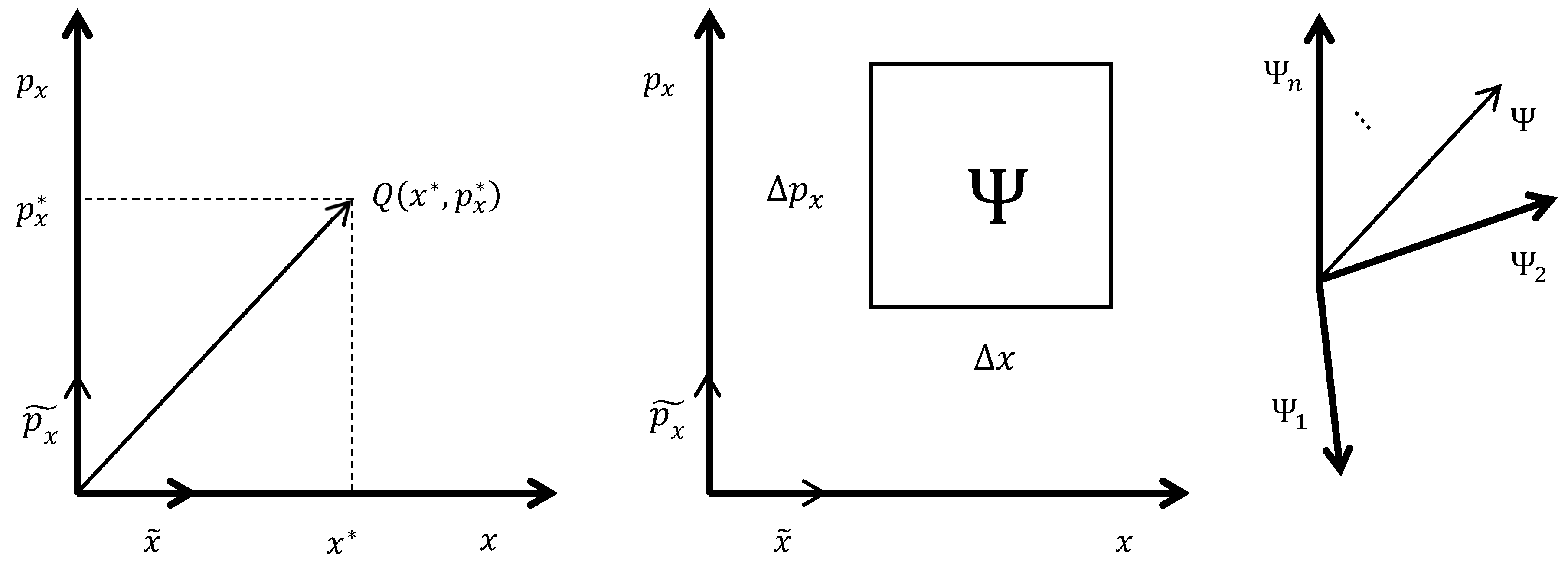
Figure 6.
(Left) position-momentum phase-space in CM for a single particle moving back-and-forth in one dimension with momentum . The phase-space is sectioned by a coordinate system (basis) with - and -axes. For particles in 3D, there are three dimensions of position and three of momentum per particle, for axes total in the basis. In 2D, we measure the value pair . That tells us the system occupies physical state . Ideally, when the uncertainties of both and are zero, the state is a point in phase-space. Each point is a different state of the system. Phase-spaces are linear vector spaces, so each point is also a vector (unique arrow from the Origin), like that to . The vectors and along the coordinate axes are perpendicular (orthogonal) to each other, linearly independent (li) from each other. For convenience, they are normalized (unit vectors; “~”), i.e., each divided by a constant to make its length equal 1. Linear combinations (sums of multiples) of and can generate any point in the 2D space. Any set of basis-vectors that can recreate the space that way is called a complete set or a basis. To span (recreate) the vector space, the number of basis-vectors must equal at least the dimension of the space and all basis-vectors must be li. When all basis-vectors are li and normalized, they form an orthonormal basis. (Center) the same phase-space for a QM particle. Now we cannot measure any variable pair exactly. Rather their uncertainties map-out a region in phase-space. The Uncertainty Principle specifies . Hence, the minimum area of the region is . One can draw similar boxes for and other non-commuting observable pairs. The quantum state occupied by the particle lives inside the box, a quantum world fundamentally invisible to humans and their instruments. (Right) all possible quantum states the particle could occupy are mapped out in a Hilbert space, the QM version of phase-space. Every quantum system has a Hilbert space. The dimension of a Hilbert space is the minimum number of li subspaces needed to span it, i.e., the size of its basis. It also equals the sum across species of the degrees-of-freedom (independent quantum states) per particle times the number of particles in the system. ranges 2-. (The figure shows a finite for illustrative purposes, but, in actuality, the Supermicroscope has .) The subspaces in a basis are typically rays, i.e., axes or 1D-subspaces, each spanned by a unit vector. Each subspace is a quantum state unto itself. Infinitely many different bases span a Hilbert space; one need merely pick another set of li axes for an equally valid alternative basis. Commonly, the basis chosen is one made-up of the eigenstates of whatever measurement variable (observable) is currently being measured. Any quantum state in the Hilbert space can be resolved into these eigenstates .
F. State Space
1. CM Phase-Space. How QM arises from the Uncertainty Principle is illustrated with an idea (Figure 6) of Planck’s (1916). To understand this, we first discuss CM phase-space, or state space. State spaces are much used in thermodynamics, Planck’s field. Every CM system has an abstract state space “floating alongside” the actual physical space occupied by the system. Figure 6 shows the state space for a single particle in the Supermicroscope of Figure 3. It has two axes (two dimensions) for the two degrees-of-freedom of the particle. One axis is for position (back-and-forth along a straight line); the other for momentum . For particles moving in 3D, instead of one particle in 1D, we would have three coordinate axes for the position and three for the momentum of each particle in the system. Hence, the state space would have axes. Further axes, e.g., if there are electromagnetic fields, are added as relevant. Going back to Figure 6, in the ideal CM case, both and can be measured exactly. Thus, at any time they specify a point in state space, the state , of the particle. If desired, one can reslice the space into different axes and express the state in terms of a new pair of variables, e.g., . Thereby, only the axes change, the point (the state itself) remains the same. For the physical information the state carries about the particle includes information not expressed explicitly, perhaps even unknown to the Observer. Each point represents a different state and the space is the collection of all possible states the system could occupy.
In linear algebra, the second major branch of mathematics used in QM, CM state space is a linear vector space. It consists of points and coordinate axes. One deep insight of linear algebra regards points: each point in a vector space is analogous to a vector is analogous to a function. It is easy to see that points are related to vectors. A vector is a directed line segment (arrow) from the Origin to the point in question, e.g., the vector to in Figure 6. Points and vectors are equivalent as there is one and only one vector to each (and every) point in a space. Indeed, one often denotes a vector by the coordinates of its point, e.g., . But how do points relate to functions? Well, point in Figure 6 is labelled explicitly as a function . Every point in the space could be labelled that way, its coordinates serving as the argument of the function. A unique state is assigned to each point like the one-to-one correspondence between points and values of a function. Readers may recall this idea from the elementary definition of a function : “ is a rule assigning to every point another point “. In QM and elsewhere one can, moreover, define vector spaces called function spaces, in which each vector is a function, like or , rather than an ordered row or column of numbers like . Thus, points, vectors, and functions in vector spaces are intimately connected.
A second deep insight of linear algebra is that coordinate systems are analogous to matrices are analogous to operators (transforms). A coordinate system or complete set of axes, also called a representation, is a way of mapping out a linear vector space. The Observer, especially in QM, has freedom in choosing a representation, with a couple restrictions we get into below. In choosing each axis, we assign a basis-vector rooted at the Origin and parallel to that axis. The axis itself is a ray, a 1D subspace of the vector space. (Vector spaces can also have 2D and higher-dimensional subspaces with multiple basis-vectors, but we touch on this only lightly.) Any point along a ray between 0 and may serve as basis-vector. But it is convenient to normalize each basis-vector, i.e., to multiply it by a constant that makes its length equal 1, in the units of the axis. The first restriction is that all the basis-vectors be mutually li, i.e., orthogonal. It means no one basis-vector is a linear combination (sum of non-zero multiples) of any or all of the others. The physical correlate of this restriction in CM is that each axis of the state space represent an independent measurement variable. E.g, no basis-vector should be simply a double or half of another, nor the simple sum of two other basis-vectors, etc. The second restriction is that the basis (the full complement of basis-vectors) span the space. I.e., by linear combinations of one to all basis-vectors it should be possible to generate every point in the space. Moreover, the basis should contain the minimum number of vectors needed to span the space. The physical correlate of this restriction is that a state space should accommodate any conceivable combination of measurement results that could come up in Nature (completeness) without a priori bias towards or against any of them (objectivity). If our basis is both orthogonal and normalized, we call it orthonormal. The vector pair in Figure 6 is an orthonormal basis. A complete set of basis-vectors clearly forms a coordinate system. These basis-vectors can also easily be arrayed one-by-one into the rows or columns of a matrix. So we see how matrices and coordinate systems are equivalent. Operators, like in , are functions-of-functions. Each function fed into yields a unique function . Matrices, like in , carry out operations or transformations on a vector when they left-multiply it, producing a unique vector . We’ve already said that vectors are equivalent to functions, so clearly a matrix is equivalent to a kind of function-of-functions, an operator. Transformations perfomed include such things as rescaling the length of , rotating it, inverting it, and more complicated effects. A further subtle insight underscores the equivalence of operators, matrices, and coordinate systems. From one point-of-view, a transform rescales, rotates, etc. a vector within a fixed coordinate system; but from an equally valid point-of-view, stays constant while the coordinate system itself is changed by the transformation. From the latter perspective, one can readily assent that a transform in a sense is a coordinate system. Especially when one contemplates the identity matrix
Identity Matrix (Transform)
The identity matrix, , which leaves every vector fully unchanged, is formally considered a transform unto itself. In QM, especially when working with function spaces, rather than as matrices, we often write operators as analytic expressions, for example, for the position operator or for the momentum operator in the -direction. (We will not go into how these expressions are derived.) Thus, coordinate systems, matrices, and operators in vector spaces are intimately connected.
Comment 9: One technical subtlety of vectors is important to philosophy. Above we said, if we transform to , the state does not change, only the axes. This is an intrinsic quality of vectors (and other tensors), they exist independently from the coordinate system in which they are expressed, and concomitant arbitrary human choices of scale and direction of axes. This independence is one reason for using tensors to denote physical quantities (forces, fields,…) in CM. The objective existence of these quantities free from human whim inheres in the vector space formalism. With the Theory of Relativity, Einstein believed he had attained the age-old philosophical goal of a truly objective model of Nature. This objectivity is implemented in the Theory in part through the tensor formalism. Inverted, this objective quality of tensors implies the existence of human freedom in choosing a set of axes arbitrarily to map out a linear vector space.
2. QM Hilbert Space. Returning to Planck’s idea, consider plotting the state of a quantum system, our particle under the Supermicroscope, on the phase-space of Figure 6. Even ideally in QM, and cannot both be measured exactly together. Instead, each has an uncertainty . Thus, rather than a point, they specify a region of area in state space at time . Per Eq. (5) the smallest possible area of this region is . Between measurements, the system quantum state dwells in this box unseen. Upon measurement, it manifests as any combination of values in the box of Figure 6. Per Planck, CM phase-space is insufficient for quantum systems.
In lieu of a CM phase-space, every QM system has a Hilbert space (Figure 6). Unlike CM state space, which is clearly abstract, it is debated whether Hilbert space is abstract or possesses some kind of reality. Like phase-space, Hilbert space is a linear vector space. It consists of vectors (points, functions) and coordinate axes (operators, matrices). Every quantum state the particle could possibly occupy is a vector in the Hilbert space and every vector in the Hilbert space is a quantum state. Thus, Hilbert space enables one to map quantum states as single points rather than as regions of phase-space. Like a CM state, a quantum state carries physical information about the particle, including information unknown to the Observer. But while a phase-state carries all the physical information about the particle in CM, whether this is true or not for a quantum state is again debated (Einstein’s hidden variables). Just as a CM transform, e.g., from in Figure 6 to , leaves a CM state unchanged, a transform from one representation to another leaves a QM state unchanged. For example, one of the probability distributions in Figure 4 was derived from quantum state expressed as a function of , , the momentum representation. The selfsame quantum state can be written as , the position representation. Each relevant observable for the quantum system, in fact, has its own representation. Each still harbors information about all observables. Thus, its Hilbert space accommodates every quantum state a quantum system could possibly occupy. Via the quantum state, the Hilbert space indicates the probability distribution for every variable that can be measured for the system.
Like phase-space, a Hilbert space is parcellated by coordinate systems (bases), matrices, or operators. Any vector in Hilbert space spans a ray, the line that runs thru it, a 1D subspace. (Alternatively, the vector, together with one or more others, can span a plane or higher-dimensional subspace.) Every point (every quantum state) along a ray can be converted into every other point by multiplying it by an appropriate constant. (The same applies if the Hilbert space is populated by functions rather than points. Then a ray consists of a set of functions that differ from each other only by multiplicative constants.) Thus, all quantum states in a ray are linearly dependent (ld) on each other. The usual choice to represent the ray as a basis-vector is the unit vector, created by dividing any non-zero vector in the ray by its own magnitude. Any set of li basis-vectors large enough to span the Hilbert space is a basis, a scheme for dividing the space into subspaces. The minimum number of basis-vectors needed is the dimension of the total Hilbert space (). The dimension derives from the particle species (quantum states per particle), the number of particles of each species, and the conditions imposed (e.g., any external fields) for the quantum system. Any basis chosen by the Observer is equally valid. But a very common and useful choice in QM is a basis formed by the eigenstates of whatever observable is curently being measured or discussed. In CM, a measurement variable, an observable is a single axis, a 1D coordinate system insufficient to span the space. A state is specified by the values of multiple observables, each along its own axis. But in QM, an observable is a multi-axis coordinate system. It is a basis for the Hilbert space, a way of dividing it up, a selective (and incomplete) perspective on it. Each axis thereby is a quantum state, in fact an eigenstate of the observable. For an observable is equivalent to a matrix or operator and matrices and operators have eigenstates and eigenvalues.
As we said, in QM Hilbert spaces are typically complex. How does one imagine that? The usual approach is to handle it as a pure mathematical abstraction. But here is one way you might visualize a complex Hilbert space (Figure 7). The key is to think of a regular rectangular coordinate system, a set of real axes. Each axis represents a different quantum state. But each real axis has its own extra imaginary axis sticking out orthogonal to it. Rather than, say, there being real axes for the quantum states in the basis of an -dimensional Hilbert space and one imaginary axis shared by all the real axes; no, there are real and imaginary axes. The phase of the individual quantum state is the angular displacement in the complex plane from its own real axis towards its own imaginary axis. Since, as discussed, the phase has no effect on the probability distribution of the individual quantum state, it is usual to draw the axes, if one draws them at all, at the zero-phase, i.e., pure real, position. Yet, the phase is significant when one sums quantum states, when quantum states evolve, etc.
G. Measurement, Observables and Other Operators
1. Effect of the Apparatus on the Outcome. In Figure 8, CM scenarios illustrate how an experimental apparatus sets the eigenvalues (possible outcomes) of a QM experiment. Flipping a coin is an everyday act, but also a very simple experiment. The coin is the sample, representing our quantum system. The coin has two different sides, like an electron with spin . This shows the contribution of the particle species to the possible outcomes. Were the obverse and the reverse of the coin identical, the number of possible outcomes would be halved. The apparatus might consist of the air and a tabletop. This represents the QM observable, the Hermitian operator. The tabletop forces the falling coin into the eigenstates heads (H) with eigenvalue or tails (T; ), where our outcome is the ccw angle the coin makes with the tabletop. The main point is, whatever angle the coin was landing at just before impacting the table, the flat tabletop forces it into eigenvalue or and into eigenstate H or T. The same experiment with a die has six equiprobable outcomes, underlining the fact that the system itself provides the primary probability distribution. As a further scenario, imagine our table has outer wings, slopes, and a plateau (Figure 8). Then we can measure heads-up states and tails-up states . Note that the outer wings enhance the probability of , by increasing their surface areas. This shows that the apparatus, in addition to setting eigenvalues, can also influence the distribution. Finally, if our apparatus consists of air and a blitz camera, we can capture infinitely many eigenstates of the system (the coin spinning in air) with eigenvalues .
Comment 10: In O’Neill & Schoth (2023) we introduced an algebra for fractal geometries. There is an analogy between measurement in fractals and QM measurement (including entanglement, Part III). The analogy extends to the extraction of meaning from a mental concept. In each area it involves superimposition of direction and/or scaling onto a system.
Figure 8 illustrates how an apparatus imposes a basis (coordinate frame) onto a QM system. The choice of observable fixes the range of answers to the question posed by the experiment. The allowable eigenstates are preferred coordinate axes and the corresponding eigenvalues are scalings along these axes. A different apparatus (different observable) allows a different set of eigenvalues and eigenvectors. A measurement brings the system state out of a random field of possible answers into a determined state.
Measurements undertaken on fractal systems work rather the same. A famous question (Mandelbrot 1967) in fractals is, “How long is the Coast of Britain?” The answer depends on the size of your ruler. If it is 20 km long, you get a certain value. If it is 10 km, you get a different, larger answer. If it is the size of a boulder, you get a much, much larger answer. If it is the size of a grain of sand, you get an enormously larger answer. And so on. Scale inheres neither in QM nor in fractal systems. Rather it is imposed from outside. The analogy continues in that both fractal and QM systems have internal structure. In QM, we have particle degrees-of-freedom, e.g., possible spin states; in fractals we have the fractal dimension and fixed ratios between segment lengths that hold for all scales. If fractal geometry is intrinsic to Nature (Mandelbrot 1982), then it is perhaps unsurprising that quantum systems, to be measured, require external imposition of scale from the apparatus. That the apparatus imposes scale on the quantum system it measures again reflects a holism of Nature, she does not reval her character in the absence of an apparatus and even then only as gauged by the apparatus.
In outr theory of higher brain functions (O’Neill & Schoth 2023), information similarly possesses internal structure, but is free of meaning. Consciousness must superpose a context onto information in order to extract meaning from it. Meaning is dependent on context similar to the length of a fractal structure depending on the size of the ruler or a QM eigenvalue depending on the choice of measurement variable. In our earlier work, thereby, “context” means applying multiple coordinate (attribute) axes, each with its own scale. Meaning is the answer obtained for the context applied. Further, it is the quantity that gets (or can be) exported for action (behavior). The contrast of the - vs. -representation in QM compares with the sentence vs. context representation of concepts in our theory. Such representation allows calibration of action using the scales of context, including past time context pulled up from memory. Thus, in higher brain functions, in fractals, and in QM, the measured value (eigenvalue) depends on the apparatus.
Comment 11: Smolin (2019) and many others have asked, what is special about measurement? Aren’t measuring devices and the people who use them ultimately made of QM particles that obey the Schrödinger Equation and other QM rules? Here is what is special about QM measurement: To conduct a measurement is to stake an epistemological position. In the Dual-Slit Experiment (Figure 2), for example, one assumes the two slits are perfectly parallel and perfectly perpendicular to the screen. The slit edges are perfectly sharp and infinitely high. All dimensions remain constant throughout the experiment. The screen registers every arriving electron without error. It is perfectly smooth with uniform properties across its surface. Etc. In reality none of these assumptions are true. There are tiny bumps on the screen, etc. Ultimately, one could pursue all such irregularities down to the quantum level. In actual design, however, they (including quantum effects within the measurement device) are rolled into the measurement error of the experiment. In principle, at least in the first design stage of a QM experiment, only the subject (the sample) is regarded as quantum; the parts of the measurement apparatus are treated as in CM. Moreover, in Feynman’s formulation of QM (Feynman & Hibbs 2010), the CM action plays as important a role as the QM action to which it is characteristically normed.
One might say CM instantiates a “Zen solution” to a philosophical problem of Classical Antiquity: Is the motion of a flying body pulled from outside or propelled from within? CM divides the responsibility. As seen in the definition of the Hamiltonian (Eq. (8)), the motion arises from the interplay of kinetic (; which includes inertia) and potential () energy. is assigned to a single point, the c.g. Except for unusual geometries, the c.g. lies inside the body, while , in principle, is assigned to the entire Universe. Unless our system is a galactic mega-cluster, that lies overwhelmingly outside the body. These are, of course, two absurdities. But together they work; CM functions “by virtue of the absurd”, perhaps in the sense of Kierkegaard (1843). CM elegantly sidesteps the either/or problem by rephrasing it as “both”. QM similarly offers a solution to the ancient problem of Determinism. The solution is again arrived at by division. On the one hand, CM objects always behave deterministically and the QM quantum state evolves deterministically between measurements. But QM objects behave indeterministically during measurements. That’s why measurement is special. CM presumes a future, QM lets the future happen.
How an Observer, an Experimenter, or an Analyst decides to cut-up the World into CM (apparatus) and QM (particle) pieces is an epistemological question. The ontological parts of the formalism are that the past-- deemed classical once defined for a given set of objects—is irreversible and the future – once a basis of possible outcome vectors is defined—is unpredictable. In having the courage of our convictions, i.e., in preserving rigor, in conceding the independence of nature from our arbitrary preferences, we become empowered to predict events (or at least their probabilities) quantitatively.
Again, to take a measurement is to stake an epistemological position. Weighing meat at the butcher’s shop, for example, one accepts the scale is properly calibrated. I.e., one picks a “0”, a “1”, and an “∞”. “0” or wherever the arrow points on the dial when the tray is empty is accepted as no meat at all; “1” is the finest hash mark on the dial, quantities below one-half of that are neglected by rounding; “∞” is the direction of greater weight, usually cw. There are further conventions, e.g., is the fat to be trimmed or left on before weighing? One accepts the spring is Hookean, i.e., within a practical range, its elasticity does not vary with the load. Hence, even the simplest measurement entails a plethora of assumptions.
The Laws of Physics are typically applied to idealized objects. These include Hookean springs, frictionless pulleys, perfectly rigid bodies, non-buoyant air, etc. Even when not neglecting air friction, one graduates into Hydrodynamics with its potential flows, incompressible fluids, Newtonian fluids, etc. At each level, certain approximations come into play to allow the calculus machinery in which the Laws are written to operate. This is quite the same as in classical logic. To complete a syllogism, for example, “All men are mortal, Socrates is a man, therefore, Socrates is mortal,” one must accept the premise. Thereby, one is staking an epistemological claim that then allows the machinery of formal logic to work. Here one is reminded of Einstein’s (1921) famous quote, “Insofern sich die Sätze der Mathematik auf die Wirklichkeit beziehen, sind sie nicht sicher, und insofern sie sicher sind, beziehen sie sich nicht auf die Wirklichkeit.” ( “As far as the laws of mathematics refer to reality, they are not certain; and as far as they are certain, they do not refer to reality.”) In physical modelling, one pursues reality thru successive, unrealistic but effective approximations.
2. Projection Operators. Observables correspond to coordinate systems, matrices, or operators in Hilbert space. As stated, each eigenstate of an observable is a quantum state in its own right. The eigenstates together form a basis for the Hilbert space. Any set of li quantum states serves as a basis spanning an -dimensional Hilbert space. Any quantum state in the space can be resolved into any basis
Resolution of Quantum State Into Basis
The terms are the components of , its vector projections onto each subspace. are the projection operators or projectors of the basis. We have chosen an orthonormal basis, therefore, the coordinates (expansion coefficients) satisfy . As mentioned, it is common and useful to resolve into a basis formed by the eigenstates of an observable. The eigenvectors (or higher-dimensional eigenspaces) of the operator representing each observable must form a basis that spans the Hilbert space of the quantum system. A proper QM observable must be a complete set, it must contain enough independent dimensions to specify every point in the Hilbert space. This is a criterion for a well-composed quantum experiment. Thus, if we think of quantum states as vectors in Hilbert space, we can think of QM operators as coordinate systems in the same Hilbert space. Similar to transforming from to in CM, in QM one can transform the basis of from one observable to another. Thereby, the quantum state itself, being a vector, remains unchanged. A deep assumption of QM is that the state, representing physical information about the system, can always be resolved into the independent eigenstates of a measurement variable. This is Feynman et al.’s (1964) Great Law of QM, expressed by Eq. (13).
Each observable in QM is an operator, a set of orthonormal eigenvectors that spans the Hilbert space in a different way. Moreover, the observable itself can be expressed as a sum of its projectors onto each of its eigenspaces, weighted by the corresponding eigenvalue
Spectral Decomposition of QM Operator
where
QM Projection Operator
is the projector onto eigenspace . Interestingly, the coefficients of each term in Eq. (14) are the respective eigenvalues whether the corresponding eigenspace is a 1D eigenvector or a higher-dimensional eigenspace. (In this sense, eigenvalues are more general than eigenvectors.) In understanding Eqs. (14-15), it is useful to notice that and , being orthonormal basis vectors of , have 0 for all components except , which is 1. The expression is a dyadic product creating a matrix, here
Just as Eq. (13) says a vector can be resolved into a sum of component vectors, Eq. (14) says an observable can be decomposed into a sum of matrices. The latter represent each of the subspaces that sum together to create the overall space. Is thus one scheme for parcelling-up the Hilbert space. The eigenvalues are the weightings, telling how much each eigenspace contributes to the observable (i.e., contains some fraction or multiple of each subspace, not necessarily equal 1). The measurement of each variable, chosen by the Observer in Process 2, is a different perspective on the quantum system.
Upon measurement, the system shifts into a quantum state that is one of the eigenstates of the observable being measured-- chosen at random-- and the system expresses itself in the macroscopic world solely in the form of the eigenvalue of that eigenstate. The ensemble of eigenstates of the observable forms an alternative set of axes, an operator, spanning the Hilbert space. The eigenvalues represent a kind of scaling, the contribution of each eigenstate to the measurement operator. Here is one way to grasp the QM law whereby a quantum system always shifts into an eigenstate of the observable operator immediately post-measurement. It is simply a more general, more systematic way of expressing the inevitable but unpredictable effect of the experimental design on the measured outcome that we saw in our Heisenberg Supermicroscope.
The probability of measuring eigenvalue is
Probability of Measurement Outcome (pure state)
After this outcome, the system assumes the corresponding quantum state
Post-Measurement Outcome (pure state)
The expectation value is
Expectation Value (pure state)
There is, however, an exception to the unpredictability of the post-measurement state. If the particle is already in an eigenstate of the observable at time of measurement, the value measured in the experiment will always be the eigenvalue of that observable, no matter how many times the measurement is repeated. And the system will remain in that eigenstate, no matter how many times the measurement is repeated. This occurs because projects onto itself and because for all projection operators and any positive integer , a property called idempotence. This is one QM version of reproducibility. It ties QM to empiricism. (The other version is the above-mentioned reproducibility of QM distributions.)
Comment 12: Smolin (2019) has pointed out an important distinction between quantum states before and after measurement. While the input state is a superposition of states with definite values of some observable, the output state corresponds to just one value. Note that Halvorson (2012) has emphasized that the output state, too, can be resolved into a linear combination of multiple other states, although these states must form some other basis that spans the Hilbert space.
2. Operators: Position and Momentum Representation. Operators can be formulated in terms of any measurement variable. Two common choices are expression in spatial coordinates, e.g., , (position representation) or in momentum coordinates, e.g., , (momentum representation). (Figure 4, for example, uses momentum representation.) As seen above, and themselves, as well as their components and , are measurement variables and therefore have operators. In position representation, the 3D position operator and its component operators are . Each operator is smply the function itself. Easy. But in momentum representation they are more complicated , respectively, . In momentum representation, the 3D momentum operator with component operators . Again easy. In position representation they are , and . In cases where kinetic energy is purely translational (not rotational or electromagnetic), its operator is in position representation and in momentum representation. For potential energy we have in positiion and in momentum representation. The exact functional form of depends on the experimental paradigm; in fact, appropriate formulation of is a common way of incorporating BCs into a QM problem. With the above expressions, we can write a version of the Schrödinger Equation in position representation
Time-Dependent Schrödinger Equation (no rotation, EM field)
widely encountered when there are no electromagnetic fields or rotation.
The exact form of in Eqs. (7,20) depends on the scenario and is one way, along with the BCs and ICs, the experimental set-up influences . The particle species influences , among other ways, through its mass and its charge (if there are electromagnetic fields). Hence, Eq. (20) tells us that and, ultimately, the probability distribution for measurement outcomes are jointly affected by particle-intrinsic and external factors. Additionally, the total energy of the quantum system determines how rapidly the probability distribution evolves in time. As QM commentators are fond of remarking, this evolution is itself deterministic (i.e., laid down by Eq. (7)) while experimental outcomes are randomly picked-out of the distribution at time of measurement.
3. Steady-State Schrödinger Equation. For a particle of definite energy, i.e., a quantum system of constant energy , Eq. (7) reduces to
Time-Independent (Steady-State) Schrödinger Equation
the Time-Independent or Steady-State Schrödinger Equation. This is the equation used, among many other applications, to calculate atomic and molecular orbitals of stable atoms and molecules. Famously, it is an eigenvalue equation, as is the equation for computing the eigenstates and eigenvalues accessible to any measurement variable. Each solution to Eq. (21) is a physically allowable quantum state (eigenstate) with corresponding energy level (eigenvalue) for the stable system.
4. Heisenberg Picture: Unitary Evolution. Eq. (7) is written under the so-called Schrödinger picture of QM. In the Schrödinger picture, evolves in time under the actions of the Hamiltonian, which itself is frequently time-independent . In an alternative formulation of the Time-Dependent Schrödinger Equation
Time-Dependent Schrödinger Equation (Heisenberg Picture)
under the Heisenberg picture, the quantum state itself is not an explicit function of time. It is instead taken at some fixed time . The time-variation is rather built-into a time-evolution operator . acts on to yield the quantum state at an arbitrary new time . The Heisenberg and the Schrödinger pictures are equally valid formulations of QM. The choice between them is one of convenience. In O’Neill & Schoth (2022) we cited the twin notions: “Time is the one thing that changes when everything else remains the same” (Schrödinger picture) or “when nothing changes there is no advance in time” (Heisenberg Picture). QM preserves the philosophical ambiguity in these alternative quantitative pictures.
The time-evolution operator is a unitary operator, an operator whose adjoint equals its inverse . Hence, except in the special case , is not an Hermitian operator (). Therefore, is not itself an observable. is called “unitary” because it does not change the magnitude or length of any vector or function it works on (it merely multiplies them by 1).
can rotate its argument in the complex plane. In the case of a particle of definite energy, the evolution of the quantum state is On the complex plane, this means causes the quantum state to rotate ccw about the Origin in a circle of constant radius . At each timepoint the quantum state is at angle with respect to the real axis. Since is periodic, each angle is revisited every . Thus, one thing QM tells us is that an isolated particle of definite energy will not change the magnitude of its quantum state spontaneously, no matter how long it is left to its own devices. It never jumps out of its fixed cycle of rotation. Length changes result only from external interventions, like measurements or superpositions (summations) with other quantum states. Moreover, the probability of observing the particle is not affected by its phase (angle on the complex plane). For, . Finally, QM texts often fail to mention that each quantum state in a system can rotate at its own frequency. In particular, we know from Eq. (3) . Thence, in a multi-state isolated system, one state can rotate as , another as , etc. The energy is the driver of the complex rotation.
Above, we multiply invoked the unitary operator for time translation (time evolution). Formally it is
Time-Evolution Unitary Operator
Further unitary operators of QM are:
Spatial-Translation Unitary Operator
Angular-Rotation Unitary Operator
Velocity-Boost Unitary Operator
is the quantum state evolves into when translated by time , the state becomes when translated by distance , the state becomes when rotated by angle about the -axis, and the state becomes when the velocity of all its particles is increased (“boosted”) by in the direction. (All these in the absence of other induced changes.)
Notice that each expression in Eqs. (23-26) involves a pair of non-commuting variables, i.e., a pair that obeys the Heisenberg Principle (see below). Thereby, one variable is expressed as an Hermitian operator, the other (except for parameter ) as the eigenvalue of an Hermitian operator. Hence, unitarity and uncertainty are connected. Each of Eqs. (23-25) is also associated with its own Conservation Law. Even in CM, Conservation of Energy derives from the concept that the results of an experiment are independent of a shift in time. (It makes no difference if we conduct an experiment on Thursday or Friday.) Conservation of Linear Momentum derives from the concept that the results of an experiment are independent of a shift in space. (It makes no difference if we conduct an experiment on the left or right end of the lab bench.) Conservation of Angular Momentum derives from the concept that the results of an experiment are independent of a shift in angle. (It makes no difference if the lab bench is parallel or perpendicular to the lab wall.) Eq. (26) is not associated with a Conservation Law per se, rather with an equally important principle from Galilean and Special Relativity. The results of an experiment are independent of the velocity of its frame-of-reference, as long as there is no acceleration during the experiment. (It makes no difference if an experiment is run atop the Rock of Gibraltar or on the deck of a cruise ship making 20 knots.) Moreover, each Conservation Law is linked, via the celebrated Noether’s Theorem, to a symmetry property of the system. Recall that none of these unitary operators changes the modulus of a quantum state; all they do is rotate it about the complex plane. In QM, Conservation Laws are thus expressed thru the independence of measurement outcomes from the phase of the quantum state, thru the equivalence of quantum states at different angles around the complex plane.
Comment 13: In QM observables are Hermitian operators. Hermitian operators always have real eigenvalues. Eigenvalues are the measurement outcomes. Experimental values manifest once in time. I.e., they do not rotate about the complex plane; they have zero imaginary component. Perhaps that is why measurement outcomes join the past, because they have ceased to vary in time. Eigenvalues are sometimes called “invariants” of the matrices or operators they represent. Measured eigenvalues are stripped down from the time-variance of their operators. Measurement is eigenvalue extraction that removes the active influence of time and therefore relegates the eigenvalue to the past.
Comment 14: Unitary operators for time and Hermitian operators for measurement outcome variables are clearly different. Yet, one wonders if time can also be a measurement outcome of sorts. In particular, is time the measurement of no intervention? In QM does such a time measurement take place purely external to the system yet represent processes occurring internal to the system? Is this possible because time has purely number character? I.e., number is a universal symbol fully free of attributes (O’Neill & Schoth 2022). It can thus reflect the objective because it is a “least common denominator” for information. It is simple enough to be shared as a convention between almost all people. The universality of number would thus imply the objectivity of time which makes it apt for tracking QM time-evolution.
5. Commutator. As an operator is a “function of functions”, a commutator is an “operator of operators”. The commutator of two operators is defined as
Commutator of Two QM Operators
If , and are said to commute; if , and are non-commuting. The commutator enables a general formulation of the Uncertainty Principle
Generalized Uncertainty Relation
Setting and into Eq. (28) yields (eventually) the familiar ; likewise for and . But if , and the Uncertainty Principle is clearly violated. Thus, non-commuting operator pairs obey the Heisenberg Relation; commuting pairs do not.
6. Pure States and Mixed States. At this point we note there are two main kinds of quantum states: pure states and mixed states. This paper deals mainly with pure states. They are easier to work with. But be aware that in practice mixed states are far more common (Klyshko 1995). For a single particle, a pure state is one for which we have maximum possible information about the particle. We know the exact quantum state it is in. “Maximum” means all information permitted by the Heisenberg Principle. We know the state because we have prepared the particle carefully. Maybe we derived it from a well-defined source, like decaying radioactivity. We sent it thru slits and filters. We deflected it with electromagnetic fields, etc. Or we know the state because we have just measured a property of the particle. As said above, the act of measuring shifts the system into the quantum eigenstate of the eigenvalue we just measured. If our system has multiple particles (or for repeated measurements on one particle), a pure state means the state is known and all particles are in the same state. The key point is, even if we have a single particle in a known pure state, we still have quantum randomness, there are still multiple different values the state can show upon measurement, all the eigenvalues of the observable being measured. As shown in Figure 4, controls the probability distribution of seeing the different eigenvalues, but no one can say for sure which value will pop-up in a given run. In a mixed state we have (a little or a lot) less than maximum information about the state. For a single-particle system, the particle can occupy any number of different states and we don’t know which one it is in. For a multiple-particle system, the various particles can be in different states and we don’t know which particle is in which. A common scenario for mixed states in QM, however, is that we know we have different states and the fraction of particles in state (or the probability of one particle being in ) is known to be . So, on top of quantum randomness, in a mixed state we also have randomness due to everyday lack of knowledge. This is the same lack of knowledge encountered in Classical Thermodynamics that underlies the entropy concept. Fortunately, and by great ingenuity of its founders, the formalism of QM can handle this scenario rigorously using the density matrix or density operator . For a mixed state, essentially takes the place of in the various equations of QM.
For projectors defined as in Eq. (15), the density operator is
QM Density Operator
The time-evolution of a mixed-state is given by
Liouville-von Neumann Equation (Schrödinger Picture)
Liouville-von Neumann Equation (Heisenberg Picture)
the differential, respectively, matrix forms of the Liouville-von Neumann Equation, which represent the Time-Dependent Schrödinger Equation (Eq. (7)) for the density operator. The probability of obtaining eigenvalue after measuring variable is
Probability of Measurement Outcome (mixed state)
After this outcome, the system assumes the corresponding quantum state
Post-Measurement Outcome (mixed state)
The expectation value is
Expectation Value (mixed state)
The QM entropy is defined thru the density function
von Neumann Entropy
This von Neumann Entropy is essentially the celebrated Shannon Entropy (Shannon 1948) of the mixed state
Shannon Entropy
only expressed as the natural logarithm rather than log2 and multiplied by the Boltzmann constant . The von Neumann Entropy is the connection between QM phenomena and macroscopic thermodynamics, such as we explored in O’Neill & Schoth (2022). Together with the internal energy
Quantum Statistical Mechanical Internal Energy
which is set equal to the Hamilton operator, the entire edifice of Quantum Statistical Thermodynamics can be derived from the von Neumann Entropy.
In particular, the thermodynamic volume operator serves as a control parameter (argument) of , . The thermodynamic pressure operator is
Quantum Statistical Mechanical Pressure
and the thermodynamic temperature operator is
Quantum Statistical Mechanical Temperature
Further expressions can be derived for all classical thermodynamic variables.
Comment 15: Smolin (2019) has also remarked that what is powerful about the Shannon entropy is that it measures how much information a message transmitted independent from what the message means. Sender and receiver share a semantics (code) that gives meaning to the message, but even one who doesn’t know the code can measure the quantity of information carried. This is similar to Saussure’s signifiant-signifié distinction (de Saussure 1916), in which the arbitrariness or historical conventional character of the symbol used is emphasized. It is in opposition to McLuhan’s (1964) popular “the medium is the message” dictum.
7. Wavefunction. As mentioned, an observable can have infinitely many eigenvalues and eigenstates. These eigenvalues and eigenstates are frequently continuously distributed in QM. For example, the operator for the 1D-position observable is simply itself. (The eigenstates are a continuous string of Dirac delta functions , one for each -value.) In the case of the free particle, a particle flying around by itself in empty space unmolested, for example, the particle may be observed at any value in the continuous range . In such cases, it is useful to replace a set of discrete quantum states with a continuous wavefunction . Rather than a probability amplitude, is a probability density function. Specifically,
1D Position Wavefunction Normalization
The integral of the modulus of the wavefunction across all possible position values is unity, the sum of all probabilities. Choosing such that Eq. (40) equals unity is a further instance of normalization. Physically, normalization means the particle will, with certainty, exist at some point along the -axis. If it is to be a “real” particle, it must exist somewhere in space. is thus probability per unit length, linear probability density. itself (and ) have units of . Along the same lines, we have
2D Position Wavefunction Normalization
and
3D Position Wavefunction Normalization
In these cases, , respectively, and represents probability surface density, respectively, probability volume density.
Upon conducting any measurement on the particle, the infamous “collapse of the quantum state” occurs. The particle is shifted into just one of the constituent eigenstates. The corresponding eigenvalue is the actual measured value of the variable. As such, the eigenvalue is the real-world expression of the particle. Thus, measurement is another way for quantum particles to join the macroscopic world. The eigenstates correspond to points where the observable is uniquely defined, i.e., where the value is measured with certainty. These are points of for measuring the eigenvalue. If measurement is repeated when the quantum system is in one of these eigenstates, it always returns the corresponding eigenvalue . The fact that such points exist, links the wavefunction to the empirical world.
Comment 16: Further remarks on collapse of the quantum state. QM measurement is irreversible in the sense of the Second Law of Thermodynamics, the Arrow of Time. Whatever their probabilities beforehand, once a measurement is made, all eigenvalues, except the one observed, assume . The observed eigenvalue jumps to . This means the event of observation “joins the objective past”. Each eigenvalue is distinct, hence observing one is something like registering an idiosyncrasy. For every event in the past is unique and we enumerate them as such. Every day, for example, someone different is born and someone different dies. The evolution of the quantum state can run forward or backward in time, but the collapse runs only forward. Hence, quantum events continuously create a record of the past as they plunge thru the present. Since every quantum system has at least two eigenstates and it is not fixed which will be observed, the future in QM remains intrinsically open, albeit within a system-specific range of possibilities. As QM events lay down history, they build physical context, including the macroscopic constraints, BCs and ICs, etc. that impact the form of the Schrödinger Equations from which quantum states are derived. This would be one mechanism by which quantum behavior is influenced by holistic factors.
The collapse of the quantum state leads to a change of state of a CM object, e.g., a pointer on an instrument moves from “0.0” to “0.2”. The CM state is objective in that it is the same for all Observers sharing a “least common denominator”, i.e., a common lower limit on precision. The physical content of QM is that, at the finest levels, the limit is universal. Just as is a universal limit on the rate of information or energy tramsfer in Special Relativity. While is a limit on how fast we can go, is a limit on how much we can know. This may be one way of unifying Relativity and QM: The collapse of the quantum state is the transition between the realm of and the realm of . Peres (1995) points out that there is nothing mysterious about quantum jumps, the collapse of the quantum state. What is jumping is not the quantum system itself, but rather our arbitrary description of the apparatus. Before the measurement, it is sensitive to QM effects, after, it is treated as a CM object. CM language is also what distinguishes the past from the future, even if the dynamic laws of physics are basically time-symmetric. In going from the QM microstate of the particle to the CM macrostate of the observation, one is invoking an approximation, e.g., the approximation that the collapse takes place instantaneously.
A probability amplitude is apt for describing something that now exists, now does not. I.e., something on the edge of being. Once measured, a thing exists, it belongs to the physical realm of the measurable. The collapse of the quantum state means that some entity must have manifested, must have appeared at some point in space-time. Otherwise it would not belong to the physical realm at all. Before the measurement, the entity is unbound to any place or time because it belongs to the aphysical (unmeasurable) realm. Therefore, a particle is permitted to be in two places at the same time, i.e., it has a certain probability of being here and a certain probability of being there. The von Neumann formalism of QM measurement (Clifton 1995) expresses a state-of-mind, whereby from our macroscopic perspective, we insist that the measurement occur at a fixed point in time and the observable may have only one value at that time. The Measurement problem of QM arises because we examine the microscopic world with a macroscopic lens. Naturally, the image we get is distorted.
When a QM measurement is complete a “concept” is born. I.e., a “category exemplar” is born. E.g., following one trial of a QM experiment, a pointer indicates “1.1”, selecting one possible QM outcome of a set. After a second trial, the pointer shows “1.2”, indicating a second possible outcome in the set. Etc. The outcome “1.1” is a macroscopic entity, the pointer pointing there is a macroscopic event. It exists at the macroscopic level of approximation, like a thermodynamic macrostate. Thus, the attainment of a QM outcome is an irreversible event. Language is based on concepts, it is structured in concepts. Behavior is similarly structured in concepts. Observers in community can come to an accord on concepts.
Comment 17: A further factor supporting the ontological nature of the quantum state is that it acts as a vector in Hilbert space. The definition of a vector in linear algebra includes the notion that the vector exists independently of the coordinate system in which its coordinates are expressed. For this reason, vectors have won favor in CM for describing physical quantities like forces, electric fields, etc. that exist objectively and independently from our human choices in measuring them. That quantum states are so well modelled by vectors suggests that they, too, have objective physical character.
Comment 18: There has been much debate about the quantum state or its close cousin, the wavefunction. Is it a bona fide physical entity or a pure mathematical construct? Alter & Yamamoto (1995), for example, consider the observables in QM to be aphysical as they are subjective, defined by the artificial and arbitrary whim of the Observer in constructing the apparatus. They regard the quantum state to be the truly physical entity as it is objective, i.e., its random behavior is independent of any Observer. Many take the opposite tack: what is physical is what is observable, the measurement variables or at least their eigenvalues; quantum states are aphysical idealistic abstractions since they cannot be observed. Hence, one reason the debate around the quantum state has been so enduring may be that it pits Objectivity vs. Empiricism. Most hard-headed people would like to retain both, but QM demands they sacrifice one. We suggest the quantum state is an “ontologico-epistemological hybrid”. As philosophers know, ontology deals with what can and cannot exist; epistemology with what can and cannot be known. Simply writing a wave function we see real physical variables in the argument of and a real physical unit, “m” (albeit to a fractional power) in its denominator. As mentioned, a normalization condition on a quantum state also grounds it in physical reality. These are the ontological parts of . , meanwhile, stores information, a low-grade form of knowledge, about the particle. Its numerator is a unitless probability amplitude telling us the limits of what can be known about the particle. These are clearly epistemological features. Hence, is an ontological-epistemological hybrid.
Empiricism is about predicting and accounting for historical observations. These observations are made macroscopically with CM and all the assumptions that pertain thereto. Thus, von Neumann definiteness (Clifton 1995) and the collapse of the wavefunction are built into QM to keep it empirical. I.e., to keep QM responsive to the enormous mass of existing, to be made, and hypothetical CM measurements it underlies.
In QM, the future is open. I.e., within the experimentally prescribed state space, something novel and non-deterministic is permitted to arise. If something new can arise, that implies that it didn’t exist beforehand. Therefore, QM bridges the gap between existence and non-existence. The formalism of as an ontological-epistemological hybrid is apt for describing something that now exists physically, now not. Alternatively, one can widen the definition of physical reality to include such ephemera.
Comment 19: Frye (1992) draws a deep distinction between knowledge and wisdom. Knowledge he relates to the past, to facts about and interconnections of what did happen. Wisdom, in contrast, relates to the future, to probability distributions of what could happen. Human experience and expertise consist, to a degree, in effectively managing probabilities. Especially in learning the less likely outcomes, when they should be heeded, and when they safely can be neglected. QM informs us that the World is intrinsically and inescapably unpredictable. Therefore, there will never be an “End of Wisdom”. There will always be a place for reasoned and seasoned judgement, even in technical affairs.
Comment 20: A probability amplitude describes something that now exists, now does not, i.e., something on the edge of existence. But once measured, the thing exists, i.e., belongs to the physical realm, the domain of the measurable. The collapse of the wavefunction means the entity is compelled to manifest, i.e., it must appear at some point in space at some instant in time. If not, it would not pertain to the physical world. Before measurement, the entity is not bound in space-time, for it is part of the immaterial (non-measurable) world. Therefore, a QM particle is allowed to be here and there at the same time, i.e., it has a certain probability of being here and a certain other probability of being there. Normalization implies that, if the particle is to be part of reality, it should become upon measurement, it has to show-up somewhere in the Universe. The non-locality of QM expresses the fact that the site of appearance upon measurement is not deterministically fixed a priori and that there is no exact position set between measurements.
Comment 21: It is rarely well explained why not just the eigenstates of an observable but also all their linear combinations validly represent the state of a quantum system for a given scenario. On one level, this is the surely the case because quantum states are solutions to the Schrödinger Equation. The Schrödinger Equation is a (partial) differential equation and all linear combinations of solutions to a differential equation are themselves also solutions. For more intuitive understanding, think back to Figure 3. We measured position and momentum of the particle using the hash marks on the graticule of the supermicroscope. The distance was constant between each pair of hash marks, but the value of the distance was arbitrarily chosen. We could have as easily used hash marks twice or half as far apart. Allowing arbitrary multiples of the quantum state to represent the particle permits particle behavior to be independent of this arbitrarily choice. When one has more than one dimension, we have arbitrary scalings along each axis and arbitrary orientation of the axes to contend with. Allowing all linear combinations of the basis quantum states to represent the particle keeps its behavior independent from all these subjective experimental choices.
III. Entanglement
Quantum entanglement is a much talked about and controversial theme in QM that is challenging to grasp. Below we try to render this topic concretely and mathematically understandable. We explain how, in its essence, entanglement reduces to the concept of correlation. We discuss the (in)famous idea of “spooky action at a distance”, which some consider a bug, others a feature of QM. We touch on similarities between measurement and entanglement in QM. Finally, we discuss the relationship of entanglement to macroscopic objects.
A. Simplified Mathematical Formalism of Entanglement
1. Composite Quantum States in Hilbert Space. Two or more particles can form a composite quantum system. The Hilbert space of a composite system is generated by taking the tensor product (denoted ) of the vector bases of its isolated particles.
Let us take the usual example of a system composed of two particles A and B. The basis of A is , that of B is . The basis of the composite system AB is, therefore
Basis of Two-Particle Composite QM System
That means that AB, in principle, can occupy any quantum state of the form
i.e., any state that is an LC () of the four new basis-vectors.
Among the quantum states in the composite Hilbert space are all combinations of the states of the isolated constituent particles. These are also formed using the tensor product. Suppose, for example, we have the state for isolated particle A and the state for isolated particle B. This pair corresponds to the state in the composite Hilbert space. We write this
2. Separable and Entangled States of a Quantum System. Once a composite system is constructed, however, it is not restricted to states of the form (44). The system is permitted to occupy any state of the form (43). On the one hand, this includes states of form (44), for which for every term in Eqn. (43), i.e., for every component of the composite state vector. These are called separable states. On the other hand, the system can also occupy states where for one or more components. Those are called entangled states.
A classic example of an entangled state is the state
An Entangled State of a Two-Particle Quantum System
is a perfectly legal state in the composite Hilbert space. We will now show, however, that there is no way to construct this state thru any LC of and .
To see this, first note that such an LC must have . Okay. But, simultaneously, we must have . Now implies either , in which case, , or , in which case, . Each contradicts a prior condition. Moreover, implies either , in which case , or , in which case . Double contradictions! Therefore, for any set of coefficients . One says that the entangled state cannot be factorized into the isolated states . Thereby, the concept “to factorize” concerns the tensor product and the coefficient pairs that it produces. If you can express a composite quantum state as , where is a LC exclusively of the basis-vectors of A and is a LC exclusively of the basis-vectors of B, then can be factorized and is separable; otherwise, is entangled.
Above, we said that, for mixed states, the number of quantum states a system could be in is multiplied due to lack of information on the true state the system is in. The quantum entropy is even formally derived from this lack of information. For composite systems, there is similarly a multiplication of the number of possible states the system can occupy. The entangled states are added to the separable states. This can be thought of as a kind of “entropy of mixing”. Indeed, the same mathematical formalism involving the tensor product is used for mixed and composite states.
3. Geometric Concept of Entanglement. Geometrically, one can imagine the Hilbert space of a composite system as divided into regions. Some regions consist of separable states, some of entangled states. A critical insight emerges when sharp constraints are laid upon the composite system. E.g., certain constants of motion may attend the system. While, as explained above, forming a composite system generally expands the range of available quantum states, sharp constraints can again restrict the set of permitted states to a subspace of the composite Hilbert space. When the system has a constant of motion, only states that respect its corresponding conservation law (Conservation of Energy, of Linear Momentum,…) are allowed. Fixed conditions can, moreover, restrict the choice to certain entangled states or to exclusively entangled states.
4. Entanglement and Correlation. In its essence, QM entanglement can be seen as correlation. Let us explain. Imagine again a composite system AB consisting of particles A and B. As we said above, the basis-states will be available to AB. As noted, these are paired combinations of the basis-states of the isolated systems A and B. Now an Observer, of course, can perform measurements on A or B whether they are isolated or belong to the composite system AB. In the latter case, we ask, to what extent does a single measurement performed on A influence a subsequent (or preceding) single measurement on B? The correlation coefficient expresses this influence quantitatively. tells us, how often eigenstate of B accompanies eigenstate of A. Or, what means the same thing, how often measurement value (eigenvalue) of B arises, given eigenvalue of A.
In brief, the degree of influence ranges from zero to completely determinant. If AB is in a separable state, . The measured value of B is fully independent from that of A. For any value , however, we have entangled states. means that the appearance of promotes the appearance of ; (anti-correlation) means the appearance of hinders the appearance of . The words “promote” und “hinder”, thereby, are to be understood statistically.
5. Spooky Action at a Distance. The most famous (and controversial) example of QM correlation is a two-particle system AB as described above. A and B are created together at the same point in space-time, e.g., through fission of a mother particle D. Immediately upon creation, A and B fly rapidly apart in opposite directions in a straight line across space. They encounter no other particles or external fields along the way. D originally had total spin angular momentum . If A and B are fermions, on account of Conservation of Angular Momentum, we must have (It’s customary to pick and AB an electron or electron-positron pair.) The total spin angular momentum of AB is a constant of the motion. That is the case at the point of origin and at all later times, no matter how far apart the particles are. Alternatively, A and B can be bosons. Then the particles maintain regardless of distance apart. (Customarily, one chooses , a photon pair.) The condition that angular momentum be conserved restricts the set of permitted states to a subspace of the Hilbert space of AB within which ; it entangles A and B. The set of AB-states in Eq. (44) is no longer available. Instead, the system occupies states per Eq. (43), that look more like Eq. (45).
The most controversial aspect of entanglement has to do with measurement. If one performs a measurement on A, not only does the measurement set the QM state of A, but of all the constituent particles, of the total composite system AB. And that happens immediately, no matter how far apart the particles are. A and B could be meters apart, or kilometers. They could even be so far apart, that a signal travelling at would be incapable of breaching the distance between A and B before A and B flip their QM state on account of the measurement! That is an apparent violation of Special Relativity Theory (SRT), which limits the maximum rate of information transfer in the Universe to . Einstein famously called this effect “spooky action at a distance”. It is an extreme example of the also characteristically quantum mechanical “collapse of the wave function”, which also occurs instantaneously. That is one reason, why Schrödinger (1935) claimed that entanglement contains all that is properly QM.
Many workers only experience this effect as spooky when particles A and B are separated by great distances. Although they are just as entangled with one another, hardly anyone is bothered by the coupling of the measured spin values of the paired electrons in the 1s-shell of an atom. But in principle, this coupling is just as much (or just as little) a violation of SRT. Be the particles divided by Ångströms or kilometers, the measurement effect apparently traverses a physical distance with unrestricted speed, faster than light even. We will see presently, however, that there is actually no violation of SRT. But for the moment we merely remark that this QM-immediacy is the same as the immediacy of logic. Wittgenstein noted how we feel a sense of “flow” when we conduct a logical derivation. The mind flows step-by-step forwards until it finally lands at a proof, e.g., of the Pythagorean Theorem. But, according to one major view of mathematical truth, the Pythagorean Theorem was true long before the dawn of mankind and will still be true long after our extinction. According to Wittgenstein therefore, the theorems and axioms of logic are less like the spurts and eddies of an ephemeral rolling stream and more like the fixed members of a work of eternal architecture. Similarly in QM, the measured spin values of particles A and B are always opposed because the Conservation of Angular Momentum never ceases to apply. Important to note: the two exact measurement values for A and B are not fixed, rather their sum is. This sum is conserved at all times, but the individual values are allowed to differ. Outside the context of measurement the individual values are undetermined. Sometimes A has spin and sometimes . QM includes Determinism, but it is a Determinism of the overall entangled system, not of its single particles.
In the case of a separated state of AB, one notes no coupling of eigenvalues. Suppose we perform a measurement on A alone. The entire system, i.e., B included, shifts immediately into an eigenstate of AB. One possible state of A and one possible state of B, of course, form parts of this AB-eigenstate. But the selection of A-states and the selection of B-states are statistically independent; the A-state and the B- state do not correlate with each other. There are, in principle, no physical means of distinguishing a B-value that arose due to a measurement on A from a B-value that came up spontaneously. If in contrast, the states of A and B are entangled, the influence of A on B becomes detectable. In the extreme case of paired-spin electrons, e.g., a measurement of implies with certainty a measurement of . For , A and B are fully anti-correlated. The relationship lies somewhere in the middle for other types of particle states. Thus, QM permits a range of statistical relations between particles.
As a side question, above we said that a measurement induces a QM system to shift into one of its eigenstates, but that the exact choice of eigenstate is randomly distributed. If so, then wouldn’t a measurement on B following a measurement on A as described above sometimes shift AB into a different eigenstate? Perhaps one in which the B-value is no longer anti-correlated with the A-value? The answer is no. When the measurement is undertaken on A, it brings the entire AB-system, including B, into an eigenstate of AB. And, as said above, one fundamental principle of QM is that, a measurement taken on a system that is already in one of its eigenstates will always return the corresponding eigenvalue of that eigenstate, no matter how many times the measurement is made.
6. Why Spooky Action at a Distance Does Not Violate theUniversal Speed Limit. Why doesn’t spooky action at a distance violate the axiom of SRT that sets as the absolute upper limit on the rate of information transfer in the Universe? Spooky action at a distance occurs due to correlations. But correlations are not information, rather they are anti-information. In the Shannon sense, which also applies here, information is the degree of surprise delivered by an observation, e.g., by a measurement. The higher the correlation coefficient, the less the surprise, ergo the less the information. To the degree that it rises above statistical noise, a correlation reflects something that is predetermined, respectively, something that is built in to the universal Laws of Nature, the specific BCs of a given system,… It is not, for example, surprising that energy, momentum, etc. are conserved in an isolated system. Those are fixed aspects of Nature. We could have known them even without performing a measurement. Hence, the measurement supplies no new information. As indicated above, QM includes absolute certain (), fully free (), and intermediate () results using the formalism of correlation. CM, in contrast, allows exclusively certain results. That is another reason why Schrödinger regarded entanglement as the core of QM. What is carried from A to B by spooky action at a distance is not information but meaning, a logical conclusion drawn within a system of thought. Our previous work (O’Neill & Schoth 2022) discusses the distinction between meaning and information.
7. Feynman’s Joke. The information concept takes us to a deeper sense of a joke once made by Feynman (1964). To begin one of his famous lectures, he recounted: “A funny thing happened on the way to the auditorium today. I saw a car in the parking lot with the license plate 7XQW479! Imagine that: Out of the millions of cars in California, I happen to see 7XQW479! What a coincidence!” In principle Feynman is actually correct, the odds of bumping into any particular arbitrary license number are very low. Correspondingly, the information obtained in seeing any one of them is very high. The joke is funny because such information is normally fully irrelevant to us. We could care less about the individual numbers of the millions of license plates. Should, however, the car Feynman saw get stolen, suddenly the exact license number becomes extremely important. Information becomes meaningful.
8. A Difference Between QM and General Relativity Theory (GRT). Although spooky action at a distance does not violate the upper velocity limit of SRT, there is yet a fundamental difference between QM und GRT. Suppose Feynman’s stolen car winds up in an accident. It gets a dent in a fender. Let’s examine this dent first using “Everyday Physics”. By that, we mean a simplified, albeit imprecise version of CM. In Everyday Physics we say that a dent is created on the outside of the fender and simultaneously a bump emerges on the inside. In the same way that we say digging a hole in the backyard simultaneously creates a pile of dirt next to it. Or that, when you stand on your head, your hands go to the floor and, simultaneously, your feet go in the air. We say that because, e.g., the fender or the human body is thought to act as a unit. Now let’s apply more precise Physics. However thin a car fender might be, it still consists of billons upon billons of elementary particles. And even for a very quick collision, the sheet metal composing the fender doesn’t bend instantly. Rather, a mechanical wave runs thru it from outside to inside taking perhaps on the order of ms. Contemplating this leads us to ask: Can there exist a layer or membrane so thin, that its outer and its inner side move simultaneously? For which the transit time of the mechanical wave equals zero? In GRT the answer is no. All mechanical waves must propagate with velocity . The transit time is therefore always . For GRT relies on the Continuum Hypothesis. I.e., the thickness of a layer can go all the way down to the infinitesimal. One fascinating consequence of this is that there are no perfectly rigid bodies in GRT. In QM, in contrast, we do have entities like the infinitely thin layer. The spin-values of particles A and B shift simultaneously as either one of them is measured, like the dent and the bump, or the hole and the dirt pile, or the hands and the feet in Everyday Physics. And the shift of A and B into their respective values again has a logical character, just like when a quantum system slips into one of its eigenstates upon measurement. Physical messages are transmitted at a maximum rate of , but logic is instantaneous. That is a key difference between QM und GRT, one that often seems unbridgeable.
An entangled quantum system acts as a unit, no matter how many particles it consists of. Nor is this common action limited to nearby particles. On the contrary, the particles may be separated by great distances. They will stay entangled, as long as they remain undisturbed by outside influences. That particles separated by enormous distances without any physical contact can yet act in harmony seems unimaginable, but this has been demonstrated empirically. This was done in the early experiments of Aspect et al. (1982) which have been replicated many times thereafter, with variations. Spooky action at a distance is a reality. Newton hated the concept of instantaneous action at a distance finding it an affront to reason, yet it was indispensable to his theory of Gravitation. Einstein freed CM from this embarrassment, only to see it return in altered form in QM.
Comment 22: A long-standing question in Philosophy, that many of us must also have contemplated in everyday life, is what constitutes a physical object? Let’s take the overused example of a coffee table. Few people would count the whimsically flashing shadows and reflections on its surface as part of the table, although these are very important if one were to make a painting of it. Not many more would count the dust atop the table. But what if the dust, or spilt coffe, or other substances are ground in, do they count then? Is the paint or varnish coating it part of the coffee table? And its individual parts: Do the legs, tabletop, woodscrews, etc. exist primarily as part of the coffee table or as objects unto themselves? Must we descend into the inner structure of the table to identify objects with independent existence? How far down? To the pores and cell walls of the hardwood? To the cellulose and lignin polymers? To their constituent atoms? To elementary particles? Thru entanglement QM provides us with an answer. On the quantum level at least, the full set of entangled particles constituting a composite system is the essence of a physical object. They all act in unison, as far as physical interactions are concerned. This is an example of what we mean, when we say that QM is philosophically better thought-out than many people assume.
IV. Summary
Our pedagogical exposition of basic QM for and neuroscientists and philosophers covered much ground. Here we revisit some of the highpoints on our journey.
We made a through presentation of the formalism of QM measurement including Wave-Particle Duality, the Planck-Einstein Quantum of Action, de Broglie Waves, the Laws of QM, the Heisenberg Principle, the quantum state including its complex number character and its relationship to probability, the Schrödinger Equation, the Hamiltonian and other operators, Hilbert space, pure and mixed states, entanglement, spooky action-at-a-distance, and more.
We list several commonly under-discussed topics that were addressed. Complex numbers represent features of physical reality in so far as they link physical modes of a system in space-time. QM systems are irreducible systems. The Heisenberg Principle implies that the only world we can experience directly is the macroscopic world we live in. QM cane be viewed as a mathematical theory rather than a physical theory. CM presumes a future, QM leaves the future open. The idempotence of the QM projection measurement operator (or the Quantum Zeno Effect, if ones prefers) connects QM to empiricism. The existence of the eigenstates of a quantum system again link it to the empirical world. QM bridges the gap between existence and non-existence of phenomena. GRT makes scarce use of complex numbers, while QM is fully dependent upon them. QM entanglement defines what constitutes a physical object.
A number of pedagogically neglected explanatory points were invoked. A particle is a carrier of degrees-of-freedom. Like Bowman (2008), we explained in-depth why complex numbers are essential to QM. We indicated that a “particle of definite energy” is simply a particle of constant energy; that is important because it means we cannot tell the age of the particle, this applies to the uncountably numerous stable particles in the Universe. CM states are described by the first moment of their distributions, QM states by the first and second moments. This implies a kind of holism of Nature. We explained the meaning of the commonly used phrase “determined up to an arbitrary phase”, that the energy of a quantum state is what drives its rotation in complex Hilbert space, and that the Conservation Laws are based on the independence of the eigenvalues from the phase. We showed concretely how an apparatus can fix the eigenvalues that can possibly be observed in a QM experiment. We indicated that QM measurement is eigenvalue extraction that removes the active influence of time on a quantum system and therefore relegates it to the past. We pointed out that normalization is a critical condition in QM analysis and means that a genuine physical particle must exist somewhere in the Univers (or possess some eigenvalue on another measurement scale). Finally, we explained that correlations (the basis of QM entanglement) are anti-information, they are fully unsurprising and subtract from rather than deliver information.
Lastly, we made several points are possible novel (though more likely simply unknown to us since they are too rarely mentioned). That the degrees-of-freedom of a QM particle and its quantum states, even when unoccupied, travel through space-time with the particle, suggests the particle is a real ontological entity. QM embodies both randomness (Process 1) and free will (Process 2). QM offers thereby a metaphysical double-humility. The Uncertainty Principle turns a weakness into a strength” and further implies a holistic character of Nature. The quantum state is an ontologico-epistemological hybrid. QM pits Objectivity vs. Empiricism. Inverted, the objectivity of vectors and higher tensors as used in QM and GRT implies the existence of human freedom in that we can make arbitrary choices of coordinate systems and so on. To take a QM measurement is to stake an epistemological position. An apparatus scales a quantum system the way a unit of measure scales a fractal system. This role of the apparatus further implies kind of holism in Nature as can be observed in physics. CM offers a Zen solution to the Problem of Causality; QM offers a Zen solution to the Problem of Determinism. And a probability amplitude is an apt device for following something that now exists, now does not exist. Overall, we find QM to be philosophically better thought out that many would presume.
References
- Alter O, Yamamoto Y. Can we measure the wave function of a single wave packet of light?: Brownian motion and continuous wave packet collapse in repeated weak quantum nondemolition measurements. Ann NYAS 755,103-109 (1995).
- Annett JF. Superconductivity, superfluids, and condensates. Oxford University Press, Oxford. (2005).
- Arndt M, Nalrz O, Vos-Andreae J, Keller C, van der Zouw G, Zeilinger A. Wave–particle duality of C60 molecules. Nature 401,680-683 (1999). [CrossRef]
- Aspect A, Grangier Roger G. Experimental realization of Einstein-Podolsky-Rosen-Bohm Gedankenexperiment: A new violation of Bell’s Inequalities. Phys Rev Lett 49(2),91-94 (1982). [CrossRef]
- Beck F. Can quantum processes control synaptic emission? Intl J Neural Systems 7(4),343-353 (1996). [CrossRef]
- Bowman GE. Essential Quantum Mechanics. Oxford University Press, Oxford (2008).
- Boyer CB. A History of Mathematics. Wiley, NY (1968).
- Carcassi G, Aidala CA. Hamiltonian mechanics, quantum mechanics and information entropy. arXiv 2001.07206v1 (2020). [CrossRef]
- Carnal O, Mlynek J. Young’s Double-Slit Experiment with atoms: A simple atom interferometer. Phys Rev Lett 66(21),2689-2694 (1991). [CrossRef]
- Carroll S. The Big Picture: On the Origins of Life, Meaning, and the Universe Itself. Dutton, New York(2017).
- Clifton B. Ann NYAS 755,70-78 (1995).
- de Saussure F. Cours de linguistique générale. Payot, Lausanne-Paris (1916).
- Dehmelt H. A single atomic particle forever floating at rest in free space: New value for electron radius. Physica Scripta T22,102-110 (1988). [CrossRef]
- Einstein A. Geometrie und Erfahrung. Julius Springer, Berlin (1921).
- Feynman RP, Hibbs AR. Quantum mechanics and path integrals, emended ed. Dover; Minneola, NY (2010).
- Feynman RP, Leighton RB, Sands M. The Feynman Lectures on Physics, Vol. II: Mainly Electromagnetism and Matter. Addison-Wesley, Menlo Park (1964).
- Frye N. Words with Power: Being a Second Study of the Bible and Literature. Harvest Books, New York (1992).
- Halvorson H. The measure of all things: Quantum mechanics and the soul. In: Baker MC, Goetz S (eds.) The Soul Hypothesis: Investigations into the Existence of the Soul. Continuum, London. (2011).
- Halvorson H. Quantum mechanics and mind. PhysPhil Conference. University of St. Andrews (2012). https://www.youtube.com/watch?v=MrPxfCsP-uE.
- Halvorson H. To be a realist about quantum theory. In: Lombardi O, Fortin S, López C. Holik F (eds.) Quantum Worlds. Cambridge University Press; Cambridge, UK (2019).
- Hameroff S, Penrose R. Orchestrated reduction of quantum coherence in brain microtubules: A model for consciousness. Math Computers in Simulation 40(3–4),453–480 (1996a). [CrossRef]
- Hameroff S, Penrose R. Conscious events as orchestrated space–time selections. J Consciousness Studies 3(1),36–53 (1996b). [CrossRef]
- Heisenberg W. Philosophische Probleme der Atomphysik. Verlag der Abend, Köln (1955).
- Ivanov I, Schwartz JM. Computational psychiatry of emotions: the promise of it and where it may lead. Acta Psychopath 4(6),24 (2018).
- Jaeger G. What in the (quantum) world is macroscopic? Am J Phys 82(9),896-905 (2014). https://doi.org/10.1119/1.4878358. [CrossRef]
- Jammer M. The philosophy of quantum mechanics: the interpretations of quantum mechanics in historical perspective. Wiley-Interscience, New York (1974).
- Jönsson C. Elektroneninterferenzen an mehreren künstlich hergestellten Feinspalten. Z Physik 161,454-474 (1961).
- Kierkegaard S. Frygt og Bæven. CA Reitzel, Copenhagen (1843).
- Klyshko DN. Quantum optics: Quantum, classical, and metaphysical aspects. Ann NYAS 755,13-27 (1995).
- Mandelbrot BB. How long is the coast of Britain?: Statistical self-similarity and fractional dimension, Science 156,636-638 (1967). [CrossRef]
- Mandelbrot BB. The Fractal Geometry of Nature. WH Freeman and Company, New York (1982).
- McLuhan M. Understanding media: The extensions of man. McGraw-Hill, NY (1964).
- Mitchell KJ. Free Agents: How Evolution Gave Us Free Will. Princeton University Press, Oxford (2023).
- Muller FA. The influence of quantum physics on philosophy. Fond Sci 28,477-488 (2023). [CrossRef]
- Myrvold W. Philosophical issues in quantum theory. In: Zalta EN, Nodelman U (eds.) The Stanford Encyclopedia of Philosophy. Metaphysics Research Lab; Stanford, California (2022).
- O’Neill J, Schoth A. The Mental Maxwell Relations: A thermodynamic allegory for higher brain function. Fron Neurosci 16,827888 (2022). [CrossRef]
- O’Neill J, Schoth A. Fractal algebra: A mathematical allegory. Fractals 31(1),2350020 (2023).
- Peres A. Relativistic quantum measurements. Ann NYAS 755,445-450 (1995).
- Planck M. Die physikalische Struktur des Phasenraumes. Ann d Phys 50,385-418 (1916); Phys Abh 2,386-419 (1916).
- Popper KR, Bartley WW III (ed.) Postscript to The Logic of Scientific Discovery: Vol. III, Quantum Theory and the Schism in Physics. Hutchinson, London (1982).
- Rolls ET. Cerebral Cortex: Principels of Operation. Oxford University Press, Oxford (2016).
- Schubel M. Being in two places at once: Spin-Charge separation. https://guava.physics.uiuc.edu/~nigel/courses/569/Essays_Fall2010/Files/Schubel.pdf. (2010).
- Schwartz JM, Stapp HP, Beauregard M. Quantum physics in neuroscience and psychology: a neurophysical model of mind–brain interaction. Phil Trans Roy Soc B.
- Shannon CE. A mathematical theory of communication. Bell Systems Tech J 27,379–423, 623–656 (1948).
- Smolin L. Einstein’s unfinished revolution: The search for what lies beyond the quantum. Penguin Press, NY (2019).
- von Neumann J. Mathematische Grundlagen der Quantenmechanik. Berlin: Springer-Verlag (1932).
- Yarris L. First direct observations of spinons and holons. Res News Berkeley Lab. July 13, 2006. https://www2.lbl.gov/Science-Articles/Archive/ALS-spinons-holons.html. (2006).
- Young T. The Bakerian Lecture: Experiments and calculation relative to physical optics. Phil Trans Roy Soc (London) 94,1-16 (1804).
- Zeilinger A, Gähler R, Shull CG, Treimer W, Mampe W. Single- and double-slit diffraction of neutrons. Rev Mod Physics 60(4),1067-1073 (1988). [CrossRef]
Figure 1.
A wave is a continuous, often rhythmic variation in a quantity (amplitude, ) over space and/or time. (Upper left) variation in time. of this wave oscillates about baseline 0 between . The frequency of oscillation (cycles/s, Hz), or alternatively angular frequency (radians/s), is the scale of time variation. The period is the duration of 1 wave cycle, the time between any two identical points on successive cycles. The phase is the offset, the point along the waveform at . is commonly expressed in radians (). (Upper middle) again oscillates between but in space. The wavenumber (cycles/m, wavelengths/m), alternatively angular wavenumber (radians/m), is the scale in space. The wavelength (m/cycle) is the span of one cycle, the distance between any two successive identical points on the waveform. is again the offset, the point on the waveform at , again expressed in radians. Thus, one can add spatial and temporal phases. (Upper right) wave groups or wavepackets (wave-feature clumps representing 1 cycle; light yellow) of a wave travelling thru space-time. The envelope (dashed gray) surrounds and moves with the wave groups. Waves have two velocities: group velocity is the rate the wave group propagates thru space, also the propagation rate of the wavefront and the envelope; phase velocity is the rate at which a single feature (e.g., crest of one peak) moves within or between wave groups. I.e., as the envelope advances (or recedes), the features (as an ensemble) can advance or recede within the envelope, even migrate between adjacent wave groups. (Lower left) linear superposition of waves. Two waves (red-brown, blue) merge into a third (dark gray) via point-by-point summation of amplitudes. The resultant wave has a frequency component for each frequency in either source wave. (Lower middle) in superposing waves, phase-aligned points with the same algebraic sign add to make higher peaks or deeper troughs (constructive interference). (Lower right) points with opposite sign subtract to yield smaller peaks and troughs (destructive interference), perhaps even nulling the wave entirely.
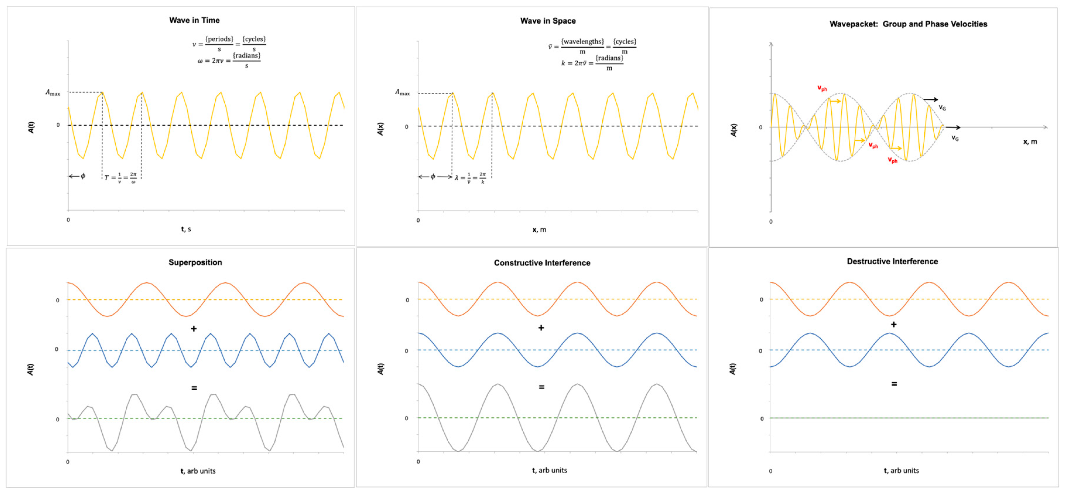
Figure 2.
(Lower) The Dual Slit Experiment demonstrates Wave-Particle Duality and the need for complex probability amplitudes in QM. Two identical high, narrow slits A and B of width (e.g., 0.035 nm) are cut into an impermeable partition a short horizontal distance (e.g., 0.4 nm) apart. Behind the barrier, an electron gun fires electrons of de Broglie wavelength (e.g., 2.75 pm) thru A and/or B at intensity . After traversing distance (~1 m) each electron impinges on a screen uniformly implanted with detectors. One measures the horizontal (coordinate ) distribution of electron impacts over a short distance (e.g., 10 mm). (Upper) the number of impacts at each in a given time interval is proportional to the electron beam intensity and to the probability of an impact at . If A is open and B covered, trace (dark blue) results. If A is covered and B open, we get the same curve shifted right (; dark red). But if both slits are open, we get (tan), a series of sharp peaks and troughs. Regardless of which slit(s) are open, always and only discrete single-electron impacts are registered at the screen. This suggests that electrons are CM particles. The form of , , and , however, belies this. If electrons were CM particles, would be a line segment of width and constant intensity directly across from A and likewise for . would consist of both segments separated by . In reality, while and do show most electrons impinging immediately opposite each slit, many electrons impact left and right of the slits. The real and are diffraction patterns. Diffraction is the well-known bending of CM waves as they pass thru apertures, like Slits A and B. The form of and is a relative of the sinc function (). is a more complicated sinc. It exhibits both diffraction and interference (Figure 1). The latter would occur if electrons emerged from A and B as coincident waves that interfered constructively and destructively to yield peaks and troughs, again CM wave behavior. Thus, , , and suggest electrons are waves. If so, what are they waves of? One guess is they are waves of probability itself, but this is not quite accurate. The laws of probability say that, if electrons moved in probability waves, for both slits open the distribution should be simply (teal). For probabilities by definition are always positive real numbers. Adding two of them could never produce the troughs in the observed interference pattern. Thus, the actual distribution . The actual is obtained by treating the electron as a wave not of probability but of probability amplitude . is a complex number that, when multiplied by is proportional to a probability, e.g., , , and . I.e., we only reproduce the empirically observed interference pattern by adding complex and (and multiplying by the conjugate), not by adding real probabilities. Thus, the Dual-Slit Experiment demonstrates CM wave and CM particle behavior of QM particles and the necessity of complex probability amplitudes to describe them. (Modified from Feynman & Hibbs 2010; curves not drawn to scale.).
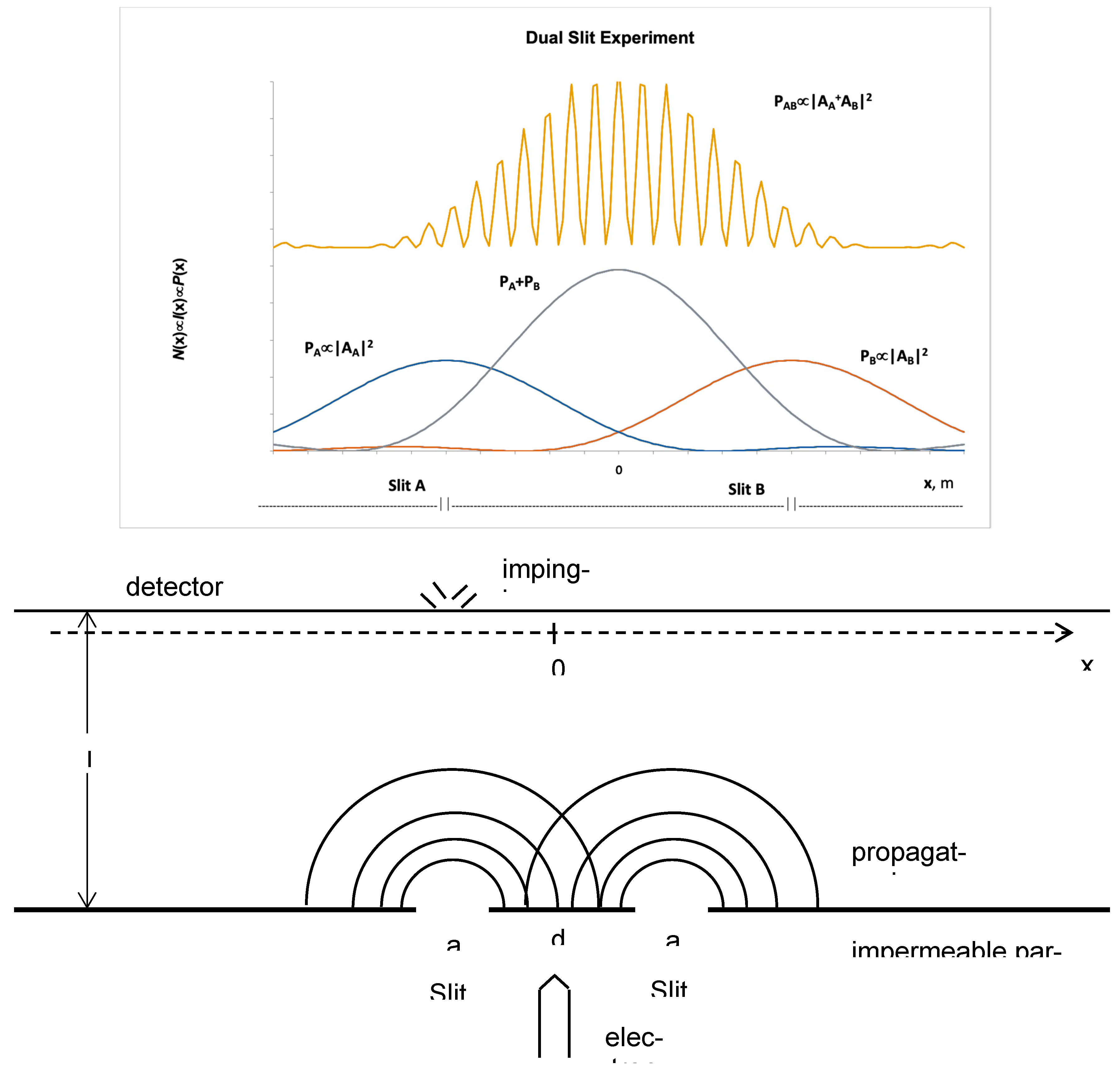
Figure 3.
This Heisenberg Supermicroscope aims to measure both position and momentum (short solid left-pointing arrow) exactly for a quantum particle of known mass moving along a 1D line. Simple-mindedly, a lamp shines light (wave and thin solid arrow descending from left) onto the particle. The light collides with the particle and reflects (wave and dashed arrow ascending right) to a lens where it forms an image. On the image we measure by counting hash marks on a graticule and momentum as marks passed per second times . With this technique, no shorter than the wavelength of the light can be measured, i.e., , the uncertainty of . Per Eq. (4), light itself, moreover, has momentum that makes the particle recoil (short dashed right-pointing arrow) upon collision. This changes its original velocity inducing an uncertainty into the momentum. To minimize and we try using the shortest wavelength and weakest light possible. But in QM, the weakest light deliverable is 1 photon. A photon has . Hence, the shorter and therefore the smaller , the larger and therefore the greater . I.e., there is a precision trade-off between position and momentum, calculated by Heisenberg as . By this Heisenberg Uncertainty Principle, the taproot of QM, and can never both be 0. We can never know everything about a quantum system.
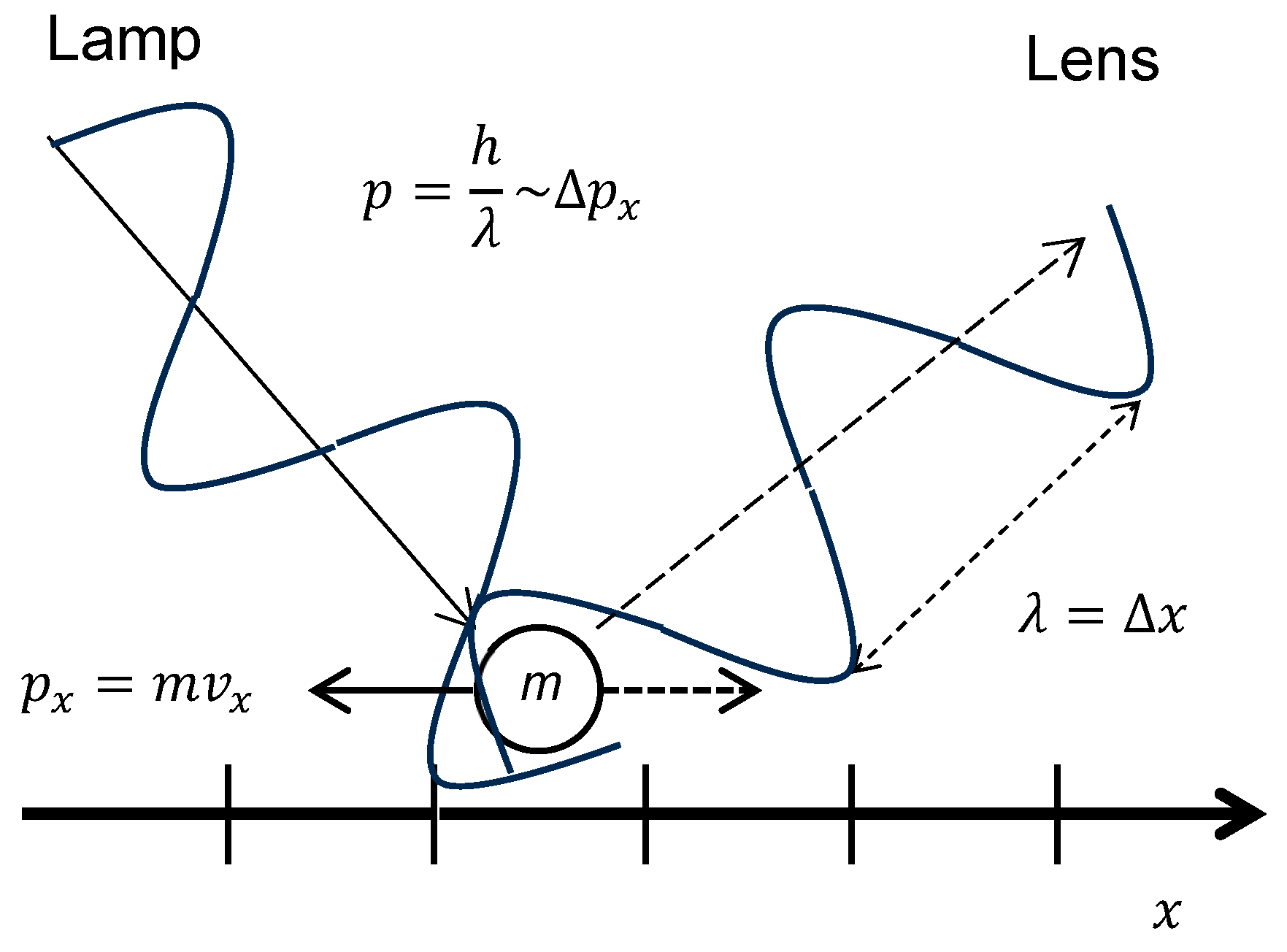
Figure 4.
Ideal probability distributions of experimental results in CM and QM. Distributions are across numerous identical measurements of 1D linear momentum () of one particle in the same state, respectively, of one measurement each of many particles in that state. The frequency , equal the probability , of finding a given value of is the number of measurements with that value per total number of measurements . (Left) in CM, the particle state has a single, certain momentum value, e.g., (arbitrary units). Every measurement returns . The probability distribution is a spike: 100% of measurements have ; 0 have any other value. The most probable value, the expectation value , i.e., the mean, average, or first moment-of-the-distribution, is . The second moment-of-the-distribution, roughly its width, is the uncertainty, . Hence, the CM distribution is determined by its first moment. (Center) even in an ideal quantum system, a particle has no single certain momentum value. Each measurement can return a different value than the last. The values are quasi-random; their probability distribution derives from the quantum state of the system. A Gaußian distribution is shown as example (though most quantum distributions are non-Gaußian). The expectation value is again . But the uncertainty is not 0, by the Heisenberg Principle it is . This uncertainty is a parameter shaping the distribution . Now the expectation value has probability < 1; instead, the sum of the probabilities of all possible values across , i.e., the area under the distribution curve, equals 1. This normalization condition implying the particle must return some (real-number) value for every measurement ties QM to the empirical world. (Right) quantum system with a probability distribution of measured values of a different observable with discrete eigenstates. In this (common type of) QM system, not 1, not infinitely many, but a finite number of specific values of (and no others) are allowed. These values are supplied by , by Process 2. They are the eigenvalues of and are quantities an instrument can read or a human can perceive. The quantum state , which can neither be measured nor perceived, supplies the probability of measuring each . I.e., shapes the distribution and reflects quantum randomness (Process 1). Each corresponds to a (normalized) eigenstate of in the Hilbert space of . The expansion coefficients express how much (normalized) overlaps with each , . Post-measurement, the quantum system slips into the quantum state of whichever happens to be measured. Thus, multiple measurements of an observable in QM return probability distributions rather than certain values. Individual outcomes result from independent contributions from the observable (Process 2) and the quantum state (Process 1). A different could change the values of and raise or lower the probabilities . In particular, upon measurement, . For , we then have and a CM probability distribution . I.e., repeated measurement, no matter how often, always yields .
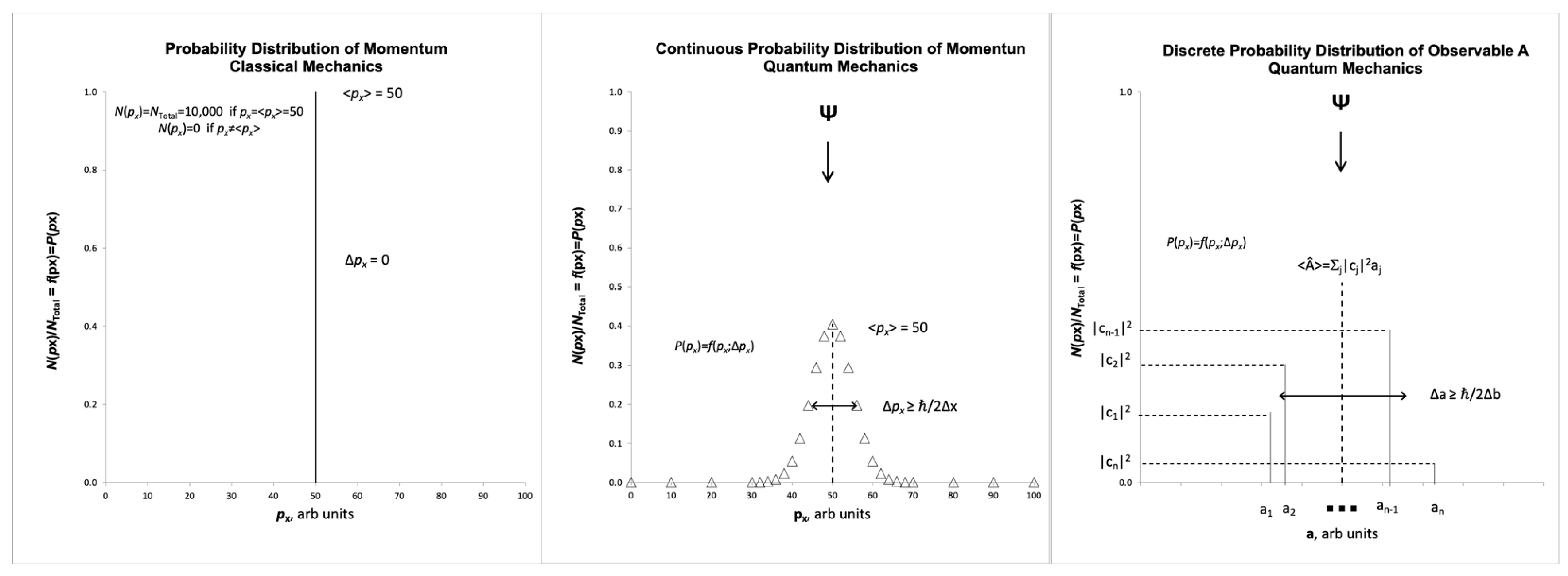
Figure 5.
Aspects of quantum states on the complex plane. “1” designates the real, “i” the imaginary axis. (Left) quantum states add (superpose) in the manner of waves or complex vectors. Quantum states and sum to quantum state . The probabilities of , and are proportional to , and , respectively. I.e, they each depend on the modulus and not the phase of the respective quantum state. But now rotate ccw by angle by multiplying it by phase factor The modulus of , and therefore the probability, of the quantum state are unchanged by this transformation; . Yet, the sum has both a different phase and a different modulus than . The latter implies . In this manner, relative phase does impact measurement when two or more vectors are superposed. Or when one or more components of a composite quantum state evolve to acquire a relative phase with respect to the others. (Modified from Bowman 2008.)(Right) why a probability amplitude or quantum state in 1D is like a “square-root” of a probability. In the case of a system of definite energy , a quantum state is a vector on the complex plane. The vector has constant radius . Its phase, the angle it makes with the real axis, varies with time as , with its frequency of uniform rotation in a circle centered at the Origin. The probability of observing the system in state is proportional to . This is independent of the phase. Since every phase contributes equally to the probability of , it is reasonable to make this probability proportional to the area of the circle . This area is something all phases also contribute to equally. Hence, . While probability is thus akin to an area on the complex plane, the modulus of the probability amplitude itself is a length. Since a length by nature is a square-root of an area, it seems reasonable that is something like a square-root of a probability. This may be a way to render the elusive character of the probability amplitude more comprehensible.
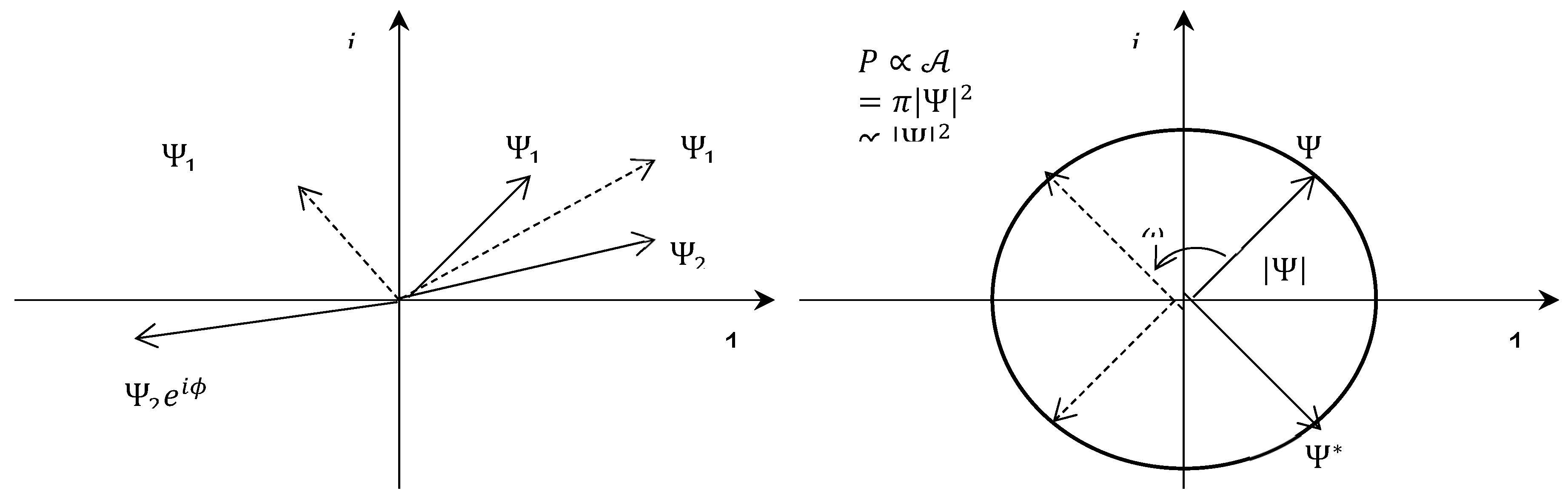
Figure 7.
One way to visualize complex Hilbert space. “1” designates a real, “i” an imaginary axis. Each quantum state has its own real and imaginary axes. Thus quantum state has a real axis and an imaginary axis perpendicular to it . Likewise, quantum state has real axis and perpendicular imaginary axis . A quantum state is defined only up to a physically irrelevant phase factor, meaning a factor that does not affect the probability distribution. Therefore, it is often acceptable to let the pure real state, the phase 0-state, stand-in for the entire complex quantum state. Thence, a Hilbert space, if drawn at all, is usually drawn using only pure real quantum states as coordinate axes. As discussed in Figure 5, non-zero phases are important in calculating superpositions of quantum states, inner products, adjoints, etc. In quantum systems of definite energy, the quantum state rotates about the complex plane over time in a circle centered on the Origin at constant frequency . Other quantum systems can be distributed in space at constant spatial frequency , etc. An oft neglected point is that each quantum state can rotate at its own frequency. Thus, e.g., if the energy observable of the system has eigenvalues , , will rotate at , and at .
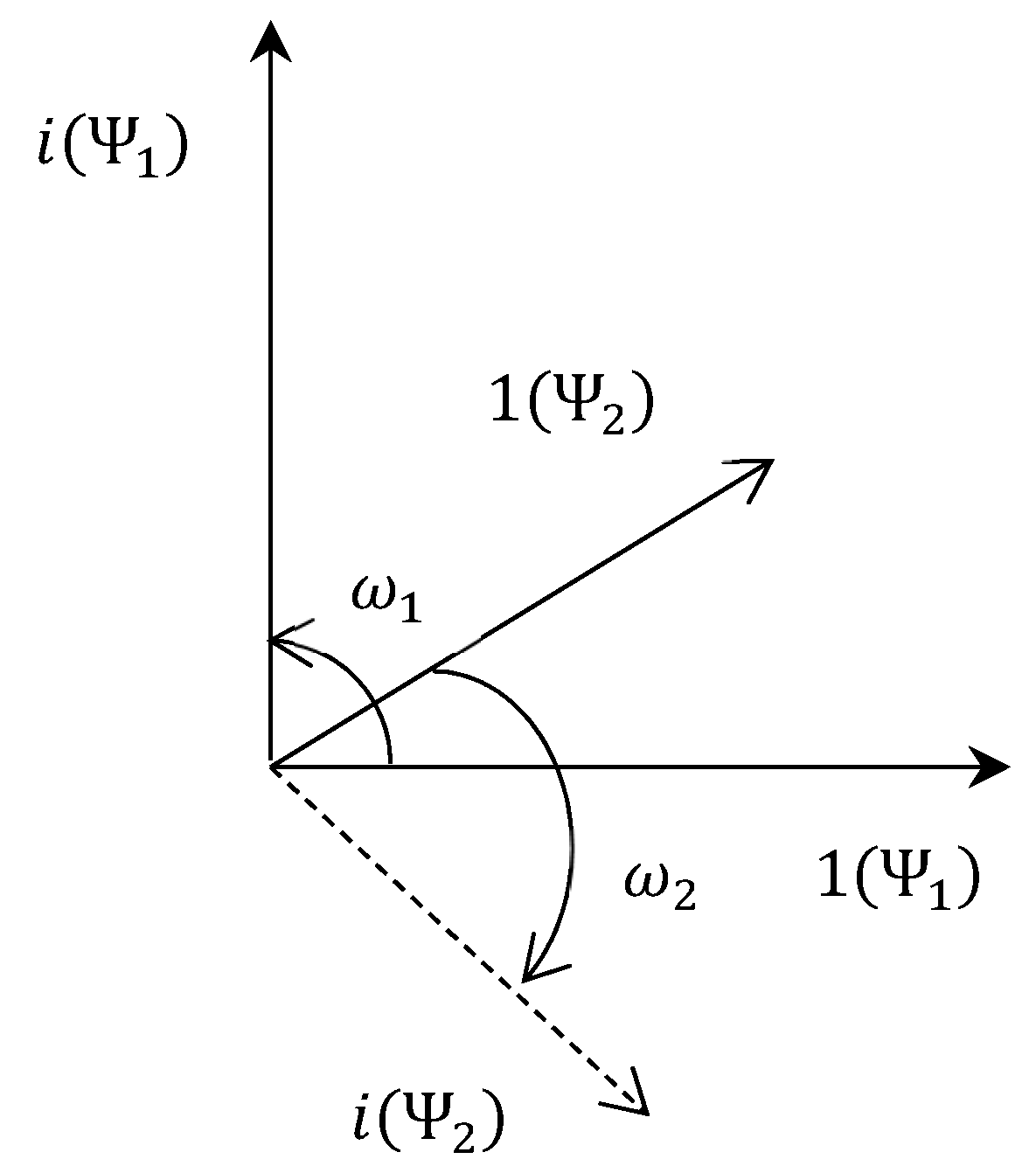
Figure 8.
How the apparatus dictates the eigenvalues (possible outcomes) of an experiment. (Upper left) flipping a coin, the apparatus is the air, and a tabletop. The tabletop forces the falling coin into the states heads (H) with eigenvalue or tails (T; ), where our outcome is the ccw angle the coin makes with the tabletop. The same experiment with a die (upper right) has six equiprobable outcomes, i.e., the system itself provides the primary probability distribution. (Middle) if our table has slopes and a plateau, we can measure heads-up states and tails-up states . The table edges enhance the probability of ; influence of the apparatus on the distribution. (Lower) if our apparatus consists of air and blitz camera, we can capture infinitely many states of the system with eigenvalues .
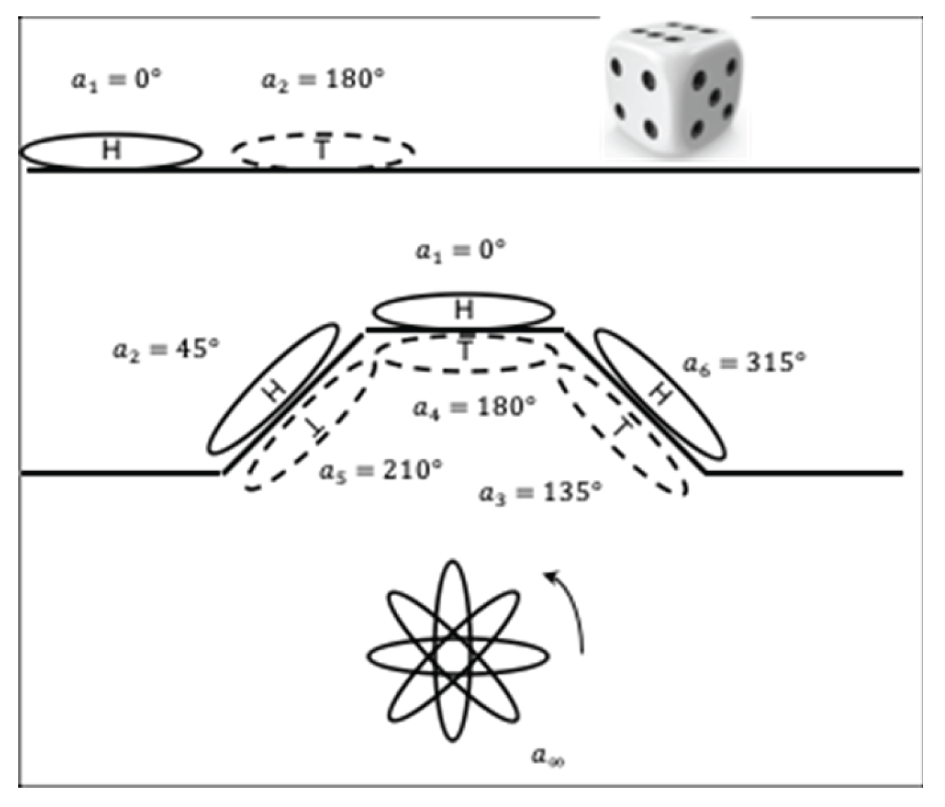
Disclaimer/Publisher’s Note: The statements, opinions and data contained in all publications are solely those of the individual author(s) and contributor(s) and not of MDPI and/or the editor(s). MDPI and/or the editor(s) disclaim responsibility for any injury to people or property resulting from any ideas, methods, instructions or products referred to in the content. |
© 2025 by the authors. Licensee MDPI, Basel, Switzerland. This article is an open access article distributed under the terms and conditions of the Creative Commons Attribution (CC BY) license (http://creativecommons.org/licenses/by/4.0/).
Copyright: This open access article is published under a Creative Commons CC BY 4.0 license, which permit the free download, distribution, and reuse, provided that the author and preprint are cited in any reuse.


