
Submitted:
17 November 2025
Posted:
18 November 2025
You are already at the latest version
Abstract
A Hermite-based framework for reliability assessment within the limit state method is developed in this paper. Closed-form design quantiles under a four-moment Hermite density are derived by inserting the Gaussian design quantile into a calibrated cubic translation. Admissibility and implementation criteria are established, including a monotonicity bound, a positivity condition for the platykurtic branch, and a balanced Jacobian for the leptokurtic branch. Material data for the yield strength and ductility of structural steel are fitted using moment-matched Hermite models and validated through goodness-of-fit tests. A truss structure is then analysed to quantify how non-Gaussian input geometry influences structural resistance and its corresponding design value. Variance-based Sobol sensitivity analysis demonstrates that departures of the radius distribution towards negative skewness and higher kurtosis increase the first-order contribution of geometric variables and thicken the lower tail of the resistance distribution. Closed-form Hermite design resistances are shown to agree with numerical integration results and reveal systematic deviations from FORM estimates, which rely solely on the mean and standard deviation. Monte Carlo simulation studies confirm these trends and highlight the slow convergence of tail quantiles and higher-order moments. The proposed approach remains fully compatible in the Gaussian limit and offers a practical complement to EN 1990 verification procedures when skewness and kurtosis have a significant influence on design quantiles.
Keywords:
Hermite distribution
; structural reliability
; design quantiles
; limit states method
; firstorder reliability method
; non-Gaussian modelling
; skewness
; kurtosis
; Sobol sensitivity analysis
; Monte Carlo simulation
MSC: 65C50; 60H99; 82B31
1. Introduction
In structural reliability, EN 1990 [1] adopts a simplified approach that uses only the mean and standard deviation to derive design values via the First Order Reliability Method (FORM). The Standard [1] introduces three basic probability distributions: the Gaussian, the lognormal, and the Gumbel probability density functions (pdfs). Structural resistance is most often modelled using the Gaussian [2,3] or lognormal [4,5] pdfs, while the Gumbel pdf is applied to represent extremes of dynamic response [6,7] or long-term, single-variable load actions [8,9,10,11]. In practice, EN 1990 does not prescribe a specific mapping of variables to probability distributions and provides closed-form design expressions only for these three two-parameter families, see Figure 1. The target reliability must therefore be demonstrated using a distribution and parameter values that reproduce the observed data. However, two-parameter pdfs may be inadequate for this purpose, see, e.g., [12,13,14].
Numerous studies have shown that the actual probability distribution of structural resistance often departs from simple Gaussian or lognormal models [15,16]. For example, recent material tests indicate that different failure modes or material properties may follow distinct distributions — tensile strength may fit a normal law, whereas compression or shear strength may follow Weibull or lognormal laws [15]. Strength data for high-performance fibres and polymers provide further evidence that, even when statistical tests “cannot reject normality”, the true strength histograms deviate from the ideal bell-shaped Gaussian curve [16]. In advanced composites, manufacturing defects can produce fat-tailed or skewed resistance distributions rather than the assumed thin-tailed form [17]. Similarly, accelerated ageing or damage can alter an initially normal resistance distribution into a Weibull-type distribution with heavier tails [18]. In such cases, structural strength variables exhibit skewness, heavy tails, or even multimodal behaviour, departing significantly from the classical normal or lognormal assumptions [17,18].
There are measurement cases in which the data distribution is only approximately Gaussian. However, when slightly larger deviations characterised by higher skewness or kurtosis occur, alternative distribution models should be considered [19,20]. Such cases have been observed both in experimental data [21,22] and in model outputs in engineering [23,24]. In both cases, the histogram approaches a bell curve, and the higher moments (skewness and kurtosis) approach zero or small values typical of a normal distribution. For such models, a suitable option is to employ a four-parameter Hermite probability density function (pdf) [25].
This article analyses the limit states of load-bearing structures using a Hermite model [25], which enables calibration to measured data exhibiting non-negligible skewness and kurtosis. The focus is placed on situations where the shape of the probability distribution materially influences the lower design quantiles of resistance and, consequently, the required level of reliability. Sobol sensitivity analysis is employed to quantify the contribution of each input variable and their interactions to the variance of the model output. In addition, it is used to evaluate how different choices of input probability distributions affect overall model sensitivity.
2. Hermite Models for Tail-Sensitive Reliability
Many studies report that the probability distributions of loads and resistances deviate from the Gaussian law and can exhibit non-zero skewness and kurtosis [26,27,28,29]. These higher-order moments can significantly influence failure probabilities and the reliability index [30,31]. Consequently, computed results depend on the assumed input distributions, as demonstrated for wind-loaded truss towers [32]. Therefore, more advanced probabilistic models are required.
The Hermite translation method serves as a tail-aware default when departures from normality are of interest. Its third-order mapping transforms a Gaussian variable into a non-Gaussian one, with shape parameters controlling skewness and kurtosis [25,33,34]. Evidence from wind engineering shows that the Hermite probability density function (pdf) improves tail representation for both mildly and strongly non-Gaussian pressure data on low-rise buildings [35]. The Hermite pdf has also been employed to obtain moment-based peak factors for pressure and displacement responses [36,37]. When full probability distributions are unavailable, reliability assessment and partial safety factor calibration can utilise moment methods based on the third to fifth moments [30,31,38]. Correlated inputs can be addressed using an L-moment-based normal transformation [39]. These approaches do not require full distributions and more faithfully capture non-Gaussian behaviour. As a general alternative, a unimodal four-moment density can represent a wide range of skewness and kurtosis and connects to both normal and lognormal limits [40].
Extensions of Hermite models target small to moderate deviations from normality. An adaptive Hermite model using probability-weighted moments estimates extreme value distributions for seismic reliability, while asymptotic analysis clarifies the monotonic domain and establishes connections to Gram–Charlier behaviour [41,42]. L-moment-based Hermite mappings enable efficient simulation of non-Gaussian random fields in structural [43] and geotechnical applications [44]. When higher-order moments are required but full distributions are not available, skewness and kurtosis can be estimated through a regression-based adaptation of the Cornish–Fisher expansion to improve shape recovery for asymmetric or heavy-tailed data [45]. In parallel, a flexible four-moment distribution employing a cubic normal transformation covers a broad region of the skewness–kurtosis plane and connects to the normal and lognormal limits [46]. For non-stationary, non-Gaussian responses, a unified Hermite mapping provides analytical mean upcrossing rates, and complementary studies quantify the transmission of kurtosis from excitation to response under both stationary and non-stationary loadings [47,48,49,50]. Hermite polynomial models have also been integrated into dynamic reliability formulations under non-Gaussian excitation [51].
Fatigue assessment is particularly sensitive to non-Gaussian features, as damage accumulation is driven by high-amplitude cycles in the distribution tails. Skewness and kurtosis can be embedded into damage estimators through Hermite-based mappings when full distributions are unavailable. For instance, Hermite transformations have been applied to fatigue damage estimation in broadband non-Gaussian processes using a conditional probability approach [52]. Time–frequency frameworks for non-stationary loading employ spectral methods for non-Gaussian processes and support fatigue evaluation [53]. Fast modal-domain estimators of response kurtosis enable efficient assessment of non-Gaussian effects in full finite element models used for random vibration fatigue [54]. Under simultaneous non-Gaussian processes, bias correction incorporating kurtosis improves fatigue damage estimates compared with linear summation [55]. For floating offshore wind turbine blades, non-Gaussian wind fields have been shown to reduce predicted fatigue life relative to Gaussian assumptions [56]. Fatigue in steel plate welded joints has also been evaluated using both non-Gaussian parametric and non-parametric formulations [57].
Direct applications of the Hermite pdf, or its explicit use for uncertainty modelling, span theoretical developments [33,34,41,42,47], simulation and random fields [43,44,58], wind loading and peak factor estimation [35,36,37,59], and reliability and fatigue analysis [25,51,52,56]. Several studies have employed quartic-order Hermite polynomial mappings to transform Gaussian variables into prescribed non-Gaussian distributions [31,44,58,59]. Although the quartic Hermite polynomial can improve the shape of the pdf, its monotonic domain is assessed locally and may be narrower over the practical working range. In contrast, the cubic model provides a transparent and easily verifiable monotonic boundary [44,59]. This article employs a cubic Hermite pdf model, the derivation of which is presented in the following chapter. The cubic model is suitable for formulating design quantiles and can surpass the accuracy of design values obtained using the classical FORM method.
3. Hermite Model: Map, Densities, and Properties
The Hermite translation model is introduced to represent moderate deviations from Gaussian behaviour while maintaining a compact four-parameter description defined by the mean, standard deviation, skewness, and kurtosis [25]. Throughout this chapter, a real-valued random variable X with finite moments is considered. The mean and variance are denoted by μ and σ2. The central and standardised moments follow the conventions stated below.
For a Gaussian variable, one has α4=3, departures from Gaussian kurtosis are therefore captured by α4−3. Under these conventions, the standardisation in Equation (3) maps the observations to zero mean and unit variance, while the Hermite translation in Equation (4) introduces controlled adjustments to symmetry and tail weight through the calibrated coefficients defined in Equations (5)–(6) and Equation (14).
3.1. Polynomial Map and Parameterisation
A random variable X with mean μ, standard deviation σ, skewness α3, and excess kurtosis α4 is approximated by transforming a standard normal variable U∼N(0,1).
The standardised observation is
which has zero mean and unit variance. The Hermite translation model introduces a unit-variance surrogate defined as
where H2(U)=U2−1 and H3(U)=U3−3U are the second- and third-order Hermite polynomials, respectively. The third- and fourth-order base coefficients h3 and h4 are given by
where the constant k is a variance rescaling factor chosen such that V(Y)=1. Because the Hermite polynomials are orthogonal under the Gaussian inner product, E[U Hn(U)]=0, the centring is preserved, i.e. E(Y)=0. Equations (3)–(5) define the common basis of the model. The branch-specific calibrations , and correction factors kt are introduced below.
3.2. Density Derivations
3.2.1. Lower-Branch Density (α4≤3)
For α4≤3, the Winterstein calibration is applied:
Dividing Equation (4) by kt gives the working, dimensionless mapping:
The density of Y follows from the change-of-variables formula:
and is obtained perturbatively for , ≪ 1.
Applying a first-order Neumann inversion to Equation (7), and using the scalar rule (1+a)-1 ≈ 1-a for ∣a∣≪1, the map U↦U+ε(U) can be inverted to first order as U≈y−ε(y). This results in:
Differentiating Equation (7) gives:
where U is replaced by y to first order. Substituting Equations (9)–(10) into Equation (8) then gives:
For a non-standardised X, it is convenient (and consistent with the calibration) to evaluate the model at:
whence, by the one-dimensional change-of-variables rule,
Equations (9)–(13) define the lower-branch pdf used in practical applications. The approximation remains accurate while ∣α3∣≪1 and the kurtosis surplus α4−3 is non-positive or only mildly positive.
3.2.2. Upper-Branch Density (α4>3)
For α4>3 the calibrated moments are defined as:
The working mapping remains as in Equation (7), with ,and kt obtained from Equation (14). In this branch, the inverse mapping U(y) can be obtained in the closed form. Let
and introduce the shift U=X−A. Substituting into Equation (7) yields the depressed cubic form:
where the shift U=X−A removes the quadratic term, yielding the depressed cubic with coefficients Q and ξ defined in Equation (15).
Define
By applying Cardano’s formula and selecting the principal real cube roots, the real solution for U(y) is obtained as:
This expression for U(y) satisfies Equation (16) (with X=U+A) and, consequently, the original mapping in Equation (7).
The Jacobian dU/dy is obtained by differentiating Equation (18). From Equations (15) and (17),
and differentiating Equation (18) followed by the substitution of Equation (19) yields
Hence, from the change of variables relation in Equation (8), the probability density function is given by
where U(y) is given by Equation (18) and A, B, Q, ξ, R are defined in Equations (15)–(17). For a non-standardised variable X,
Equations (18)–(22) are exact; no terms are neglected. The use of principal real cube roots in Equation (18) is justified by the condition R±ξ≥0, which ensures continuity of U(y) across ξ=0.
3.3. Properties and Admissible Sets
This section summarises the conditions under which the Hermite pdf, derived in the previous sections, behaves well numerically and accurately reproduces the prescribed moments. The guidance is expressed in the native parameters α3 and α4 through the calibrated quantities ,and kt defined above.
3.3.1. Non-Negativity and Monotonicity
The lower-branch density in Equation (13) is a first-order change-of-variables approximation; neglected terms are of order O(). Moment matching is therefore only first-order accurate while ,≪ 1. Using the calibrations of Equation (6), large values of ∣α3∣ or ∣α4-3∣ push the approximation outside its linear regime and bias the empirical moments by terms of order O().
Positivity of the first-order form in Equation (13) holds as long as the bracket term remains non-negative over the range of interest. The bracket in Equation (11) is
For platykurtic cases , the corresponding parabola opens upward, and its minimum occurs at
A sufficient condition for ∣dU/dy∣ ∝ g(y)>0 over the effective range is therefore
When ≪ 1, Equation (25) reduces to a transparent rule of thumb,
obtained by substituting ≃h3=α3/6 and ≃h4=(α4−3)/24.
Violation of Equations (25)–(26) identifies regions where g(y)<0. In exact theory, this would create negative lobes of fY in the far tails. In numerical implementations, such tails are often clipped to zero, which reduces the total mass ∫fY and shifts the empirical moments.
In practice, for a given pair α3, α4, the recommended procedure is to compute and and test Equation (25). If it is marginally violated, g(y)≥0 should also be verified over the effective range of ∣y∣. Failure of either test indicates that the first-order model may require post-normalisation (which perturbs moments) or the adoption of a different pdf.
The upper-branch density defined by Equations (21)–(22) is exact, employing the Cardano real root of the depressed cubic (16). The Jacobian factor (20) follows by direct differentiation, with no truncation error. Two numerical aspects merit attention.
First, monotonicity of the mapping U↦Y is guaranteed while the cubic has a single real branch. In terms of α3 and α4, this corresponds to the classic engineering criterion
beyond which the cubic becomes multi-valued and the Cardano transformation no longer defines a valid pdf.
Second, although Equation (20) remains finite for all admissible parameters (since R±ξ≥0), near R≈ξ≥0 the individual factors (R±ξ)2/3 can become large. The balanced product in Equation (20),
avoids catastrophic cancellation and ensures numerical stability on implementation.
3.3.2. Realised Moments
This section presents the closed-form expressions for the realised first four moments of the Hermite pdf and explains how inputs may be specified either through the native parameters (μ, σ, α3, α4) or, on the upper branch, directly via the target moments (μ*, σ*,,).
The standardised surrogate variable Y defined in Equation (4) is employed together with the branch–specific calibrations of ,and the scaling factor kt given in Equations (6) (lower branch) and (14) (upper branch). The location–scale moments of a non-standardised quantity X=μ+σY then follow directly from those of Y.
On the upper branch (α4>3), the variance rescaling defined in Equation (14) ensures exact centring and unit variance due to the orthogonality of the Hermite basis,
Consequently,
Because Y is expressed as a polynomial in the Gaussian variable U, the realised skewness and kurtosis are obtained in closed form as functions of (,). These expressions are exact for the upper branch. Denoting and as defined in Equations (6) and (14), the realised skewness and kurtosis are given by
The density on the upper branch is obtained by the exact Cardano inversion using the balanced Jacobian from Equation (28). When the target shape moments (,) are prescribed, the coefficients (,) can be recovered through a stable inversion of Equations (31) and (32). The forward relations given in Equation (14) provide an initial estimate that is first-order accurate in (α3, α4−3). Admissibility of the upper branch follows from the monotonicity criterion in Equation (27). It can be noted that similar explicit relations between higher-order moments and distribution parameters have recently been derived for the Weibull pdf and used to compute design quantiles in hydrological design [60].
On the lower branch, the Winterstein calibration in Equation (6), combined with the first-order Neumann inversion and the change of variables in Equation (13), yields an approximate density. In this regime, only first-order preservation of the first two moments is achieved,
Consequently,
Using Equations (31) and (32) with the lower-branch values of (,) yields (,) to first-order; higher-order deviations increase with ∣α3∣ and ∣α4−3∣. Practical admissibility and non-negativity on the lower branch are governed by Equations (23)–(26), with the serviceability rule given by Equation (26).
Let θ=(μ, σ, α3, α4) denote the input parameters used to evaluate the Hermite pdf through Equation (4) and the branch-specific calibrations in Equation (6) or (14). Denote by
the realised moments computed from the resulting density fX(⋅∣θ). For the lower branch M(θ)−θ is of order O(,,). For the upper branch, the inversion is exact and the relations in Equations (31) and (32) express the realised skewness and kurtosis precisely as functions of (,).
Two short illustrations follow.
Lower branch: For the inputs θ=(0, 1, 0.05, 2.95), Equations (31) and (32) yield ≈0.049996 and ≈2.95334. Numerical integration of the pdf over the interval [−19, 19] yields ≈0.0503 and ≈2.9563, reflecting higher-order effects inherent to the first-order formulation.
Upper branch: For the inputs θ=(0, 1, −0.1, 3.1), numerical integration agrees with Equations (31) and (32) for the prescribed pair (,). When the forward relations of Equation (14) are used, the realised kurtosis ≈3.113 slightly differs from the target due to the first-order character of that calibration. Solving Equations (31) and (32) for (,) enforces =-0.1 and =3.1 within numerical precision.
For reporting purposes, the moments obtained from Equations (31) and (32) should be regarded as the reference values, while those computed by numerical integration of the lower-branch pdf may serve as a first-order consistency check.
3.4. Implementation and Workflow
Equations (25)–(28) provide analytical criteria that define the admissible regions in α3 and α4, ensuring both positivity and monotonicity of the Hermite pdf. For practical applications, these conditions must be embedded within an implementable computational routine. The Pascal/Delphi function presented below encodes both branches of the density, using the Winterstein calibration (Equation (6)) for α4≤3 and the exact Cardano inversion (Equations (18)–(22)) for α4>3. The Jacobian factor is implemented in the balanced form given by Equation (28), which prevents numerical cancellation errors in the vicinity of R≈ξ.
The structure of the routine reflects the admissibility conditions. When α4≤3, the Neumann inversion is truncated at first order, consistent with the approximation in Equation (13). When α4>3, the exact cubic root is employed, and validity requires compliance with the monotonicity criterion of Equation (27). In both branches, the Gaussian kernel ϕ(U) is evaluated once, and rescaling by kt ensures unit variance. A defensive clamp at the end of the routine enforces non-negativity of the pdf and prevents spurious negative values under extreme input conditions.
The Pascal (Delphi 6) implementation of the Hermite pdf is provided in Appendix A.
This implementation enables the direct numerical evaluation of the Hermite pdf without further algebraic manipulation. In practical applications, the computational workflow proceeds as follows:
- Compute , and kt from α3 and α4.
- Select the branch: apply the Winterstein correction for α4≤3, or the Cardano inversion for α4>3.
- Verify the admissibility conditions, Equation (25) for the lower branch or Equation (27) for the upper branch.
- Evaluate the density using the function above.
If the admissibility conditions are violated, the Hermite pdf cannot be used directly. In such cases, an alternative parametric or non-parametric model, which is better suited to the empirical histogram, must be adopted.
4. Fitting and Validation on Materials Data
Recent experimental studies on reinforcing steel bars, welded joints and cementitious composites report non-Gaussian measurement profiles characterised by non-negligible skewness and excess kurtosis [61,62]. As a result, strength and geometric characteristics are often modelled using Weibull, lognormal or gamma distributions [63,64,65,66]. In fibre-reinforced polymer rods and in fibre-reinforced concrete exposed to high temperatures, Weibull fits effectively capture right-skewed tails and summarise the design-relevant variability [63,64]. For metakaolin masonry blocks and large regional datasets of green concrete, lognormal or gamma laws frequently provide the best or at least competitive fits [65,66]. In rolled steels and butt-welded seams, empirical skewness and kurtosis often deviate substantially from the normal benchmark, with several cases exhibiting kurtosis greater than three, motivating the explicit use of non-Gaussian modelling [26,61,62].
For many experimental datasets, the Hermite pdf can serve as an extension of the Gaussian model that accommodates small but non-zero skewness and variable excess kurtosis. For example, in weld toe geometry and reinforcement height distributions that remain close to symmetric yet exhibit mild excess kurtosis, a moment-matched Hermite fit can be applied instead of switching to lognormal or gamma families [61]. For reinforcing steel, where the sign of skewness varies across production lots, both positive and negative skewness can be represented within a single parametric family while preserving the observed variance and kurtosis [26]. For regional concrete datasets that are approximately normal, small departures from symmetry and tail weight can be captured using a parsimonious Hermite approximation that retains the Gaussian baseline for interpretability [66].
In the following section, Hermite pdfs are fitted to our experimentally obtained material characteristics of structural steel [67,68], which exhibit non-Gaussian skewness and kurtosis. The fits are validated using histograms and moment analysis.
4.1. S235 Yield Strength (Lower Branch)
In engineering practice, histograms of measured quantities may deviate, to varying degrees, from the Gaussian pdf. An illustrative example is provided by the yield strength fy of structural steel grade S235 [67]. Based on n=562 valid observations of fy, the sample statistics were estimated as mean of 297.3 MPa, standard deviation of 16.8 MPa, skewness of 0.325, and kurtosis of 2.5415 [67].
For a platykurtic input, the lower-branch relations given by Equations (6) to (13) apply. The rule in Equation (26) gives ≪4.5(3−α4), and the non-negativity check based on Equations (23)–(25) is satisfied across the effective range; hence, admissibility is confirmed.
When the pdf is evaluated using the input θ=(297.3 MPa, 16.8 MPa, 0.325, 2.541), the realised moments of the resulting Hermite pdf are M(θ)=(297.429 MPa, 16.207 MPa, 0.904, 3.821), where numerical integration was performed over the range [μ−19σ, μ+19σ]. The Kolmogorov–Smirnov (KS) test indicates a lack of fit with p=0.00148<0.05; see the red curve in Figure 2. This behaviour is consistent with the first-order character of Equations (9)–(13).
After a minor parameter refinement within the admissible region, θ=(297.5 MPa, 17.6 MPa, −0.071, 2.349) produces realised moments M(θ)=(297.337 MPa , 16.818 MPa, 0.328, 2.544), which closely approximate the sample moments. The KS test then reports p=0.2965>0.05; see the green curve in Figure 2. Both parametrisations satisfy Equation (26) and the positivity condition in Equation (25). The improved fit results from compensating for the first-order truncation error inherent in Equations (9)–(13).
This structure ensures that the first four moments are taken into account while maintaining conceptual transparency. If the admissibility conditions are violated, the recommended fallback is to revert to the Gaussian pdf or to adopt an alternative model.
4.2. S235 Ductility (Upper Branch)
Ductility measurements for S235 steel, based on n=562 observations, are analysed. The sample moments are μ=37.8%, σ=2.9%, α3=−0.753 and α4=5.18. Since α4>3, the upper-branch formulation is applicable: calibration follows Equation (14), the exact cubic inversion is performed using Equations (18)–(22), and the Jacobian is evaluated in the balanced form given by Equation (28). The monotonicity requirement specified in Equation (27) is satisfied.
Using the sample moments directly as inputs θ=(37.8, 2.9, −0.753, 5.18) (red curve in Figure 3) yields the realised moments M(θ)=(37.8, 2.9, −0.751, 6.026) when evaluated either by numerical integration over the range [μ−19σ,μ+19σ] or by direct substitution into Equations (31) and (32). The discrepancy (,)≠(α3,α4) reflects the first-order nature of the polynomial translation in Equation (4). The Kolmogorov–Smirnov test gives p=0.0273<0.05; hence, the model is rejected.
A short refinement of the input parameters improves agreement between he realised and sample moments. With θ=(37.8, 2.9, −0.7605, 4.422) (green curve in Figure 3), the realised moments become M(θ)=(37.8, 2.9, −0.753, 5.180), which are very close to the sample moments. However, the Kolmogorov–Smirnov test still rejects the model at the 5% significance level. It can be noted that increasing the input kurtosis parameter to α4=7.0 while keeping μ≈37.8, σ≈2.9 and α3≈−0.762 yields p=0.121>0.05, i.e., non-rejection, but at the expense of a substantial deviation from the sample kurtosis.
A practical trade-off is implied: enforcing exact moment matching does not necessarily maximise agreement under the Kolmogorov–Smirnov criterion. Notably, in all configurations considered, the Hermite fits were not rejected by the Anderson–Darling goodness-of-fit test, indicating adequate tail behaviour despite the KS test’s sensitivity to central discrepancies for large n.
4.3. Extreme-Moment Inputs
This subsection examines inputs θ=(μ, σ, α3, α4) that lie outside the perturbative regime assumed in the derivation. In such cases, θ must be regarded as control parameters of the transformation rather than as guaranteed realised moments, and the resulting pdf fX(⋅∣θ) must be validated a posteriori. Validation includes checks for non-negativity and normalisation, admissibility via Equation (25) for the lower branch and Equation (27) for the upper branch, and consistency of the realised moments M(θ)=(μ*, σ*, , ) with the intended targets. Where discrepancies occur, a constrained numerical calibration of θ is required, followed by re-evaluation using Equations (13) for the lower branch or Equations (21)–(22) for the upper branch, with the balanced Jacobian defined in Equation (28).
For strongly platykurtic inputs (α4<3), the first-order representation of the lower branch, fY(y)≈ϕ(U(y)) g(y) with defined by Equations (11) and (23), governs admissibility and the shape of the pdf. When <0, the factor g(y) forms a convex parabola whose minimum occurs at ymin and reaches gmin as given in Equation (24). Positivity requires gmin>0, corresponding to the bound in Equation (25). This bound explains two features observed in Figure 4. Firstly, very small target kurtosis depresses the centre of g(y) and may create a double-humped pdf even when the mapping remains monotonic. Secondly, large values of ∣α3∣ shift the minimum of g(y) and tighten the constraint imposed by Equation (25). Consequently, extremely low kurtosis cannot be combined with large skewness without violating non-negativity. In the mild-departure limit, the transparent rule of thumb expressed by Equation (26) is recovered.
For leptokurtic inputs (α4>3), the upper branch employs the exact cubic inversion defined by Equations (18)–(22), and monotonicity reduces to the single inequality expressed in Equation (27). Because the right-hand side of Equation (27) increases with α4−3, larger magnitudes of ∣α3∣ become admissible as kurtosis increases. This behaviour is consistent with the broader family of attainable pdf shapes illustrated in Figure 5. The Jacobian remains finite when evaluated using the balanced product form in Equation (28). Nevertheless, even on this branch, the polynomial translation given in Equation (4) represents a cubic truncation. Consequently, the realised higher-order moments deviate from the input values once (α3, α4) move sufficiently far from (0, 3).
In practical modelling, the extreme-input regime can generate useful pdf shapes, including light-tailed or bimodal forms. The reliability of such fits depends on enforcing the admissibility conditions given by Equations (25)–(27), verifying the normalisation and non-negativity of fX, and, where necessary, numerically calibrating θ so that M(θ) satisfies the desired moment constraints while the pdf remains admissible.
5. Reliability Application
In EN 1990, design values are obtained from the mean and standard deviation using the FORM [1]. When full probability distributions are specified, design quantiles are typically derived from Gaussian, lognormal or Gumbel laws [1]. A review of the literature reveals no published calculation of the 0.12% quantile directly under a Hermite probability density function. Existing applications of the Hermite model have focused primarily on peak factor estimation [37], dynamic reliability [51], and fatigue assessment [53], rather than on code-level design quantile evaluation. Motivated by these gaps, the following section derives closed-form design quantiles under a Hermite density, allowing skewness and kurtosis to be incorporated consistently into the estimation of design quantiles.
5.1. Design Quantiles
5.1.1. EN 1990 Quantile
Let the structural resistance R and the load effect F be modelled as independent random variables with means μR, μF and standard deviations σR, σF, see, e.g., [69]. The performance function is defined as
Under the Gaussian baseline, the reliability index
leads to the failure probability Pf=Φ(−β). Eurocode practice compares β with a target reliability index βd (for the ultimate limit state: βd≈3.8, corresponding to Pf≈7.2⋅10−5).
Within FORM, the contribution of R and F to σZ is described by sensitivity factors αR, αF>0 (for independent normal variables αR=σR/σZ, αF=σF/σZ, some standards adopt fixed values, e.g., αR=0.8, αF=0.7 [1]). The design values are then expressed as
The reliability requirement is verified through the inequality of the design quantiles:
The design resistance Rd,FORM represents the lower Gaussian quantile at probability level
where, for the ultimate limit state, βd=3.8 and αR=0.8 are used for reliability class RC2 in [1]. This gives pd≈Φ(-3.04)≈0.0012.
The design load action Fd,FORM corresponds to the higher Gaussian quantile at probability level
Symbols α3, α4 denote skewness and kurtosis used in the Hermite pdf, while αR and αF are FORM sensitivity coefficients (weight factors) and must not be confused.
5.1.2. Hermite Quantile (Closed Form)
Let U∼N(0,1) and define the Hermite translation as
with branch-specific , and kt determined by (α3,R, α4,R) under the admissibility and monotonicity conditions stated earlier. The structural resistance is then
If T is strictly increasing (upper branch: exact, lower branch: valid in the small-departure regime), the cumulative density function (CDF) transforms as FR(r)=Φ(U(r)). Hence, the p-quantile is obtained by inserting the Gaussian p-quantile zp=Φ−1(p) into the forward map:
where zp=Φ−1(p). For design purposes in the FORM sense, retain the target probability content
and define the Hermite-based design resistance as
This expression reduces to the Gaussian design value Rd,FORM=μR−αRβdσR in the limit α3,R→0, α4,R→3, where ,→0 and kt→1. Examples of design quantiles for normalised distributions with μR=1 σR=1 are shown in Figure 6.
When the load effect F is modelled as non-Gaussian, the same construction applies using parameters (μF, σF, α3,F, α4,F) and coefficients ,,. The design quantile corresponds to pF=Φ(+αFβd) with zF=+αFβd, giving
which reduces to the Gaussian Fd,FORM as α3,F→0 and α4,F →3. In the present study, only Rd,HERM is used in the examples.
5.2. Case Study: Pin-Jointed Tie System
A pin-connected node is supported by two axially loaded ties and subjected to a vertical gravity force F>0, see Figure 7.
Small-displacement statics and perfectly pinned joints are assumed; self-weight and bending effects are neglected. Static equilibrium of the node gives
where and . The axial force in each tie under given vertical load is F1=F2=F by Equation (50).
Let fy1 and fy2 denote the yield strengths of the two steel ties, and A1 and A2 their respective cross-sectional areas. The axial load-carrying capacities are
where fy is expressed in MPa and A in mm2, giving NR in N. The vertical load action that brings tie i to its ultimate limit state follows from Equation (50):
The structural (system) resistance is governed by the weaker tie reaching yield first:
where (i = 1, 2) denotes the cross-sectional area of the solid circular bar with radius ri. Equation (53) is nonlinear, because the system resistance is governed by the weaker tie and the axial capacity of each tie depends on geometry and yield strength.
It can be noted, that comparable nonlinear input–output relations occur in nonlinear shell analysis [70,71], in the nonlinear reliability assessment of steel frames with Gaussian imperfections [31], and in nonlinear fatigue analysis under Gaussian loading [72]. Studies [31,70,72] show that nonlinear structural models with Gaussian input variables often yield non-Gaussian outputs due to the inherent nonlinearity of the input–output relationship. Skewness, kurtosis and other higher-order features of model output may therefore arise from the model itself, from the input distributions, or from a combination of both.
5.2.1. Inputs Random Quantities
Equation (53) is a function of four random quantities, where input vector is
and the model output is the structural resistance Y=R(X) obtained from Equation (53). In Equation (54), the four input variables are assumed to be mutually independent, and both members are assumed to possess identical statistical distributions of material and geometric properties.
The yield strength fyi is treated as a random variable described by the histogram shown in Figure 2. The green Hermite pdf is adopted, as it reproduces the first four statistical moments of the histogram with numerical precision and passes the Kolmogorov–Smirnov goodness-of-fit test. The mean, standard deviation, skewness, and kurtosis of this Hermite pdf are consistent with the observed sample statistics, providing a mathematically admissible representation of yield strength while preserving the probabilistic characteristics of the measured data, see Table 1.
The radius ri is treated as a random variable for hot-rolled steel bars with nominal value 5 mm. When direct measurements of bar radii are unavailable, the diameter can be taken as μr = 5 mm and the standard deviation σr is estimated assuming that 95 percent of realisations lie within the tolerance limits specified in EN 10060:2003, which gives σr = 0.1021 mm. Information on skewness and kurtosis is not provided in Eurocode design or tolerance standards. A Gaussian pdf is therefore adopted for ri as a simplified model in the absence of higher-order statistics.
Nevertheless, statistical investigations of geometric characteristics in other rolled profiles, such as IPE sections [67,68], have reported skewness values between −0.5448 and 1.0545 and kurtosis values between 2.65 and 7.473, indicating that actual distributions may deviate from the Gaussian assumption. All input random quantities are summarised in Table 1.
In Table 1, the skewness and kurtosis of ri are treated as uncertain parameters and their influence on the output statistics of R is examined. From an engineering perspective, configurations with a smaller mean and a larger standard deviation of R are considered less safe. Under fixed μr = 5 mm and σr = 0.1021 mm, such behaviour is promoted when the distribution of ri exhibits negative skewness and leptokurtosis. The subsequent analyses therefore focus on deviations from the Gaussian baseline toward α3,r<0, and α4,r>3.
5.2.2. Sobol Sensitivity Analysis of Resistance
Sobol sensitivity analysis is used to assess how variations in the skewness and kurtosis of the radius r influence the variance of the model output R. In this case study, the pairs (α3,r, α4,r) = (0, 3), (−1, 4), (−2, 5), (−3, 6) are considered, see Table 1.
The first-order and total Sobol indices for input Xi are defined as
where E(·) denotes the mean value, V(·) the variance and X~i represents the full set of input variables excluding Xi.
Expectations and variance V(Y) were evaluated by tensor-product midpoint quadrature on a uniform grid [lbj, ubj] with N = 400 nodes per dimension. For j=1,…,4 let dxj = (ubj−lbj)/N and xj(ij) = lbj + (ij + 0.5) for ij = 0,…,N−1. For independent inputs, the joint density is given by f1(x1)f2(x2)f3(x3)f4(x4). Then
For the first-order index S1, the conditional mean on the grid of X1 was evaluated using triple midpoint sums over the remaining coordinates:
and the variance of the conditional mean and corresponding sensitivity index were obtained as
where E(Y)=E(E(Y∣X1)). Kahan compensated summation was applied to both unconditional and conditional sums to reduce round-off error. The interval [lbj, ubj] was defined by lbj =μi -(10-α3) σi and ubj =μi+(10+α3) σi ensuring adequate coverage of the left tails arising from negative skewness (α3<0). The remaining first-order indices and total indices were estimated analogously.
Numerical results are presented for the radius-moment pairs (α3,r, α4,r) = (0, 3), (−1, 4), (−2, 5), (−3, 6), as listed in Table 1. In Figure 8, the baseline case is depicted, where the radius r follows a Gaussian pdf with (α3,r, α4,r)=(0, 3). The Gaussian pdf of r is shown in the left panel. Its effect on the variance decomposition is shown in the two right-hand panels. The pie chart presents the first-order Sobol indices Si, with the grey sector labelled “higher order” corresponding to 1−∑Si. The bar chart displays the corresponding total indices STi.
Figure 9, Figure 10 and Figure 11 present the non-Gaussian cases. The radius r is modelled by a Hermite pdf with μr = 5 mm and σr = 0.1021 mm, using the moment pairs (α3,r, α4,r) = (−1, 4), (−2, 5), (−3, 6), as listed in Table 1. Figure 8, Figure 9, Figure 10 and Figure 11 show, from the left to right, the adopted Hermite pdf of r, the first-order Sobol indices Si in the central panel, and the total indices STi in the right-hand panel.
The first-order Sobol indices in Figure 8, Figure 9, Figure 10 and Figure 11 exhibit a symmetric pattern that reflects the symmetry of the stochastic model, see Figure 7. In the Gaussian baseline case (α3,r, α4,r)=(0, 3), Sfy1=Sfy2≈0.25 and Sr1=Sr2≈0.14, with the remainder 1−∑iSi≈0.22 attributed to higher-order effects. For the Hermite cases (−1, 4), (−2, 5), (−3, 6) the indices of the radii increase monotonically to about 0.17, 0.19, and 0.21, while the indices of the yield strengths decrease to approximately 0.23, 0.22, and 0.21. The higher-order remainder decreases concurrently from about 0.20 to 0.18 and 0.17. Departures of the radius distribution toward negative skewness and leptokurtosis therefore increase the first-order contribution of r1 and r2 to V(Y), accompanied by a corresponding reduction in the higher-order remainder.
The total Sobol indices STi in Figure 8, Figure 9, Figure 10 and Figure 11 quantify the overall contribution of each input to V(Y), including all interaction terms. In the Gaussian baseline case (α3,r, α4,r)=(0, 3) the yield strengths dominate, while the radii have comparatively smaller total effects. As the radius distribution departs progressively from the Gaussian shape toward (−1, 4),(−2, 5), and (−3, 6), the total effects of r1 and r2 increase, whereas the total effects of fy1 and fy2 decrease. In the extreme case (−3, 6) the total effect of each radius approaches that of the corresponding yield strength indicating a comparable overall influence on V(Y). The differences STi−Si show that interaction effects remain more pronounced for the yield strengths, whereas the radii gain importance primarily due to their first-order contributions.
5.2.3. Output Statistics and Design Quantiles
For the resistance R, it is essential to identify cases in which the random output exhibits higher standard deviation, as these cases are potentially more critical from a design perspective.
The results of the sensitivity analysis indicate that the standard deviation of R increases when deviations from the Gaussian distribution are accompanied by increasing kurtosis and decreasing skewness of the radius r. This variation in skewness and kurtosis of the input radius r has relatively little influence on the mean value of resistance R but a considerable effect on its standard deviation. Consequently, an increase in kurtosis combined with a decrease in skewness of the radius r leads to a higher coefficient of variation of resistance R, and therefore to a lower design resistance Rd,FORM, which is evaluated according to Equation (38), where Rd,FORM corresponds to the target reliability index βd=3.8, which in turn represents a failure probability of Pf = 7.2⋅10−5 [1].
The input random variables are defined in Table 1. The statistical analysis of R was performed by numerical integration, following the same procedure used for the evaluation of the first two statistical moments in the previous chapter. The yield strength is assumed to follow the green Hermite pdf introduced in Section 3.1., see Figure 2. The results of the statistical analysis of the output resistance R are presented in Table 2.
Table 2 reports the realised moments of R and the corresponding design resistance Rd,FORM for the Gaussian baseline and for Hermite pdfs with moment pairs (α3,r, α4,r)=(−1,4),(−2,5),(−3,6). The mean value of R changes only marginally (by approximately +0.07%), whereas the standard deviation increases monotonically by about 9%. The output skewness shifts from positive to negative, and the output kurtosis increases markedly, indicating the development of heavier tails. As a result of this increase in the standard deviation of R, the design value Rd,FORM decreases from 33.3048 to 32.7103 (a reduction of approximately 1.8%).
In Equation (38), the design value Rd,FORM corresponds to the 0.12% quantile of a Gaussian pdf, as defined in EN 1990 [1]. According to [1], a Gaussian model is admissible for both loads and structural resistance. However, large skewness and kurtosis and deviations from the Gaussian pdf may make the FORM concept insufficient to ensure reliable design, see, e.g., [73].
A more accurate 0.12% quantile can be obtained by using all four statistical moments listed in the last row of Table 2. For example, for the input parameters θ=(40.17, 2.4539, −0.7, 6.93), the 0.12% quantile can be obtained by approximating R using the Hermite pdf function as 27.4154 kN, which is significantly different from the Gaussian design value Rd,FORM=32.7103 kN obtained from Equation (38).
Table 3 compares the design resistances Rd,FORM obtained from Hermite pdfs and from the FORM expression in Equation (38). The first column lists the parameters (μ, σ, α3, α4) of the Hermite models for R, determined numerically to achieve the four moments of R given in Table 2. The second column provides the design resistance Rd,HERM-INT evaluated as the 0.12% quantile computed by numerical integration of the Hermite pdf. The third column lists the design value Rd,HERM calculated using Equation (47). It is evident that the values Rd,HERM-INT and Rd,HERM are in excellent agreement.
The fourth column reports the design value Rd,FORM computed by the FORM method, which depends solely on the mean μ and standard deviation σ. Comparison of the design values from the Hermite distribution Rd,HERM with the corresponding Rd,FORM value (last column) shows a significant influence of skewness and kurtosis on the design quantile. The discrepancy increases as α3 becomes more negative and α4 increases.
In Table 3, several modelling specifics deserve mention. In Table 2, skewness of 0.2161 and kurtosis of 3.0073 do not satisfy the admissibility condition in Equation (27). Therefore, the lower branch was used. This approach reproduces the target moments with sufficient accuracy, as shown in the first row of Table 3. In this case, a minor calibration was performed using the parameters θ=(40.1443, 2.2517, 0.2051, 2.898) of Hermite pdf, which yields realised moments M(θ)=(40.1431, 2.2494, 0.2160, 3.0074), practically identical to the moments listed in Table 2. For the other leptokurtic cases (α4>3), the first two Hermite parameters match the first two moments in Table 2 exactly, while the third and fourth moments were slightly calibrated. With these settings, all Hermite pdf functions in Table 3 reproduce the moments from Table 2 with an accuracy of two decimal places.
In Table 3, as skewness becomes more negative and kurtosis increases, the deviation between the design values Rd,FORM and Rd,HERM increases substantially. This confirms that the FORM approach, which neglects higher-order moments, systematically overestimates the design resistance when the output distribution of R departs from the Gaussian pdf due to negative skewness and higher kurtosis.
The value of Rd,HERM is a more accurate estimate of the design resistance compared to Rd,FORM. For example, the negative skewness and higher kurtosis of the resistance R place more probability mass near smaller values of R. With μR and σR held constant, these changes reduce the left-hand quantiles of R and thicken the lower tail of the distribution. For independent load effects F, this results in an increased failure probability Pf=P(F>R) relative to the Gaussian model used in FORM with the same μR and σR. In such cases, the reliability of the design is more accurately ensured by the value of Rd,HERM, since Rd,HERM < Rd,FORM. If the resulting Pf exceeds the EN 1990 target value of 7.2⋅10−5 for the ultimate limit state, corresponding to the reliability index βd=3.8, the design no longer satisfies the prescribed reliability level.
Under the opposite regime, where α3,R>0 and α4,R<3, the failure probability decreases. With μR and σR again held constant, the left-hand quantiles of R increase and the lower tail becomes thinner. For independent load effects F, the failure probability Pf=P(F>R) is therefore smaller than for the moment-matched Gaussian model used in FORM, and the 0.12% quantile of R is higher. In this situation, the FORM-based design is conservative.
The results in Table 2 were verified by Monte Carlo simulation using n=106 independent samples of (fy1, r1, fy2, r2), with inputs as listed in Table 1. For each sample, the resistance R was computed, and the output moments were estimated. The comparison between Table 2 and Table 4 shows agreement to three significant digits for both and . The estimates ∣∣ and in Table 4 are smaller, which is consistent with finite-sample estimation in cases where the distribution of R exhibits a heavy lower tail.
Figure 12 shows the design value Rd,MC. It is defined as the empirical 0.12% quantile and corresponds to the 1200th member in the ascending order of the Monte Carlo sample of R for n=106.
6. Discussion
This work provides a Hermite-based framework suitable for reliability analysis and the limit states method. A closed-form expression for the design quantile under a Hermite pdf was derived for both resistance and load effects. The formulation uses the Gaussian design quantile as an input and produces the Hermite design value through a calibrated cubic translation. Agreement with numerical integration is within two per mille in all cases examined, validating the analytical construction. The closed-form expressions are given in Equations (47) and (48). Admissibility and implementation rules for the Hermite pdf were also established. The monotonicity bound, the positivity check for the lower branch, and the balanced Jacobian for the upper branch form a practical checklist for engineering use.
The case study demonstrates the significant influence of higher-order moments in the limit state method. The input quantities were the yield strength fy and the radius r of a circular cross-section, while the output quantity was the structural resistance R. The mean resistance changed negligibly across all scenarios, whereas the standard deviation increased by approximately nine percent as the input radius moved toward negative skewness and higher kurtosis. For the most leptokurtic setting, the Hermite design resistance was 27.4957 kN, compared with the FORM value of 32.7103 kN based on the same mean and standard deviation. This result confirms that neglecting skewness and kurtosis can lead to a non-conservative design when lower tails become heavier.
The Sobol sensitivity analysis showed that the variance of R is strongly influenced by the shape of the distribution of r, even when the first two moments are fixed. As kurtosis increased and skewness became more negative, the first-order sensitivity indices of r grew, while the higher-order remainder decreased. The total Sobol indices quantified the overall contribution of each input r and fy to the variance of R. In the most skewed and heavy-tailed case of r, the total indices for r and fy were nearly equal. This finding highlights that the distributional characteristics of r can significantly thicken the lower tail of R and thereby reduce the structural reliability.
Monte Carlo simulation with one million samples confirmed the mean values and standard deviations but yielded smaller magnitudes of skewness and kurtosis, consistent with the slow convergence of tail quantiles and higher-order moments. The 0.12% quantile obtained from Monte Carlo (29.4 kN) was higher than the Hermite design value (27.5 kN), owing to the smaller kurtosis realised in the simulated sample compared with the calibrated analytical model. The FORM design value remained higher than both quantile estimates. These results demonstrate that standard Monte Carlo simulation may be inadequate when higher-order moments significantly influence reliability, as the estimation of tail quantiles and higher-order moments converges slowly. Importance sampling or tail-focused variance-reduction techniques are therefore recommended for future validation of very small quantiles.
It can be concluded that a FORM design value based solely on μ and σ may be insufficient whenever R or F depart from the Gaussian pdf, whether that departure arises from non-Gaussian inputs or from model mappings of Gaussian inputs. In such cases, a calibrated Hermite pdf should be considered, accompanied by admissibility checks and, where necessary, a brief numerical refinement of the input parameters to reproduce the target moments accurately. If R or F depart from the Gaussian pdf through skewness and kurtosis and exhibit a lower or upper tail, the Hermite quantile defined by Equations (47) and (48) should be reported alongside the FORM value.
In engineering applications, the results of the reliability analysis depend on how well the input pdfs reproduce skewness and kurtosis. For the two input random material characteristics studied (yield strength and ductility), the results show that the cubic Hermite polynomial model can represent the shape of the histogram with high accuracy. When the four input moments of the Hermite pdf are interpreted as density parameters, numerical adjustment of these parameters can bring the realised four moments of the Hermite pdf into close agreement with the moments of the approximated histogram. For small skewness and kurtosis, the prescribed parameters of the Hermite pdf are close to the realised moments of the Hermite pdf. Although the derivation treats the first four moments as parameters of the Hermite pdf, the assumption of small skewness and kurtosis need not hold in technical applications. On the lower branch, the realised first four moments of the Hermite pdf may differ slightly from the prescribed targets. For the lower branch (platykurtosis), fitting of the Hermite pdf to an empirical histogram was demonstrated for yield strength. The example showed that numerical tuning of the Hermite parameters can yield an excellent approximation, as confirmed by goodness-of-fit tests. On the upper branch (leptokurtosis), the first two moments are matched exactly, while small deviations may appear in the third and fourth moments. For this branch, fitting of the Hermite pdf to an empirical histogram was presented for steel ductility.
7. Conclusion
A Hermite-based framework for reliability assessment within the limit states method was presented. A closed-form expression for the design quantile under a Hermite density was derived and shown to agree closely with results obtained by numerical integration. Admissibility and implementation conditions were defined, providing a practical checklist for engineering use.
The closed-form Hermite design quantiles are backward compatible. In the Gaussian limit α3→0 and α4→3, they reduce to the FORM design values [1], allowing the method to be incorporated without disrupting existing design practice. Under extreme input conditions, the Hermite model can produce useful light-tailed or even bimodal shapes. However, these cases require explicit verification of normalisation and positivity before use.
The case study demonstrated that departures from Gaussian behaviour due to skewness and kurtosis can significantly reduce the design resistance when the lower tail becomes pronounced. Variance-based sensitivity analysis showed that the distributional shape of the model inputs affects the variance of the structural response even when the first two moments are fixed. The convergence of estimators for tail quantiles and higher-order moments was found to be slow under basic Monte Carlo simulation. For very small quantiles, tail-focused importance sampling or subset simulation is recommended.
In engineering practice, the Hermite design quantile should be reported together with the FORM design value based on the mean and the standard deviation. The resulting failure probability should then be verified against the target reliability specified in the relevant design code. The applicability of the Hermite-based approach remains subject to the stated admissibility checks. Further development is expected to focus on dependent input variables, joint non-Gaussian models for resistance and load effects, and direct calibration to target quantiles using efficient variance-reduction techniques.
Funding
The author acknowledges the support from the bilateral Lead Agency project GAČR/NCN No. 25-14337L / No. 2023/51/I/ST11/00069, funded by the Czech Science Foundation and the National Science Centre, Poland, under the OPUS call in the Weave programme. This research was also co-funded by the European Union under the project INODIN, No. CZ.02.01.01/00/23_020/0008487.
Data Availability Statement
The source code used to compute the Sobol sensitivity indices is archived on Zenodo: https://doi.org/10.5281/zenodo.17609078 (accessed on 14 November 2025). The other original contributions presented in this study are included in the article. Further inquiries can be directed to the corresponding author.
Conflicts of Interest
The author declares no conflicts of interest.
Abbreviations
The following abbreviations are used in this manuscript:
| Acronym | Definition |
| cdf | cumulative distribution function |
| EN 1990 | Eurocode 1990: Basis of Structural Design |
| FORM | First Order Reliability Method |
| GSA | Global Sensitivity Analysis |
| MC | Monte Carlo simulation |
| probability density function | |
| RC2 | Reliability Class 2 |
| SSA | Sobol Sensitivity Analysis |
Appendix A
function HermiteDensity(x,m,S,al3,al4:extended):extended; //Pascal code
var R1,S_,kap,h3,h4,h3_,h4_,y :extended;
A,B,RK,XI,AuxRoot,UX,GaussPdf, Pref :extended;
Begin // this is a note
h3:=al3/6;
h4:=(al4-3)/24;
if al4>3 then
begin // begin of upper-branch
h4_:=(sqrt(1+36*h4)-1)/18; // upper-branch calibration of
h3_:=h3/(1+6*h4_); // upper-branch calibration of
kap:=1/sqrt(1+2*sqr(h3_)+6*sqr(h4_)); // kt variance-rescaling factor
S_:=kap*S; // kt·S
y:=(x-m)/S_;
B:=1/(3.*h4_); // cubic normalisation (Cardano form)
A:=h3_*B; // linear shift of the depressed cubic
RK:=sqr(B-1-A*A)*(B-1-A*A); // Q^3 (discriminant term)
XI:=1.5*B*(A+Y)-A*A*A; // ξ (Cardano numerator)
AuxRoot:=Sqrt(XI*XI+RK); // R = √(ξ^2+Q^3)
UX:=sqrt3(AuxRoot+XI)-sqrt3(AuxRoot-XI)-A; // U(y): real Cardano root
GaussPdf:=exp(-sqr(UX)/2)/sqrt(2*pi); // ϕ(U)
Pref:=B/(2*S_); // Jacobian prefactor (B/2)/( kt·S)
R1:=GaussPdf*Pref*(((1/sqrt3(sqr(AuxRoot+XI)))*(XI/ AuxRoot+1))+
((1/sqrt3(sqr(AuxRoot-XI)))*(1-XI/AuxRoot))); // stable Jacobian (balanced form)
end // end of upper-branch
else
begin // begin of lower-branch
h4_:=h4-27*(sqr(h4)); // lower-branch correction of (Winterstein)
h3_:=h3/(1+24*h4_); // calibrated for first-order regime
kap:=1/sqrt(1+10*sqr(h3_)+42*sqr(h4_)); // kt for lower branch
S_:=kap*S; // kt·S
y:=(x-m)/S_;
UX:=Y-h3_*(Y*Y-1)-h4_*(Y*Y*Y-3*Y); // first-order Neumann inversion U≈…
GaussPdf:=exp(-sqr(UX)/2)/sqrt(2*pi); // ϕ(U)
R1:=(GaussPdf/S_)* (1-2*h3_*Y-3*h4_*(Y*Y-1)); // ϕ(U)·|dU/dy| (first order)
end; // end of lower-branch
if R1>=0 then Result:=R1 else Result:=0; // defensive clamp in extreme inputs
end;
References
- EN 1990:2002. Eurocode—Basis of Structural Design. European Committee for Standardization: Brussels, Belgium, 2002.
- Kamiński, M.; Błoński, R. Analytical and Numerical Reliability Analysis of Certain Pratt Steel Truss. Appl. Sci. 2022, 12, 2901. [Google Scholar] [CrossRef]
- Qin, X.; Kaewunruen, S. Machine learning and traditional approaches in shear reliability of steel fiber reinforced concrete beams. Reliab. Eng. Syst. Saf. 2024, 251, 110339. [Google Scholar] [CrossRef]
- Wang, J.; Ye, X.; Zheng, W.; Liu, P. Improved Calculation of Load and Resistance Factors Based on Third-Moment Method. Appl. Sci. 2021, 11, 9107. [Google Scholar] [CrossRef]
- Liu, H.; Mao, Y.; Zhang, Z.; Yuan, F.; Wang, F. A Second-Order Second-Moment Approximate Probabilistic Design Method for Structural Components Considering the Curvature of Limit State Surfaces. Buildings 2025, 15, 3421. [Google Scholar] [CrossRef]
- Zhao, S.; Zhang, X.; Zhang, C.; Yan, Z.; Zhang, X.; Zhang, B.; Dai, X. Extreme-Value Combination Rules for Tower–Line Systems Under Non-Gaussian Wind-Induced Vibration Response. Buildings 2025, 15, 1871. [Google Scholar] [CrossRef]
- Chen, M.; Yuan, G.; Li, C.B.; Zhang, X.; Li, L. Dynamic Analysis and Extreme Response Evaluation of Lifting Operation of the Offshore Wind Turbine Jacket Foundation Using a Floating Crane Vessel. J. Mar. Sci. Eng. 2022, 10, 2023. [Google Scholar] [CrossRef]
- Cheng, K.; Weng, G.; Cheng, Z. Influence of Load Partial Factors Adjustment on Reliability Design of RC Frame Structures in China. Sci. Rep. 2023, 13, 7260. [Google Scholar] [CrossRef]
- Zhang, M.; Chen, M.; Fang, W.; Li, Q.; Xu, K.; Huang, H.; Feng, Y. Time-Dependent Reliability Estimation of Bridge Structures with Auto-Correlated Stochastic Processes Based on the Gaussian Copula Function. Mech. Based Des. Struct. Mach. 2025. [Google Scholar] [CrossRef]
- Poutanen, T. Combination of Variable Loads in Structural Design. Appl. Sci. 2024, 14, 6466. [Google Scholar] [CrossRef]
- Kala, Z. Reliability Analysis of the Lateral Torsional Buckling Resistance and the Ultimate Limit State of Steel Beams with Random Imperfections. J. Civ. Eng. Manag. 2015, 21, 902–911. [Google Scholar] [CrossRef]
- Alotaibi, R.; Nassar, M. A New Exponential Distribution to Model Concrete Compressive Strength Data. Crystals 2022, 12, 431. [Google Scholar] [CrossRef]
- Ndeba, B.S.; El Alani, O.; Ghennioui, A.; Benzaazoua, M. Comparative Analysis of Seasonal Wind Power Using Weibull, Rayleigh and Champernowne Distributions. Sci. Rep. 2025, 15, 2533. [Google Scholar] [CrossRef]
- Obulezi, O.J.; Semary, H.E.; Nadir, S.; Igbokwe, C.P.; Orji, G.O.; Al-Moisheer, A.S.; Elgarhy, M. Type-I Heavy-Tailed Burr XII Distribution with Applications to Quality Control, Skewed Reliability Engineering Systems and Lifetime Data. Comput. Model. Eng. Sci. 2025, 144, 2991–3027. [Google Scholar] [CrossRef]
- Qi, Y.; Jiang, B.; Lei, W.; Zhang, Y.; Yu, W. Reliability Analysis of Normal, Lognormal, and Weibull Distributions on Mechanical Behavior of Wood Scrimber. Forests 2024, 15, 1674. [Google Scholar] [CrossRef]
- Boiko, Y.M.; Marikhin, V.A.; Myasnikova, L.P. Tensile Strength Statistics of High-Performance Mono- and Multifilament Polymeric Materials: On the Validity of Normality. Polymers 2023, 15, 2529. [Google Scholar] [CrossRef]
- Elhajjar, R. Fat-Tailed Failure Strength Distributions and Manufacturing Defects in Advanced Composites. Sci. Rep. 2025, 15, 25977. [Google Scholar] [CrossRef] [PubMed]
- Park, K.-H.; Lee, S.-W.; Kim, H.-J.; Lim, J.-S. Reliability Assessment of Statistical Distributions for Analyzing Dielectric Breakdown Strength of Polypropylene. Appl. Sci. 2024, 14, 3. [Google Scholar] [CrossRef]
- Vanem, E.; Gramstad, O.; Babanin, A.; De Bin, R.; Trulsen, K. On the Distribution of Ocean Wave Crest Heights in Varying Wave Conditions. J. Ocean Eng. Mar. Energy 2024, 10, 797–815. [Google Scholar] [CrossRef]
- Luo, H.; Xiong, Q.; Zhang, X.; Zuo, S. Study on the Probabilistic Characteristics of Forces in the Support Structure of Heliostat Array Based on the DBO-BP Algorithm. Sci. Rep. 2025, 15, 23831. [Google Scholar] [CrossRef] [PubMed]
- Zhou, G.; Zhu, Q.; Mao, Y.; Chen, G.; Xue, L.; Lu, H.; Shi, M.; Zhang, Z.; Song, X.; Zhang, H.; Hao, D. Multi-Locus Genome-Wide Association Study and Genomic Selection of Kernel Moisture Content at the Harvest Stage in Maize. Front. Plant Sci. 2021, 12, 697688. [Google Scholar] [CrossRef] [PubMed]
- Sánchez-Pérez, A.; Rodríguez-Sánchez, M.; Martínez-Cáceres, C.M.; Jornet-García, A.; Moya-Villaescusa, M.J. The Efficacy of a Deproteinized Bovine Bone Mineral Graft for Alveolar Ridge Preservation: A Histologic Study in Humans. Biomedicines 2025, 13, 1358. [Google Scholar] [CrossRef]
- Mai, S.H.; Dang, H.-K.; Nguyen, V.T.; Thai, D.-K. Stochastic Nonlinear Inelastic Analysis for Steel Frame Structure Using Monte Carlo Sampling. Ain Shams Eng. J. 2023, 14, 102527. [Google Scholar] [CrossRef]
- Jindra, D.; Kala, Z.; Kala, J. Flexural Buckling of Stainless Steel CHS Columns: Reliability Analysis Utilizing FEM Simulations. J. Constr. Steel Res. 2022, 188, 107002. [Google Scholar] [CrossRef]
- Winterstein, S.R. Nonlinear Vibration Models for Extremes and Fatigue. J. Eng. Mech. 1988, 114, 1772–1790. [Google Scholar] [CrossRef]
- Achamyeleh, T.; Çamur, H.; Savaş, M.A.; Evcil, A. Mechanical strength variability of deformed reinforcing steel bars for concrete structures in Ethiopia. Scientific Reports 2022, 12, 2600. [Google Scholar] [CrossRef] [PubMed]
- Hu, D.; Zhang, T.; Jin, Q. Investigation of Wind Pressure Dynamics on Low-Rise Buildings in Sand-Laden Wind Environments. Buildings 2025, 15, 2779. [Google Scholar] [CrossRef]
- Li, T.; Yang, Q.; Zhang, C.; Ren, C.; Liu, M.; Zhou, T. A Novel Non-Gaussian Analytical Wake Model of Yawed Wind Turbine. J. Wind Eng. Ind. Aerodyn. 2025, 259, 106040. [Google Scholar] [CrossRef]
- Dundu, M. Mathematical Model to Determine the Weld Resistance Factor of Asymmetrical Strength Results. Structures 2017, 12, 298–305. [Google Scholar] [CrossRef]
- Zhao, Y.-G.; Lu, Z.-H. Estimation of Load and Resistance Factors Using the Third-Moment Method Based on the Three-Parameter Lognormal Distribution. Front. Archit. Civ. Eng. China 2011, 5, 315–322. [Google Scholar] [CrossRef]
- Wang, T.; Ji, X.; Zhao, Y.-G. Structural Reliability Assessment Using Quartic Normal Transformation. Sci. Rep. 2025, 15, 990. [Google Scholar] [CrossRef] [PubMed]
- Mochocki, W.; Obara, P.; Radoń, U. Impact of the Wind Load Probability Distribution and Connection Types on the Reliability Index of Truss Towers. J. Theor. Appl. Mech. 2020, 58, 403–414. [Google Scholar] [CrossRef]
- Zhang, X.-Y.; Zhao, Y.-G.; Lu, Z.-H. Unified Hermite Polynomial Model and Its Application in Estimating Non-Gaussian Processes. J. Eng. Mech. 2019, 145, 04019001. [Google Scholar] [CrossRef]
- Tong, M.-N.; Shen, F.-Q.; Cui, C.-X. The Inverse Transformation of L-Hermite Model and Its Application in Structural Reliability Analysis. Mathematics 2022, 10, 4318. [Google Scholar] [CrossRef]
- Yang, L.; Gurley, K.R.; Prevatt, D.O. Probabilistic Modeling of Wind Pressure on Low-Rise Buildings. J. Wind Eng. Ind. Aerodyn. 2013, 114, 18–26. [Google Scholar] [CrossRef]
- Cheon, D.J.; Kim, Y.C.; Yoon, S.W. Non-Gaussian Properties and Extreme Values of Net Pressure on a Dome with a Central Opening. J. Build. Eng. 2025, 113, 114022. [Google Scholar] [CrossRef]
- Li, C.; Li, Y.; Liu, J.; Xiang, H.; Wei, Y.; Li, Y. Non-Gaussian Wind Pressure Distribution Characteristics and Reliability Analysis of Large-Span Roof Structures. Buildings 2025, 15, 2126. [Google Scholar] [CrossRef]
- Zhao, Y.-G.; Lu, Z.-H. Fourth-Moment Standardization for Structural Reliability Assessment. J. Struct. Eng. 2007, 133, 916–924. [Google Scholar] [CrossRef]
- Li, Z.-P.; Hu, D.-Z.; Zhang, L.-W.; Zhang, Z.; Shi, Y. L-Moments-Based FORM Method for Structural Reliability Analysis Considering Correlated Input Random Variables. Buildings 2023, 13, 1261. [Google Scholar] [CrossRef]
- Low, Y.M. A New Distribution for Fitting Four Moments and Its Applications to Reliability Analysis. Struct. Saf. 2013, 42, 12–25. [Google Scholar] [CrossRef]
- Xu, J.; Ding, C. Adaptive Hermite Distribution Model with Probability-Weighted Moments for Seismic Reliability Analysis of Nonlinear Structures. ASCE–ASME J. Risk Uncertain. Eng. Syst., Part A: Civ. Eng. 2021, 7, 04021052. [Google Scholar] [CrossRef]
- Denoël, V. Moment-Based Hermite Model for Asymptotically Small Non-Gaussianity. Appl. Math. Model. 2025, 144, 116061. [Google Scholar] [CrossRef]
- Zhao, Z.; Lu, Z.-H.; Zhao, Y.-G. Simulating Non-Stationary and Non-Gaussian Cross-Correlated Fields Using Multivariate Karhunen–Loève Expansion and L-Moments-Based Hermite Polynomial Model. Mech. Syst. Signal Process. 2024, 216, 111480. [Google Scholar] [CrossRef]
- Lu, Y.; Pang, R.; Zhou, Y.; Jiang, S.; Xu, B. A novel method for simulating large-scale 3D non-Gaussian random fields in geotechnical engineering. Comput. Geotech. 2026, 189, 107621. [Google Scholar] [CrossRef]
- Kim, J.H.T.; Kim, H. Estimating Skewness and Kurtosis for Asymmetric Heavy-Tailed Data: A Regression Approach. Mathematics 2025, 13, 2694. [Google Scholar] [CrossRef]
- Zhao, Y.-G.; Zhang, X.-Y.; Lu, Z.-H. A Flexible Distribution and Its Application in Reliability Engineering. Reliab. Eng. Syst. Saf. 2018, 176, 1–12. [Google Scholar] [CrossRef]
- Zhao, Z.; Lu, Z.-H.; Li, C.-Q.; Zhao, Y.-G. Dynamic Reliability Analysis for Non-Stationary Non-Gaussian Response Based on the Bivariate Vector Translation Process. Probab. Eng. Mech. 2021, 66, 103143. [Google Scholar] [CrossRef]
- Cui, S.; Hong, L. Study of the Kurtoses Transmission of Linear Structures under Stationary Non-Gaussian Random Loadings. J. Vib. Control 2025, 31, 1438–1456. [Google Scholar] [CrossRef]
- Cui, S.; Hong, L.; Zang, L. Research on Response Kurtosis Estimation in Linear Structures Subjected to Nonstationary Random Excitation: An Envelope-Based Method. Shock Vib. 2024, 2024, 9998563. [Google Scholar] [CrossRef]
- Ma, X.; Liu, Z. Influence of Ground Motion Non-Gaussianity on Seismic Performance of Buildings. Buildings 2024, 14, 2364. [Google Scholar] [CrossRef]
- Sheng, X.; Yu, K.; Fan, W.; Xin, S. Frequency-Domain Analysis and Dynamic Reliability Assessment of Random Vibration for Non-Classically Damped Linear Structure under Non-Gaussian Random Excitations. Reliab. Eng. Syst. Saf. 2025, 264, 111363. [Google Scholar] [CrossRef]
- Zhu, Y.; Yao, W. A Conditional Probability Density Function Model for Fatigue Damage Estimation in Broadband Non-Gaussian Stochastic Processes. Int. J. Fatigue 2025, 197, 108958. [Google Scholar] [CrossRef]
- Cui, S.; Chen, S.; Li, J.; Wang, C. Estimation of Fatigue Damage under Uniform-Modulated Non-Stationary Random Loadings Using Evolutionary Power Spectral Density Decomposition. Mech. Syst. Signal Process. 2025, 226, 112334. [Google Scholar] [CrossRef]
- Trapp, T.; Kareem, A. Time–Frequency Analysis of Nonlinear and Non-Gaussian Response of Structures Using a Time-Dependent Probability Density Evolution Method. Probab. Eng. Mech. 2025, 73, 103059. [Google Scholar] [CrossRef]
- Sodahl, N.; Skrede, S.O.; Grytoyr, G.; Gregersen, K. Fatigue Damage Summation with Bias Correction. Mar. Struct. 2026, 105, 103926. [Google Scholar] [CrossRef]
- Dai, S.; Sweetman, B.; Tang, S. Impact of Non-Gaussian Winds on Blade Loading and Fatigue of Floating Offshore Wind Turbines. J. Mar. Sci. Eng. 2025, 13, 1686. [Google Scholar] [CrossRef]
- Rane, S.S.; Chopra, V. Reliability Analysis of Steel Plate Welded Joints Considering Uncertain Data. Int. J. Syst. Assur. Eng. Manag. 2024. [CrossRef]
- Li, Y.; Xu, J. Novel Hermite Polynomial Model Based on Probability-Weighted Moments for Simulating Non-Gaussian Stochastic Processes. J. Eng. Mech. 2024, 150, 04024006. [Google Scholar] [CrossRef]
- Zhao, Z.; Zhao, Y.-G.; Lu, Z.-H. L-Moment Based Quartic Hermite Mappings for Simulation of Non-Gaussian Random Fields. Comput. Geotech. 2023, 161, 105580. [Google Scholar] [CrossRef]
- Ianculescu, D.; Anghel, C.G. Innovative Explicit Relations for Weibull Distribution Parameters Based on K-Moments. Mathematics 2025, 13, 3473. [Google Scholar] [CrossRef]
- Braun, M.; Neuhäusler, J.; Denk, M.; Renken, F.; Kellner, L.; Schubnell, J.; Jung, M.; Rother, K.; Ehlers, S. Statistical Characterization of Stress Concentrations along Butt Joint Weld Seams Using Deep Neural Networks. Applied Sciences 2022, 12, 6089. [Google Scholar] [CrossRef]
- Bazaras, Ž.; Lukoševičius, V.; Bazaraitė, E. Structural Materials Durability Statistical Assessment Taking into Account Threshold Sensitivity. Metals 2022, 12, 175. [Google Scholar] [CrossRef]
- Qin, H.; Ka, T.A.; Li, X.; Sun, K.; Qin, K.; Noor E Khuda, S.; Tafsirojjaman, T. Evaluation of Tensile Strength Variability in Fiber Reinforced Composite Rods Using Statistical Distributions. Frontiers in Built Environment 2025, 10, 1506743. [Google Scholar] [CrossRef]
- Adamu, M.; Rehman, K.U.; Ibrahim, Y.E.; Shatanawi, W. Predicting the Strengths of Date Fiber Reinforced Concrete Subjected to Elevated Temperature Using Artificial Neural Network and Weibull Distribution. Scientific Reports 2023, 13, 18649. [Google Scholar] [CrossRef]
- Bezerra de Lima, N.; Pontes, M.; Silva, D.; Manta, R.C.; Teti, B.S.; Nascimento, H.C.B.; Santos, L.B.T.; Lima, N.B. Evaluation of Probability Distributions in the Study of Characteristic Compressive Strength of Metakaolin Concrete Blocks. Ambiente Construído 2025, 25, e138069. [Google Scholar] [CrossRef]
- Vu, C.-C.; Ho, N.-K. Best Fit of Statistical Distribution to Compressive Strength of Green Concrete Produced in the Northern area of Vietnam. Journal of Engineering Research 2025, 13, 1403–1413. [Google Scholar] [CrossRef]
- Melcher, J.; Kala, Z.; Holický, M.; Fajkus, M.; Rozlívka, L. Design Characteristics of Structural Steels Based on Statistical Analysis of Metallurgical Products. J. Constr. Steel Res. 2004, 60, 795–808. [Google Scholar] [CrossRef]
- Kala, Z.; Melcher, J.; Puklický, L. Material and Geometrical Characteristics of Structural Steels Based on Statistical Analysis of Metallurgical Products. J. Civ. Eng. Manag. 2009, 15, 299–307. [Google Scholar] [CrossRef]
- Kala, Z. Sensitivity Analysis in Probabilistic Structural Design: A Comparison of Selected Techniques. Sustainability 2020, 12, 4788. [Google Scholar] [CrossRef]
- Panther, L.; Wagner, W.; Freitag, S. A Consistently Linearized Spectral Stochastic Finite Element Formulation for Geometric Nonlinear Composite Shells. Computational Mechanics 2025, 75, 1655–1683. [Google Scholar] [CrossRef]
- Lellep, J.; Puman, E. Analysis of Elastic Conical Shells of Variable Thickness with Rib-reinforcement. Acta et Commentationes Universitatis Tartuensis de Mathematica 2025, 29, 5–14. [Google Scholar] [CrossRef]
- Benasciutti, D.; Tovo, R. Frequency-based Analysis of Random Fatigue Loads: Models, Hypotheses, Reality. Materialwissenschaft und Werkstofftechnik 2018, 49, 345–367. [Google Scholar] [CrossRef]
- Kala, Z.; Valeš, J.; Jönsson, J. Random Fields of Initial Out of Straightness Leading to Column Buckling. J. Civ. Eng. Manag. 2017, 23, 902–913. [Google Scholar] [CrossRef]
Figure 1.
Schematic comparison of two-parameter distributions given in EN 1990, applied to load F and resistance R. The choice of pdf affects the value of failure probability Pf=P(F>R).
Figure 1.
Schematic comparison of two-parameter distributions given in EN 1990, applied to load F and resistance R. The choice of pdf affects the value of failure probability Pf=P(F>R).
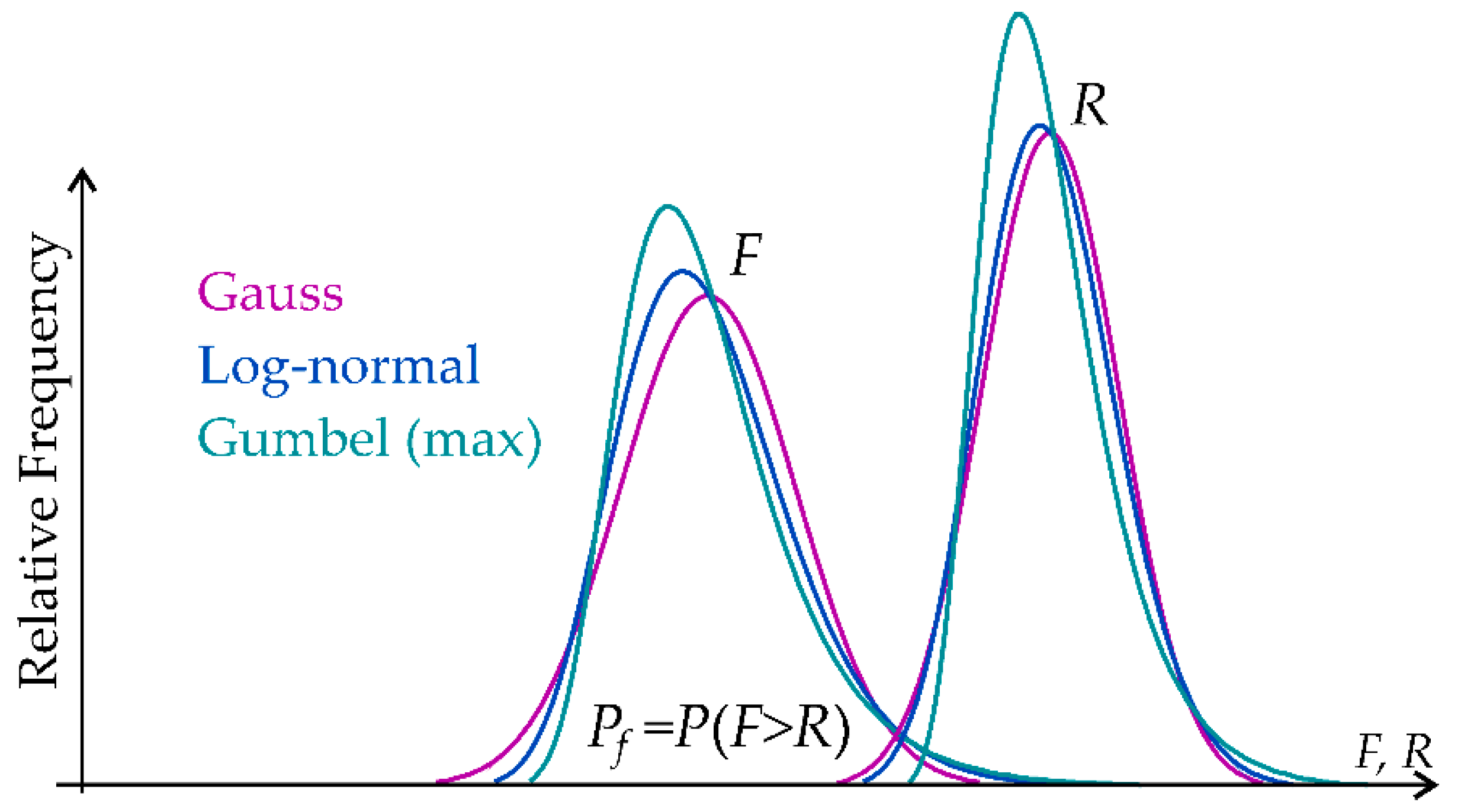
Figure 2.
Hermite fit to histograms: Histogram of yield strength with Gaussian baseline and Hermite fits: direct insertion of sample moments (red; rejected by KS) and refined inputs achieving moment matching (green; not rejected).
Figure 2.
Hermite fit to histograms: Histogram of yield strength with Gaussian baseline and Hermite fits: direct insertion of sample moments (red; rejected by KS) and refined inputs achieving moment matching (green; not rejected).
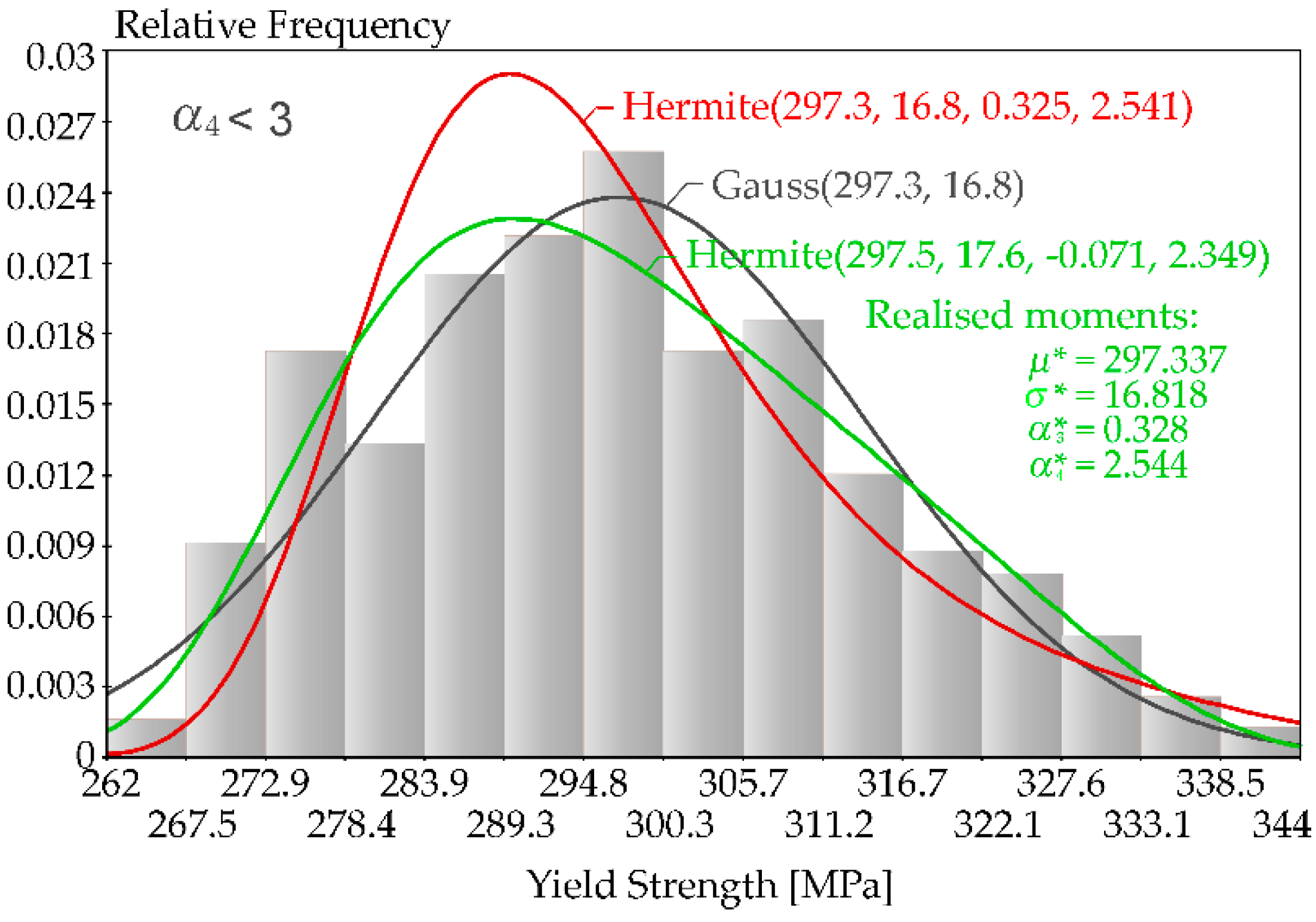
Figure 3.
Hermite fit to histograms: Histogram of ductility with Gaussian baseline and Hermite fits.
Figure 3.
Hermite fit to histograms: Histogram of ductility with Gaussian baseline and Hermite fits.
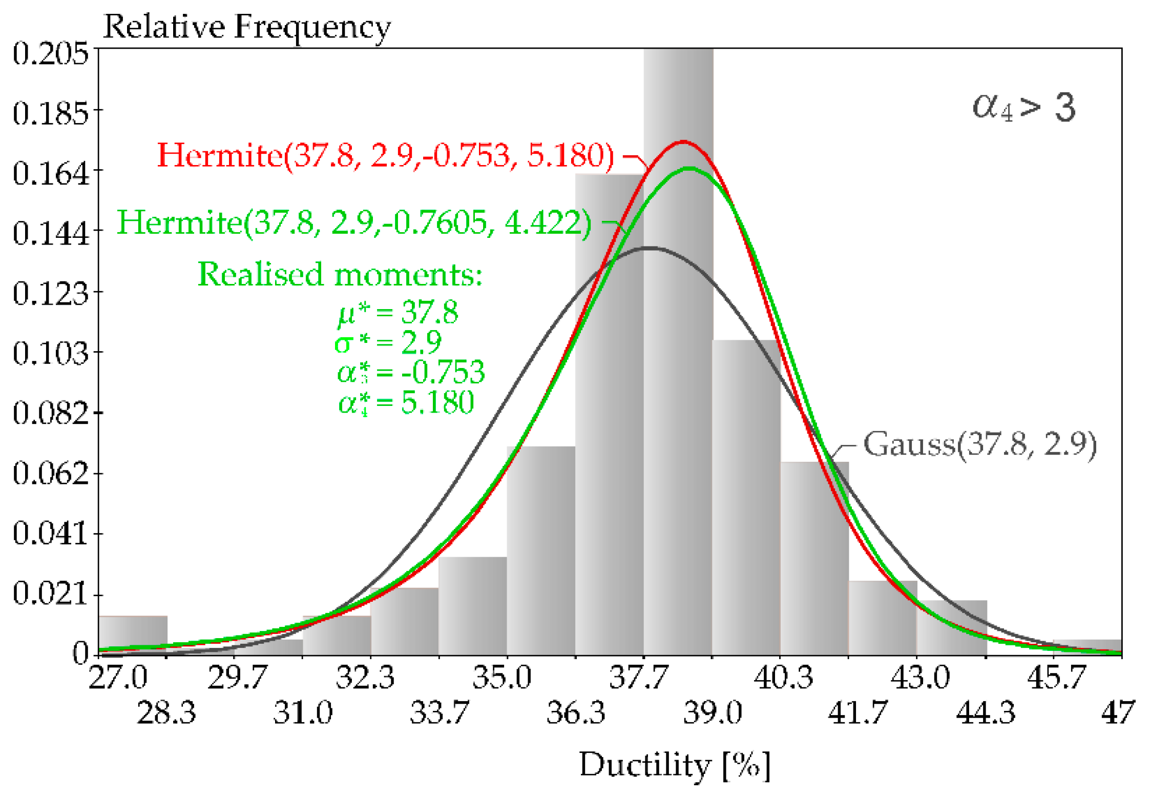
Figure 4.
Platykurtic branch (α4<3): illustrative Hermite pdfs under extreme-moment inputs.
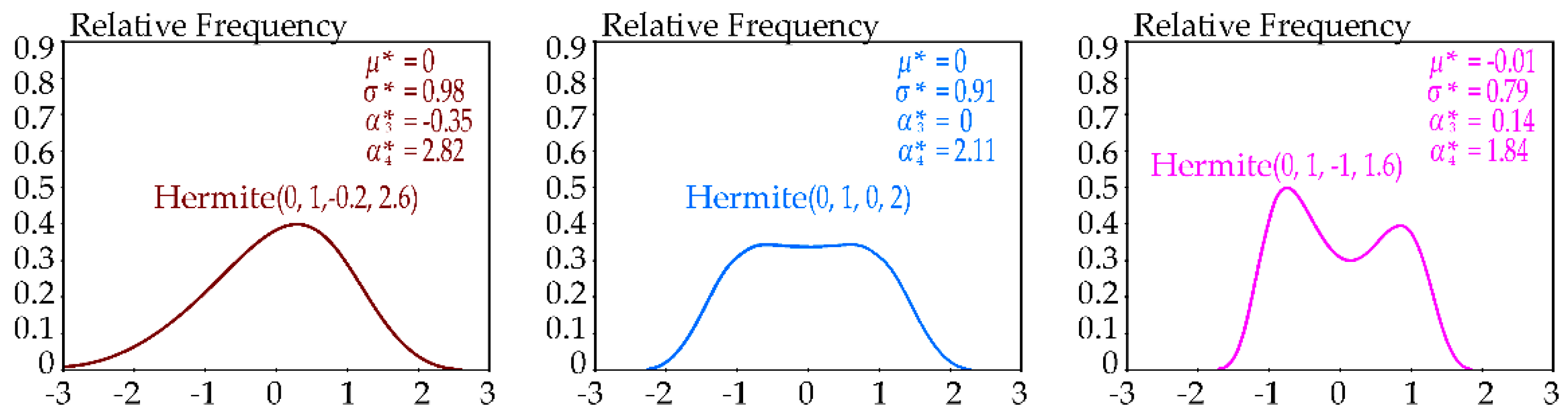
Figure 5.
Leptokurtic branch (α4>3): illustrative Hermite pdfs under extreme-moment inputs.
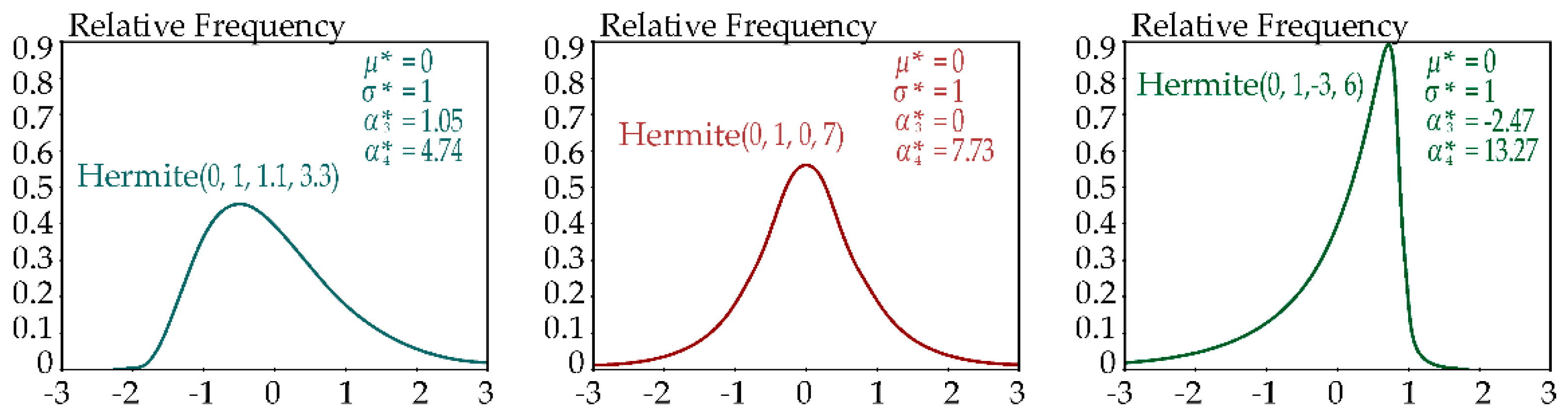
Figure 6.
Comparison of design quantiles Rd,HERM with Rd,FORM for βd=3.8.
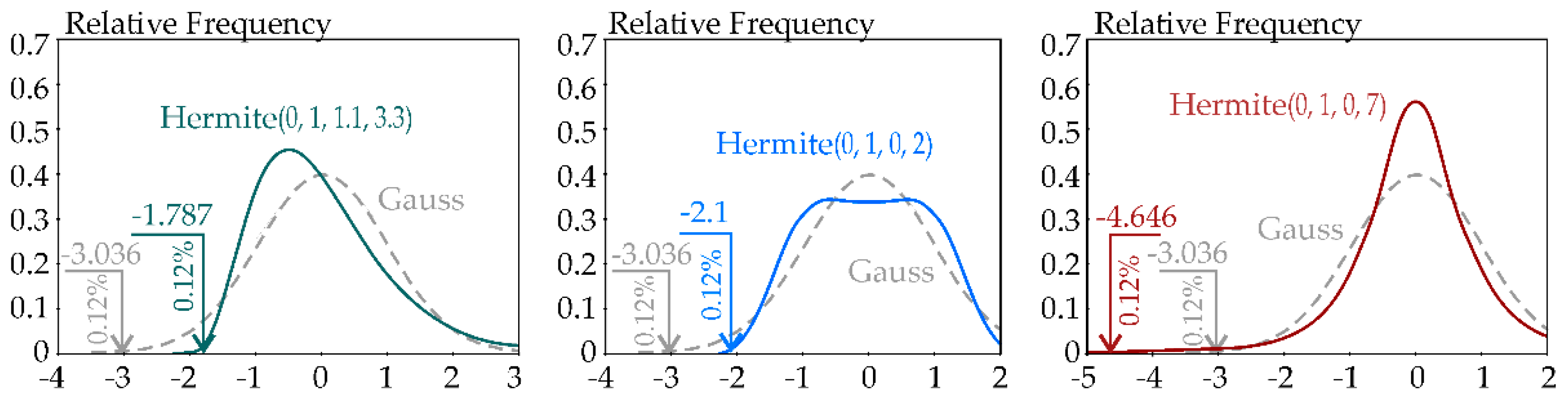
Figure 7.
Two pin-jointed bars with equilibrium of the internal forces F1 and F2 and external load F.
Figure 7.
Two pin-jointed bars with equilibrium of the internal forces F1 and F2 and external load F.
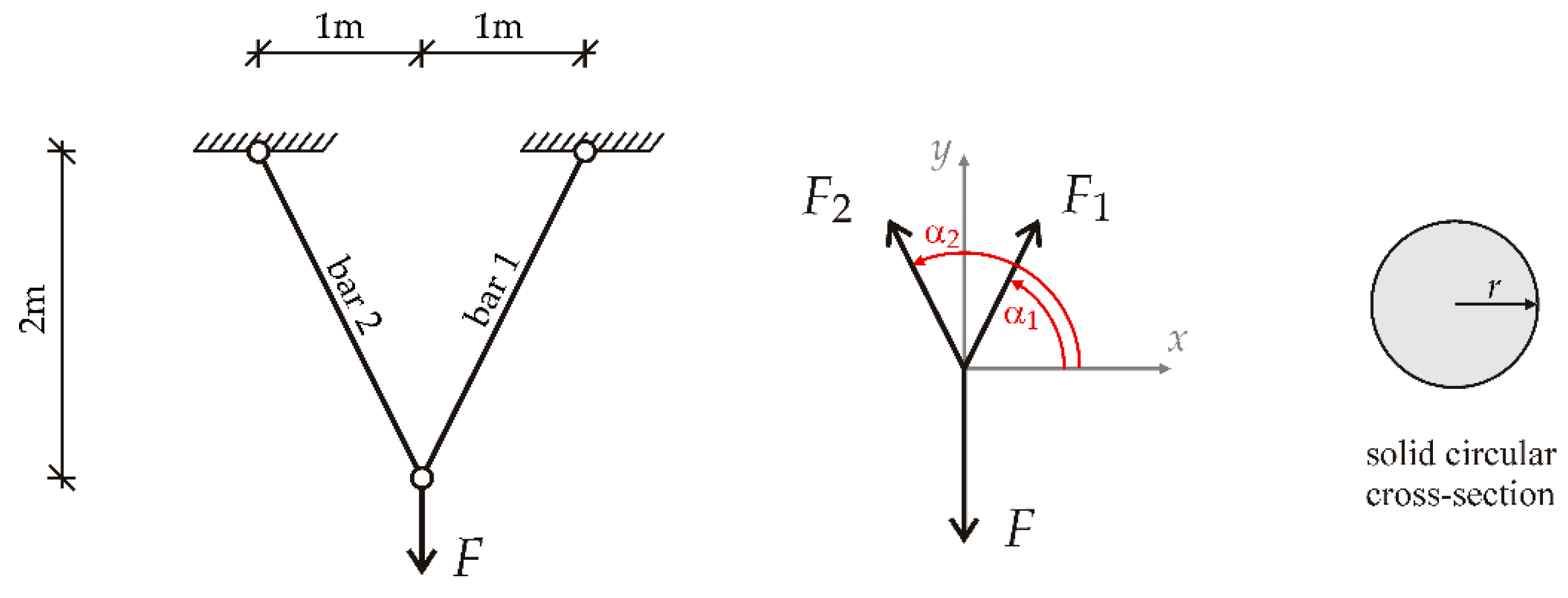
Figure 8.
Gaussian density of the input radius r and Sobol first-order and total sensitivity indices of the output resistance R.
Figure 8.
Gaussian density of the input radius r and Sobol first-order and total sensitivity indices of the output resistance R.
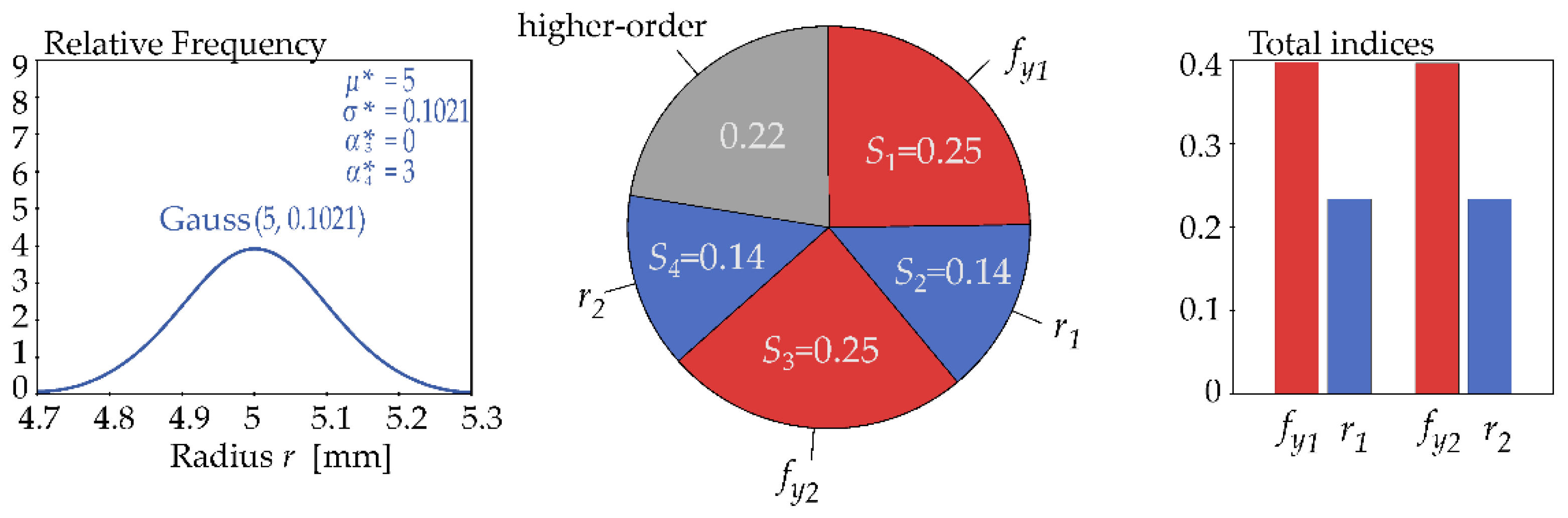
Figure 9.
Hermite density of the input radius r with negative skewness and elevated kurtosis and Sobol first-order and total sensitivity indices of the output resistance R.
Figure 9.
Hermite density of the input radius r with negative skewness and elevated kurtosis and Sobol first-order and total sensitivity indices of the output resistance R.
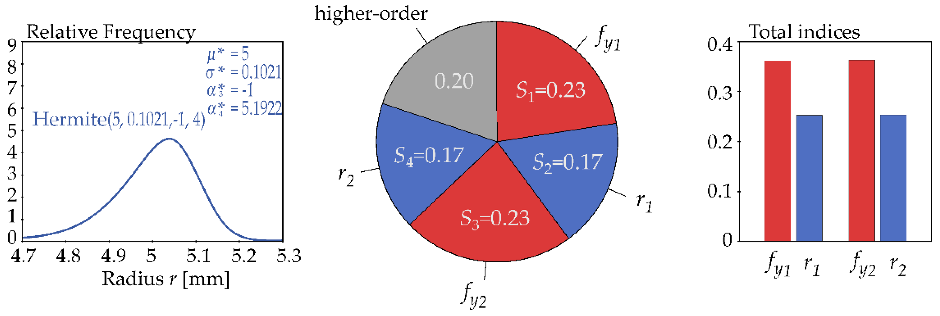
Figure 10.
Hermite density of the input radius r with stronger negative skewness and higher kurtosis and Sobol first-order and total sensitivity indices of the output resistance R.
Figure 10.
Hermite density of the input radius r with stronger negative skewness and higher kurtosis and Sobol first-order and total sensitivity indices of the output resistance R.
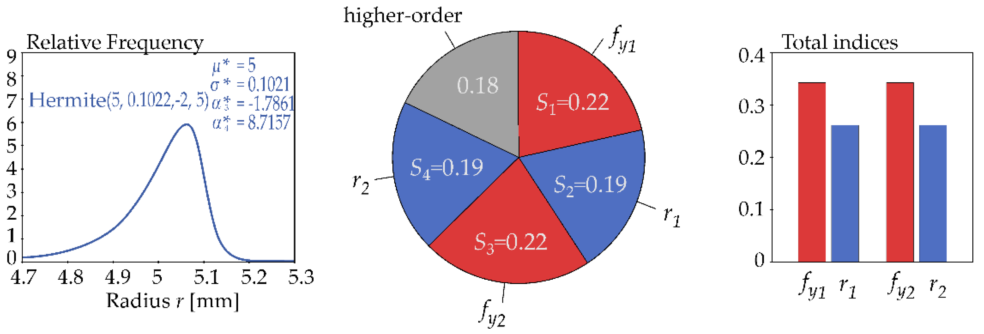
Figure 11.
Hermite density of the input radius r with pronounced negative skewness and markedly higher kurtosis and Sobol first-order and total sensitivity indices of the output resistance R.
Figure 11.
Hermite density of the input radius r with pronounced negative skewness and markedly higher kurtosis and Sobol first-order and total sensitivity indices of the output resistance R.
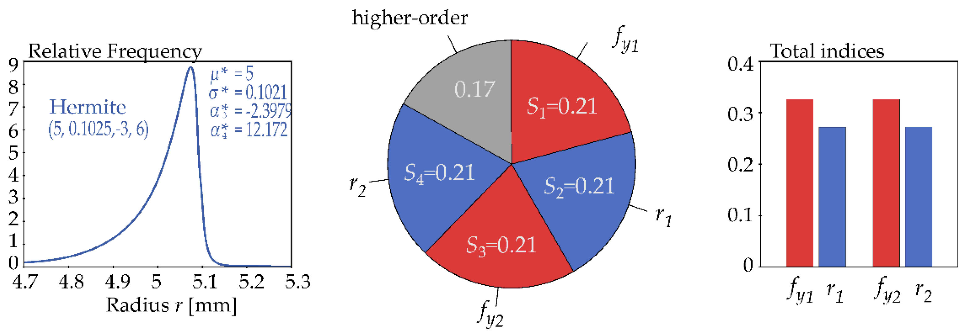
Figure 12.
Histogram and Monte Carlo Runs of the Resistance R for the Case (α3,r, α4,r)=(−3,6).
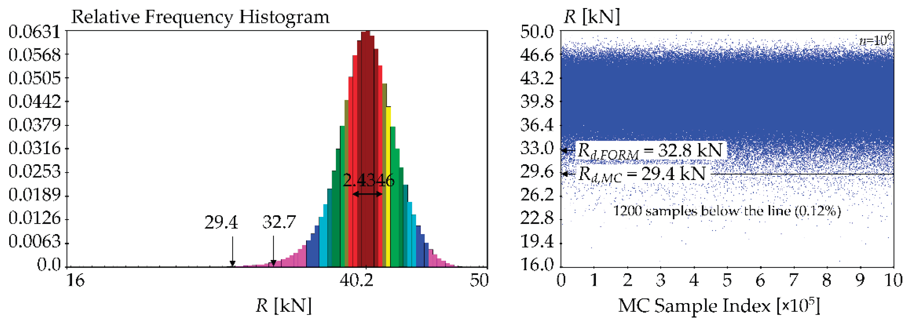

Table 1.
Input random quantities.
| Quantity | Density | ||||
| Yield strength fy1 | 297.5 | 17.6 | -0.071 | 2.349 | Hermite |
| Radius r1 | 5 | 0.1021 | Hermite | ||
| Yield strength fy2 | 297.5 | 17.6 | -0.071 | 2.349 | Hermite |
| Radius r2 | 5 | 0.1021 | Hermite |
The skewness and kurtosis of the radius ri are denoted by α3,r and α4,r. The parametric study fixes μr = 5 mm and σr = 0.1021 mm, while the pairs (α3,r, α4,r) = (0, 3), (−1, 4), (−2, 5), (−3, 6) are examined.
Table 2.
Output moments of R and design value Rd for Gaussian Hermite.
| Density of input radius r | [kN] | [kN] | [-] | [-] | Rd,FORM [kN] |
| Gauss(5, 0.1021) | 40.1431 | 2.2494 | 0.2161 | 3.0073 | 33.3048 |
| Hermite(5, 0.1021, -1, 4) | 40.1513 | 2.3351 | -0.0784 | 3.6834 | 33.0523 |
| Hermite(5, 0.1022, -2, 5) | 40.1611 | 2.4039 | -0.4209 | 5.9759 | 32.8532 |
| Hermite(5, 0.1025, -3, 6) | 40.1702 | 2.4539 | -0.6874 | 7.8546 | 32.7103 |
,,,denote moments of R evaluated by numerical integration with N=400.
Table 3.
Comparison of design quantiles of resistance R: Hermite closed form (Rd,HERM), numerical integration (Rd,HERM-INT), and FORM (Rd,FORM).
Table 3.
Comparison of design quantiles of resistance R: Hermite closed form (Rd,HERM), numerical integration (Rd,HERM-INT), and FORM (Rd,FORM).
| Density of output resistance R |
Rd,HERM-INT [kN] (n. integration) |
Rd,HERM [kN] Equation (47) |
Rd,FORM [kN] |
| Hermite(40.1443, 2.2517, 0.2051, 2.898) | 34.0463 | 34.2636 | 33.3048 |
| Hermite(40.1513, 2.3351, −0.0781, 3.6634) | 31.8476 | 31.8312 | 33.0523 |
| Hermite(40.1611, 2.4039, −0.4164, 5.5009) | 29.0760 | 29.0463 | 32.8532 |
| Hermite(40.1702, 2.4539, −0.6821, 6.7349) | 27.5294 | 27.4957 | 32.7103 |
Parameters of Hermite pdf are obtained using calibration of moments in Table 2. Rd,HERM-INT is calculated by numerical integration from the Hermite pdf.
Table 4.
Monte Carlo analysis of output statistics of R and design value Rd,FORM.
| Input model for radius r | [kN] | [kN] | [kN] | [kN] | Rd,FORM [kN] |
| Gauss(5, 0.1021) | 40.1388 | 2.2484 | 0.2158 | 3.0188 | 33.3037 |
| Hermite(5, 0.1021, -1, 4) | 40.1458 | 2.3343 | -0.0510 | 3.3672 | 33.0496 |
| Hermite(5, 0.1022, -2, 5) | 40.1583 | 2.3928 | -0.3085 | 3.9855 | 32.8843 |
| Hermite(5, 0.1025, -3, 6) | 40.1692 | 2.4346 | -0.5002 | 4.6400 | 32.7681 |
,,,denote moments of R evaluated by Monte Carlo method with n=1⋅106 runs.
Disclaimer/Publisher’s Note: The statements, opinions and data contained in all publications are solely those of the individual author(s) and contributor(s) and not of MDPI and/or the editor(s). MDPI and/or the editor(s) disclaim responsibility for any injury to people or property resulting from any ideas, methods, instructions or products referred to in the content. |
© 2025 by the authors. Licensee MDPI, Basel, Switzerland. This article is an open access article distributed under the terms and conditions of the Creative Commons Attribution (CC BY) license (http://creativecommons.org/licenses/by/4.0/).
Copyright: This open access article is published under a Creative Commons CC BY 4.0 license, which permit the free download, distribution, and reuse, provided that the author and preprint are cited in any reuse.


