
Submitted:
16 November 2025
Posted:
18 November 2025
You are already at the latest version
Abstract
Attention-Deficit/Hyperactivity Disorder (ADHD) is a prevalent neurodevelopmental disorder typically diagnosed through behavioral assessments and subjective reports. Electroencephalography (EEG) offers a cost-effective, non-invasive alternative for capturing neural activity patterns associated with the disorder. However, EEG-based ADHD classification remains challenged by overfitting, dependence on extensive preprocessing, and limited interpretability. Here, we propose T-GARNet, a novel neural architecture that integrates transformer-based temporal attention with Gaussian-mixture functional connectivity modeling and a cross-entropy loss regularized through α-Rényi mutual information. The multi-scale Gaussian kernel functional connectivity leverages parallel Gaussian kernels to identify complex spatial dependencies, which are further stabilized and regularized by the α-Rényi term. This design enables the direct modeling of long-range temporal dependencies from raw EEG while enhancing spatial interpretability and reducing feature redundancy. We evaluate T-GARNet on a publicly available ADHD EEG dataset using both leave-one-subject-out (LOSO) and stratified group k-fold cross-validation (SGKF-CV), where groups correspond to control and ADHD, and compare its performance against classical and modern state-of-the-art methods. Results show that T-GARNet achieves competitive or superior performance (88.3% accuracy), particularly under the more challenging SGKF-CV setting, while producing interpretable spatial attention patterns consistent with ADHD-related neurophysiological findings. These results underscore T-GARNet’s potential as a robust and explainable framework for objective EEG-based ADHD detection.
Keywords:
EEG
; ADHD
; Gaussian connectivity
; Rényi entropy
; neural networks
; transformer
1. Introduction
Attention-Deficit/Hyperactivity Disorder (ADHD) is a highly prevalent neurodevelopmental condition characterized by persistent patterns of inattention, hyperactivity, and impulsivity [1]. Globally, approximately 8% of children are affected [2], with continued symptomatology documented in up to two-thirds of diagnosed individuals into adulthood [3]. This persistence contributes to significant societal burdens, including reduced academic achievement and heightened demands on special education services [4]. Despite advances in diagnostic guidelines, current assessment procedures remain predominantly clinical, subjective, and highly dependent on trained practitioners, motivating a growing demand for objective, brain-based computational tools to support diagnosis [5].
Given ADHD’s strong association with brain function, neuroimaging techniques have gained attention as potential objective diagnostic aids. While functional magnetic resonance imaging (fMRI) has been employed, it poses challenges for pediatric populations due to motion sensitivity and high cost [6]. In contrast, electroencephalography (EEG) offers a portable, affordable, and non-invasive method to measure brain activity with high temporal resolution. The advent of deep learning has catalyzed the use of EEG for ADHD detection by offering a means to analyze its complex signals [7]. Deep learning models can identify subtle, high-dimensional patterns in EEG data that may elude traditional analysis, promising objective, scalable, and low-cost tools for early diagnosis [8].
However, translating these advances into clinically deployable tools remains challenging due to several fundamental barriers. A primary limitation is the conventional reliance on rigid, multi-stage EEG preprocessing pipelines. Such pipelines typically include filtering, artifact removal, frequency-band decomposition, and handcrafted feature extraction [9]. While designed to suppress noise and enforce domain priors, these stages rely on strong a-priori assumptions about neural activity. This approach risks the irreversible removal of potentially valuable information, such as subtle cross-frequency couplings or non-linear transient dynamics, thereby limiting the model’s ability to discover novel biomarkers from the full richness of the raw signal [10]. Besides, EEG signals exhibit substantial inter-subject variability, and ADHD itself presents heterogeneous neurocognitive profiles [11]. Models trained on limited or homogeneous cohorts frequently experience significant performance degradation when evaluated on new subjects or recording conditions, revealing vulnerability to domain shift and subject-specific noise [12]. This suggests that many existing approaches inadvertently learn dataset-specific artifacts rather than invariant neurophysiological structure [13].
In addition, a critical challenge is the tension between interpretability and expressive feature learning. Traditional machine learning approaches provide transparency but depend on predefined, handcrafted features that may overlook complex spatiotemporal mechanisms associated with ADHD [14]. Conversely, recent end-to-end deep learning models can learn rich representations directly from minimally filtered EEG [15], but often operate as opaque “black boxes.” This lack of neuroscientific interpretability complicates biomarker discovery, reduces clinical trust, and hinders the deployment of automated EEG-based ADHD assessment systems in medical settings [16].
Recently, EEG-based functional connectivity approaches have gained traction for their ability to capture coordinated neural activity across distributed brain regions [17]. Prior efforts have incorporated correlation matrices, coherence metrics, and graph theoretical measures into deep classifiers [18]. While promising, these methods frequently depend on exhaustive preprocessing or predefined frequency bands that constrain their representational flexibility [19]. Additionally, many existing works rely on evaluation strategies prone to information leakage, such as overlapping window segmentation without guaranteeing subject-level independence, limiting their clinical validity [20]. Besides, traditional EEG classification methods for ADHD typically rely on handcrafted feature extraction in time, frequency, or time-frequency domains. Techniques such as wavelet transforms, power spectral density estimation, entropy measures, and fractal dimension analysis have been extensively applied to capture oscillatory dynamics and non-linear behavior in EEG signals [21,22]. Among these, Common Spatial Patterns (CSP) remain a widely adopted approach due to their ability to enhance discriminative spatial filters between classes [23,24]. Despite their interpretability and relatively low computational cost, these methods heavily depend on extensive preprocessing and strong domain-specific priors. Moreover, many studies have been limited by suboptimal validation strategies, including within-subject cross-validation or overlapping window schemes, which compromise clinical generalization [25]. These limitations highlight the need for subject-independent evaluation protocols, such as leave-subject-out cross-validation, and the development of more flexible, data-driven feature extraction techniques [26].
In response to these challenges, deep learning has emerged as a powerful alternative, capable of learning hierarchical representations directly from minimally processed EEG data. Convolutional Neural Networks (CNNs) have been widely applied by transforming EEG signals into time–frequency maps or connectivity matrices [27,28]. Among these, EEGNet has become a benchmark architecture due to its compact design and its use of depthwise–separable temporal and spatial convolutions tailored for EEG analysis [29]. Building on this idea, several variants have been proposed from residual, fusion, and attention-based frameworks, which incorporate residual shortcuts, channel-wise attention, or frequency-adaptive modules to enhance expressive power [30,31].
Beyond EEGNet, earlier yet influential convolutional models such as ShallowConvNet and DeepConvNet [32] have demonstrated the effectiveness of hierarchical temporal–spatial filtering, with ShallowConvNet emphasizing band-power extraction and DeepConvNet enabling deeper abstraction of spectral–temporal patterns. More recent architectures adopt hybrid or modular designs—such as Temporal Convolutional Networks (TCN)-based models, Recurrent Neural Networks (RNN), RNN-CNN hybrids, Graph Convolutional Networks (GCNs) for functional connectivity, and spectral–temporal attention networks—to better capture long-range temporal dependencies, cross-channel interactions, and subject-specific variability [33,34,35]. However, despite their progress, many of these architectures remain limited in interpretability and continue to struggle with overfitting when trained on small or heterogeneous EEG datasets [36].
In turn, transformers have recently demonstrated strong performance in EEG analysis due to their ability to capture long-range temporal dependencies and learn attention maps interpretable as channel relevance patterns [37]. Nevertheless, their high modeling capacity also makes them particularly susceptible to overfitting in low-sample, high-variance EEG settings, where they may inadvertently learn subject-specific instead of neurophysiologically meaningful structure [38,39]. Meanwhile, information-theoretic regularization has shown strong potential to promote disentangled and complementary feature learning, particularly through Rényi entropy-based formulations that offer robust sensitivity to higher-order statistical structure [40]. Yet, this powerful mathematical framework remains underexplored in clinical EEG modeling.
To address these challenges, we introduce T-GARNet, a Transformer and Gaussian Mixture Connectivity Network with -Rényi regularization for EEG-based ADHD detection. T-GARNet jointly models temporal dynamics via a Transformer encoder and spatial structure via a Gaussian mixture connectivity module that learns latent interaction kernels across EEG channels without requiring predefined connectivity measures [41]. To further ensure the representation diversity essential for interpretability and generalization, we incorporate a mutual-information penalty based on -Rényi entropy that encourages complementary feature extraction across attention heads and connectivity kernels [42]. This principled framework enables direct learning from minimally preprocessed EEG, supports neuroscientific interpretability, and promotes robust out-of-distribution generalization. Namely, the main contributions of this work are as follows:
- –
- We propose a novel deep learning architecture that integrates Transformer-based temporal modeling with Gaussian mixture connectivity to learn spatiotemporal EEG representations without handcrafted features.
- –
- We introduce an -Rényi mutual-information regularizer that enforces representation diversity across attention and connectivity components, reducing redundancy and supporting interpretability.
- –
- We develop a multi-level interpretability scheme combining attention-based channel relevance, Gaussian kernel class activation maps, and structured ablation analysis to reveal neurophysiological patterns associated with ADHD.
- –
- We conduct extensive experiments using subject-group cross-validation and comparative baselines, demonstrating competitive performance and strong interpretability on a pediatric EEG ADHD dataset.
Overall, T-GARNet advances EEG-based ADHD detection by unifying principled information-theoretic regularization, connectivity-aware learning, and explainable attention mechanisms, providing a reliable and interpretable deep neural framework for pediatric neurodevelopmental assessment.
2. Materials and Methods
The proposed T-GARNet framework integrates mathematical principles from kernel information theory with modern deep sequence modeling to extract interpretable spatio-temporal connectivity patterns from EEG signals. This section presents the theoretical foundations, followed by the model architecture and the associated optimization scheme.
2.1. Kernel Methods and Functional Mapping
Kernel methods provide a powerful strategy for capturing nonlinear relationships by implicitly mapping data into a high-dimensional reproducing kernel Hilbert space (RKHS). Let denote the input domain. A kernel function defines an inner product in an RKHS via , where is an implicit feature map [43]. This bypasses the need to compute explicitly, enabling the analysis of complex dependencies via pairwise similarities.
2.2. Matrix-Based -Rényi Entropy and Mutual Information
Let X be a continuous random variable defined on with probability density function (PDF) . The -Rényi entropy for and , is defined as:
Since is generally unknown in high-dimensional settings, it may be approximated via kernel density estimation (KDE) using N i.i.d. samples :
where denotes a Gaussian kernel as in equation 1.
For , Rényi entropy reduces to quadratic entropy, linked to the Information Potential (IP) [46]:
Now, let be a Gram matrix with entries . Then
where is the all-ones vector. Next, define a normalized matrix if gathers its eigenvalues; the matrix-based -Rényi entropy becomes [47]:
For the quadratic case , a numerically stable formulation is
Next, let X and Y denote random variables with kernel matrices and . Their joint kernel is computed via the Hadamard product:
and its normalized version yields the joint entropy:
The matrix-based mutual information (MI) follows:
This formulation offers three advantages crucial for EEG modeling:
- –
- Nonparametric: no assumptions on the underlying EEG distribution.
- –
- Differentiable: allows end-to-end learning with backpropagation.
- –
- Redundancy control: high MI between kernel-induced representations is penalized, encouraging disentangled connectivity patterns across spatial scales.
In T-GARNet, this mutual information regularizer ensures that multi-scale Gaussian connectivity matrices do not learn overlapping neural relationships, promoting complementary and interpretable spatial structure while reducing model overfitting.
2.3. Multi-Scale Gaussian Kernel Connectivity
Functional connectivity in EEG reflects coordinated neural activity across cortical regions. To represent such interactions in a principled and data–driven manner, we construct kernel–based similarity matrices between channels. This formulation is grounded in the spectral properties of stationary stochastic processes and their correspondence with positive–definite kernels.
Let be a wide-sense stationary process with autocorrelation function:
where is an absolutely continuous spectral distribution and denotes its power spectral density [48]. Thus, second–order temporal statistics are fully characterized by a spectral measure. A key theoretical foundation comes from Bochner’s theorem, which states that a continuous function is stationary and positive–definite if and only if it admits a spectral representation:
for some finite, non–negative measure . This result establishes a direct equivalence between valid kernels and valid spectral distributions. In practical terms, a kernel implicitly defines a spectral density, making kernel matrices a natural surrogate for neurophysiological connectivity patterns [41].
For multichannel EEG signals , this interpretation extends to a cross–spectral representation:
where denotes the cross–spectral density and its cumulative distribution. Therefore, kernel similarity between two channels implicitly reflects a frequency–dependent interaction profile.
Of note, direct estimation of in EEG is notoriously challenging due to noise, limited data, and nonstationarity. A widely used surrogate is to approximate the spectral distribution with a Gaussian function, as in equation 1. The bandwidth controls spatial scale: smaller values emphasize local, fine–grained connectivity, while larger values capture distributed interactions across the cortex.
To account for the multi-scale nature of brain networks, we construct a convex mixture of G Gaussian kernels, as follows:
where is the kernel matrix associated with scale and are learnable mixture coefficients. This generates a multi–resolution connectivity representation while ensuring positivity and proper normalization.
Within the proposed T-GARNet, these kernel matrices provide structured spatial representations of the EEG that complement the temporal dependencies learned by the Transformer encoder. Each kernel captures connectivity at a distinct cortical scale, and the convex combination allows the network to adaptively integrate local and global synchrony patterns relevant to ADHD. These connectivity maps are subsequently processed by convolutional layers, enabling hierarchical refinement and interaction between spatial patterns. Combined with the –Rényi regularization term, the framework encourages complementary connectivity features across scales, improving interpretability and robustness.
2.4. Transformer and Multi-Kernel Gaussian Connectivity Network with -Rényi Regularization
Let denote an EEG trial with C channels and T temporal samples. Each segment is first transposed to , treating each time step as a token with a C-dimensional feature representation. this tokenization aligns with Transformer-based modeling of sequential biomedical signals, enabling the extraction of long-range temporal dependencies while preserving spatial structure across electrodes.
The token sequence is processed by a single Transformer encoder block composed of multi-head self-attention (MHSA) and a positionwise feedforward network. For each attention head , the input matrix is linearly projected into Queries (), Keys (), and Values ():
where the weight matrices and are learnable parameters. In the canonical setting, .
The attention output of head h is computed as:
The MHSA operation concatenates all heads and projects them back to :
where is a learned output projection matrix. This mechanism learns scale-adaptive temporal dependencies across EEG tokens, while the attention weights provide physiologically interpretable channel relevance cues.
The MHSA output is passed through a positionwise MLP with residual connections and layer normalization, following standard Transformer design (see Figure 1) [49]. The resulting representation: encodes temporal dependencies enriched by channel–wise contributions.
Also, the temporal representation produced by the Transformer encoder is transposed to so that each row corresponds to a channel-level feature vector. From this representation, we compute a bank of G Gaussian kernel connectivity matrices that integrate information across resolutions; the kernel bank is combined through a learned convex mixture:
producing a single multi-scale connectivity matrix. The coefficients are trainable attention-like weights that adaptively emphasize the most informative spatial resolutions.
is refined through two convolution–normalization blocks. Formally,
where each convolution uses small spatial kernels to enhance localized EEG interactions. Afterward, the obtained representation is vectorized and classified via a dense layer:
where denotes the predicted probabilities for ADHD and control classes.
Our T-GARNet loss combines normalized binary cross-entropy with an information–theoretic term that penalizes redundancy across the G multi–scale connectivity matrices. First, the Normalized Binary Cross-Entropy, yields:
where is the batch size, the ground-truth label, and the predicted probability for the positive class. Second, an -Rényi mutual-information across kernel scales is employed. Namely, let be the Gaussian connectivity matrices and define their trace-normalized versions . Denote by the matrix-based -Rényi entropy. Then, our MI loss over scales is defined as follows:
This term is minimized when the joint entropy of the Hadamard aggregation approaches the sum of marginal entropies, encouraging complementary (non-redundant) information across spatial scales. Consequently, the T-GARNet total loss is written as:
Figure 2 summarizes the core components and training pipeline of our proposed T-GARNet model for ADHD detection.
3. Experimental Set-Up
3.1. Tested ADHD Dataset
This study uses an EEG dataset publicly available on IEEE DataPort [50], comprising recordings from 121 children aged 7 to 12 years, including 61 with ADHD and 60 healthy controls (accessed on 1 July 2025). ADHD diagnoses were made by an experienced psychiatrist following DSM-IV criteria, and participants had received Ritalin treatment for no longer than six months. Control subjects had no history of psychiatric or neurological conditions. A summary of participant demographics and EEG acquisition parameters is presented in Table 1.
EEG data were recorded using the 10–20 system with 19 electrodes and referenced to A1 and A2 on the earlobes (see Figure 3a), sampled at 128 Hz. The recording protocol was designed to assess visual attention, a cognitive function often impaired in children with ADHD. During the task, children viewed cartoon images and were asked to count the number of characters (randomly 5–16 per image). Stimuli were presented in rapid succession immediately following each response, making total recording duration dependent on individual response speed (see Figure 3b).
To ensure class balance prior to model training, one ADHD subject was randomly removed from the dataset, resulting in a final sample of 120 participants (60 control and 60 ADHD). After balancing, all subsequent analyses proceeded as described. To minimize preprocessing bias and evaluate the model’s capacity to learn directly from raw electrophysiological structure, EEG signals were fed to the network without artifact removal, filtering, or spectral band decomposition. This design enables the model to operate on minimally processed neural activity, avoiding conventional assumptions about spectral relevance and reducing the risk of discarding physiologically meaningful dynamics. Also, following standard practice in EEG-based classification [19], recordings were segmented into 4-second epochs (512 samples at 128 Hz) with a 50% overlap. Consecutive windows therefore begin every 2 seconds, yielding dense temporal sampling while preserving temporal independence assumptions (see Figure 4). This segmentation produced: Control group: 3,657 segments (mean per subject) and ADHD group: 4,622 segments (mean per subject). Moreover, each epoch was treated as an independent training instance, but subject identity was preserved and never mixed across folds, ensuring strict subject-wise separation in all evaluation pipelines.
3.2. Assessment, Model Comparison, and Training Details
To assess generalization under rigorous subject-independent conditions, two complementary validation schemes were implemented (refer to the illustrative example in which two distinct validation methodologies are juxtaposed with Holdout validation, as depicted in Figure 5).
- –
- Leave-One-Subject-Out Cross-Validation (LOSO-CV). At each iteration, data from a single subject were held out exclusively for testing, while the remaining subjects formed the training set. This is repeated N times so that each participant serves as the test set once.
- –
- Stratified Group k-Fold Cross-Validation (SGKF-CV). A subject-wise stratified k-fold scheme () was employed. For each fold, 24 subjects (12 ADHD, 12 controls) were reserved for testing, and the remaining 96 subjects formed the training set. Stratification maintained class balance across folds.
In both protocols, no temporal or subject-level data leakage occurred. Segments from the same subject never appeared in both training and testing sets.
T-GARNet was benchmarked against five baseline models selected to represent complementary design paradigms in EEG learning. The objective was to position the proposed architecture within a broad methodological landscape, spanning traditional machine learning, compact convolutional models, recurrent hybrids, and Transformer-based systems. The reference models included:
- –
- CNN-based Architectures (ShallowConvNet [32], EEGNet [29]): These models represent compact, efficient, and widely adopted CNNs designed specifically for end-to-end EEG processing. They serve as a baseline to evaluate the performance of standard deep learning approaches that do not explicitly model connectivity or long-range temporal dependencies with attention.
- –
- Hybrid Architecture (CNN-LSTM [33]): This model combines CNNs with recurrent neural networks (LSTMs). It provides a point of comparison for evaluating T-GARNet’s Transformer-based approach against more traditional methods for modeling temporal sequences.
- –
- Attention-based Architecture (Multi-Stream Transformer [19]): This model also uses Transformers, but processes spectral, spatial, and temporal streams independently. It serves as a critical baseline to evaluate the benefits of T-GARNet’s integrated architecture, where temporal attention and spatial connectivity modeling are directly linked.
- –
- Classical Machine Learning Pipeline (ANOVA-PCA SVM [38]): This model represents a traditional, non-end-to-end approach involving explicit feature engineering, selection, and classification. It provides a baseline to quantify the performance gains achieved by deep learning methodologies.
All networks were trained and evaluated using identical cross-validation folds to enable direct comparison. In keeping with the original methodological prescriptions, preprocessing was applied only to the models that explicitly require it (ANOVA–PCA SVM and Multi-Stream Transformer). Deep learning models that support raw EEG input, including T-GARNet, were evaluated on minimally processed signals to preserve comparability in end-to-end settings. Table 2 summarizes the architectural components, parameter counts, and the model ability to operate directly on raw EEG.
Deep learning models were trained using the Adam optimizer with a batch size of 16 and a maximum of 150 epochs. Training employed two stabilization strategies to balance convergence and generalization: early stopping halted optimization when the validation loss failed to improve by over 25 consecutive epochs, restoring the best-performing weights, and a ReduceLROnPlateau scheduler decreased the learning rate by a factor of 0.5 after 10 stagnant epochs, with a floor of . The latter allows progressive refinement in later training stages while mitigating overfitting and premature convergence.
All experiments were executed in a cloud-based Kaggle environment using Python 3.11.11 and TensorFlow 2.18.0. The hardware configuration included an Intel Xeon CPU @ 2.00 GHz (4 logical cores), 31 GB RAM, and two NVIDIA Tesla T4 GPUs with 15 GB VRAM each, operating under a 64-bit Ubuntu-based system. GPU acceleration was enabled through CUDA 12.6 and NVIDIA driver version 560.35.03. For reproducibility, all source code, scripts, and configuration files are available online at https://github.com/dannasalazar11/Msc_thesis/tree/main/TGARNet.
4. Results and Discussion
This section reports the performance of the proposed T-GARNet model under two complementary subject–independent validation schemes: SGKF–CV and LOSO-CV. These protocols assess model robustness to inter–subject variability and acquisition heterogeneity, which are critical for the development of clinically reliable EEG–based diagnostic systems. In addition to classification performance, we evaluate the contribution of the proposed multi–scale Gaussian connectivity module and the –Rényi mutual information regularization in enabling interpretable and non–redundant spatial representations.
Performance was quantified using standard binary–classification metrics computed at the segment level. Let , , , and denote true positives, true negatives, false positives, and false negatives. We report:
All metrics were averaged across folds, and standard deviations were computed to quantify performance variability across subjects.
4.1. Performance Under the LOSO–CV Protocol
Table 3 presents the performance of all models under the LOSO evaluation protocol. Consistent with prior ADHD EEG studies employing subject–wise validation, all end–to–end deep learning architectures achieve high precision, with EEGNet and CNN–LSTM leading, closely followed by T-GARNet and ShallowConvNet. This convergence toward ceiling–level performance reflects the well–known behavior of LOSO in small to medium EEG datasets, where overlapping temporal windows from the same subject preserve individual–specific spectral–temporal fingerprints across folds.
Under these favorable conditions, T-GARNet demonstrates competitive performance, achieving precision comparable to top baselines. This confirms that the addition of multi–scale Gaussian connectivity modeling and –Rényi regularization does not impede discriminative capacity when subject–specific signal structure is implicitly shared across training and test partitions. Moreover, the variance pattern across architectures follows expected trends: models relying heavily on global attention exhibit greater variability, reflecting sensitivity to subject–specific noise, whereas T-GARNet preserves stability by enforcing spatial structure and information–diversity constraints.
Overall, while LOSO does not fully expose differences in generalization behavior due to its optimistic bias, T-GARNet remains on par with leading deep learning baselines. This motivates the complementary use of the SGKF–CV protocol, which enforces separation across subject groups and provides a more realistic estimate of out–of–distribution clinical performance.
4.2. Performance Under the SGKF–CV Protocol
To obtain a more realistic estimate of clinical generalization, we performed a stratified group k–fold cross–validation, where entire groups of subjects were held out in each fold. This protocol enforces subject–level independence while avoiding optimistic bias that may arise in LOSO settings due to segment overlap and subject–specific patterns. Unlike LOSO, SGKF–CV evaluates whether the model can generalize to larger unseen cohorts, closely reflecting deployment scenarios where new patients exhibit distinct noise characteristics and individual neurophysiological variability.
Table 4 reports the average performance across folds. T-GARNet achieves the highest mean accuracy and recall among all evaluated architectures, outperforming compact convolutional models (ShallowConvNet, EEGNet), recurrent hybrids (CNN–LSTM), and both transformer and classical pipelines. The improvement is most pronounced relative to the Multi–Stream Transformer and ANOVA–PCA SVM, highlighting the importance of jointly learning temporal dependencies and functional connectivity representations rather than decoupling them or relying on handcrafted features.
The elevated recall reflects T-GARNet’s superior ability to correctly detect ADHD segments, a clinically important characteristic given the consequences of underdiagnosis. Notably, this sensitivity is achieved without sacrificing precision, indicating that the model does not inflate false positives. These effects are visually supported by the confusion matrices in Figure 6, where T-GARNet exhibits the most balanced error distribution and lowest misclassification rates between ADHD and control segments.
4.3. Statistical Significance Analysis
To assess whether performance differences among models were statistically meaningful, a Friedman test followed by Wilcoxon signed–rank post–hoc analysis with Holm correction was conducted [51]. Results were computed from 50 accuracy values per model (5 folds × 10 repetitions).
The Friedman test indicated significant differences across classifiers (, ), confirming that the choice of model has a measurable effect on classification accuracy. Table 5 summarizes the average ranking, win frequency, and post–hoc comparisons.
T-GARNet achieved the best average rank (2.28) and the highest number of fold wins (19/50), indicating consistently strong performance. Post–hoc Holm–corrected Wilcoxon tests showed that T-GARNet significantly outperformed the Multi-Stream Transformer and the ANOVA-PCA SVM (). Differences with EEGNet, CNN-LSTM, and ShallowConvNet were not statistically significant after correction, reflecting the competitive nature of these strong baselines.
These results demonstrate that T-GARNet matches or exceeds state-of-the-art performance while providing improved interpretability through its attention-guided kernel connectivity and information-theoretic regularization.
4.4. Transformer-Based Channel Importance Analysis
To investigate the spatial contributions learned by the Transformer encoder, we analyzed the attention projection weights extracted from the trained T-GARNet model. Following the formulation introduced in Equation 15, these tensors represent channel-wise projections across H attention heads and embedding dimension d.
For each head h, we computed an inter-channel interaction matrix [52]:
which measures how strongly each EEG channel queries information from others. Averaging across all heads yields:
The column-wise -norm of defines the attention importance vector, reflecting how often each channel is consulted:
To incorporate the magnitude of the value projections, the overall content importance is computed as
yielding a normalized distribution of channel relevance across the EEG montage. This metric effectively combines how much a channel is queried (attentional demand) and how much information it contributes (content strength).
Figure 7 summarizes the channel-level importance scores across folds. Consistently across runs, the highest weights concentrate on midline and parietal electrodes (C4, P4, and P3), followed by prefrontal regions (Fp1/Fp2), reflecting the engagement of fronto-parietal control circuits often implicated in ADHD neurodynamics. Channels located in posterior and temporal areas exhibit comparatively lower weights, suggesting limited direct contribution to the temporal encoding learned by the Transformer.
To quantitatively assess the functional relevance of these learned importance scores, we performed a channel ablation experiment. Channels were progressively deactivated (set to zero) following two schemes: (1) ranked order according to , and (2) random order, averaged over 50 repetitions. Figure 8 shows the resulting mean accuracy drop as channels were removed. The ranked ablation curve declines sharply compared to the random baseline, indicating that early removal of the most important channels significantly degrades classification accuracy.
A two-sample t-test between the ranked and random ablations for the first five removals yielded a statistically significant difference (), confirming that the Transformer-identified channels encode discriminative information critical for the ADHD - control distinction.
4.5. Learned Connectivity Patterns
To gain insight into the neurophysiological representations captured by the proposed model, we analyzed the Gaussian–kernel connectivity matrix produced by the intermediate layer of T-GARNet. This matrix encodes pairwise channel interactions learned directly from raw EEG, allowing us to examine emergent connectivity patterns without imposing predefined frequency bands or handcrafted connectivity metrics.
For interpretability analysis, we selected the trained model from the fifth SGKF fold and extracted connectivity representations for two subjects in the held–out test group: one ADHD subject and one control subject. For each individual, connectivity matrices were computed for all EEG segments and then averaged across segments to obtain a stable subject–level connectivity map.
Figure 9 illustrates these averaged connectivity graphs. Each chord represents a learned functional interaction between EEG channels, with line thickness and color indicating kernel magnitude and thus the strength of modeled coupling.
Qualitative differences are apparent between the groups. The control subject exhibits a more localized and structured connectivity architecture, with short–range frontal and temporal interactions dominating the pattern. In contrast, the ADHD subject shows broader and more diffuse connectivity, including pronounced long–range interhemispheric and fronto–parietal couplings.
These connectivity signatures align with prior evidence of atypical large–scale communication and reduced network efficiency in ADHD, particularly in circuits associated with executive control and attentional regulation. Notably, such patterns emerged without explicit functional connectivity priors, suggesting that the proposed multi–scale Gaussian kernel mechanism learns clinically relevant coupling structures in a data–driven manner. Combined with the competitive classification performance, these results highlight the potential of T-GARNet as both a diagnostic tool and a model capable of revealing mechanistic neural alterations in ADHD.
4.6. Class–Wise Spatial Relevance via Grad-CAM++
To further inspect the spatial representations learned by T-GARNet, we computed class-specific activation maps (CAMs) from the last convolutional layer using the Grad-CAM++ implementation provided by keras-vis. For interpretability and to avoid information leakage, CAMs were calculated exclusively over the held-out test subjects from the SGKF-CV fold where Fold 5 served as the test partition.
For each test trial, a CAM was extracted, and the maps were then averaged separately across ADHD and Control samples:
To derive a channel-level relevance score, each CAM was collapsed across time:
Because the absolute magnitudes of these vectors may differ across classes, both relevance vectors were jointly normalized using their shared minimum and maximum:
with
Finally, the class-wise discriminative magnitude was computed as
highlighting channels whose relevance differs most between classes.
Figure 10 depicts the resulting topographies. The ADHD map (left) shows a frontal midline depression centered on Fz and pronounced posterior relevance with a right-occipital peak around O2, accompanied by contributions in P4/T6 and a secondary lobe near T5. The Control map (middle) exhibits an even deeper valley along the midline (Fz through Cz–Pz) and comparatively elevated lateral activity, yielding a more symmetric peripheral profile. The class-wise difference (right) highlights where the model’s spatial evidence diverges most: the strongest separations occur over fronto–lateral sites (F3/F4) and lateral central electrodes (C3/C4), whereas differences are minimal along the midline axis (Fz–Cz–Pz) and at occipital sites (O1/O2), where both classes show similar levels after joint normalization.
Overall, these CAM-derived patterns show that discrimination emerges primarily from lateral frontal (F3/F4) and central sensorimotor regions (C3/C4), whereas midline activity (Fz–Cz–Pz) remains largely shared between ADHD and control subjects, and occipital contributions are comparably low in both groups. This spatial distribution is consistent with neurophysiological evidence reporting that ADHD-related alterations during sustained attention tasks arise mainly in lateral prefrontal and sensorimotor circuits, rather than in midline executive regions whose engagement is driven by the task demands itself. The observed CAM differences therefore align well with established findings and reinforce a coherent interpretation in which lateral fronto–central dynamics encode most of the class-specific information, while midline and posterior activity reflect common processing across groups.
5. Conclusions
In this work, we introduced T-GARNet, a novel architecture that integrates Transformer-based temporal modeling with a multi-scale Gaussian kernel connectivity module regularized through matrix-based -Rényi mutual information. The model was designed to address three persistent challenges in EEG-based ADHD detection: the dependence on extensive preprocessing pipelines, limited interpretability of deep neural models, and poor generalization under subject-independent evaluation. Across two rigorous validation schemes, LOSO-CV and SGKF-CV, T-GARNet achieved competitive or superior performance relative to widely used convolutional, recurrent, and Transformer-based baselines. Notably, under the more clinically realistic SGKF-CV setting, the proposed framework demonstrated the highest average accuracy and recall while maintaining balanced precision, underscoring its robustness to inter-subject variability and acquisition heterogeneity.
Beyond classification accuracy, T-GARNet provided enhanced interpretability through multiple complementary mechanisms. The Transformer encoder produced channel-attention patterns that consistently emphasized fronto-central and parietal regions implicated in ADHD neurophysiology. The multi-scale Gaussian connectivity module revealed group-specific functional interactions without relying on handcrafted features or predefined frequency bands. Furthermore, the -Rényi regularization successfully encouraged diversity across connectivity scales, reducing redundancy and enabling clearer spatial structure. Grad-CAM++ analyses further confirmed class-discriminative relevance in lateral prefrontal and sensorimotor regions known to support attentional control. Taken together, these findings demonstrate that T-GARNet offers a principled and interpretable framework for EEG-based ADHD assessment. By jointly modeling temporal dependencies and connectivity structure while enforcing information-theoretic diversity, the model captures meaningful neurophysiological patterns directly from minimally processed EEG.
Author Contributions
Conceptualization, D.V.S.-D., A.A.-M. and G.C.-D.; data curation, D.V.S.-D.; methodology, D.V.S.-D., A.A.-M. and G.C.-D.; project administration, A.A.-M. and G.C.-D.; supervision, A.A.-M. and G.C.-D.; resources, D.V.S.-D. and A.A.-M.. All authors have read and agreed to the published version of the manuscript.
Funding
Authors gratefully acknowledge support from the program: “Alianza científica con enfoque comunitario para mitigar brechas de atención y manejo de trastornos mentales relacionados con impulsividad en Colombia (ACEMATE)-91908.” This research was supported by the project: “Sistema multimodal apoyado en juegos serios orientado a la evaluación e intervención neurocognitiva personalizada en trastornos de impulsividad asociados a TDAH como soporte a la intervención presencial y remota en entornos clínicos, educativos y comunitarios-790-2023,” funded by the Colombian Ministry of Science, Technology and Innovation (Minciencias). Also, A.M. Alvarez thanks to the project: "Aprendizaje de máquina cuántico utilizando espines electrónicos", Hermes-62836, funded by Universidad Nacional de Colombia and Universidad de Caldas.
Data Availability Statement
The databases and codes used in this study are public and can be found at the following link: https://github.com/dannasalazar11/Msc_thesis/tree/main/TGARNet (accessed on 1 July 2025).
References
- Asherson, P. ADHD across the lifespan. Medicine 2024, 52, 512–517. [Google Scholar] [CrossRef]
- Ayano, G.; Demelash, S.; Gizachew, Y.; Tsegay, L.; Alati, R. The global prevalence of attention deficit hyperactivity disorder in children and adolescents: An umbrella review of meta-analyses. Journal of affective disorders 2023, 339, 860–866. [Google Scholar] [CrossRef]
- Di Lorenzo, R.; Balducci, J.; Poppi, C.; Arcolin, E.; Cutino, A.; Ferri, P.; D’Amico, R.; Filippini, T. Children and adolescents with ADHD followed up to adulthood: A systematic review of long-term outcomes. Acta Neuropsychiatrica 2021, 33, 283–298. [Google Scholar] [CrossRef]
- van der Plas, N.E.; Noordermeer, S.D.; Oosterlaan, J.; Luman, M. Systematic Review and Meta-Analysis: Predictors of Adult Psychiatric Outcomes of Childhood Attention-Deficit/Hyperactivity Disorder. Journal of the American Academy of Child & Adolescent Psychiatry, 2025. [Google Scholar]
- Hurjui, I.A.; Hurjui, R.M.; Hurjui, L.L.; Serban, I.L.; Dobrin, I.; Apostu, M.; Dobrin, R.P. Biomarkers and Neuropsychological Tools in Attention-Deficit/Hyperactivity Disorder: From Subjectivity to Precision Diagnosis. Medicina 2025, 61, 1211. [Google Scholar] [CrossRef]
- Güven, A.; Altınkaynak, M.; Dolu, N.; İzzetoğlu, M.; Pektaş, F.; Özmen, S.; Demirci, E.; Batbat, T. Combining functional near-infrared spectroscopy and EEG measurements for the diagnosis of attention-deficit hyperactivity disorder. Neural Computing and Applications 2020, 32, 8367–8380. [Google Scholar] [CrossRef]
- López, C.Q.; Vera, V.D.G.; Quintero, M.J.R. Diagnosis of ADHD in children with EEG and machine learning: Systematic review and meta-analysis. Clinical and Health 2025, 36, 109–121. [Google Scholar] [CrossRef]
- Zhao, C.; Xu, Y.; Li, R.; Li, H.; Zhang, M. Artificial intelligence in ADHD assessment: a comprehensive review of research progress from early screening to precise differential diagnosis. Frontiers in Artificial Intelligence 2025, 8, 1624485. [Google Scholar] [CrossRef]
- Chen, H.; Song, Y.; Li, X. A deep learning framework for identifying children with ADHD using an EEG-based brain network. Neurocomputing 2019, 356, 83–96. [Google Scholar] [CrossRef]
- Craik, A.; He, Y.; Contreras-Vidal, J.L. Deep learning for electroencephalogram (EEG) classification tasks: a review. Journal of neural engineering 2019, 16, 031001. [Google Scholar] [CrossRef]
- Arnett, A.B.; Flaherty, B.P. A framework for characterizing heterogeneity in neurodevelopmental data using latent profile analysis in a sample of children with ADHD. Journal of Neurodevelopmental Disorders 2022, 14, 45. [Google Scholar] [CrossRef]
- Al-Hadithy, S.S.; Abdalkafor, A.S.; Al-Khateeb, B. Emotion recognition in EEG Signals: Deep and machine learning approaches, challenges, and future directions. Computers in Biology and Medicine 2025, 196, 110713. [Google Scholar] [CrossRef]
- Wang, Y.; Zhang, B.; Tang, Y. DMMR: Cross-subject domain generalization for EEG-based emotion recognition via denoising mixed mutual reconstruction. In Proceedings of the Proceedings of the AAAI conference on artificial intelligence, 2024, Vol. 38, pp. 628–636.
- Loh, H.W.; Ooi, C.P.; Oh, S.L.; Barua, P.D.; Tan, Y.R.; Acharya, U.R.; Fung, D.S.S. ADHD/CD-NET: automated EEG-based characterization of ADHD and CD using explainable deep neural network technique. Cognitive Neurodynamics 2024, 18, 1609–1625. [Google Scholar] [CrossRef]
- Xia, M.; Zhang, Y.; Wu, Y.; Wang, X. An end-to-end deep learning model for EEG-based major depressive disorder classification. IEEE Access 2023, 11, 41337–41347. [Google Scholar] [CrossRef]
- Khare, S.K.; Acharya, U.R. An explainable and interpretable model for attention deficit hyperactivity disorder in children using EEG signals. Computers in biology and medicine 2023, 155, 106676. [Google Scholar] [CrossRef]
- Bakhtyari, M.; Mirzaei, S. ADHD detection using dynamic connectivity patterns of EEG data and ConvLSTM with attention framework. Biomedical Signal Processing and Control 2022, 76, 103708. [Google Scholar] [CrossRef]
- Chiarion, G.; Sparacino, L.; Antonacci, Y.; Faes, L.; Mesin, L. Connectivity analysis in EEG data: a tutorial review of the state of the art and emerging trends. Bioengineering 2023, 10, 372. [Google Scholar] [CrossRef]
- Alim, A.; Imtiaz, M.H. Automatic identification of children with ADHD from EEG brain waves. Signals 2023, 4, 193–205. [Google Scholar] [CrossRef]
- Brookshire, G.; Kasper, J.; Blauch, N.M.; Wu, Y.C.; Glatt, R.; Merrill, D.A.; Gerrol, S.; Yoder, K.J.; Quirk, C.; Lucero, C. Data leakage in deep learning studies of translational EEG. Frontiers in Neuroscience 2024, 18, 1373515. [Google Scholar] [CrossRef]
- Sharma, Y.; Singh, B.K. Classification of children with attention-deficit hyperactivity disorder using Wigner-Ville time-frequency and deep expEEGNetwork feature-based computational models. IEEE Transactions on Medical Robotics and BCI 2023. [Google Scholar] [CrossRef]
- Arpaia, P.; Covino, A.; Cristaldi, L.; Frosolone, M. A systematic review on feature extraction in electroencephalography-based diagnostics and therapy in attention deficit hyperactivity disorder. Sensors 2022, 22, 4934. [Google Scholar] [CrossRef]
- Sindhu, T.; Sujatha, S. Common Spatial Pattern based Feature Extractor with Hybrid LinkNet-SqueezeNet for ADHD Detection from EEG Signal. Progress in Engineering Science 2025. [Google Scholar] [CrossRef]
- TaghiBeyglou, B.; Hasanzadeh, N. ADHD diagnosis in children using common spatial pattern and nonlinear analysis of filter banked EEG. In Proceedings of the 2020 28th Iranian Conference on Electrical Engineering (ICEE). IEEE; 2020. [Google Scholar]
- González, C.; Ortiz, E.; Escobar, J. , Attention deficit and hyperactivity disorder classification with EEG and machine learning. In Neuroimaging Techniques; Elsevier, 2022; pp. 479–498.
- Bathula, D.R.; Benet Nirmala Bathula, A. Machine Learning in Clinical Neuroimaging. In Machine Learning in Clinical Neuroimaging; Springer, 2024; pp. 1–22.
- Moghaddari, M.; Lighvan, M.Z.; Danishvar, S. Diagnose ADHD disorder in children using convolutional neural network based on continuous mental task EEG. Computer Methods and Programs in Biomedicine 2020, 197, 105738. [Google Scholar] [CrossRef]
- Hu, H.; Tong, S.; Wang, H.; Wu, J.; Zhang, R. SCANet: An Innovative Multiscale Selective Channel Attention Network for EEG-Based ADHD Recognition. IEEE Sensors Journal 2025. [Google Scholar] [CrossRef]
- Lawhern, V.J.; Solon, A.J.; Waytowich, N.R.; Gordon, S.M.; Hung, C.P.; Lance, B.J. EEGNet: a compact convolutional neural network for EEG-based brain–computer interfaces. Journal of neural engineering 2018, 15, 056013. [Google Scholar] [CrossRef]
- Wu, X.; Chu, Y.; Li, Q.; Luo, Y.; Zhao, Y.; Zhao, X. AMEEGNet: attention-based multiscale EEGNet for effective motor imagery EEG decoding. Frontiers in Neurorobotics 2025, 19, 1540033. [Google Scholar] [CrossRef]
- Fujiwara, Y.; Ushiba, J. Deep residual convolutional neural networks for brain–computer interface to visualize neural processing of hand movements in the human brain. Frontiers in Computational Neuroscience 2022, 16, 882290. [Google Scholar] [CrossRef] [PubMed]
- Schirrmeister, R.T.; Springenberg, J.T.; Fiederer, L.D.J.; Glasstetter, M.; Eggensperger, K.; Tangermann, M.; Hutter, F.; Burgard, W.; Ball, T. Deep learning with convolutional neural networks for EEG decoding and visualization. Human brain mapping 2017, 38, 5391–5420. [Google Scholar] [CrossRef] [PubMed]
- Wang, C.; Wang, X.; Jing, X.; Yokoi, H.; Huang, W.; Zhu, M.; Chen, S.; Li, G. Towards high-accuracy classifying attention-deficit/hyperactivity disorders using CNN-LSTM model. Journal of Neural Engineering 2022, 19, 046015. [Google Scholar] [CrossRef]
- Hou, Y.; Jia, S.; Lun, X.; Hao, Z.; Shi, Y.; Li, Y.; Zeng, R.; Lv, J. GCNs-net: a graph convolutional neural network approach for decoding time-resolved eeg motor imagery signals. IEEE Transactions on Neural Networks and Learning Systems 2022, 35, 7312–7323. [Google Scholar] [CrossRef]
- Khushiyant.; Mathur, V.; Kumar, S.; Shokeen, V. REEGNet: A resource efficient EEGNet for EEG trail classification in healthcare. Intelligent Decision Technologies 2024, 18, 1463–1476. [CrossRef]
- Sujatha Ravindran, A.; Contreras-Vidal, J. An empirical comparison of deep learning explainability approaches for EEG using simulated ground truth. Scientific Reports 2023, 13, 17709. [Google Scholar] [CrossRef]
- Pfeffer, M.A.; Ling, S.S.H.; Wong, J.K.W. Exploring the frontier: Transformer-based models in EEG signal analysis for brain-computer interfaces. Computers in Biology and Medicine 2024, 178, 108705. [Google Scholar] [CrossRef]
- Delvigne, V.; Wannous, H.; Vandeborre, J.P.; Ris, L.; Dutoit, T. Spatio-temporal analysis of transformer based architecture for attention estimation from eeg. In Proceedings of the 2022 26th International Conference on Pattern Recognition (ICPR). IEEE; 2022; pp. 1076–1082. [Google Scholar]
- Vafaei, E.; Hosseini, M. Transformers in EEG Analysis: A review of architectures and applications in motor imagery, seizure, and emotion classification. Sensors 2025, 25, 1293. [Google Scholar] [CrossRef] [PubMed]
- Kudler-Flam, J. Rényi mutual information in quantum field theory. Physical Review Letters 2023, 130, 021603. [Google Scholar] [CrossRef]
- García-Murillo, D.G.; Álvarez-Meza, A.M.; Castellanos-Dominguez, C.G. Kcs-fcnet: Kernel cross-spectral functional connectivity network for eeg-based motor imagery classification. Diagnostics 2023, 13, 1122. [Google Scholar] [CrossRef]
- Yu, S.; Giraldo, L.G.S.; Jenssen, R.; Principe, J.C. Multivariate Extension of Matrix-Based Rényi’s α-Order Entropy Functional. IEEE transactions on pattern analysis and machine intelligence 2019, 42, 2960–2966. [Google Scholar] [CrossRef]
- Schölkopf, B.; Smola, A.J. Learning with Kernels: Support Vector Machines, Regularization, Optimization, and Beyond; MIT Press: Cambridge, MA, 2002. [Google Scholar]
- Guella, J.C. On Gaussian kernels on Hilbert spaces and kernels on hyperbolic spaces. Journal of Approximation Theory 2022, 279, 105765. [Google Scholar] [CrossRef]
- Pena-Llamas, L.R.; Guardado-Medina, R.O.; Garcia, A.; Mendez-Vazquez, A. Kernel Learning by Spectral Representation and Gaussian Mixtures. Applied Sciences 2023, 13, 2473. [Google Scholar] [CrossRef]
- Principe, J.C. Information Theoretic Learning: Renyi’s Entropy and Kernel Methods. IEEE Signal Processing Magazine 2010, 27, 18–26. [Google Scholar] [CrossRef]
- Giraldo, L.; Principe, J.C. A Matrix-Based Framework for Rényi’s Entropy and Mutual Information Using Operators. IEEE Transactions on Signal Processing 2015, 63, 3551–3564. [Google Scholar] [CrossRef]
- Kschischang, F.R. The wiener-khinchin theorem. The Edward S. Rogers Sr. Department of Electrical and Computer Engineering University of Toronto 2017. [Google Scholar]
- Murphy, K.P. Probabilistic machine learning: an introduction; MIT press, 2022.
- Nasrabadi, A.M. EEG Data for ADHD/Control Children. https://ieee-dataport.org/open-access/eeg-data-adhd-control-children, 2020. Consultado: 2022-11-18.
- Zimmerman, D.W.; Zumbo, B.D. Relative power of the Wilcoxon test, the Friedman test, and repeated-measures ANOVA on ranks. The Journal of Experimental Education 1993, 62, 75–86. [Google Scholar] [CrossRef]
- Elhage, N.; Nanda, N.; Olsson, C.; Henighan, T.; Joseph, N.; Mann, B.; Askell, A.; Bai, Y.; Chen, A.; Conerly, N.; et al. A Mathematical Framework for Transformer Circuits. Technical report, Anthropic, 2021. Transformer Circuits Thread.
- Cao, M.; Martin, E.; Li, X. Machine learning in attention-deficit/hyperactivity disorder: new approaches toward understanding the neural mechanisms. Translational Psychiatry 2023, 13, 236. [Google Scholar] [CrossRef]
- Imtiaz, M.N.; Khan, N. Enhanced cross-dataset electroencephalogram-based emotion recognition using unsupervised domain adaptation. Computers in Biology and Medicine 2025, 184, 109394. [Google Scholar] [CrossRef]
Figure 1.
Transformer encoder main pipeline for EEG-based feature extraction.
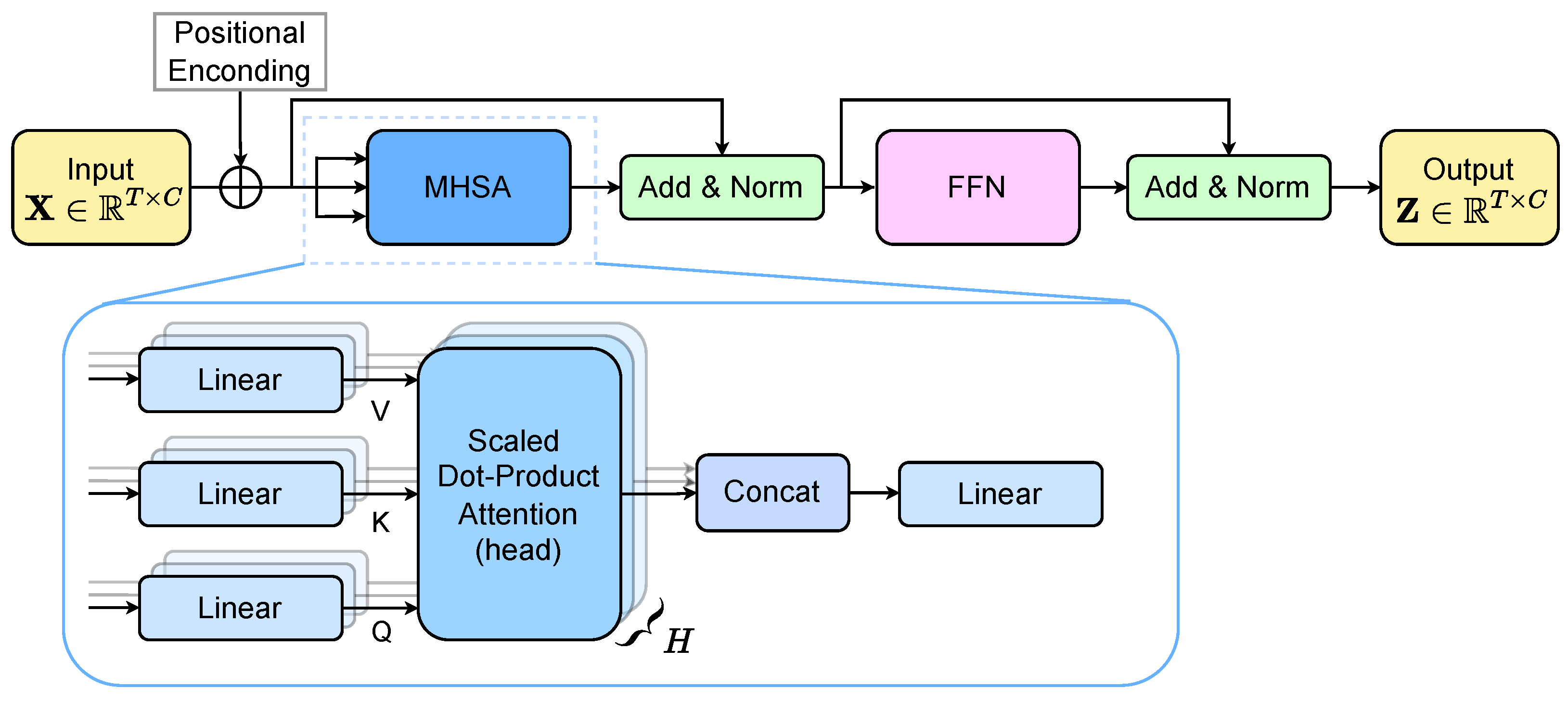
Figure 2.
Overview of the proposed T-GARNet model. Raw EEG segments are processed by a Transformer Encoder for temporal feature learning, followed by a Multi-Scale Gaussian connectivity module that generates multiple kernel-based connectivity matrices. These are refined via convolutional layers. The final objective combines binary cross-entropy with an -Rényi mutual information regularizer to enforce non-redundant connectivity features.
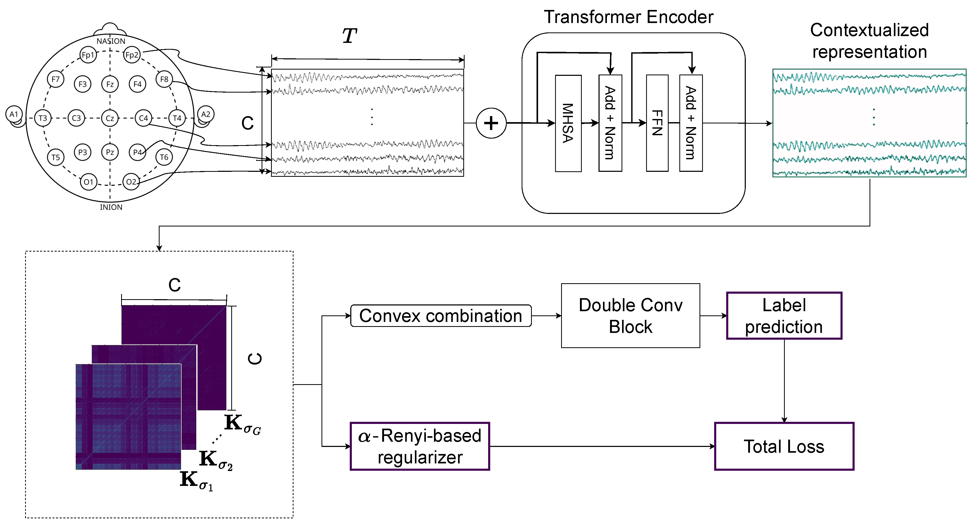
Figure 3.
Standard 10–20 system with 19 channels for EEG data acquisition (a). Example of the visual stimuli shown to children during EEG recording (b). EEG acquisition setup and cognitive task used during the experiment.
Figure 3.
Standard 10–20 system with 19 channels for EEG data acquisition (a). Example of the visual stimuli shown to children during EEG recording (b). EEG acquisition setup and cognitive task used during the experiment.
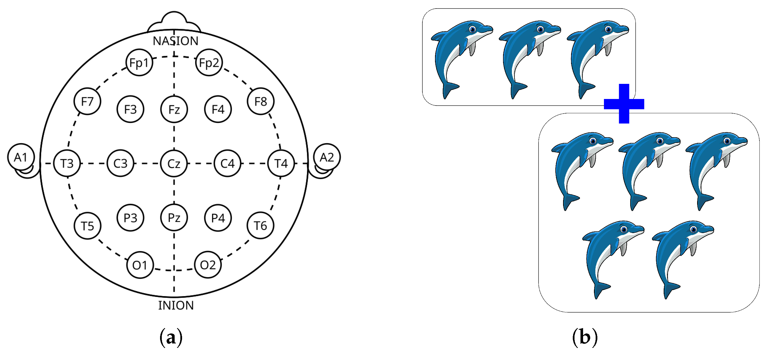
Figure 4.
Segmentation of raw EEG into 4-second windows (512 samples at 128 Hz) with 50% overlap. Sliding windows advance every 2 seconds, yielding consecutive partially overlapping epochs.
Figure 4.
Segmentation of raw EEG into 4-second windows (512 samples at 128 Hz) with 50% overlap. Sliding windows advance every 2 seconds, yielding consecutive partially overlapping epochs.
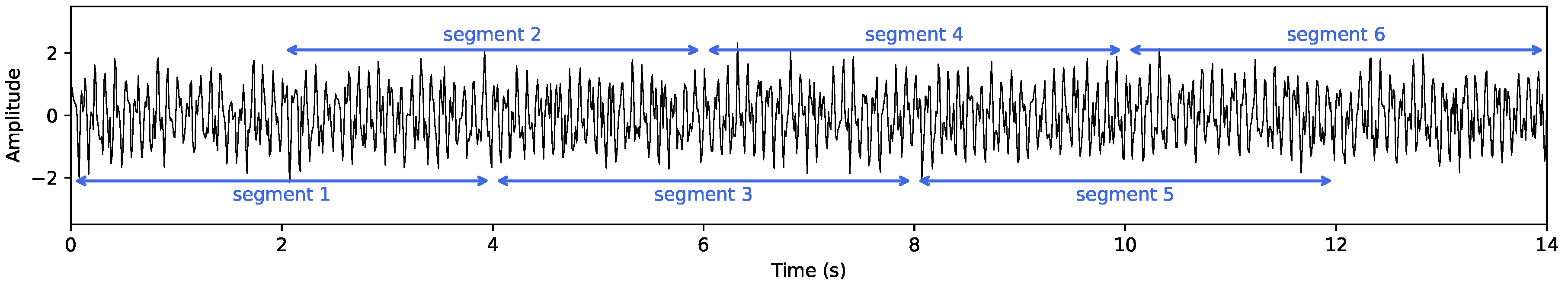
Figure 5.
Illustration of validation schemes using an example cohort of 10 subjects. Unlike naive segment-based splits, LOSO-CV and SGKF-CV strictly isolate subject identities across folds, ensuring reliable generalization estimates.
Figure 5.
Illustration of validation schemes using an example cohort of 10 subjects. Unlike naive segment-based splits, LOSO-CV and SGKF-CV strictly isolate subject identities across folds, ensuring reliable generalization estimates.
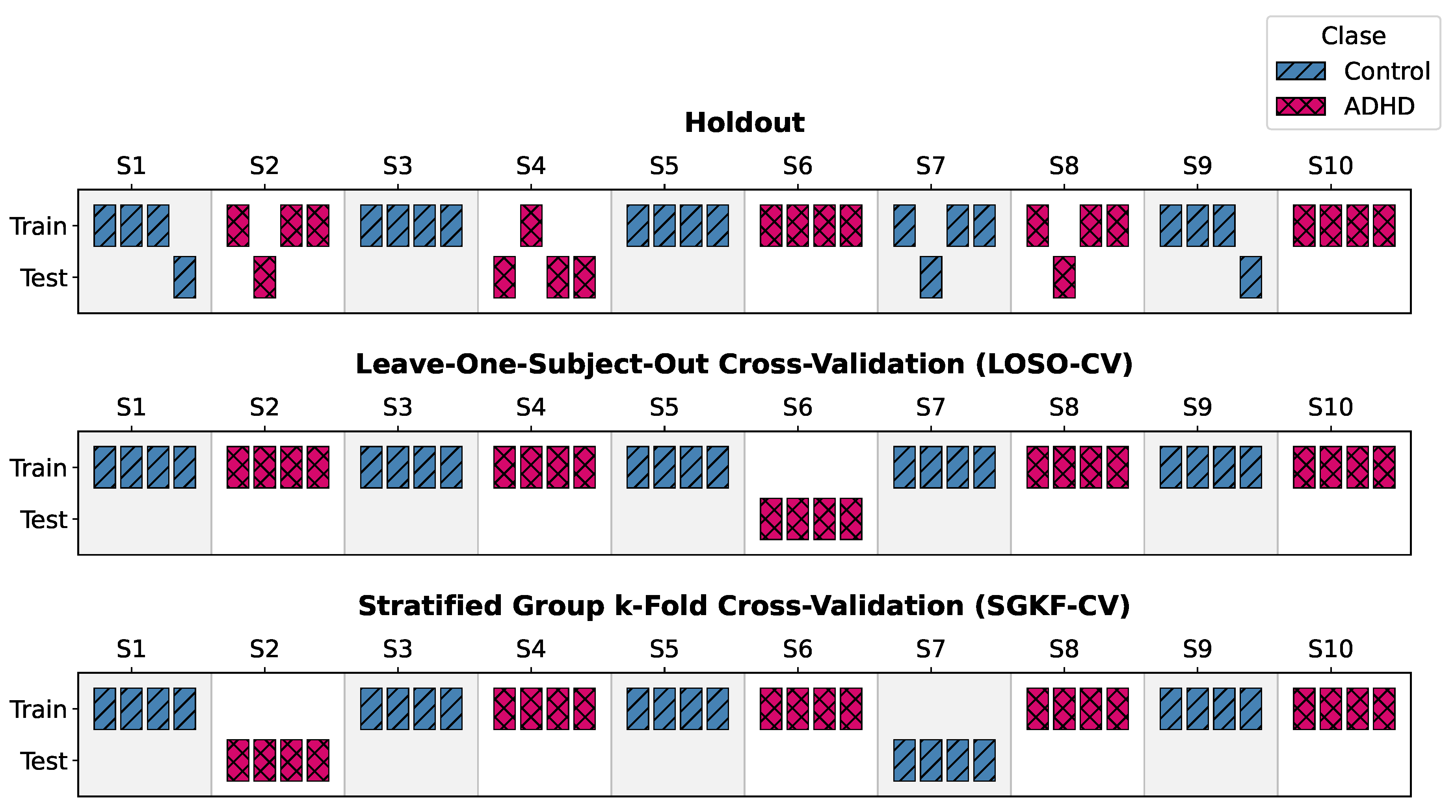
Figure 6.
Confusion matrices for the four strongest baselines under SGKF–CV: T-GARNet, ShallowConvNet, EEGNet, and CNN–LSTM. T-GARNet shows the most balanced classification profile, achieving high recall for ADHD cases while maintaining low false positive rates.
Figure 6.
Confusion matrices for the four strongest baselines under SGKF–CV: T-GARNet, ShallowConvNet, EEGNet, and CNN–LSTM. T-GARNet shows the most balanced classification profile, achieving high recall for ADHD cases while maintaining low false positive rates.
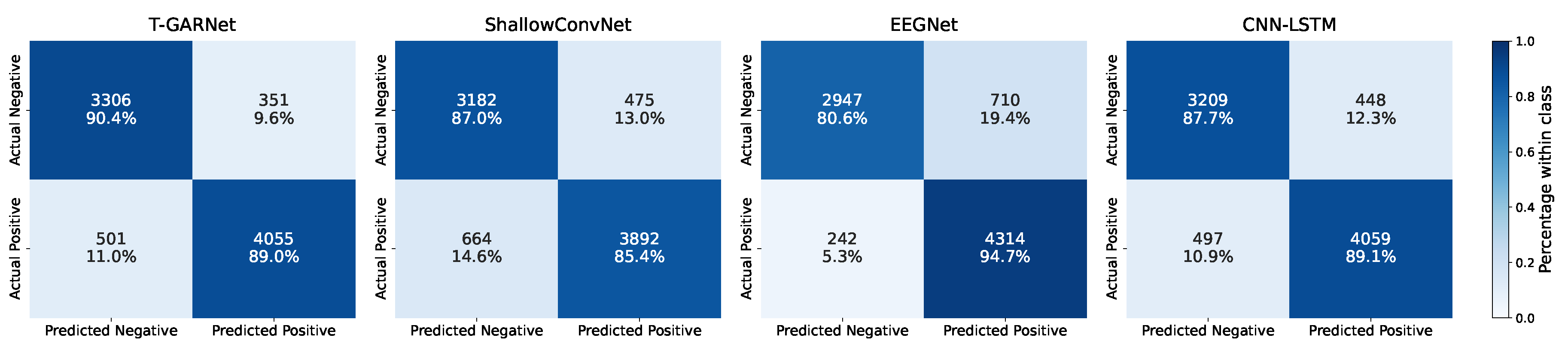
Figure 7.
Channel-wise importance distribution derived from the Transformer encoder weights across cross-validation folds.
Figure 7.
Channel-wise importance distribution derived from the Transformer encoder weights across cross-validation folds.
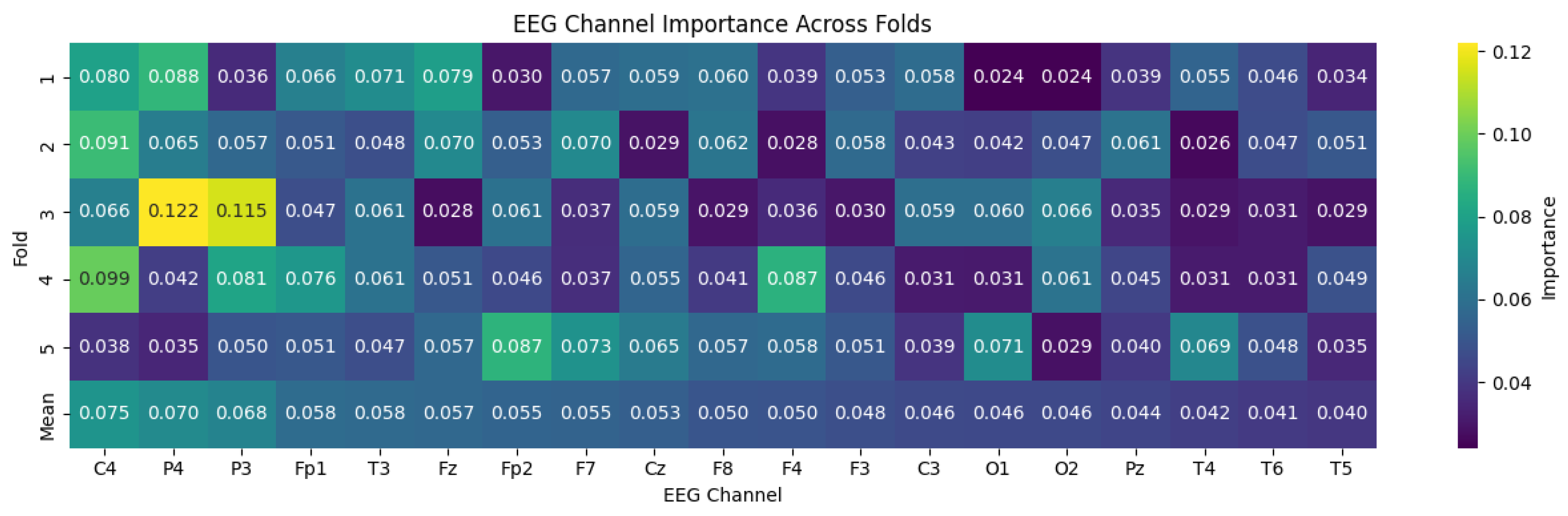
Figure 8.
Cumulative channel ablation analysis comparing ranked and random removal orders. Shaded area shows random mean ± standard deviation across 50 iterations.
Figure 8.
Cumulative channel ablation analysis comparing ranked and random removal orders. Shaded area shows random mean ± standard deviation across 50 iterations.

Figure 9.
Learned EEG connectivity patterns extracted from the Gaussian kernel layer of T-GARNet for a representative ADHD subject (left) and control subject (right). Each pattern reflects the segment-averaged connectivity matrix generated by the model in the fifth SGKF-CV fold, displayed using a connectivity threshold of 0.85 to highlight the strongest functional links.
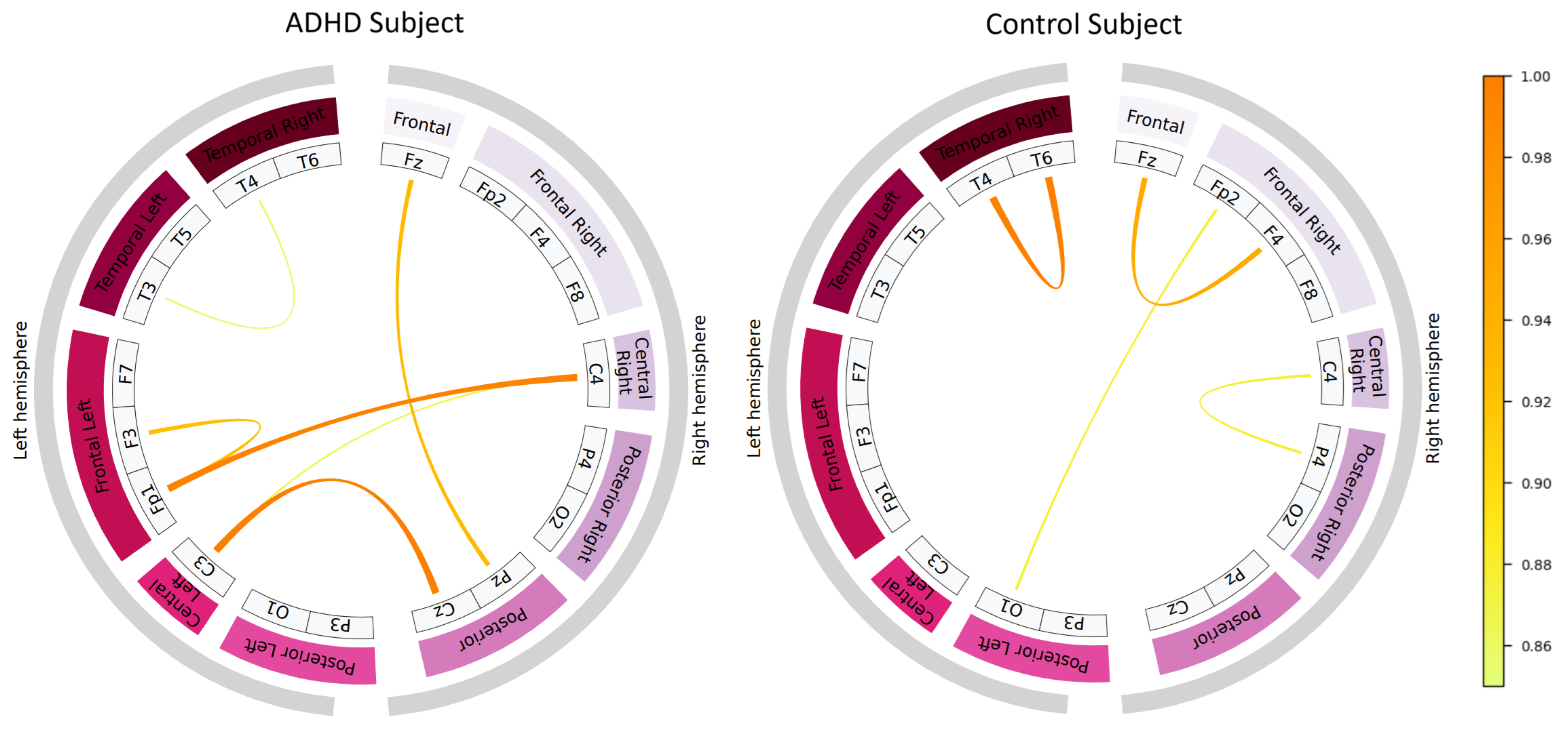
Figure 10.
Class–specific Grad-CAM++ relevance averaged over time and subjects from the test split of Fold 5. Left: ADHD class relevance. Middle: Control class relevance. Right: absolute difference map after joint min–max normalization. ADHD exhibits stronger frontocentral and right frontal–temporal importance, whereas Control shows greater relevance in lateral parietal and posterior regions.
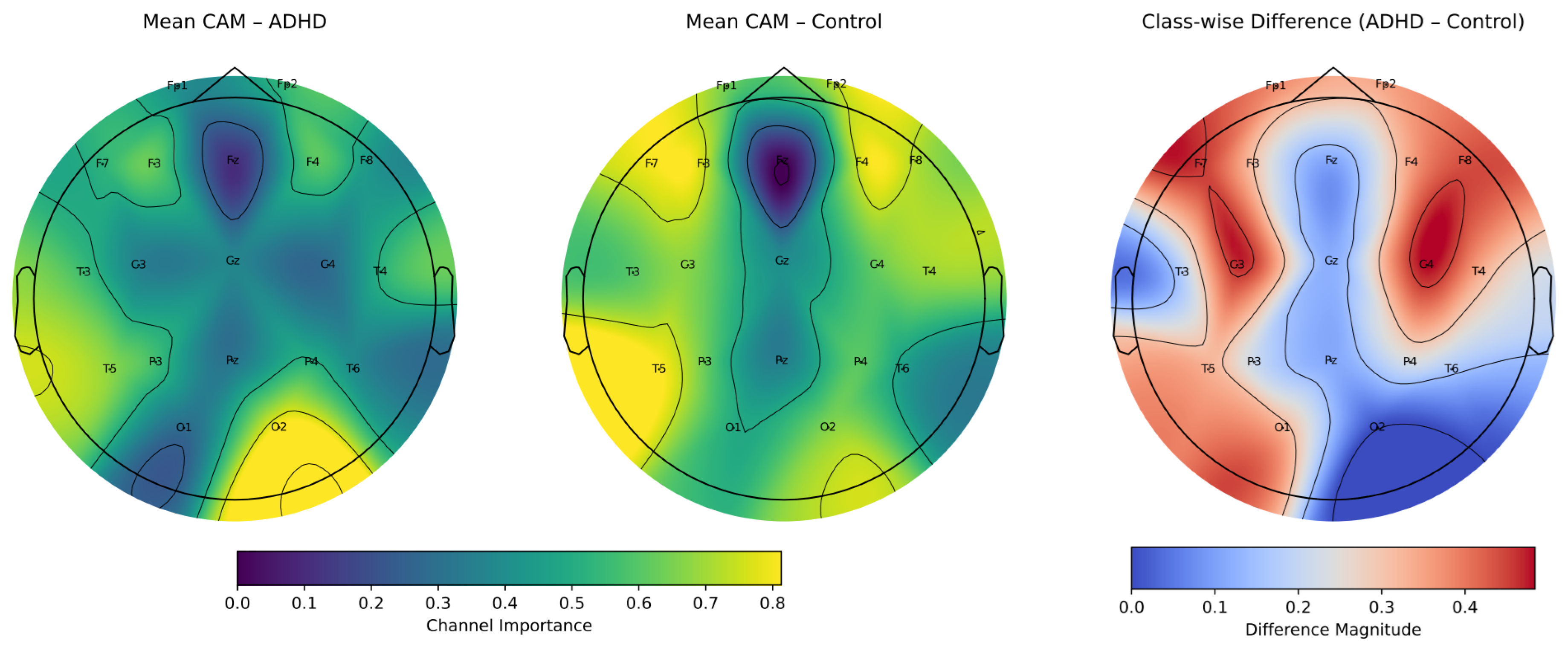

Table 1.
Summary of the EEG dataset used for ADHD classification.
| Source | IEEE DataPort [50] |
|---|---|
| Total Subjects | 121 children (61 ADHD, 60 control) |
| Age Range | 7–12 years |
| ADHD Group | 48 boys, 12 girls; mean age = 9.62 ± 1.75 years |
| Control Group | 50 boys, 10 girls; mean age = 9.85 ± 1.77 years |
| Diagnosis | DSM-IV, maximum 6 months of Ritalin use |
| EEG Channels | 19 (10–20 system): Fz, Cz, Pz, C3, T3, C4, T4, Fp1, Fp2, F3, F4, F7, F8, P3, P4, T5, T6, O1, O2 |
| Reference Electrodes | A1 and A2 (earlobes) |
| Sampling Rate | 128 Hz |
| Task Protocol | Cartoon-based visual attention task; 5–16 characters per image; continuous presentation based on response speed |
Table 2.
Architectural characteristics and design components of T-GARNet and baseline models for EEG-based ADHD classification
Table 2.
Architectural characteristics and design components of T-GARNet and baseline models for EEG-based ADHD classification
| Model | Trainable Params. | CNN | LSTM/RNN | Attention | Connectivity | Raw Data | Description |
|---|---|---|---|---|---|---|---|
| ShallowConvNet [32] | 33762 | yes | no | no | no | yes | Shallow convolutional architecture with squaring and log activations to approximate power features. |
| EEGNet [29] | 1666 | yes | no | no | no | yes | Compact architecture using depthwise and separable convolutions optimized for EEG decoding. |
| CNN-LSTM [33] | 8752 | yes | yes | no | no | yes | Convolutional feature extractor followed by recurrent layers for temporal modeling. |
| ANOVA-PCA SVM [19] | N/A | no | no | no | no | no | Handcrafted feature extraction and statistical dimensionality reduction with SVM classifier. |
| Multi-Stream Transformer [38] | 574082 | no | no | yes | no | no | Transformer encoders applied independently to spectral, spatial, and temporal inputs. |
| T-GARNet (this work) | 6942 | yes | no | yes | yes | yes | Transformer temporal modeling, Gaussian kernel connectivity, and Rényi entropy regularization. |
Table 3.
LOSO-CV accuracy performance across models.
| Model | ACC (%) |
|---|---|
| EEGNet | |
| CNN–LSTM | |
| ShallowConvNet | |
| Multi–Stream Transformer | |
| ANOVA–PCA SVM | |
| T-GARNet (This work) |
Table 4.
Performance comparison under the SGKF-CV protocol. T-GARNet shows robust performance; its main advantage is interpretability, discussed in the following sections.
Table 4.
Performance comparison under the SGKF-CV protocol. T-GARNet shows robust performance; its main advantage is interpretability, discussed in the following sections.
| Model | Accuracy (%) | Recall (%) | Precision (%) |
|---|---|---|---|
| ShallowConvNet | 84.67 ± 0.66 | 84.90 ± 0.53 | 86.15 ± 0.63 |
| EEGNet | 87.88 ± 1.26 | 87.12 ± 1.19 | 88.45 ± 1.53 |
| CNN-LSTM | 86.31 ± 2.12 | 86.01 ± 2.22 | 86.59 ± 2.07 |
| Multi-Stream Transformer | 74.05 ± 0.57 | 72.76 ± 0.69 | 74.68 ± 0.52 |
| ANOVA-PCA SVM | 66.47 ± 0.00 | 65.82 ± 0.00 | 66.59 ± 0.00 |
| T-GARNet (This work) | 88.32± 0.92 | 88.02± 0.97 | 88.65± 0.98 |
Table 5.
Statistical comparison of models under SGKF–CV. Lower rank is better. Significance refers to Wilcoxon post–hoc test with Holm correction against T-GARNet ().
Table 5.
Statistical comparison of models under SGKF–CV. Lower rank is better. Significance refers to Wilcoxon post–hoc test with Holm correction against T-GARNet ().
| Model | Avg. Rank | Wins (out of 50) | Significant vs T-GARNet |
|---|---|---|---|
| T-GARNet (proposed) | 2.28 | 19 | — |
| EEGNet | 2.36 | 9 | No |
| CNN-LSTM | 2.41 | 18 | No |
| ShallowConvNet | 3.12 | 4 | No |
| Multi-Stream Transformer | 5.24 | 0 | Yes |
| ANOVA-PCA SVM | 5.59 | 0 | Yes |
Disclaimer/Publisher’s Note: The statements, opinions and data contained in all publications are solely those of the individual author(s) and contributor(s) and not of MDPI and/or the editor(s). MDPI and/or the editor(s) disclaim responsibility for any injury to people or property resulting from any ideas, methods, instructions or products referred to in the content. |
© 2025 by the authors. Licensee MDPI, Basel, Switzerland. This article is an open access article distributed under the terms and conditions of the Creative Commons Attribution (CC BY) license (http://creativecommons.org/licenses/by/4.0/).
Copyright: This open access article is published under a Creative Commons CC BY 4.0 license, which permit the free download, distribution, and reuse, provided that the author and preprint are cited in any reuse.


