Submitted:
13 November 2025
Posted:
14 November 2025
You are already at the latest version
Abstract
Accurate streamflow forecasting is vital for sustainable water resource management but remains challenging due to pronounced spatiotemporal variability. This study evaluates two process-based models SWAT (comprehensive) and GWLF (parsimonious)—and a data-driven Random Forest (RF) model for monthly streamflow simulation in two contrasting Chinese basins: the humid southern basin (SSB) and the semi-arid northern basin (SRB). Using four statistical metrics (NSE, R2, MAE, RMSE), we assess model accuracy, robustness in capturing extremes, and sensitivity to hydrological characteristics and data availability. Results reveal consistently superior performance in the SSB across all models, with SWAT demonstrating the highest overall accuracy—especially for peak flows—due to its physically based structure. GWLF provides acceptable simulations with minimal data requirements, offering a practical alternative in data-limited regions like the SRB. RF performs well in the SSB under zero-lag conditions but requires hydrologically informed lag structures in the SRB. However, it consistently underestimates high flows due to its lack of physical constraints. The findings underscore that model selection must therefore be guided not only by predictive performance, but by the underlying hydrological context, data availability, and the need for physical realism in decision-making.
Keywords:
streamflow simulation
; hydrological modeling
; model comparison
; hydroclimatic variability
1. Introduction
Accurate streamflow forecasting is vital for effective water allocation, planning, and management [1,2]. However, streamflow exhibits high spatiotemporal variability due to uneven water distribution and the combined effects of precipitation, evapotranspiration, landscape characteristics, topography, climate change, and human activities [3,4,5,6]. This complexity introduces significant uncertainty in hydrological simulations across regions. Consequently, selecting modeling tools that align with local hydrological characteristics is critical to accurately represent streamflow dynamics [7,8,9,10].
Process-based hydrological models have long been used to simulate watershed-scale streamflow by explicitly representing key hydrological processes [11,12,13]. These models vary widely in structural complexity and data requirements. For instance, the Soil and Water Assessment Tool (SWAT) is among the most widely applied models in water resources management, demonstrating robust performance across diverse physical and climatic conditions [14,15]. However, its complex structure and extensive data demands often hinder its application in data-limited regions [16]. In contrast, the Generalized Watershed Loading Function (GWLF) model offers a more parsimonious alternative, requiring fewer inputs and offering greater operational flexibility [17,18], making it suitable for areas with constrained data availability [19,20]. Thus, the choice between these models involves a trade-off between process representation and practical feasibility.
In recent years, machine learning (ML) approaches have gained prominence in hydrology, driven by advances in big data and computational power [21,22,23]. Unlike process-based models, ML methods do not explicitly encode physical relationships; instead, they rely on mathematical functions to map inputs to outputs, thereby identifying complex, nonlinear patterns in data [24]. Models such as Random Forest (RF), Support Vector Machine (SVM), and Artificial Neural Networks (ANN) have been widely applied across hydrological tasks [23,25]. Among these, RF excels at handling high-dimensional datasets and automatically selecting relevant features, making it particularly effective for streamflow forecasting [26]. Nevertheless, ML models are frequently regarded as “black boxes” owing to poor interpretability, and their performance is strongly influenced by the underlying data and feature selection, warranting further evaluation of their applicability in regions with high data heterogeneity.
As the world’s largest developing country, China faces significant challenges related to water pollution and severe spatial imbalance in water resources—northern regions account for only 19% of the nation’s total water endowment despite hosting a large share of its population and economic activity [27,28]. Accurate hydrological prediction is therefore critical for understanding pollution dynamics and enabling equitable water allocation. While both process-based and ML models have achieved satisfactory performance in Chinese watersheds, few studies have systematically compared their applicability across regions with stark hydrological contrasts—particularly between water-rich southern and water-scarce northern basins.
This study selects two representative watersheds in northern and southern China to evaluate the performance of two process-based models of differing complexity—SWAT and GWLF—and a machine learning model (RF model) in monthly streamflow simulation. Model performance is assessed using four statistical metrics. The primary objective is to compare the applicability of these approaches across contrasting hydroclimatic regions. Specifically, the study includes: (1) calibration of SWAT and GWLF for streamflow simulation; (2) training of the RF model; (3) streamflow prediction using the calibrated/trained models; and (4) comparative analysis of model performance and regional suitability.
2. Materials and Methods
2.1. Study Area
This study was conducted in two contrasting watersheds: the Shahe River Basin (SRB) in northern China and the Shuai Shui Basin (SSB) in southern China. Although the two basins have similar elevation ranges and drainage areas, they exhibit a significant difference in water resources (Figure 1a). The SRB is located in the upstream area of the Yuqiao Reservoir in Tianjin (117°30′–118°0′E, 40°0′–42°20′N) and constitutes a key part of the Yuqiao Reservoir watershed, with a total drainage area of 905.2 km². Land use is dominated by forest land (44.06%) and agricultural land (37.78%). The basin’s topography is higher in the northeast and lower in the southwest, with a maximum elevation of 1100 m (Figure 1b,c). The long-term average annual precipitation and temperature are 650.7 mm and 12.9 °C, respectively, with rainfall concentrated during the summer months (July–September), marking a distinct wet season [17].
In contrast, the SSB is situated in southern Anhui Province (117°30′–118°10′E, 29°30′–29°50′N) and forms an important part of the upstream watershed of Qiandao Lake, covering a drainage area of 880.4 km². Land use is overwhelmingly dominated by forest land (90.4%), with only a small proportion of agricultural land (6.7%). The basin is characterized by mountainous and hilly terrain, with elevations ranging from 140 to 1614 m (Figure 1d,e). The long-term average annual precipitation is approximately 1700 mm, and the mean annual temperature is 15.6 °C. Precipitation is unevenly distributed throughout the year, with the majority occurring during spring and summer [29].
2.2. Data Source
Both SRB and SSB are equipped with a meteorological station and a hydrological station, as well as several rainfall stations (Figure 1b,d). The meteorological station data (including precipitation, maximum and minimum temperatures, average temperatures, relative humidity, wind speed and solar radiation) were obtained from the National Weather Science Data Center (http://data.cma.cn/). The rainfall stations data (including precipitation) and streamflow data from hydrological station were obtained from local hydrological bureau. The monthly Evapotranspiration data were available from Institute of Tibetan Plateau Research, Chinese Academy of Sciences, and all these data were used to construct hydrological model (including SWAT and GWLF model) and RF model. In addition, spatial data including digital elevation model (DEM), land use, soils are also required in the hydrological model. The DEM is derived from the Geospatial Data Cloud (https://www.gscloud.cn/) with a resolution of 30×30 m, and the land use and soil is derived from the Resource and Environmental Science and Data Center (https://www.resdc.cn/), with a scale of 1:1000000.

Table 1.
Types, source, resolution and description of the model datasets.
| Data Type | Data source | Resolution | Description |
| Meteorological data | National Weather Science Data Center (http://data.cma.cn/) |
daily | Precipitation, Temperatures, Relative humidity, Wind speed, Solar radiation |
| Rainfall station data | Local hydrological bureau | daily | Precipitation |
| Evapotranspiration data | Institute of Tibetan Plateau Research, Chinese Academy of Sciences (http://data.tpdc.ac.cn/zh-hans/) |
monthly | Evapotranspiration |
| Hydrological data | Local hydrological bureau | daily | Streamflow |
| DEM | Geospatial Data Cloud (https://www.gscloud.cn/) |
30m | Digital elevation model |
| Land use | Resource and Environmental Science and Data Center (https://www.resdc.cn/) | 1:1000000 | Land use type |
| Soil | Resource and Environmental Science and Data Center (https://www.resdc.cn/) | 1:1000000 | Soil type |
2.3. Model Description
2.3.1. SWAT Model Description
The SWAT model is a process-based, semi-distributed hydrological model developed by the USDA Agricultural Research Center, characterized by robust physical mechanisms. This model divides the watershed into Hydrological Response Units (HRUs) based on land use types, soil types, and slopes within the study area. It conducts water quantity and quality simulations based on the hydrological response units and their water balances. The SWAT model employs the curve number method for runoff calculation and utilizes the Muskingum method for channel routing. Independently, SWAT calculates water yield for each Hydrological Response Unit (HRU) and then consolidates these values at the sub-basin level. Since its development, the SWAT model has been widely applied in streamflow and water quality simulations, making it one of the most extensively used hydrological models [30,31].
2.3.2. GWLF Model Description
The GWLF model, developed by Cornell University and Pennsylvania State University, is a combined distributed/lumped parameter, continuous watershed model [32]. Over the past decades, the GWLF model has been secondarily developed in different platforms. Here, we use the modified GWLF model (ReNuMa model) for streamflow simulation. The model is not spatially conceptualized and each area is considered uniformly in terms of soil and cover [19]. Soil moisture contains unsaturated zone, shallow saturated zone and deep saturated zone parameters. The model using a daily time step and the curve number method to simulate daily hydrologic water balance [33,34]. Compared with the SWAT model, this model has more moderate data requirements and a more flexible mode of operation, and has been widely used around the world.
2.3.3. RF Model Description
RF model is an integrated learning model, which is a classifier method combining bagging integrated learning theory with random subspaces, and has been widely used to deal with classification and regression issues [7,35]. The RF model mainly consists of two parts: the training sample subset and the subclassification model, each tree of the RF model is drawn from a random subset of the original sample set. Based on the extracted M sets of training samples, M sub-prediction models can be constructed, and based on each sub-prediction model, a corresponding forecast result can be obtained (Figure 2). The final forecast value is determined by voting (for categorical variables) or averaging (for continuous numerical variables) among the M sub-prediction models. Streamflow simulation mainly involves the application of RF model in regression.
2.4. Model Settings and Evaluating
2.4.1. SWAT Model
By setting the stream definition thresholds in the SWAT model, the SSB and SRB were divided into 15 and 19 sub-basins respectively, with 89 and 116 HURs (Figure 1). The Penman–Monteith equation and the SCS curve number method was applied in the model to calculate potential evapotranspiration and rainfall-runoff. The SWAT-CUP with SUFI-2 algorithm was adopted to calibrate the hydrological parameters in the SWAT model and fifteen parameters were selected for five hundred simulations iteration for twice. The periods 2007-2013 and 2001-2007 were assigned for calibration in SSB and SRB, both with a one-year for warming-up, and 2014-2016 and 2008-2010 were used for validate for streamflow, respectively. The chosen parameters were calibrated using monthly time steps, and the accuracy of the streamflow simulation results is judged by the Nash-efficiency coefficient (NSE) and R2 value.
2.4.2. GWLF Model
Streamflow simulation in the GWLF model typically requires meteorological data (including watershed-averaged precipitation and temperature), observed streamflow records, and spatially distributed land use information. In this study, the Thiessen polygon method in ArcGIS was used to compute the basin-wide average precipitation and temperature from multiple rainfall and meteorological stations. The modified GWLF model, known as the ReNuMa model, was applied, and its built-in calibration function was used to calibrate streamflow. The model uses a programming solver method to keep the simulated values as close as possible to the predicted values. As well, the time settings for the warm-up, calibration and validation periods in the SSB and SRB are consistent with in the SWAT model, and the reliable of the model is based on the values of NSE and R2.
2.4.3. RF Model
The RF model was performed using the “RandomForest” package in R, six variables were selected as independent variable inputs to the model, including precipitation (P), evapotranspiration (ET), average temperatures (AT), relative humidity (RH), wind speed (WS) and solar radiation (SR) and all these variables are processed into the form of a monthly scale. Considering the rainfall’s lag has a significant influence on the prediction of streamflow, the cross-correlation analysis was used to determine the number of lag days of rainfall. Here, several scenarios were constructed and tested in order to estimate monthly streamflow (Table 2). The scenarios consider the effect of different rainfall’s lag days on streamflow simulation, with 1st, 2nd and 3rd day’s lagged rainfall along with the streamflow.
2.4.4. Performance Evaluation Indicators
Four statistical indicators were chosen to evaluate the fits of the models during the calibration and the validator period, including the Coefficient of determination (R2), Nash-efficiency coefficient (NSE), Mean absolute error (MAE) and Root Mean Square Error (RMSE).
The corresponding formulas are provided in Table 3, where Ot denotes the observed streamflow value, and Oavg represents the average observed value of the streamflow, Pt indicates the predicted value, and Pavg represents the average predicted value of the streamflow. The R2 measures the linear relationship between the simulated and observed data, and NSE is used to characterize the variance between observed and simulated data, the closer R2 and NSE values are to 1, the better the model performance is. In contrast, MAE and RMSE measure the average magnitude of prediction errors, reflecting the overall deviation between predicted and observed values. Both metrics range from 0 to ∞.
3. Results and Discussion
3.1. SWAT and GWLF Calibration
Fifteen and four frequently used streamflow calibration parameters were selected for model calibration in the SWAT and GWLF models, respectively. The parameter descriptions, default value ranges and final calibration values are listed in Table 4.
The calibrated parameter values exhibit significant spatial variability across the mechanistic models applied for streamflow simulation in the southern and northern basins of China. In the SWAT model, the CN2 value of SSB was higher than that of SRB, indicating a greater potential for surface runoff generation in the south. Conversely, the SRB exhibits a high SOL_AWC value of 0.88, reflecting typical characteristics of watersheds in northern China, where arid conditions lead to a higher soil available water capacity [36]. ALPHA_BF governs the rate at which groundwater contributes to streamflow; a larger ALPHA_BF value indicates more stable baseflow. Since the SSB is located in a humid southern region with consistently high rainfall and sustained high soil moisture, its groundwater discharge is more stable compared to the drier northern SRB. LAT_TTIME and SURLAG values reflect the retention effect of streamflow to some extent, with longer retention times for SRB and shorter retention times for SSB [37].
In the GWLF model, the CN2 values and SOL_AWC for the SSB and SRB exhibit patterns consistent with those observed in the SWAT model. These similarities are primarily attributed to watershed-specific soil properties: the SSB is predominantly underlain by red soils, while the SRB is dominated by brown soils. Compared to red soils, brown soils typically have lower permeability but greater water-holding capacity [38]. The recession coefficient and seepage coefficient are the most critical parameters governing groundwater processes [39]. The higher values of these parameters in the SSB indicate more active and intense groundwater dynamics. Overall, the variability in model parameters across catchments reflects fundamental differences in their underlying hydrological processes.
3.2. RF Training and Testing
In the RF model, input variables significantly influence forecasting outcomes. In this study, we selected six readily available, continuous variables that are closely related to streamflow to construct the RF model, and we considered different scenarios based on varying runoff retention periods (i.e., lag days). The dataset was split into training and testing subsets, with 75% allocated for training and 25% for testing. A larger training sample was used to ensure the model captures the majority of the underlying data patterns and variability. Model performance was evaluated across all scenarios, with the RF hyperparameters fixed at 200 trees and maximum depth allowed for tree expansion. Results show that the RF model achieves low computational time across all scenarios, demonstrating its efficiency for streamflow forecasting under different retention-day configurations.
3.3. Analysis and Comparison of the Model Performance in SRB and SSB
The model calibration and validation performance metrics in SRB and SSB are presented in Table 5. It is evident that the values of the four statistical metrics differ slightly between the calibration and validation periods in both watersheds. Overall, the models perform significantly better in the SSB than in the SRB. In the SSB, all three models achieve R2 and NSE values exceeding 0.85 during both calibration and validation, along with low MAE and RMSE values, indicating reliable and accurate monthly streamflow predictions.
Among the three models, SWAT demonstrates the best performance in the SSB, yielding the highest R² and NSE values and the lowest MAE and RMSE across both calibration and validation periods. For the RF model, Scenario I (i.e., zero lag or shortest retention period) yields the best validation performance, suggesting that the rainfall–streamflow response in the SSB exhibits a weak retention effect, with streamflow reacting rapidly to precipitation inputs.
In contrast, model performance in the SRB shows greater variability. SWAT outperforms GWLF consistently in both calibration and validation phases, while the RF model performs well during training but only moderately during testing—reflecting the more complex, nonlinear rainfall–runoff dynamics characteristic of semi-arid regions. For the RF model in the SRB, Scenario III (i.e., incorporating a multi-day runoff lag) achieves the best predictive performance, which can be attributed to the presence of a discernible time lag between rainfall and runoff response in the watershed.
Figure 3 and Figure 4 present the monthly streamflow simulations for the SRB and SSB, respectively, using the SWAT, the GWLF, and the RF model under their optimal scenarios. Both process-based models and the data-driven RF model effectively capture the temporal dynamics of streamflow, demonstrating their general applicability. However, visual inspection of hydrographs and scatter plots reveals markedly better agreement between observed and simulated streamflow in the SSB than in the SRB. This discrepancy is consistent with the climatic contrasts between the two basins: monthly precipitation ranges from 0–500 mm in the SRB versus 0–1000 mm in the SSB, while corresponding streamflow ranges from 0–30 m3/s to 0–250 m3/s, respectively. These differences underscore the strong influence of regional climate on model performance.
Furthermore, in the SRB, observed monthly streamflow hydrographs do not align closely with precipitation timing in the SWAT and GWLF simulations, whereas in the SSB, a tighter correspondence is evident. This observation aligns with model parameterization results, indicating a more pronounced rainfall–runoff retention effect in the semi-arid northern watershed. The disparity arises from fundamental differences in runoff generation mechanisms: the SRB, situated in an arid to semi-arid climate zone, experiences predominantly short-duration, high-intensity storms that generate infiltration-excess runoff [40]. In contrast, the SSB, located in a humid to semi-humid region with more sustained rainfall, is dominated by saturation-excess runoff [41]. This hydroclimatic contrast is also reflected in the optimal configurations of the RF model: Scenario I, which assumes minimal lag between rainfall and runoff, performs best in the SSB, while Scenario III, incorporating a multi-day lag, yields superior results in the SRB—highlighting the differing temporal dynamics of the rainfall–runoff response in the two basins.
Additionally, the process-based models (SWAT and GWLF) demonstrate a greater capacity to capture peak flow events, whereas the RF model exhibits markedly reduced accuracy under high-flow extremes (Figure 3 and 4)—a pattern consistent with findings from other studies on data-driven hydrological modeling [42]. This discrepancy arises because SWAT and GWLF are grounded in explicit physical equations that represent key hydrological processes such as overland flow, interflow, and baseflow, enabling them to physically extrapolate beyond observed conditions and respond plausibly to extreme rainfall events. In contrast, the RF model is a data-driven, black-box approach that effectively learns nonlinear input-output relationships, including those between precipitation, temperature, and streamflow, but is fundamentally constrained by the scope and representativeness of its training data. When extreme high-flow events are scarce or absent in the training set, RF lacks a physical mechanism to generalize to unprecedented conditions, often resulting in systematic underestimation of peak flows [42]. Such underestimation is further exacerbated by the inherent rarity of extreme events in historical records, which leads to insufficient sampling of high-intensity rainfall scenarios [43]. Consequently, when input variables such as rainfall intensity fall outside the range of observed training data, data-driven models tend to produce smoothed or averaged responses, further compromising their ability to capture the true magnitude of peak flows.
3.4. Model Insights and Implications for Future Water Management
Driven by the combined effects of climate change and intensifying anthropogenic activities, natural runoff processes have become highly nonlinear and increasingly complex, posing significant challenges for traditional hydrological models to fully capture their dynamics [44,45,46,47,48]. Machine learning methods offer a promising new pathway for hydrological forecasting. However, their performance is critically dependent on the scientific selection of input variables and the rational optimization of model architecture—precise feature engineering and structural design are essential prerequisites for achieving reliable predictions [43].
In this context, a comparative assessment of process-based models (SWAT and GWLF) and data-driven approaches (RF model) across northern and southern Chinese watersheds yields critical insights for future water resource management. Process-based models consistently outperformed the RF model in simulating peak flow events under extreme hydrological conditions, particularly in southern basins where intensified rainfall extremes linked to climate change are more prevalent. This advantage stems from their mechanistic representation of key hydrological processes—including overland flow, interflow, and baseflow—which enables physically plausible extrapolation beyond the range of observed data [49].
In contrast, the RF model systematically underestimated peak flows in both regions, especially when confronted with non-stationary conditions arising from rapid urbanization, reservoir regulation, and groundwater depletion in the north, or unprecedented rainfall intensities in the south—scenarios that are typically underrepresented or absent in historical training datasets [42]. While the RF model demonstrated reasonable accuracy for moderate flows in data-rich and relatively stable environments, its predictive reliability deteriorated sharply under anthropogenic non-stationarity and climate regime shifts, underscoring its inherent vulnerability to extrapolation beyond the limits of training data.
These findings affirm that process-based models remain indispensable for long-term planning under evolving climate and land-use scenarios, particularly in regions characterized by complex human–water interactions. Meanwhile, data-driven approaches can become robust tools only when augmented with explicit physical constraints or integrated into hybrid modeling frameworks [50].
From a management perspective, these results suggest that water resource strategies must be regionally differentiated [51]. In northern watersheds, where human interventions dominate hydrological trends, SWAT and GWLF should be prioritized to evaluate the long-term impacts of policies such as groundwater recharge programs, irrigation efficiency upgrades, and reservoir operation rules. In southern watersheds, where flood risk is escalating due to climate-driven extreme rainfall, process-based models are essential for designing resilient infrastructure, updating flood hazard maps, and informing early warning systems under future climate scenarios. The RF model, despite its limitations in extreme event prediction, holds value in operational settings for short-term flow forecasting and real-time monitoring, particularly when calibrated with high-frequency observational data and constrained by physical bounds—for example, the maximum possible runoff under given antecedent conditions [52].
We therefore advocate for an integrated modeling strategy: deploying process-based models as the backbone for scenario analysis and policy evaluation, while integrating machine learning for adaptive, data-driven refinement of forecasts and residual error correction [53]. This hybrid paradigm not only enhances predictive accuracy but also ensures scientific credibility, enabling water managers to make informed, resilient, and adaptive decisions in an era of accelerating environmental uncertainty.
5. Conclusions
This study systematically evaluates the regional applicability of two process-based models (SWAT and GWLF) and a data-driven machine learning model (RF) for monthly streamflow simulation across two hydroclimatically contrasting basins in China: the humid southern basin(SSB) and the semi-arid northern basin(SRB). The results indicate that all models perform markedly better in the SSB, achieving high Nash–Sutcliffe efficiency (NSE) and coefficient of determination (R2) values (>0.85), along with low mean absolute error (MAE) and root mean square error (RMSE). SWAT yields the highest overall accuracy in both basins, particularly in simulating peak flows, which can be attributed to its comprehensive physics-based representation of hydrological processes. GWLF, despite its lower complexity and reduced input requirements, produces reasonably accurate simulations, making it particularly useful in data-limited contexts such as the SRB, though it exhibits limitations in capturing extreme flow events. RF performs well in the SSB under zero-lag conditions, reflecting a rapid rainfall–runoff response, but necessitates the incorporation of multi-day lags in the SRB to account for delayed infiltration-excess runoff. However, RF consistently underestimates high-flow events, especially in the SRB, owing to its reliance on training data and absence of embedded physical mechanisms. The pronounced performance disparity between the two basins underscores the critical influence of regional hydrological characteristics—such as precipitation regimes, soil properties, and dominant runoff generation mechanisms (saturation-excess versus infiltration-excess)—on model suitability. We conclude that SWAT is the more reliable choice for physically consistent, extreme-event forecasting in heterogeneous environments; GWLF provides a practical, low-data-footprint alternative for regional-scale applications; and RF serves as an efficient, high-accuracy tool in data-rich, climatically stable basins—provided lag structures are hydrologically justified. Model selection must therefore be guided not only by predictive performance, but by the underlying hydrological context, data availability, and the need for physical realism in decision-making.
Author Contributions
H.C.: Conceptualization, Data curation, formal analysis, and original draft. R.Y.: Methodology, supervision, and writing (reviewing and editing). F.Z.: Methodology, supervision, software, and writing (review and editing). J.R.: Methodology, supervision, software, and writing (review and editing). T.W.: Supervision and writing (reviewing and editing). All authors have read and agreed to the published version of the manuscript.
Funding
This research was funded by the Natural Science Foundation of Anhui Province of China (Grant No. 2208085US06) and the Jiangxi Province High-level and High-skilled Leading Talents Cultivation Project (2025).
Data Availability Statement
The data that support the findings of this study are available on request from the corresponding author (H.C.).
Acknowledgments
The constructive comments and suggestions by the journal referees are gratefully acknowledged.
Conflicts of Interest
The authors declare no conflicts of interest.
References
- Xl, A.; Xy, B.; Shuang, Z. A.; Zx, A.; Lm, C.; & Jing, P. A. J. J. o. H. A hybrid support vector regression framework for streamflow forecast. Journal of Hydrology. 2019, 568, 184–193.
- Reis, G. B.; da Silva, D. D.; Fernandes Filho, E. I.; Moreira, M. C.; Veloso, G. V.; Fraga, M. d. S.; & Pinheiro, S. A. R. Effect of environmental covariable selection in the hydrological modeling using machine learning models to predict daily streamflow. Journal of Environmental Management. 2021, 290, 112625.
- Sarah, S.; Shah, W.; & Ahmed, S. Modeling and comparing streamflow simulations in two different montane watersheds of western himalayas. Groundwater for Sustainable Development. 2021, 15, 100689.
- Shi, R.; Wang, T.; Yang, D.; & Yang, Y. Streamflow decline threatens water security in the upper Yangtze river. Journal of Hydrology. 2022, 606, 127448. [Google Scholar] [CrossRef]
- Wu, L.; Zhang, X.; Hao, F.; Wu, Y.; Li, C.; & Xu, Y. Evaluating the contributions of climate change and human activities to runoff in typical semi-arid area, China. Journal of Hydrology. 2020, 590, 125555. [Google Scholar] [CrossRef]
- Feng, Z.-k.; Liu, S.; Niu, W.-j.; Li, B.-j.; Wang, W.-c.; Luo, B.; & Miao, S.-m. A modified sine cosine algorithm for accurate global optimization of numerical functions and multiple hydropower reservoirs operation. Knowledge-Based Systems. 2020, 208, 106461. [Google Scholar] [CrossRef]
- Abbasi, M.; Farokhnia, A.; Bahreinimotlagh, M.; & Roozbahani, R. A hybrid of Random Forest and Deep Auto-Encoder with support vector regression methods for accuracy improvement and uncertainty reduction of long-term streamflow prediction. Journal of Hydrology. 2021, 597, 125717. [Google Scholar] [CrossRef]
- Liu, Y.; Ji, C.; Wang, Y.; Zhang, Y.; Hou, X.; & Ma, H. Consideration of streamflow forecast uncertainty in the development of short-term hydropower station optimal operation schemes: A novel approach based on mean-variance theory. Journal of Cleaner Production. 2021, 304, 126929. [Google Scholar] [CrossRef]
- Lorenzo-Lacruz, J.; Morán-Tejeda, E.; Vicente-Serrano, S. M.; Hannaford, J.; García, C.; Peña-Angulo, D.; & Murphy, C. Streamflow frequency changes across western Europe and interactions with North Atlantic atmospheric circulation patterns. Global and Planetary Change. 2022, 212, 103797. [Google Scholar] [CrossRef]
- Teutschbein, C.; Grabs, T.; Karlsen, R. H.; Laudon, H.; & Bishop, K. Hydrological response to changing climate conditions: Spatial streamflow variability in the boreal region. Water Resources Research. 2015, 51, 9425–9446. [Google Scholar] [CrossRef]
- Sadler, J. M.; Appling, A. P.; Read, J. S.; Oliver, S. K.; Jia, X.; Zwart, J. A.; & Kumar, V. Multi--Task Deep Learning of Daily Streamflow and Water Temperature. Water Resources Research. 2022, 58, e2021WR030138. [Google Scholar] [CrossRef]
- Yuan, Y.; & Koropeckyj-Cox, L. SWAT model application for evaluating agricultural conservation practice effectiveness in reducing phosphorous loss from the Western Lake Erie Basin. Journal of Environmental Management. 2022, 302, 114000. [Google Scholar] [CrossRef]
- Cho, K. H.; Pachepsky, Y. A.; Oliver, D. M.; Muirhead, R. W.; Park, Y.; Quilliam, R. S.; & Shelton, D. R. Modeling fate and transport of fecally-derived microorganisms at the watershed scale: State of the science and future opportunities. Water Research. 2016, 100, 38–56. [Google Scholar] [CrossRef]
- Chen, L.; Wei, G.; Zhong, Y.; Wang, G.; & Shen, Z. Targeting priority management areas for multiple pollutants from non-point sources. Journal of Hazardous Materials. 2014, 280, 244–251. [Google Scholar] [CrossRef]
- Shen, Z.; Zhong, Y.; Huang, Q.; & Chen, L. Identifying non-point source priority management areas in watersheds with multiple functional zones. Water Research. 2015, 68, 563–571. [Google Scholar] [CrossRef] [PubMed]
- Tan, M. L.; Gassman, P. W.; Yang, X.; & Haywood, J. A review of SWAT applications, performance and future needs for simulation of hydro-climatic extremes. Advances in Water Resources. 2020, 143, 103662. [Google Scholar] [CrossRef]
- Sha, J.; Liu, M.; Wang, D.; Swaney, D. P.; & Wang, Y. Application of the ReNuMa model in the Sha He river watershed: Tools for watershed environmental management. Journal of Environmental Management. 2013, 124, 40–50. [Google Scholar] [CrossRef]
- Rumph Frederiksen, R.; & Molina-Navarro, E. The importance of subsurface drainage on model performance and water balance in an agricultural catchment using SWAT and SWAT-MODFLOW. Agricultural Water Management. 2021, 255, 107058. [Google Scholar] [CrossRef]
- Niraula, R.; Kalin, L.; Srivastava, P.; & Anderson, C. J. Identifying critical source areas of nonpoint source pollution with SWAT and GWLF. Ecological Modelling. 2013, 268, 123–133. [Google Scholar] [CrossRef]
- Santos, F. M. d.; de Oliveira, R. P.; & Mauad, F. F. Evaluating a parsimonious watershed model versus SWAT to estimate streamflow, soil loss and river contamination in two case studies in Tietê river basin, São Paulo, Brazil. Journal of Hydrology: Regional Studies. 2020, 29, 100685. [Google Scholar] [CrossRef]
- Chu, H.; Wei, J.; Wu, W.; Jiang, Y.; Chu, Q.; & Meng, X. A classification-based deep belief networks model framework for daily streamflow forecasting. Journal of Hydrology. 2021, 595, 125967. [Google Scholar] [CrossRef]
- Kumar, A.; Ramsankaran, R.; Brocca, L.; & Muñoz-Arriola, F. A simple machine learning approach to model real-time streamflow using satellite inputs: Demonstration in a data scarce catchment. Journal of Hydrology. 2021, 595, 126046. [Google Scholar] [CrossRef]
- Niu, W.-j.; & Feng, Z.-k. Evaluating the performances of several artificial intelligence methods in forecasting daily streamflow time series for sustainable water resources management. Sustainable Cities and Society. 2021, 64, 102562. [Google Scholar] [CrossRef]
- Jimeno-Sáez, P.; Martínez-España, R.; Casalí, J.; Pérez-Sánchez, J.; & Senent-Aparicio, J. A comparison of performance of SWAT and machine learning models for predicting sediment load in a forested Basin, Northern Spain. CATENA. 2022, 212, 105953. [Google Scholar] [CrossRef]
- Ferreira, R. G.; Silva, D. D. d.; Elesbon, A. A. A.; Fernandes-Filho, E. I.; Veloso, G. V.; Fraga, M. d. S.; & Ferreira, L. B. Machine learning models for streamflow regionalization in a tropical watershed. Journal of Environmental Management. 2021, 280, 111713. [Google Scholar] [CrossRef]
- Yaseen, Z. M.; El-shafie, A.; Jaafar, O.; Afan, H. A.; & Sayl, K. N. Artificial intelligence based models for stream-flow forecasting: 2000–2015. Journal of Hydrology. 2015, 530, 829–844. [Google Scholar] [CrossRef]
- Jiang, J.; Li, S.; Hu, J.; & Huang, J. A modeling approach to evaluating the impacts of policy-induced land management practices on non-point source pollution: A case study of the Liuxi River watershed, China. Agricultural Water Management. 2014, 131, 1–16. [Google Scholar] [CrossRef]
- Yuan, F.; Wei, Y. D.; Gao, J.; & Chen, W. Water crisis, environmental regulations and location dynamics of pollution-intensive industries in China: A study of the Taihu Lake watershed. Journal of Cleaner Production. 2019, 216, 311–322. [Google Scholar] [CrossRef]
- Chen, H.; Wang, C.; Ren, Q.; Liu, X.; Ren, J.; Kang, G.; & Wang, Y. Long-term water quality dynamics and trend assessment reveal the effectiveness of ecological compensation: Insights from China’s first cross-provincial compensation watershed. Ecological Indicators. 2024, 169, 112853. [Google Scholar] [CrossRef]
- Li, M.; Di, Z.; & Duan, Q. Effect of sensitivity analysis on parameter optimization: Case study based on streamflow simulations using the SWAT model in China. Journal of Hydrology. 2021, 603, 126896. [Google Scholar] [CrossRef]
- Jeyrani, F.; Morid, S.; & Srinivasan, R. Assessing basin blue–green available water components under different management and climate scenarios using SWAT. Agricultural Water Management. 2021, 256, 107074. [Google Scholar] [CrossRef]
- Evans, B. M.; Lehning, D. W.; Corradini, K. J.; Petersen, G. W.; & Robillard, P. D. J. j. s. h. A Comprehensive GIS-Based Modeling Approach for Predicting Nutrient Loads in Watersheds. Journal of Spatial Hydrology. 2002, 2, 1–18. [Google Scholar]
- Sharifi, A.; Yen, H.; Boomer, K. M. B.; Kalin, L.; Li, X.; & Weller, D. E. Using multiple watershed models to assess the water quality impacts of alternate land development scenarios for a small community. CATENA. 2017, 150, 87–99. [Google Scholar] [CrossRef]
- Wu, R.-S.; & Lin, I. W. Modification of generalized watershed loading functions (GWLF) for daily flow simulation. Paddy and Water Environment. 2014, 13, 269–279. [Google Scholar] [CrossRef]
- Zhang, L.; Abbasi, M.; Yang, X.; Ren, L.; Hosseini-Moghari, S.-M.; & Döll, P. Estimation of the prevalence of non-perennial rivers and streams in anthropogenically altered river basins by random Forest modeling: A case study for the Yellow River basin. Journal of Hydrology. 2025, 656, 132910. [Google Scholar] [CrossRef]
- Saedi, J.; Sharifi, M. R.; Saremi, A.; & Babazadeh, H. Assessing the impact of climate change and human activity on streamflow in a semiarid basin using precipitation and baseflow analysis. Scientific Reports. 2022, 12, 9228. [Google Scholar] [CrossRef]
- Abbaspour, K. C.; Rouholahnejad, E.; Vaghefi, S.; Srinivasan, R.; Yang, H.; & Kløve, B. A continental-scale hydrology and water quality model for Europe: Calibration and uncertainty of a high-resolution large-scale SWAT model. Journal of Hydrology. 2015, 524, 733–752. [Google Scholar] [CrossRef]
- Qi, Z.; Kang, G.; Chu, C.; Qiu, Y.; Xu, Z.; & Wang, Y. Comparison of SWAT and GWLF Model Simulation Performance in Humid South and Semi-Arid North of China. Water. 2017, 9, 567. [Google Scholar] [CrossRef]
- Sha, J.; Swaney, D. P.; Hong, B.; Wang, J.; Wang, Y.; & Wang, Z.-L. Estimation of watershed hydrologic processes in arid conditions with a modified watershed model. Journal of Hydrology. 2014, 519, 3550–3556. [Google Scholar] [CrossRef]
- Huang, M.; & Gallichand, J. Use of the SHAW model to assess soil water recovery after apple trees in the gully region of the Loess Plateau, China. Agricultural Water Management. 2006, 85, 67–76. [Google Scholar] [CrossRef]
- Ren-Jun, Z. The Xinanjiang model applied in China. Journal of Hydrology. 1992, 135, 371–381. [Google Scholar] [CrossRef]
- Hodson, T. O.; Over, T. M.; & Foks, S. S. Mean Squared Error, Deconstructed. Journal of Advances in Modeling Earth Systems. 2021, 13, e2021MS002681. [Google Scholar] [CrossRef]
- Milly, P. C. D.; Betancourt, J.; Falkenmark, M.; Hirsch, R. M.; Kundzewicz, Z. W.; Lettenmaier, D. P.; & Stouffer, R. J. Stationarity Is Dead: Whither Water Management? Science. 2008, 319, 573–574. [Google Scholar] [CrossRef]
- Long, H.; Wang, L.X.; Zhang, J.W.; et al. Hydrological simulation and prediction of the Jinghe River Basin based on CMIP6 climate scenario. Water Resources and Hydropower Engineering. 2025, 56, 89–103. [Google Scholar]
- Wang, X.Y.; Jia, W.H., Wang, S., et al. Research on the variation trends of precipitation and runoff in the Pearl River Basin based on innovative trend analysis method.Water Resources and Hydropower Engineering. 2025, 56, 52-69.
- Wang, B.; Xia, C. L.; Song, Z.; et al. Characteristics of extreme hydrological evolution in Nenjiang River Basin under future climate change scenarios. Water Resources and Hydropower Engineering. 2025, 56, 109–123. [Google Scholar]
- Zhai, R.; Liu, Z. W.; Dai, H.C.; et al. Characteristic and prediction of runoff change in the Yangtze River Basin. Water Resources and Hydropower Engineering. 2023, 54, 87–97. [Google Scholar]
- Wen, X.; Sun, Y.; Li, Y.; et al. Analysis of annual runoff forecasting methods and the influence of factors in watersheds. Water Resources and Hydropower Engineering. 2023, 54, 113–123. [Google Scholar]
- Devia, G. K.; Ganasri, B. P.; & Dwarakish, G. S. A Review on Hydrological Models. Aquatic Procedia. 2015, 4, 1001–1007. [Google Scholar] [CrossRef]
- Bohl, J. P.; Wood, R. R.; Frank, C.; Astagneau, P. C.; Peters, J.; & Brunner, M. I. Hybrid models generalize better to warmer climate conditions than process-based and purely data-driven models. EGUsphere [preprint].
- Tapas, M. R.; Howard, G.; Etheridge, R.; Mair, M.; & Peralta, A. L. Integrating human decision-making into a hydrological model to accurately estimate the impacts of agricultural policies. Communications Earth & Environment. 2025, 6, 412. [Google Scholar]
- Pham, L. T.; Luo, L.; & Finley, A. Evaluation of random forests for short-term daily streamflow forecasting in rainfall- and snowmelt-driven watersheds. Hydrology And Earth System Sciences. 2021, 25, 2997–3015. [Google Scholar] [CrossRef]
- Altarawneh, E. S.; Sharil, S.; Razali, S. F. M.; Ahmed, A. N.; & El-Shafie, A. Hybrid hydrological modeling: Integration of machine learning and conventional hydrology. Physics and Chemistry of the Earth, Parts A/B/C. 2025, 141, 104150. [Google Scholar] [CrossRef]
Figure 1.
(a) Location of SRB and SSB in China; (b) digital elevation model and subbasin, and (c) land use of SRB; (d) digital elevation model and subbasin, and (e) land use of SSB. The abbreviations for land use types adhere to those specified in the SWAT model documentation.
Figure 1.
(a) Location of SRB and SSB in China; (b) digital elevation model and subbasin, and (c) land use of SRB; (d) digital elevation model and subbasin, and (e) land use of SSB. The abbreviations for land use types adhere to those specified in the SWAT model documentation.
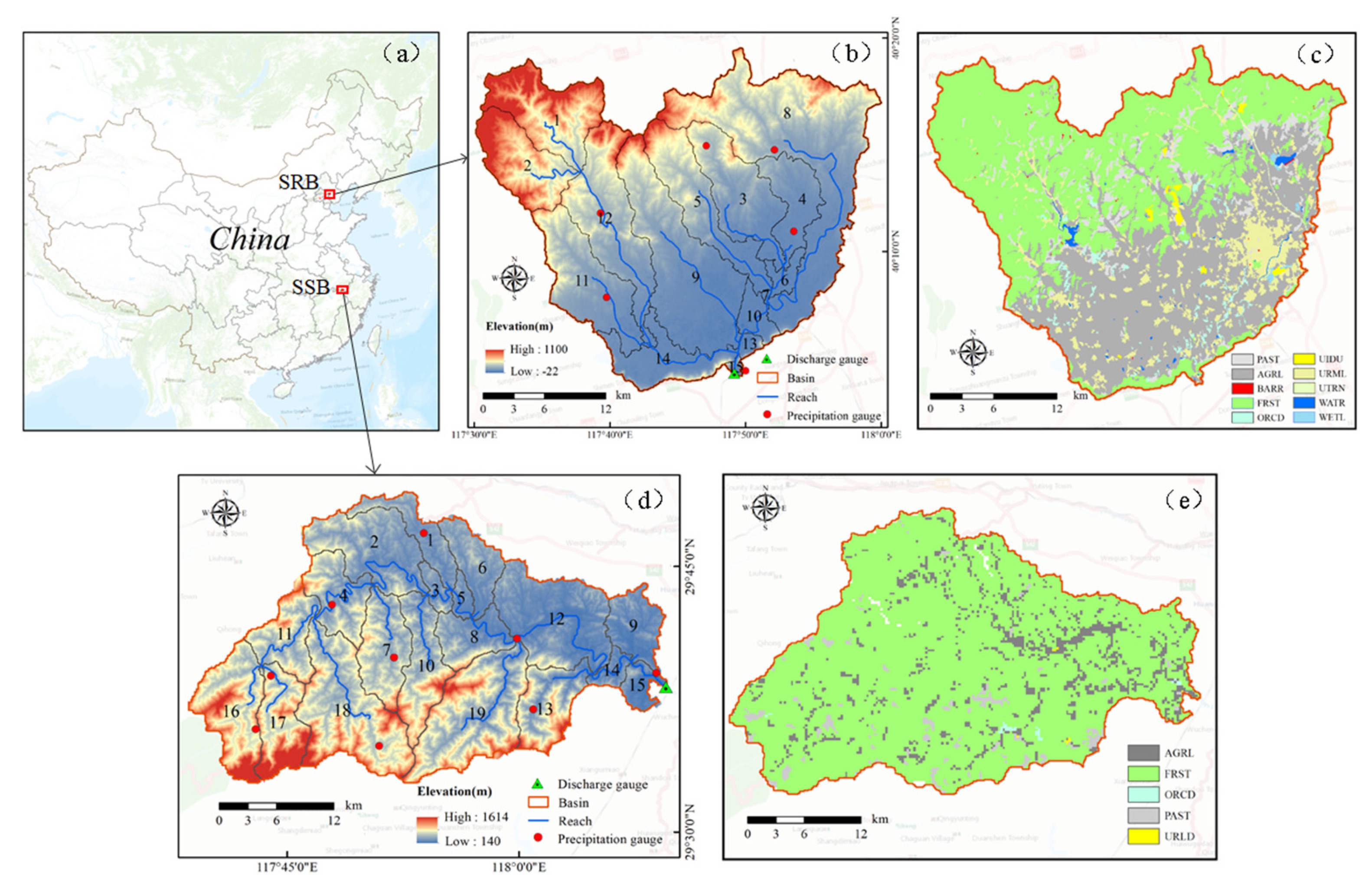
Figure 2.
Schematic diagram of random forest regression model.
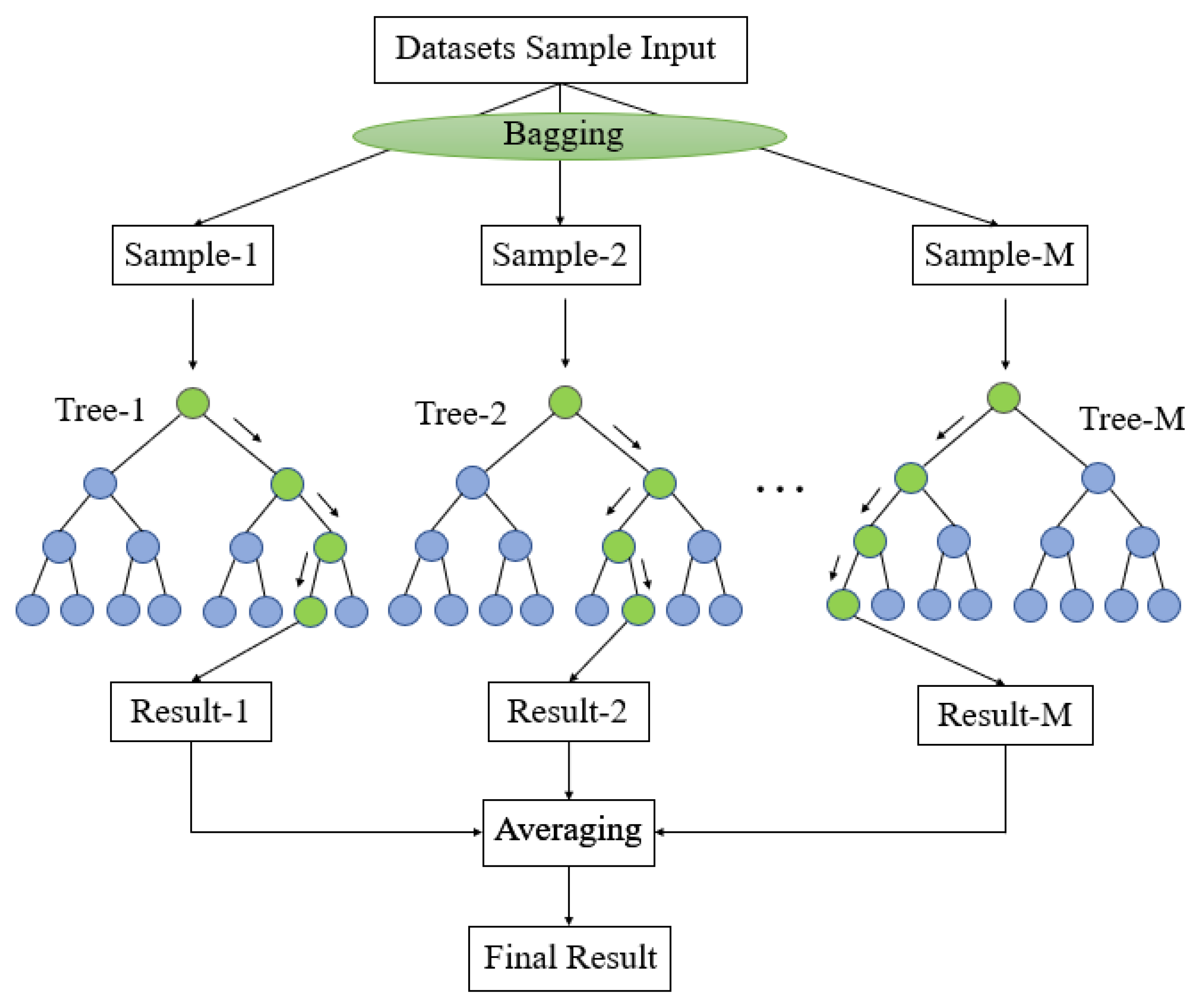
Figure 3.
Comparison of observed and simulated streamflow for SRB using SWAT(a), GWLF(b), and RF(c) model.
Figure 3.
Comparison of observed and simulated streamflow for SRB using SWAT(a), GWLF(b), and RF(c) model.
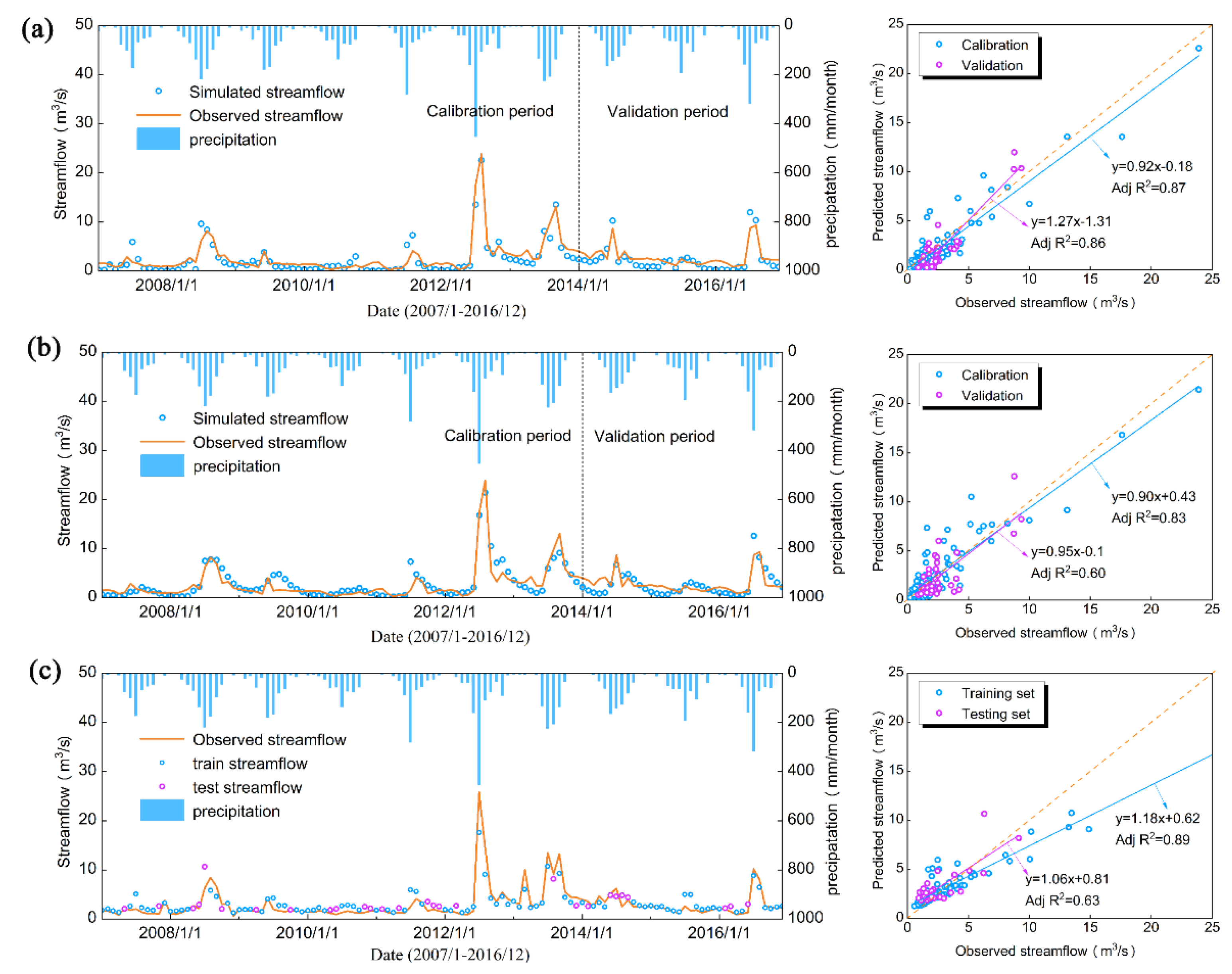
Figure 4.
Comparison of observed and simulated streamflow for SSB using SWAT(a), GWLF(b), and RF(c) model.
Figure 4.
Comparison of observed and simulated streamflow for SSB using SWAT(a), GWLF(b), and RF(c) model.
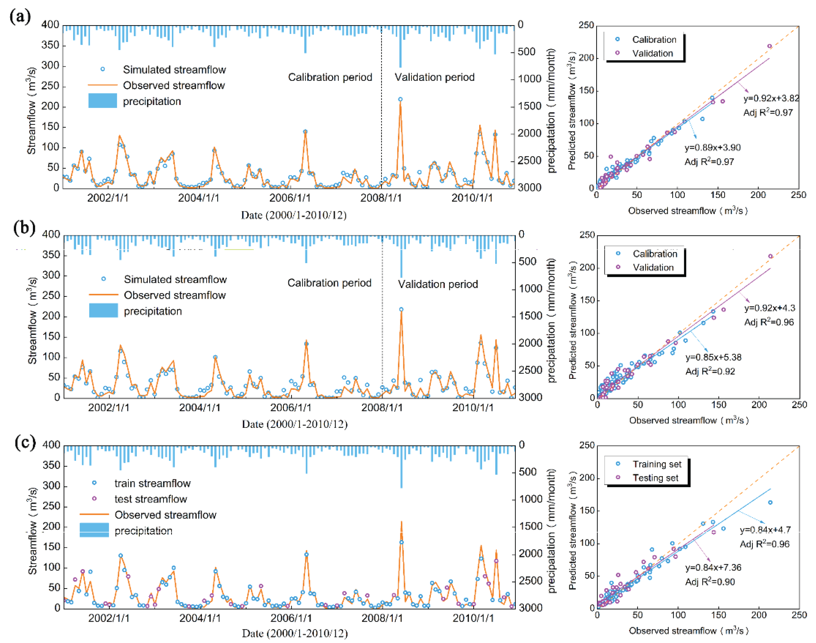
Table 2.
Independent and dependent variable in various scenarios of streamflow simulation.
| Scenarios | Independent variable | Dependent variable |
| I | Pt, ET, AT, RH, WS, SR | Qt |
| II | Pt-1, ET, AT, RH, WS, SR | Qt |
| III | Pt-2, ET, AT, RH, WS, SR | Qt |
| IV | Pt-3, ET, AT, RH, WS, SR | Qt |
Table 3.
Model performance Statistical metrics.
| Statistical metrics | Formula | Range |
| R2 | [0,1] | |
| NSE | [–∞,1] | |
| MAE | [0, ∞] | |
| RMSE | [0, ∞] |
Table 4.
The SWAT and GWLF model parameters selection for calibration in SRB and SSB.
| Model | Parameter | Description | Default value range | Calibrated value | |
| SRB | SSB | ||||
| SWAT | v__CN2.mgt | SCS runoff curve number | 35~98 | 46.47 | 80.06 |
| v__ESCO.hru | Soil evaporation compensation factor | 0~1 | 0.62 | 0.91 | |
| v__SOL_AWC.sol | Available water capacity of the soil layer | 0~1 | 0.88 | 0.36 | |
| v__GW_REVAP.gw | Groundwater “revap” coefficient | 0.02~0.2 | 0.04 | 0.07 | |
| v__GWQMN.gw | Threshold depth of water in the shallow aquifer required for return flow to occur | 0~5000 | 102.5 | 848.87 | |
| v__REVAPMN.gw | Threshold depth of water in the shallow aquifer for “revap” to occur | 0~500 | 210.48 | 373.4 | |
| v__ALPHA_BF.gw | Baseflow alpha factor | 0~1 | 0.59 | 0.88 | |
| v__SOL_K.sol | Saturated hydraulic conductivity | 0~2000 | 23.5 | 10 | |
| v__SFTMP.bsn | Snowfall temperature | -20~20 | 10.59 | 13.4 | |
| v__RCHRG_DP.gw | Deep aquifer percolation fraction | 0~1 | 0.47 | 0.23 | |
| v__LAT_TTIME.hru | Lateral flow travel time | 0~30 | 1.86 | 0.67 | |
| v__SOL_ALB.sol | Moist soil albedo | 0~0.25 | 0.18 | 0.11 | |
| v__SURLAG.bsn | Surface runoff lag coefficient | 0.05~24 | 14.87 | 5.27 | |
| v__SMTMP.bsn | Snowmelt base temperature | -20~20 | 7.03 | 4.28 | |
| v__SOL_BD.sol | Moist bulk density | 0.9~2.5 | 1.57 | 1.74 | |
| GWLF | CN2 | SCS runoff curve number | 0~100 | Varies | Varies |
| (40-100) a | (45-100) a | ||||
| Recess coefficient | Groundwater discharge coefficient | 0.1 | 0.004 | 0.158 | |
| Seepage coefficient | Groundwater seepage constant | 0 | 0.008 | 0.02 | |
| Unsat Avail Wat | Available soil water capacity | - | 14.05 | 9.65 | |
a varies with land use.
Table 5.
The performance metrics of various models and scenarios in SRB and SSB.
| Watershed | Model | Scenario | Model performance metrics Calibration (Validation) | |||
| R2 | NSE | MAE | RMSE | |||
| SRB | SWAT | --- | 0.87 | 0.86 | 1.02 | 1.35 |
| (0.86) | (0.60) | (1.09) | (1.29) | |||
| GWLF | --- | 0.83 | 0.82 | 1.07 | 1.53 | |
| (0.60) | (0.58) | (1.24) | (1.58) | |||
| RF | I | 0.90 | 0.80 | 1.50 | 0.88 | |
| (0.44) | (0.67) | (2.00) | (1.53) | |||
| II | 0.90 | 0.81 | 0.85 | 1.43 | ||
| (0.44) | (0.48) | (1.55) | (2.03) | |||
| III | 0.89 | 0.79 | 0.94 | 1.59 | ||
| (0.63) | (0.66) | (1.06) | (1.36) | |||
| IV | 0.91 | 0.79 | 0.92 | 1.62 | ||
| (0.53) | (0.56) | (1.31) | (1.75) | |||
| SSB | SWAT | --- | 0.97 | 0.97 | 4.08 | 5.72 |
| (0.96) | (0.96) | (6.08) | (9.05) | |||
| GWLF | --- | 0.93 | 0.92 | 6.84 | 8.87 | |
| (0.96) | (0.96) | (7.40) | (9.66) | |||
| RF | I | 0.96 | 0.94 | 5.21 | 8.58 | |
| (0.91) | (0.90) | (7.82) | (10.37) | |||
| II | 0.96 | 0.96 | 4.67 | 8.26 | ||
| (0.85) | (0.89) | (8.69) | (12.68) | |||
| III | 0.97 | 0.96 | 4.44 | 7.65 | ||
| (0.89) | (0.88) | (8.71) | (11.84) | |||
| IV | 0.97 | 0.96 | 4.52 | 7.59 | ||
| (0.90) | (0.89) | (8.53) | (11.33) | |||
Disclaimer/Publisher’s Note: The statements, opinions and data contained in all publications are solely those of the individual author(s) and contributor(s) and not of MDPI and/or the editor(s). MDPI and/or the editor(s) disclaim responsibility for any injury to people or property resulting from any ideas, methods, instructions or products referred to in the content. |
© 2025 by the authors. Licensee MDPI, Basel, Switzerland. This article is an open access article distributed under the terms and conditions of the Creative Commons Attribution (CC BY) license (http://creativecommons.org/licenses/by/4.0/).
Copyright: This open access article is published under a Creative Commons CC BY 4.0 license, which permit the free download, distribution, and reuse, provided that the author and preprint are cited in any reuse.


