Submitted:
13 November 2025
Posted:
14 November 2025
You are already at the latest version
Abstract
The rise of the circular economy and e-commerce has led to the emergence of e-commerce closed-loop supply chains (ECLSC). In practice, investing in process innovation (PI) is key to improving profitability and competitiveness. However, manufacturers at the down-stream of ECLSC often face financial constraints and quality uncertainty of used products, while research on how to select financing strategies under these conditions remains lim-ited. To explore the optimal financing scheme for the ECLSC, this study investigates two financing schemes: bank financing (BF) and FinTech platform financing (FPF), which combines debt financing (DF) and equity financing (EF). Some key findings are derived. For the ECLSC, the FPF scheme is more profitable when the unit manufacturing cost for new components exceeds the threshold or PI costs are relatively low. Additionally, the FPF performs better when consumer sensitivity to recycling prices is high. The BF is more ben-eficial when the FPF scheme's interest rate and DF ratio are relatively high. The FPF ena-bles the ECLSC to achieve maximum profits and minimize environmental impact within a specific range. Furthermore, the financing models are extended to incorporate consider-ations of fairness, in which manufacturing costs primarily influence the optimal financ-ing scheme.
Keywords:
e-commerce closed-loop supply chain
; quality uncertainty
; financing scheme
; fairness concern
1. Introduction
The circular economy (CE) is recognized as an essential strategy for continuously minimizing the environmental harm caused by inefficient production and consumption while helping organizations achieve more resilient ESG (Environmental, Social, and Governance) indicators [1,2]. Closed-loop supply chains (CLSCs), which exemplify the CE in action, have been recognized as a sustainable, low-carbon approach to production [3]. Companies such as Apple, Procter & Gamble, HP, Dell, and Xerox have successfully adopted this approach, reaping significant economic benefits from its implementation[4]. In recent years, the rapid development of e-commerce has attracted a growing number of consumers to shop online and participate in online recycling programs[5]. Thus, E-business has become a crucial component of CE practices worldwide, with some companies transitioning their sales and recycling operations to online platforms, thereby establishing e-commerce closed-loop supply chains (ECLSC). By 2021, around 42,000 e-commerce enterprises in China focused on second-hand products [6].
With price transparency on internet platforms, consumer attention has shifted to services such as logistics, home delivery, and quality inspection, making it essential for platforms to comprehensively assess service levels to stay competitive [7,8]. Moreover, platforms often secure higher profits due to their rule-setting authority and leverage economies of scale, which can lead to fairness concerns (FC) among other members, as seen when the online recycling platform Re-Life shut down due to unfair profit distribution[9]. In this study, we extend our model by incorporating FC to explore its impact further.
In practice, remanufacturing profitability and decision-making are significantly influenced by the quality of used products. Severely damaged products make remanufacturing very challenging or impossible. For instance, Caterpillar Group uses advanced technology to restore unusable core components to like-new conditions, maintaining market competitiveness. However, not all manufacturers have such capabilities, leading to significant uncertainty about the quality of recycled products [10]. Besides, companies that succeed in the remanufacturing sector often invest heavily in process innovation to enhance their capabilities and reduce costs. For instance, Apple's Daisy robot optimizes the disassembly of old products, saving labor and time and lowering remanufacturing costs. Bosch developed a chip to assess the quality of components from its used products. Therefore, this study examines how remanufacturing and ECLSC performance are affected by uncertainty in used product quality, and how remanufacturing enterprises decide on process innovation investment. Furthermore, these factors are often underexplored in other related ECLSC studies [6], highlighting the potential contribution of this research.
Capital constraints are a common challenge for SMEs, driven by pressures such as the need for process innovation and adapting to the evolving regulatory landscape, which increasingly mandates ESG compliance and reporting obligations [11]. Financial institutions provide various solutions to address these funding issues. For example, remanufacturing leader Caterpillar Group secured a $3 billion 9-month revolving credit line from banks [12]. Furthermore, as digital technologies develop, some FinTech platforms offer financing solutions to capital-constrained supply chain participants to support their green and sustainable activities. Platforms like Carbon Chain (https://carbonchain.com) in the UK help SMEs in industries such as metals, oil and gas, mining, and agriculture to reduce carbon emissions and secure green financial support. Overall, FinTech platforms offer several advantages over traditional financing methods. They connect SMEs directly with investors through regulated digital platforms, thus reducing the need for intermediaries and lowering costs. Moreover, these platforms offer diverse financing options, such as debt and equity financing, that help reduce risk for both SMEs and investors. The choice of financing scheme by a capital-constrained manufacturer as a downstream SME in the ECLSC, based on profit performance and environmental impact, is key to balancing economic and sustainability goals, as ESG performance reflected in carbon emissions and energy use is increasingly viewed as a measure of corporate responsibility [13].
Based on the above descriptions and to fill a gap in existing research, this study constructs an ECLSC consisting of an e-commerce platform (E-platform) and a capital-constrained manufacturer under the uncertainty of used product quality. The manufacturer can choose between traditional bank financing (BF) and innovative fintech platform financing (FPF), which combines debt financing (DF) and equity financing (EF) to address the challenge of insufficient funding for process innovation. We aim to explore the following research questions:
- What are the optimal operational decisions and remanufacturing strategies for an ECLSC under scenarios with no financial constraints and different financing schemes, considering the uncertainty in the quality of used products?
- How do the remanufacturing quality threshold and recycling service sensitivity coefficient impact the optimal decisions and profits?
- For the manufacturer facing capital constraints, how should ECLSC choose the appropriate financing scheme? Which financing scheme has a smaller environmental impact?
- If the manufacturer exhibits FC behavior, what impact does FC have on capital-constrained ECLSC?
By addressing the questions outlined above, this study yields several significant findings and contributions.
- We consider the effects of various parameters on the profit of the ECLSC. Our comparative and numerical analyses reveal that the FPF is more favorable when the unit remanufacturing cost exceeds a certain threshold or PI costs are low. The BF is more advantageous when the FPF interest rate and DF ratio are relatively high. Furthermore, when consumer sensitivity to recycling prices is low, the BF is the preferred choice. On the other hand, the FPF scheme remains optimal, regardless of the recycling service sensitivity coefficient. More importantly, the FPF enables the ECLSC to maximize economic benefits while minimizing environmental damage within a specified range. By identifying optimal financing schemes under different conditions, this research provides valuable insights that empower companies to effectively navigate financial constraints, strategically enhance profitability across diverse market environments, and place greater emphasis on minimizing environmental impact.
- Unlike Qin, Chen, Zhang and Ding [10], this study finds that higher remanufacturing quality thresholds reduce recycled product quantities and profits, emphasizing the need for better product design, fostering collaboration, and implementing policy incentives.
- Increased consumer sensitivity to recycling services positively impacts the ECLSC and enables consumers to benefit from higher valuations of used products and improved services under certain conditions. This contrasts with Wang et al. [14], who found it challenging to balance high recycling prices and service levels.
- Manufacturers' FC behavior negatively affects both the recycling efficiency of the ECLSC and the profit of the E-platform. Although FC is often considered harmful to efficiency and profitability [6,15], our findings reveal that within specific ranges, an increase in the FC coefficient can actually lead to higher manufacturer profit. In such cases, the optimal financing scheme selection remains consistent mainly with scenarios without FC, with the influencing factor being the unit manufacturing cost, further validating the robustness of our previous results.
The remainder of this paper is organized as follows: Section 2 reviews the relevant literature. In Section 3 and Section 4, we develop the ECLSC model framework and derive the optimal solutions under different financing schemes. Section 5 analyzes the impact of key parameters and compares the solutions, profits, and environmental effects under the BF and FPF schemes. In Section 6, we conduct numerical analyses to explore further the financing preferences of the overall ECLSC and the manufacturer. In Section 7, we extend the models by considering the FC. Finally, Section 8 makes conclusions and provides corresponding managerial implications. All proofs are included in the Appendix.
2. Literature Review
This section reviews research on online channels in CLSC, consideration of quality in CLSC, PI, and supply chain financing, offering insights that shape this study's approach and direction.
2.1. Online Channels in CLSC
E-commerce has transformed CLSC operations, sparking interest in online and dual-channel models. Kong et al. [16] optimized pricing and service levels to address channel conflicts in dual-channel CLSC networks. Jia and Li [17] analyzed decisions that accounted for platform fees and fulfillment costs. Jin et al. [18] examined channel power structures in reverse supply chains, considering online and offline recycling competition. Wang et al. [19] showed that reward-punishment mechanisms and altruistic preferences enhance the platform's recycling service levels, including quality and quantity. Wang, Yu, Shen and Jin [14] investigated optimal decisions under different sales and recycling models, considering the impact of these models and platform service levels on the CLSC. Cui et al. [20] compared pricing strategies for recycling under extended warranty services on E-platforms. Barman [21] explored different incentive mechanisms to improve the environmental sustainability of eco-friendly products within the closed-loop structure of an ECLSC.
Several studies have explored FC issues from profit gaps between online platforms and other entities. Qin et al. [22] proposed a revenue-sharing contract to address fairness under information symmetry and asymmetry. Wang, Wang, Cheng, Zhou and Gao [6] analyzed consumer preferences for remanufactured and new products and FC. Qin, Wang, Gao and Liu [9] used a signaling model to identify conditions for genuine FC information sharing, reducing profit losses in ECLSCs. Xiao et al. [23] examined the manufacturer's dual behavioral preferences and risk aversion in a dual-channel green supply chain.
Considering the growing importance of CLSCs in the digital economy and the potential challenges they face, this paper examines a fully online ECLSC, focusing on optimizing operations, recycling processes, and financing strategies under capital constraints. Meanwhile, we extend the research scenarios by incorporating FC's perspective. Unlike previous studies that primarily focused on traditional offline or dual-channel CLSCs, or the work of Qin, Wang and Gao [22] and Wang, Wang, Cheng, Zhou and Gao [6] on ECLSC operational model selection and coordination issues, our study provides fresh insights. This research complements the existing CLSC literature and offers practical guidance for ECLSC companies operating under capital constraints.
2.2. The Consideration of Quality in CLSC
Scholars have explored the impact of product quality on consumer preferences and recycling in CLSC. El Saadany and Jaber [24] showed that combining production and remanufacturing is optimal when recycling rates depend on price and quality. Cai et al. [25] studied pricing and production for high and low-quality components. Taleizadeh et al. [26] examined pricing strategies, quality levels, and sales efforts in dual-channel CLSC. Zhang et al. [27] studied pricing, quality, and revenue-sharing for defective and end-of-life products in a dual-channel CLSC. Feng et al. [28] considered competition among new, remanufactured, and refurbished products with subsidies. Qin, Chen, Zhang and Ding [10] examined quality uncertainty in engineering machinery recycling and its impact on remanufacturing decisions. Guo and Chen [29] considered the quality uncertainty of recycled products and explored the scope of government subsidies.
However, most studies assume that homogeneous used products meet remanufacturing standards. Research on the impact of quality uncertainty on recycling efficiency is limited, except for Qin, Chen, Zhang, and Guo and Chen [29]. This study extends the existing literature by examining the effects of both the used product quality uncertainty and recycling efficiency within online recycling channels. Furthermore, we explore the manufacturer's PI activities in response to this quality uncertainty.
2.3. Process Innovation
PI is vital for boosting demand, reducing costs, and improving supply chain performance [30]. Reimann et al. [31] found that PI strategies in forward supply chains do not directly apply to remanufacturing, with high innovation costs favoring decentralized decision-making. Chai et al. [32] studied PI's impact on green product CLSC performance and identified optimal strategies in both cooperative and non-cooperative contexts. Yang, et al. [33] analyzed the role of government subsidies in promoting technological progress. Niu and Shen [34] explored manufacturers' PI decisions under knowledge spillovers and differing absorptive capacities. Pu et al. [35] proposed a dynamic optimal control model that integrates PI and low-carbon efforts within a dual-carbon policy framework, accounting for the impact of knowledge accumulation. Qian et al. [36] explored how upstream and downstream firms determine optimal PI strategies in the context of the interaction between product innovation and PI. They examined how this interaction influences operational decisions.
While existing research emphasizes the PI's role in supply chain sustainability and efficiency, it often assumes firms have sufficient capital, neglecting the significant financial constraints many SMEs face. This study addresses this gap by exploring optimal financing schemes for capital-constrained ECLSC pursuing PI.
2.4. Supply Chain Financing
In recent years, supply chain financing has rapidly developed, addressing SMEs' financing issues and expanding banking services. Several studies have explored various financing models, focusing on their impact on operational decisions[37,38,39,40,41]. Emerging technologies like the internet and cloud computing have introduced new financing methods and platforms. Wang et al. [42] examined how E-platform financing and bank credit affect online retailers. Yi et al. [43] studied agricultural supply chains with small farmers and financing platforms, finding that the platform encourages BF when production costs are high. Reza-Gharehbagh et al. [44] analyzed green product development in SME supply chains using FinTech platforms. Zhang et al. [45] developed a CLSC model for online equity crowdfunding and determined the optimal equity transfer ratio. Verma and Mishra [46] investigate how financing options, such as TCF and BF, improve the sustainability and performance of the CLSC under government subsidies.
Building on previous research, this study compares traditional BF and innovative FPF within ECLSCs. It identifies optimal conditions for each scheme and offers actionable recommendations. Furthermore, we extend the models by incorporating FC considerations. Table 1 summarizes the gaps in existing research and highlights the contributions of this study.
3. Problem Description
Motivated by downstream manufacturers' frequent financial constraints in ECLSCs, this study considers an ECLSC system composed of an E-platform and a risk-neutral, capital-constrained manufacturer (Figure 1), with both parties aiming to maximize profits. The E-platform provides product sales and recycling services and charges commissions for them. The manufacturer sells products and collects used products via the E-platform, remanufacturing those that meet quality standards. To improve efficiency, the manufacturer also invests in PI to reduce remanufacturing costs.
The specific decision sequence is shown in Figure 2. The E-platform, benefiting from economies of scale and rule-making advantages [7], acts as the leader and first decides on the sales commission , the commission for recycling used products , and the platform's recycling service level . Subsequently, the follower manufacturer determines the PI level , the sales price of new products , and the quality-based value coefficient of used products , which in turn determines the recycling price of used products.
Table 2 presents the relevant parameters and their definitions used in this study. To facilitate a deeper analysis of the model, we make the following assumptions:
Assumption 1. The manufacturer sells products via the E-platform, which charges a per-unit commission on sales (This type of fee structure is common in practice, as seen with Amazon) and on recycled products. The E-platform enhances consumer participation in recycling through services like appraisals, inspections, and at-home pickup. These services incur a cost of , where is the service level and the cost coefficient is normalized to 1 [6,14,47].
Assumption 2. Although companies like Apple, Samsung, Huawei, and Amazon actively promote recycling and resale globally, CLSC integration rarely influences consumer behavior or sales [48]. Following related studies, this research assumes products consist of a single component, with new and recycled parts being identical in function and appearance [45,49]. The manufacturer can use new parts at a cost of or remanufacture using recycled parts from used products that exceed the quality threshold , which is more cost-effective (). For simplicity, we set to 0 [50].
Assumption 3. According to Wang, Yu, Shen and Jin [14] and Zhang, Meng and Xie [45], the recycling quantity of used products is , where is the recycling price sensitivity coefficient and is the service level sensitivity coefficient. The recycling price , paid by the manufacturer is expressed as , where is the value coefficient of the used product, and is the quality level. Higher product quality results in a higher recycling price. To simplify, the stochastic variable is assumed to follow a standard uniform distribution based on historical data [10]. The manufacturer remanufactures used products whose quality exceeds the threshold , and for generality, let fixed payment .
Assumption 4. The demand function for the product is , where represents the market size of the product, and represents the sales price sensitivity coefficient [45]. To ensure non-negative results, it is assumed that .
Assumption 5. The manufacturer endeavors to carry out PI activities during the remanufacturing phase, such as improving production processes, implementing technological innovations, and upgrading equipment, which do not involve product design. The PI level is represented by . Through PI, the cost of remanufacturing can be reduced by , while the investment cost is , where is the PI cost coefficient [32,51].
Assumption 6. As SMEs often rely on financing to implement innovative ideas, it is assumed that manufacturers have no restrictions on daily operating capital. In contrast, the capital for process innovation is limited. Specifically, following a similar approach to Xia et al. [52], the manufacturer's loan size is set as to facilitate analysis. The manufacturer can address the funding issue through two schemes: BF and FPF.
4. Model Formulation and Solution
In this section, we develop three models: a benchmark model where the manufacturer faces no financial constraints, the BF model, and the FPF model. We analyze the optimal decisions of the E-platform and the manufacturer under these different scenarios.
4.1. Model Without Capital Constraint (NC)
Given the uncertainty in the quality of used products, the expected profit function of the E-platform is as follows:
Here, the first term represents the commission income from product sales, the second term represents the commission income from recycling used products, and the third term represents the platform's recycling service cost.
Given the uncertainty in the quality of used products, the expected profit function of the manufacturer without financial constraints is as follows:
In Eqn. (2), the first term represents the income from manufacturing using new components, the second term represents the income from remanufacturing, and the third term represents the cost of PI.
Proposition 1.
Given thatand, the optimal solutions under the model where the manufacturer has no financial constraints are as follows: ,,,,,.
The optimal outcomes are summarized in Table 3.
4.2. Bank Financing (BF)
Bank financing, a traditional external financing method, enables the capital-constrained manufacturer to address its funding needs. Some banks also support green innovation financing schemes. For instance, Unilever signed a €500 million sustainability-linked loan agreement with three banks, incorporating its efforts to reduce greenhouse gas emissions, increase renewable energy use, and enhance water management into the agreement conditions[53].
Under the BF scheme, the manufacturer borrows from the bank. At the end of the sales period, the manufacturer is required to repay the bank . The expected profit functions of the E-platform and the manufacturer are as follows:
Proposition 2.
Given thatand, the optimal solutions under the BF model are as follows:,,,,,.
The optimal outcomes are summarized in Table 3.
4.3. FinTech Platform Financing (FPF)
With the advent of FinTech, FinTech-based supply chain finance has emerged as an alternative funding source, enabling SMEs to secure financing through various FinTech platforms. At present, China's FinTech adoption rate is particularly high at 87%, well above the global average of 64%. In the United States, financial innovations such as online lending have proven beneficial for SMEs, offering substantial opportunities for innovation and growth to expand loan availability [54,55]. Moreover, platforms such as CrowdCube and Fundable have become well-known sources of equity crowdfunding, supporting projects in emerging industries such as AI, electronics, and environmental protection [45].
Under the FPF scheme, the FinTech platform allocates funds raised from investors to the supply chain financing project through both DF and EF (Figure 3). The capital-constrained manufacturer obtains from DF and from EF. At the end of the sales period, the manufacturer repays the principal and interest and shares the profits[44].
Given the uncertainty in the quality of used products, the expected profit functions of the E-platform and the manufacturer are as follows:
Proposition 3.
Given thatand, the optimal solutions under the FPF model are as follows: ,,,,,.
The optimal outcomes are summarized in Table 3. Proof of Propositions 1-3: See Appendix A.1.
5. Model Analysis and Comparison
5.1. The Impact of Key Parameters
Corollary 1.
The impact of the remanufacturing quality thresholdon optimal decisions and profits is as follows:,,,; ifand, then, otherwise; ifand, then, otherwise; ifand, then, otherwise. ,,;,.
Corollary 1 suggests that raising the quality threshold reduces recycling services, recycling commissions, PI, and the quantity of recycled products, contrary to Qin, Chen, Zhang,. A higher threshold makes recycling less attractive for ECLSC companies as remanufacturing becomes costlier and less profitable. However, an increased threshold does not always lower the manufacturer's valuation of used products. Only when recycling price sensitivity is high and PI costs are low does a higher threshold reduce the value coefficient for used products. Otherwise, manufacturers may increase this coefficient to balance recyclable supply and optimize decisions. Additionally, sales commissions, prices, and overall sales volumes remain unaffected by the quality threshold, despite changes in recycling and remanufacturing. Finally, a higher remanufacturing threshold lowers profits for ECLSC members, making remanufacturing less economically viable. To address this, companies could collaborate with advanced remanufacturers or adopt recycling-friendly product designs [56].
Corollary 2.
The impact of the recycling service level sensitivity coefficient ϕ on the optimal decisions and profits is as follows:,,,. When, if, then, otherwise; if, then, otherwise; if, then, otherwise.When, then. ,,;,.
Corollary 2 shows that as consumers value recycling services more, the E-platform invests in better services to boost participation. Despite rising costs, increased recycling commissions and quantities make recycling more profitable. For the manufacturer, higher volumes of used products enhance remanufacturing benefits, encouraging greater PI investment.
Furthermore, when recycling price sensitivity is high and the PI cost coefficient is low, the manufacturer raises the valuation of used products to attract consumers, increasing income from PI. Consumers benefit from higher recycling prices and improved services, unlike findings by Wang, Yu, Shen and Jin [14], where both were not achievable simultaneously. In reality, Luxury resale platforms like The RealReal and Vestiaire Collective exemplify this by enhancing services (e.g., free authentication, home pick-up) to attract high-end consumers [57]. Conversely, if PI costs are high or recycling price sensitivity is low, the manufacturer will reduce valuations to manage costs. Moreover, the recycling service sensitivity coefficient mainly affects the ECLSC recycling segment, indicating that greater consumer emphasis on recycling services enhances ECLSC efficiency, improves remanufacturing profitability, and benefits both the e-commerce platform and the manufacturer.
Finally, through Corollary 1 and Corollary 2, we find that the impacts of the remanufacturing quality threshold and the recycling service coefficient are not influenced by the presence of financial constraints or differences in financing schemes.
Proof of Corollaries 1-2: SeeAppendix A.2.
5.2. Comparison Between BF and FPF Schemes
To ensure that all financing schemes have optimal solutions and to avoid trivial cases, it is assumed that in the following subsections. Based on Proposition 2 and Proposition 3, we compared two financing schemes and obtained the following conclusions.
5.2.1. The Optimal Decisions
Corollary 3.
In the case oforand, there exist,,,;if, then, otherwise,. In the case of, whenthere exist,,,; if, then, otherwise,.
According to Corollary 3, when the bank interest rate is greater than or equal to the FPF interest rate, or when the FPF interest rate is higher and the DF ratio is less than or equal to the threshold, the FPF results in higher recycling service levels, recycling commissions, and greater manufacturer investment in PI. However, for the valuation of used products, when the recycling price sensitivity coefficient is low, the manufacturer under the BF tends to set higher valuations to attract consumers and mitigate the higher financing costs of PI capital. Nevertheless, the quantity of used products under the FPF remains higher than that under the BF scheme. When the FPF interest rate is higher and the DF ratio exceeds the threshold, the comparison results are opposite to the above findings. In this scenario, the manufacturer is more motivated to implement recycling, remanufacturing, and PI under the BF. At the same time, the E-platform is more inclined to provide higher levels of recycling services.
Corollary 4. ,,.
As shown in Corollary 4, different PI capital financing schemes in this study do not affect the forward logistics channels. Similar to the results of Chai, Qian, Wang and Zhu [32], the total product sales remain unchanged, allowing us to better investigate the impact of financing schemes on remanufacturing performance and recycling efficiency.
5.2.2. The Profit Performance
To facilitate the comparison of the profit of ECLSC, in Corollary 5, we assume , , , and . Considering corporate control in EF under the FPF, we assume .
Corollary 5.
If, then, otherwise,. Theis positively correlated with. whereis placed in theAppendix C.
According to Corollary 5, when the unit manufacturing cost exceeds a certain threshold (), meaning that the cost of producing products using entirely new components is relatively high, the profit of the ECLSC is higher under the FPF. This is because higher unit manufacturing costs indicate that the manufacturer relies more heavily on remanufactured products and must invest significantly in PI. Since PI often requires substantial financial resources, the FPF, which provides a flexible combination of DF and EF, becomes more advantageous. For instance, companies like Apple Inc and Tesla, which invest in advanced manufacturing technologies and relieve on continuous innovation, might find the FPF beneficial as it offers flexible financing options to support innovation. In contrast, when the unit manufacturing cost is below this threshold (), the BF yields higher profit. In this scenario, the lower reliance on remanufacturing and PI makes traditional BF more suitable. Companies in the fast-moving consumer goods sector may find the BF more advantageous for maintaining profitability without the need for extensive innovation financing.
Furthermore, the remanufacturing quality threshold positively influences the unit manufacturing cost threshold, indicating that as the remanufacturing quality threshold increases, the cost threshold at which the FPF becomes more advantageous also rises. In practice, when higher standards are set for the quality of used products, such as in the luxury goods industry where strict conditions are required for recycled items, the benefits of the FPF may diminish. Thus, ECLSC companies might need to weigh the potential benefits of FPF against the increasing quality threshold to determine the most effective financing strategy.
5.2.3. The Profit Performance
Although financial returns remain a critical measure of success in the private sector, core companies like Walmart and Carrefour prioritize building green supply chains by setting environmental standards for their suppliers, who risk losing their contracts if they fail to meet these criteria [58]. Therefore, it is essential to analyze the environmental impact (EI) under different schemes. We use the EI index to compare the environmental effects under different financing schemes [59]. Previous studies [60] show that remanufacturing consumes 20-60% less energy than producing new products. The function for calculating the EI index is . For simplicity, we normalize to 1, while is set to 1/2. By substituting equilibrium results, the following outcomes and Corollaries are derived.
Corollary 6.
Iforand,then; ifand,then,.
Corollary 6 indicates that when the BF interest rate is greater than or equal to the FPF interest rate, or when the FPF interest rate is higher and the DF ratio is less than or equal to the threshold, the EI under the BF is higher than that under the FPF. Combined with Corollary 3, this outcome suggests that the lower recycling efficiency of the ECLSC under the BF forces manufacturers rely more heavily on new components in production, leading to significantly increased environmental damage.
Substituting the parameter values from Corollary 5 (i.e., , , , , , ), we observe that the EI under the FPF scheme is consistently lower than that under the BF scheme. Specifically, when , opting for the FPF scheme enables the simultaneous achievement of maximum economic benefits and minimized environmental damage for the ECLSC. Aligning financing decisions with sustainability objectives through such strategies can enhance overall performance. Furthermore, this finding suggests that socially responsible manufacturing companies operating under the BF scheme must place greater emphasis on investing in carbon reduction, green innovation, and other sustainable practices to reduce their EI effectively.
6. Numerical Analysis
This section utilizes numerical examples to further analyze the profit comparison of the profit of ECLSC. The numerical examples are sourced from Wang, Yu, Shen and Jin [14], with certain values adjusted to align with the conditions of this study's model. We set the bank interest rate , in line with the benchmark annual interest rate for short-term loans in China. The remaining settings are as follows: the market size the market size , the sales price sensitivity coefficient .
6.1. The Combined Impact of Unit Cost of Manufacturing and Quality Threshold
Assume that , , , , and . By setting and , we use two sets of parameters (viz., and ) to plot the changes in the profit of the ECLSC with the unit cost of manufacturing and the quality threshold in Figure 4.
Figure 4 illustrates that in region 1 (i.e., the left side of the dashed line), when is relatively high and is relatively low, which are conditions favorable for remanufacturing, choosing the FPF results in higher overall profit for the ECLSC. As increase, the profit under the FPF remains consistently higher in region 2 (i.e., the right side of the dashed line). Moreover, it is noteworthy that the relationship between the interest rates of the two financing schemes does not affect the choice of the optimal financing scheme currently.
6.2. The Combined Impact of FinTech Platform Interest Rate and Debt Financing Ratio
Assuming that , , , , , and after we set and , the combined impact of and is illustrated in Figure 5.
Figure 5 shows that when both and are relatively high, the ECLSC profit is greater under the BF. Combined with Corollary 3, this indicates that the BF achieves higher recycling efficiency and PI levels in this situation. Otherwise, the FPF becomes the preferable choice.
6.3. The Impact of Relevant Parameters
This section explores the key parameters such as the PI cost coefficient , the recycling price sensitivity coefficient , and the recycling service sensitivity coefficient gamma, which influence the ECLSC profit. The specific parameter settings are detailed in Table 4.
Fig. 6 illustrates the impact of on the difference in profits of ECLSC between the two financing schemes. As shown in Fig. 6, when is low, the profit under the BF scheme is lower than under the FPF. However, as increases, the profit under the BF surpasses that of the FPF. Combining these findings with those from Section 6.1, we conclude that in scenarios favorable to remanufacturing, the ECLSC can achieve higher profits under the FPF. These results suggest that the ECLSC company needs to carefully evaluate its PI costs and ensure strategic alignment with industry conditions before selecting a financing option.
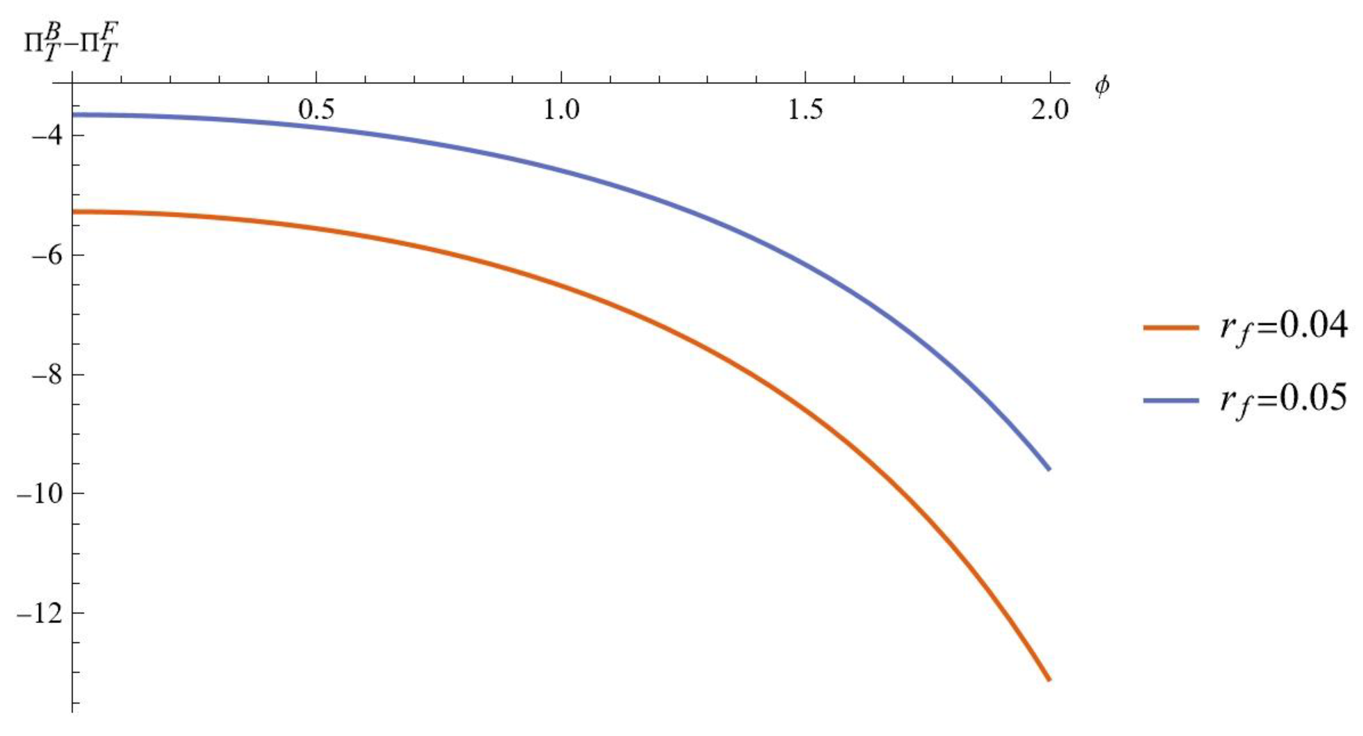
Fig. 7 shows that when is low, the ECLSC profit is greater under the BF. When is high, the FPF results in higher profit. Interestingly, Fig. 8 reveals that does not significantly impact the profit difference of the ECLSC. In fact, the profit under the FPF consistently surpasses that of the BF, regardless of the recycling service sensitivity coefficient.
Overall, understanding and anticipating market condition changes related to recycling price and service sensitivity can lead to more informed and effective financing decisions, ultimately enhancing the sustainability and profitability of the ECLSC.
Figure 6.
Impact of on ( and ).
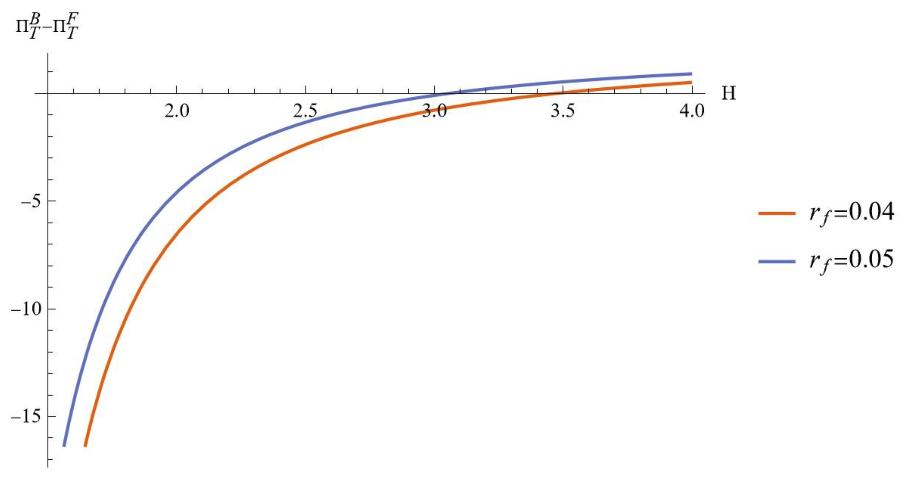
Figure 7.
Impact of on ( and ).
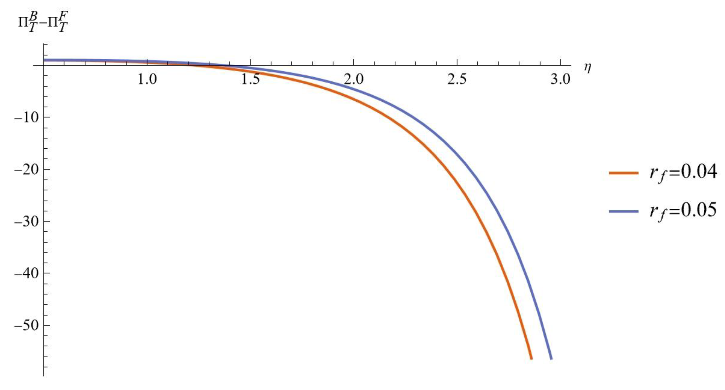
Figure 8.
Impact of on ( and ).
7. Model Extension: Decision Making with Fairness Concern
In practice, stakeholders may act against their own interests to address perceived unfairness and seek more equitable outcomes [61]. Manufacturers often face profit gaps due to the economies of scale of E-platforms, raising concerns about fair profit distribution [6]. Therefore, this section incorporates the fairness concerns (FC) behavior of the manufacturer into decision-making. According to Wang, Wang, Cheng, Zhou and Gao [6], the utility function of the manufacturer with FC defined as follows.
We focus on a single manufacturer to clearly capture the core interaction with the E-platform, even though most platforms engage with multiple manufacturers in practice. Therefore, comparing directly the income gap between the two parties in this section is inappropriate. It is necessary to introduce a relative fairness reference point, represented by . In Eqn. (9), denotes the manufacturer's FC coefficient, reflecting the decrease in the manufacturer’s utility when its profit is less than .
In this scenario, the manufacturer makes decisions based on utility maximization, while the E-platform continues to focus on profit maximization. The optimal outcomes and the conditions that need to be satisfied are summarized in Table 5.
From the Table 5, it is evident that when , the optimal solutions of the models with FC are consistent with those of the models without FC. Regardless of the financing scheme, the FC coefficient consistently affects the optimal solutions and profits in the same direction.
Corollary 7.
The impact of the FC coefficienton optimal decisions is as follows:,,,; if, then, otherwise; ifand, then, otherwise; ifand, then, otherwise. ,,.
Corollary 7 reveals that when manufacturers are concerned about fairness, an increase in the FC coefficient leads the E-platform to reduce the recycling service level, recycling commission, and sales commission in an attempt to mitigate the impact of the manufacturer's FC. Simultaneously, the manufacturer's focus on fairness weakens its incentive to invest in PI. It is worth noting that the impact of the FC coefficient on the valuation of used products depends on specific conditions involving the recycling price sensitivity coefficient and the PI cost coefficient. Under certain conditions, an increase in fairness concerns might unexpectedly lead to higher product valuations, reflecting the manufacturer’s flexible pricing strategy aimed at reducing the profit gap. It is also observed that this range differs between the capital-unconstrained and financing models. These changes consequently have a negative impact on the recycling efficiency of the ECLSC.
Corollary 8.
The impact of the FC coefficienton profits is as follows:; The impact ofonis not linear, e.g., ifand,then; ifand,then; ifand, then.
Corollary 8 shows that the manufacturer’s focus on the profit gap results in a decrease in the E-platform’s profit, but the effect on the manufacturer’s profit is complex and non-linear. While FC are generally perceived as detrimental to efficiency and economic profit[6,15], within a certain range, they can encourage the manufacturer to adjust its decisions, potentially increasing the manufacturer’s profit.
Due to the complicated profit results, we compare the ECLSC profit by applying the numerical values from Corollary 5 that also satisfy the optimal solution conditions under models with FC and referencing Wang, Wang, Cheng, Zhou and Gao [6], assuming and .
Corollary 9. If the unit manufacturing cost satisfies , then , otherwise . Among them, can be found in Appendix D.
According to Corollary 9, when the manufacturer exhibits FC behavior, the ECLSC profit under different financing schemes, similar to the results of Corollary 5, is influenced by the unit manufacturing cost. When the unit manufacturing cost falls within a certain range, the ECLSC profit under the BF is higher than that under the FPF. Our analysis further confirms the robustness of these findings, demonstrating that the financing scheme's impact on profitability is consistent across different scenarios. This emphasizes the importance of carefully considering cost structures when choosing the optimal financing strategy, especially in the presence of FC.
Proof of Corollaries 7-9: SeeAppendix A.4.
8. Conclusions and Management Implications
This study constructs an ECLSC with an E-platform and a capital-constrained manufacturer, considering uncertainties in used product quality, PI, and FC. It examines optimal decisions under different financing schemes, analyzes the effects of remanufacturing quality thresholds and recycling service sensitivity on decisions and profits, and identifies the best financing scheme through comparative and numerical analyses. Additionally, it compares EI as a CE performance metric and explores the impact of the manufacturer's FC on decisions and financing strategies. Based on both analytical and numerical studies, we derived the following major findings and their respective implications.
First, for capital-constrained ECLSC, financing scheme selection depends on various factors, which extends the findings of [44].
- The FPF scheme is ideal when the unit remanufacturing cost exceeds the threshold , which correlates positively with the remanufacturing quality threshold. Therefore, it is recommended that enterprises establish cooperative mechanisms with FinTech platforms and integrate them with their ERP and inventory management systems to provide real-time insights into various operational data, facilitate accurate cost tracking, and jointly develop appropriate financing strategies. FPF is also preferable when PI cost is low, making it suitable for industries like fast moving consumer goods, and luxury industry, where manufacturing is mature and profitable.
- Attention should be given to the financing interest rate and DF ratio. When the FPF scheme's interest rate is higher than that of the BF and the DF ratio is relatively high, the BF becomes the preferred option due to its ability to achieve higher recycling efficiency and improved PI levels within the ECLSC. To address this, FinTech platforms might consider setting more competitive interest rates and thoughtfully balancing the proportions of DF and EF. This approach could help ensure that their financing offerings continue to appeal to companies seeking to optimize their ECLSC operations.
- Low consumer sensitivity to recycling prices favors BF, while recycling service sensitivity has minimal impact, keeping FPF as the optimal choice. The growing importance of consumers in the e-commerce economy is undeniable. JD.com, a leading Chinese e-commerce company, utilizes cloud computing and big data to analyze consumer behavior and preferences, enriching user profiles and supporting its financial services. E-platforms should leverage their data processing and computational strengths to further support ECLSC financing.
Second, the BF increases environmental impact, especially when its interest rate is comparable to or higher than the FPF rate, or when the FPF rate is higher but the DF ratio is low. This is due to lower recycling efficiency, requiring more new components. In contrast, the FPF scheme consistently reduces environmental impact within a specific range, balancing economic gains with environmental benefits. Manufacturers using the BF scheme should focus on carbon reduction, green innovation, and sustainable practices to minimize their environmental footprint.
Third, a higher remanufacturing quality threshold reduces recycled product volume in the ECLSC, diminishing remanufacturing profitability and overall ECLSC profits. Notably, this threshold only lowers the manufacturer's valuation of used products when the recycling price sensitivity is high, and PI cost is low; otherwise, the manufacturer increases the valuation to optimize recycling. To address these challenges, manufacturers can enhance product design and collaborate with advanced remanufacturers. Policymakers can also offer incentives, such as China's subsidies for recycling WEEE and EV batteries, to promote recycling and technological upgrades [62,63].
Moreover, higher consumer sensitivity to E-platform recycling services positively impacts the ECLSC, benefiting consumers through better services, encouraging manufacturers to recycle and invest in PI, and boosting ECLSC profits. Unlike Wang, Yu, Shen and Jin [14], who found improved services could lower recycling prices, this study shows that high consumer sensitivity to recycling prices combined with low cost of PI allows consumers to benefit from higher valuations of used products. This highlights the need for E-platforms to enhance consumer sensitivity through marketing, surveys, and promotions.
Finally, manufacturers' FC behavior reduces ECLSC recycling efficiency and E-platform profits, highlighting the need for fair profit-sharing rules and regulatory oversight. Interestingly, within certain ranges of recycling price sensitivity and PI cost, manufacturers' profits may increase with higher FC coefficients. In such cases, the optimal financing scheme remains largely determined by unit manufacturing costs, similar to scenarios without FC.
However, this study has several limitations that future research could address. First, it assumes a linear product demand function and future work could explore the effects of demand uncertainty on ECLSC. Second, financing interest rates and ratios are treated as fixed parameters. Future studies could model financial institutions' decision-making to analyze their impact on ECLSC financing preferences. Finally, the model could be extended to more complex scenarios, such as multi-enterprise competition or government intervention.
Author Contributions
Conceptualization, J.C. and H.T.; methodology, J.C., Y.T. and H.T.; formal analysis, J.C. and C.P.; writing—original draft preparation, J.C.; writing—review and editing, Y.T., C.P. and H.T; supervision, Y.T., C.P. and H.T.; project administration, Y.T. and H.T. All authors have read and agreed to the published version of the manuscript.
Institutional Review Board Statement
Not applicable.
Informed Consent Statement
Not applicable.
Data Availability Statement
The original contributions presented in this study are included in the article. Further inquiries can be directed to the first author.
Acknowledgments
This research was supported by the Guangdong Province Key Research Base of Humanities and Social Sciences (Grant No. 2022WZJD012).
Conflicts of Interest
The authors declare no conflicts of interest.
Abbreviations
The following abbreviations are used in this manuscript:
| ECLSC | E-commerce closed-loop supply chain (ECLSC) |
| CLSC | Closed-loop supply chain |
| PI | Process innovation |
| BF | Bank financing |
| FPF | FinTech platform financing |
| DF | Debt financing |
| EF | Equity financing |
| FC | Fairness concerns |
Appendix A
Appendix A.1. Proof of Propositions 1-3
Propositions 1
The Hessian matrix of with respect to , and can be solved as follows: . When , is a negative definite matrix. Solving the first order condition of yields: , , . Substitutes those into Eqn. (1), then obtains the Hessian matrix of with respect to , and ,. When and , is a negative definite matrix. Solving the first order condition of Eqn. (1) yields , and . Substituting these solutions into , and derives , and .
Propositions 2
The Hessian matrix of with respect to , and can be solved as follows: . When , is a negative definite matrix. Solving the first order condition of yields: , , . Substitutes those into Eqn. (1), then obtains the Hessian matrix of with respect to , and ,. When and , is a negative definite matrix. Solving the first order condition of Eqn. (3) yields , and . Substituting these solutions into , and derives , and .
Propositions 3
The Hessian matrix of with respect to , and can be solved as follows: . When , is a negative definite matrix. Solving the first order condition of yields: , , . Substitutes those into Eqn. (5), then obtains the Hessian matrix of with respect to , and ,. When and , is a negative definite matrix. Solving the first order condition of Eqn. (5) yields , and . Substituting these solutions into , and derives , and .
Appendix A.2. Proof of Corollaries 1-2
Corollary 1 We present the proof under the FPF scheme, and the proofs for other models follow a similar procedure and are therefore omitted.
,,,; , ifand, then, otherwise . ,.
Corollary 2 We present the proof under the FPF scheme, and the proofs for other models follow a similar procedure and are therefore omitted.
, , , . .When, if, then, otherwise.When, then. ,.
Appendix A.3. Proof of Corollaries 3-6
Corollary3
,
,
,
,
. In the case oforand, there exist,,,;if, then, otherwise,. In the case of, whenthere exist,,,; if, then, otherwise,.
Corollary4
,,Corollary5
, if, then, otherwise,. where,,
,
,
,
,
Corollary6
, iforand,then; ifand,then,.
Appendix A.4. Proof of Model Extension
We present the proof under the FPF scheme, and the proofs for other models follow a similar procedure and are therefore omitted.
The Hessian matrix of with respect to , and can be solved as follows: . When , is a negative definite matrix. Solving the first order condition of yields: , , . Substitutes those into , then obtains the Hessian matrix of with respect to , and ,. When and , is a negative definite matrix. Solving the first order condition of yields , and . Substituting these solutions into , and derives , and .
Corollary7.
,,,,.
, if and , then , otherwise .
Corollary8.
;, where , if and , then .
Corollary9
, where.
If the unit manufacturing cost satisfies , then , otherwise . , where, .
References
- Fatimah, Yun Arifatul, Devika Kannan, Kannan Govindan, and Zainal Arifin Hasibuan. Circular Economy E-Business Model Portfolio Development for E-Business Applications: Impacts on Esg and Sustainability Performance. Journal of Cleaner Production 2023, 415, 137528. [CrossRef]
- Wamane, Gopal Vasudeo. A “New Deal” for a Sustainable Future: Enhancing Circular Economy by Employing Esg Principles and Biomimicry for Efficiency. Management of Environmental Quality: An International Journal 2023, 36, 930–47. [Google Scholar] [CrossRef]
- Gong, Bengang, Zihao Li, Jinshi Cheng, and Xiaoqi Zhang. Closed-Loop Supply Chain Decisions Considering Carbon Tax Policy under the Recycler’s Risk Aversion. Annals of Operations Research, 2025.
- Zheng, Benrong, Kun Wen, Liang Jin, and Xianpei Hong. Alliance or Cost-Sharing? Recycling Cooperation Mode Selection in a Closed-Loop Supply Chain. Sustainable Production and Consumption 2022, 32, 942–55. [Google Scholar] [CrossRef]
- Sun, Zijiao, and Jun Tu. Research on Coordination of the E-Commerce Platform Supply Chain Considering Tripartite Ai Investments. Journal of Theoretical and Applied Electronic Commerce Research, 2025; 20.
- Wang, Yuyan, Dexia Wang, T. C. E. Cheng, Rui Zhou, and Junhong Gao. Decision and Coordination of E-Commerce Closed-Loop Supply Chains with Fairness Concern. Transportation Research Part E: Logistics and Transportation Review 2023, 173, 103092. [CrossRef]
- Siddiqui, Atiq W., and Syed Arshad Raza. Electronic Supply Chains: Status & Perspective. Computers & Industrial Engineering 2015, 88, 536–56.
- Shen, Bin, Rongrong Qian, and Tsan-Ming Choi. Selling Luxury Fashion Online with Social Influences Considerations: Demand Changes and Supply Chain Coordination. International Journal of Production Economics 2017, 185, 89–99. [CrossRef]
- Qin, Yanhong, Shaojie Wang, Neng Gao, and Guirong Liu. The Signaling Mechanism of Fairness Concern in E-Clsc. Journal of Organizational and End User Computing 2023, 35, 1–35.
- Qin, Lin, Weida Chen, Yongming Zhang, and Junfei Ding. Cooperation or Competition? The Remanufacturing Strategy with Quality Uncertainty in Construction Machinery Industry. Computers & Industrial Engineering 2023, 178, 109106.
- Baid, Vaishali, and Vaidyanathan Jayaraman. Amplifying and Promoting the “S” in Esg Investing: The Case for Social Responsibility in Supply Chain Financing. Managerial Finance 2022, 48, 1279–97. [CrossRef]
- Ma, Peng, and Yue Meng. Optimal Financing Strategies of a Dual-Channel Closed-Loop Supply Chain. Electronic Commerce Research and Applications 2022, 53, 101140. [CrossRef]
- Zeng, Huiling, Rita Yi Man Li, and Liyun Zeng. Evaluating Green Supply Chain Performance Based on Esg and Financial Indicators. Frontiers in Environmental Science 2022, 10, 982828. [CrossRef]
- Wang, Yuyan, Zhaoqing Yu, Liang Shen, and Mingzhou Jin. Operational Modes of E-Closed Loop Supply Chain Considering Platforms’ Services. International Journal of Production Economics, 2022; 251.
- Wang, Yuyan, Mei Su, Liang Shen, and Rongyun Tang. Decision-Making of Closed-Loop Supply Chain under Corporate Social Responsibility and Fairness Concerns. Journal of Cleaner Production 2021, 284, 125373. [CrossRef]
- Kong, Lingcheng, Zhiyang Liu, Yafei Pan, Jiaping Xie, and Guang Yang. Pricing and Service Decision of Dual-Channel Operations in an O2o Closed-Loop Supply Chain. Industrial Management & Data Systems 2017, 117, 1567–88.
- Jia, Dongfeng, and Sijie Li. Optimal Decisions and Distribution Channel Choice of Closed-Loop Supply Chain When E-Retailer Offers Online Marketplace. Journal of Cleaner Production 2020, 265, 121767. [CrossRef]
- Jin, Liang, Benrong Zheng, and Shoujun Huang. Pricing and Coordination in a Reverse Supply Chain with Online and Offline Recycling Channels: A Power Perspective. Journal of Cleaner Production 2021, 298, 126786. [CrossRef]
- Wang, Yuyan, Zhaoqing Yu, Liang Shen, and Wenquan Dong. Impacts of Altruistic Preference and Reward-Penalty Mechanism on Decisions of E-Commerce Closed-Loop Supply Chain. Journal of Cleaner Production 2021, 315, 128132. [CrossRef]
- Cui, Xin, Chi Zhou, Jing Yu, and Ali Nawaz Khan. Interaction between Manufacturer’s Recycling Strategy and E-Commerce Platform’s Extended Warranty Service. Journal of Cleaner Production 2023, 399, 136659. [CrossRef]
- Barman, Abhijit. Pricing and Greening Decision in E-Commerce Supply Chain: A Strategic Analysis of Exchange Facility & Refund Policy under Sustainable Manufacturing. Electronic Commerce Research, 2025.
- Qin, Yanhong, Shaojie Wang, and Neng Gao. Coordination Mechanism of E-Closed-Loop Supply Chain under Social Preference. Sustainability, 2022; 14.
- Xiao, Qiang, Zongyan Gao, Qiyuan Zhang, and Zhixin Xia. Pricing Policies of Dual-Channel Green Supply Chain: Considering Manufacturers’ Dual Behavioural Preferences and Government Subsidies. International Journal of Systems Science: Operations & Logistics, 2024; 11.
- El Saadany, Ahmed M. A., and Mohamad Y. Jaber. A Production/Remanufacturing Inventory Model with Price and Quality Dependant Return Rate. Computers & Industrial Engineering 2010, 58, 352–62. [Google Scholar]
- Cai, Xiaoqiang, Minghui Lai, Xiang Li, Yongjian Li, and Xianyi Wu. Optimal Acquisition and Production Policy in a Hybrid Manufacturing/Remanufacturing System with Core Acquisition at Different Quality Levels. European Journal of Operational Research 2014, 233, 374–82. [Google Scholar] [CrossRef]
- Taleizadeh, Ata Allah, Mohammad Sadegh Moshtagh, and Ilkyeong Moon. Pricing, Product Quality, and Collection Optimization in a Decentralized Closed-Loop Supply Chain with Different Channel Structures: Game Theoretical Approach. Journal of Cleaner Production 2018, 189, 406–31. [Google Scholar] [CrossRef]
- Zhang, Zhe, Sen Liu, and Ben Niu. Coordination Mechanism of Dual-Channel Closed-Loop Supply Chains Considering Product Quality and Return. Journal of Cleaner Production 2020, 248, 119273. [Google Scholar] [CrossRef]
- Feng, Dingzhong, Chao Shen, and Zhi Pei. Production Decisions of a Closed-Loop Supply Chain Considering Remanufacturing and Refurbishing under Government Subsidy. Sustainable Production and Consumption 2021, 27, 2058–74. [Google Scholar] [CrossRef]
- Guo, Jianquan, and Lian Chen. Configuration and Optimisation of a Green Closed-Loop Supply Chain with Delivery Time and Green Investment Considering Government Subsidy under Meta-Heuristics Algorithms. International Journal of Systems Science: Operations & Logistics, 2024; 11.
- Zimmermann, Ricardo, Luís Miguel D. F. Ferreira, and Antonio Carrizo Moreira. The Influence of Supply Chain on the Innovation Process: A Systematic Literature Review. Supply Chain Management: An International Journal 2016, 21, 289–304. [Google Scholar] [CrossRef]
- Reimann, Marc, Yu Xiong, and Yu Zhou. Managing a Closed-Loop Supply Chain with Process Innovation for Remanufacturing. European Journal of Operational Research 2019, 276, 510–18. [Google Scholar] [CrossRef]
- Chai, Junwu, Zhifeng Qian, Feng Wang, and Jing Zhu. Process Innovation for Green Product in a Closed Loop Supply Chain with Remanufacturing. Annals of Operations Research 2021.
- Yang, Rui, Wansheng Tang, and Jianxiong Zhang. Technology Improvement Strategy for Green Products under Competition: The Role of Government Subsidy. European Journal of Operational Research 2021, 289, 553–68. [Google Scholar] [CrossRef]
- Niu, Wenju, and Houcai Shen. Investment in Process Innovation in Supply Chains with Knowledge Spillovers under Innovation Uncertainty. European Journal of Operational Research 2022, 302, 1128–41. [Google Scholar] [CrossRef]
- Pu, Han, Xinping Wang, Tiezhi Li, and Chang Su. Dynamic Control of Low-Carbon Efforts and Process Innovation Considering Knowledge Accumulation under Dual-Carbon Policies. Computers & Industrial Engineering 2024, 196, 110526. [Google Scholar]
- Qian, Zhifeng, Joshua Ignatius, Junwu Chai, and Krishna Mohan Thazhathu Valiyaveettil. To Cooperate or Not: Evaluating Process Innovation Strategies in Battery Recycling and Product Innovation. International Journal of Production Economics, 2025; 283.
- Xiao, Shuang, Suresh P. Sethi, Mengqi Liu, and Shihua Ma. Coordinating Contracts for a Financially Constrained Supply Chain. Omega 2017, 72, 71–86. [Google Scholar] [CrossRef]
- Zheng, Yanyan, Yingxue Zhao, and Xiaoge Meng. Market Entrance and Pricing Strategies for a Capital-Constrained Remanufacturing Supply Chain: Effects of Equity and Bank Financing on Circular Economy. International Journal of Production Research 2020, 59, 6601–14. [Google Scholar] [CrossRef]
- Jiang, Wen-Hui, Ling Xu, Zhen-Song Chen, Kannan Govindan, and Kwai-Sang Chin. Financing Equilibrium in a Capital Constrained Supply Chain: The Impact of Credit Rating. Transportation Research Part E: Logistics and Transportation Review 2022, 157, 102559. [Google Scholar] [CrossRef]
- Fan, Jianchang, Zhun Li, Fei Ye, Yuhui Li, and Nana Wan. External Financing, Channel Power Structure and Product Green R&D Decisions in Supply Chains. Modern Supply Chain Research and Applications 2023, 5, 176–208. [Google Scholar] [CrossRef]
- Chen, Jianhui, Yan Tian, Felix T. S. Chan, Huajun Tang, and Pak Hou Che. Pricing, Greening, and Recycling Decisions of Capital-Constrained Closed-Loop Supply Chain with Government Subsidies under Financing Strategies. Journal of Cleaner Production 2024, 438, 140797. [Google Scholar] [CrossRef]
- Wang, Chengfu, Xiaojun Fan, and Zhe Yin. Financing Online Retailers: Bank Vs. Electronic Business Platform, Equilibrium, and Coordinating Strategy. European Journal of Operational Research 2019, 276, 343–56. [Google Scholar] [CrossRef]
- Yi, Zelong, Yulan Wang, and Ying-Ju Chen. Financing an Agricultural Supply Chain with a Capital-Constrained Smallholder Farmer in Developing Economies. Production and Operations Management 2021, 30, 2102–21. [Google Scholar] [CrossRef]
- Reza-Gharehbagh, Raziyeh, Sobhan Arisian, Ashkan Hafezalkotob, and Ahmad Makui. Sustainable Supply Chain Finance through Digital Platforms: A Pathway to Green Entrepreneurship. Annals of Operations Research 2022, 331, 285–319. [Google Scholar] [CrossRef]
- Zhang, Shen, Qingchun Meng, and Jingci Xie. Closed-Loop Supply Chain Value Co-Creation Considering Equity Crowdfunding. Expert Systems with Applications 2022, 199, 117003. [Google Scholar] [CrossRef]
- Verma, Poonam, and Vinod Kumar Mishra. Optimal Pricing and Recycling Strategies in Closed Loop Supply Chain with Promotional Effort, Cost-Sharing Contracts and Subsidies under Financing Strategies. International Journal of Systems Science: Operations & Logistics, 2025; 12.
- Wan, Nana, and Jianchang Fan. Platform Service Decision and Selling Mode Selection under Different Power Structures. Industrial Management & Data Systems 2024, 124, 1991–2020. [Google Scholar] [CrossRef]
- He, Qidong, Nengmin Wang, Zhen Yang, Zhengwen He, and Bin Jiang. Competitive Collection under Channel Inconvenience in Closed-Loop Supply Chain. European Journal of Operational Research 2019, 275, 155–66. [Google Scholar] [CrossRef]
- Savaskan, R. Canan, Shantanu Bhattacharya, and Luk N. Van Wassenhove. Closed-Loop Supply Chain Models with Product Remanufacturing. Management Science 2004, 50, 239–52. [Google Scholar] [CrossRef]
- He, Peng, Yong He, and Henry Xu. Channel Structure and Pricing in a Dual-Channel Closed-Loop Supply Chain with Government Subsidy. International Journal of Production Economics 2019, 213, 108–23. [Google Scholar] [CrossRef]
- Chen, Haitao, Zhaohui Dong, Gendao Li, and Kaiqi He. Remanufacturing Process Innovation in Closed-Loop Supply Chain under Cost-Sharing Mechanism and Different Power Structures. Computers & Industrial Engineering 2021, 162, 107743. [Google Scholar]
- Xia, Tongshui, Yuyan Wang, Lingxue Lv, Liang Shen, and T. C. E. Cheng. Financing Decisions of Low-Carbon Supply Chain under Chain-to-Chain Competition. International Journal of Production Research 2022, 61, 6153–76. [Google Scholar]
- Wang, Liang, and Kun Peng. Carbon Reduction Decision-Making in Supply Chain under the Pledge Financing of Carbon Emission Rights. Journal of Cleaner Production 2023, 428, 139381. [Google Scholar] [CrossRef]
- Sharma, Sachin Kumar, P. Vigneswara Ilavarasan, and Stan Karanasios. Small Businesses and Fintech: A Systematic Review and Future Directions. Electronic Commerce Research 2023, 24, 535–75. [Google Scholar]
- Wang, Chang'an, Long Wang, Shikuan Zhao, Cunyi Yang, and Khaldoon Albitar. The Impact of Fintech on Corporate Carbon Emissions: Towards Green and Sustainable Development. Business Strategy and the Environment, 2024.
- Kurilova-Palisaitiene, Jelena, Erik Sundin, and Bonnie Poksinska. Remanufacturing Challenges and Possible Lean Improvements. Journal of Cleaner Production 2018, 172, 3225–36. [Google Scholar] [CrossRef]
- Liu, Chuanlan, Sibei Xia, and Chunmin Lang. Online Luxury Resale Platforms and Customer Experiences: A Text Mining Analysis of Online Reviews. Sustainability, 2023; 15.
- Ji, Jingna, Dengli Tang, and Jiansheng Huang. Green Credit Financing and Emission Reduction Decisions in a Retailer-Dominated Supply Chain with Capital Constraint. Sustainability 2022, 14, 10553. [Google Scholar] [CrossRef]
- Dou, Runliang, Xin Liu, Kuo-Yi Lin, and Xuan Yan. Internal- and External-Sourcing Strategy Analysis of Group Manufacturing Enterprises under Semiconductor Supply Chain Disruption Risk. International Journal of Production Economics, 2024; 276.
- Esenduran, Gökçe, Eda Kemahlıoğlu-Ziya, and Jayashankar M. Swaminathan. Take-Back Legislation: Consequences for Remanufacturing and Environment. Decision Sciences 2015, 47, 219–56. [Google Scholar]
- Katok, E. , and V. Pavlov. Fairness in Supply Chain Contracts: A Laboratory Study. Journal of Operations Management 2013, 31, 129–37. [Google Scholar] [CrossRef]
- Xu, Yan, Yan Tian, Chuan Pang, and Huajun Tang. Manufacturer Vs. Retailer: A Comparative Analysis of Different Government Subsidy Strategies in a Dual-Channel Supply Chain Considering Green Quality and Channel Preferences. Mathematics, 2024; 12.
- Wang, Wenbin, Jie Guan, Mengxin Zhang, Jinyu Qi, Jia Lv, and Guoliang Huang. Reward-Penalty Mechanism or Subsidy Mechanism: A Closed-Loop Supply Chain Perspective. Mathematics 2022, 10, 2058. [Google Scholar] [CrossRef]
Figure 1.
The Schematic of the ECLSC.
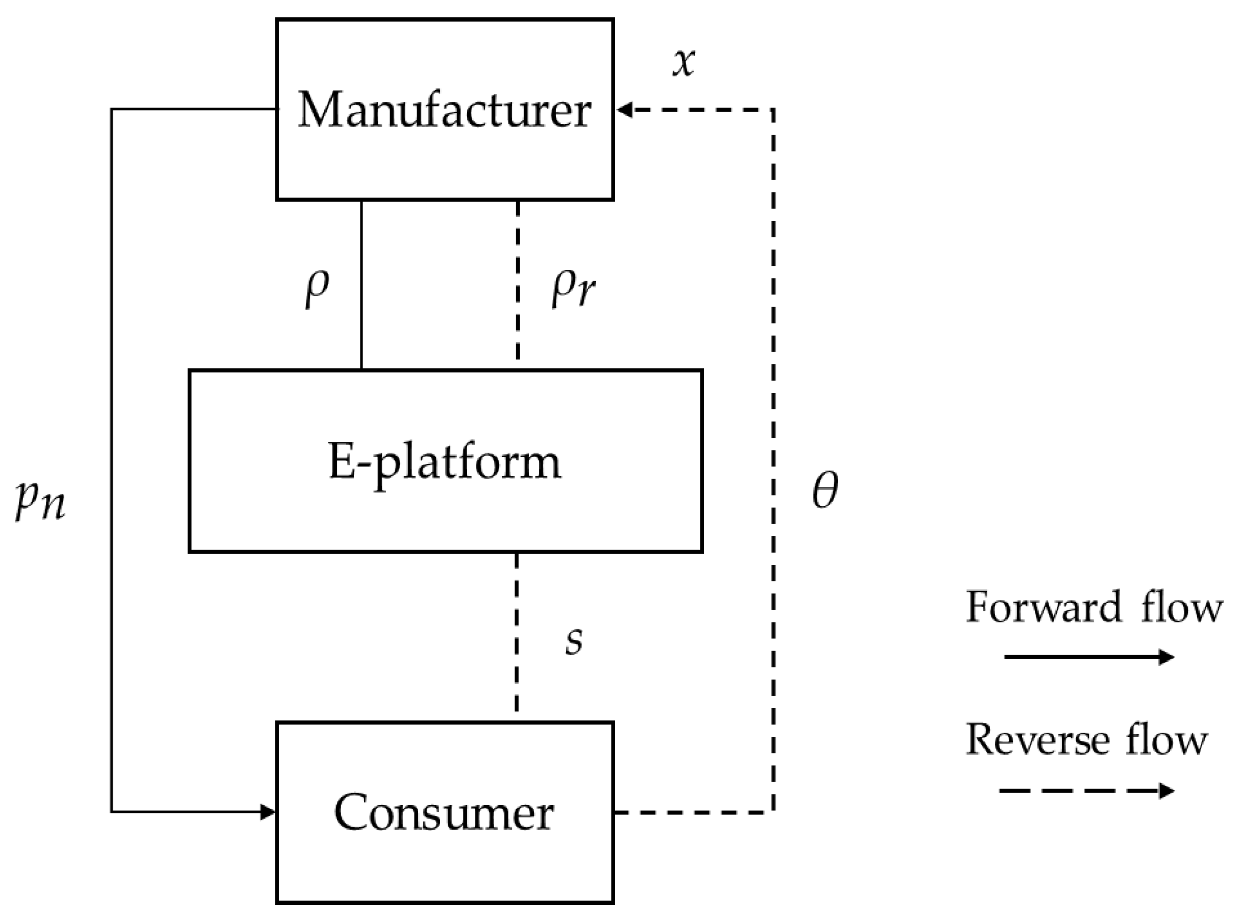
Figure 2.
The decision sequence.
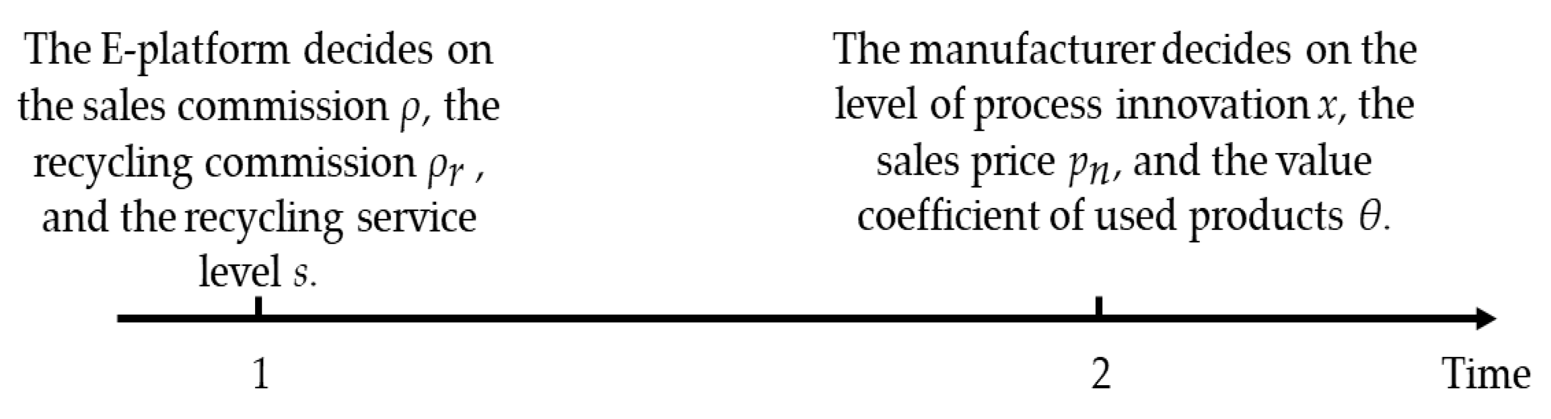
Figure 3.
The Schematic of FinTech platform financing.
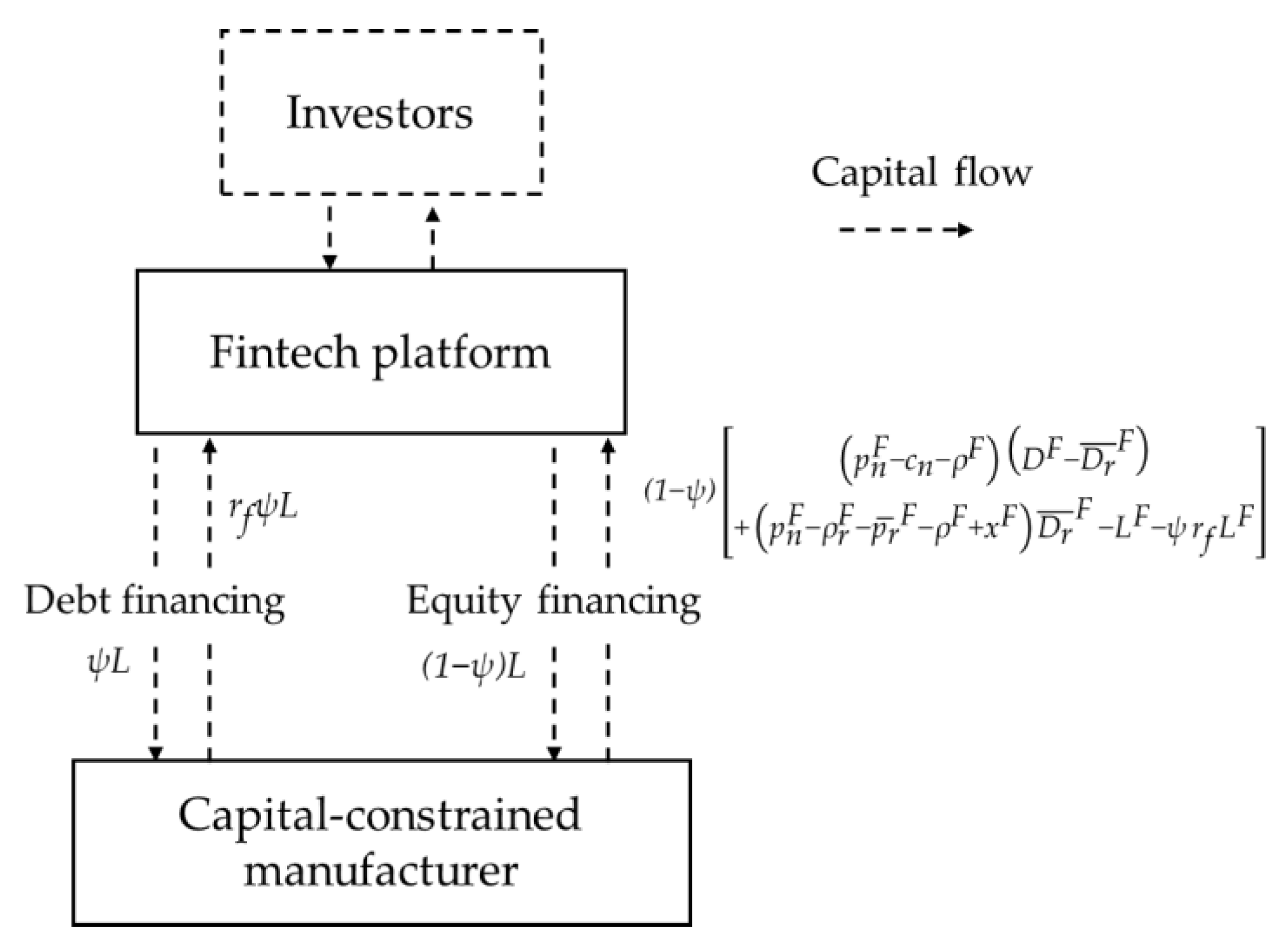
Figure 4.
Impact of and on ( and ).
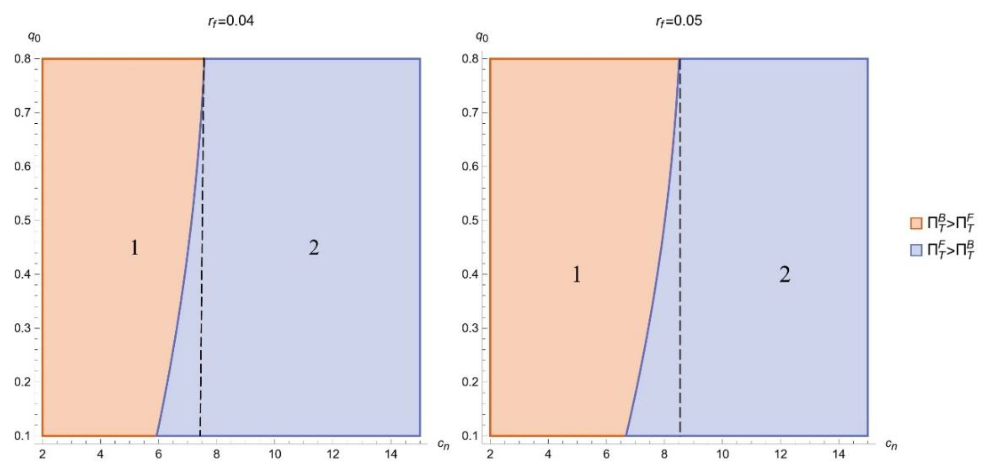
Figure 5.
Impact of and on
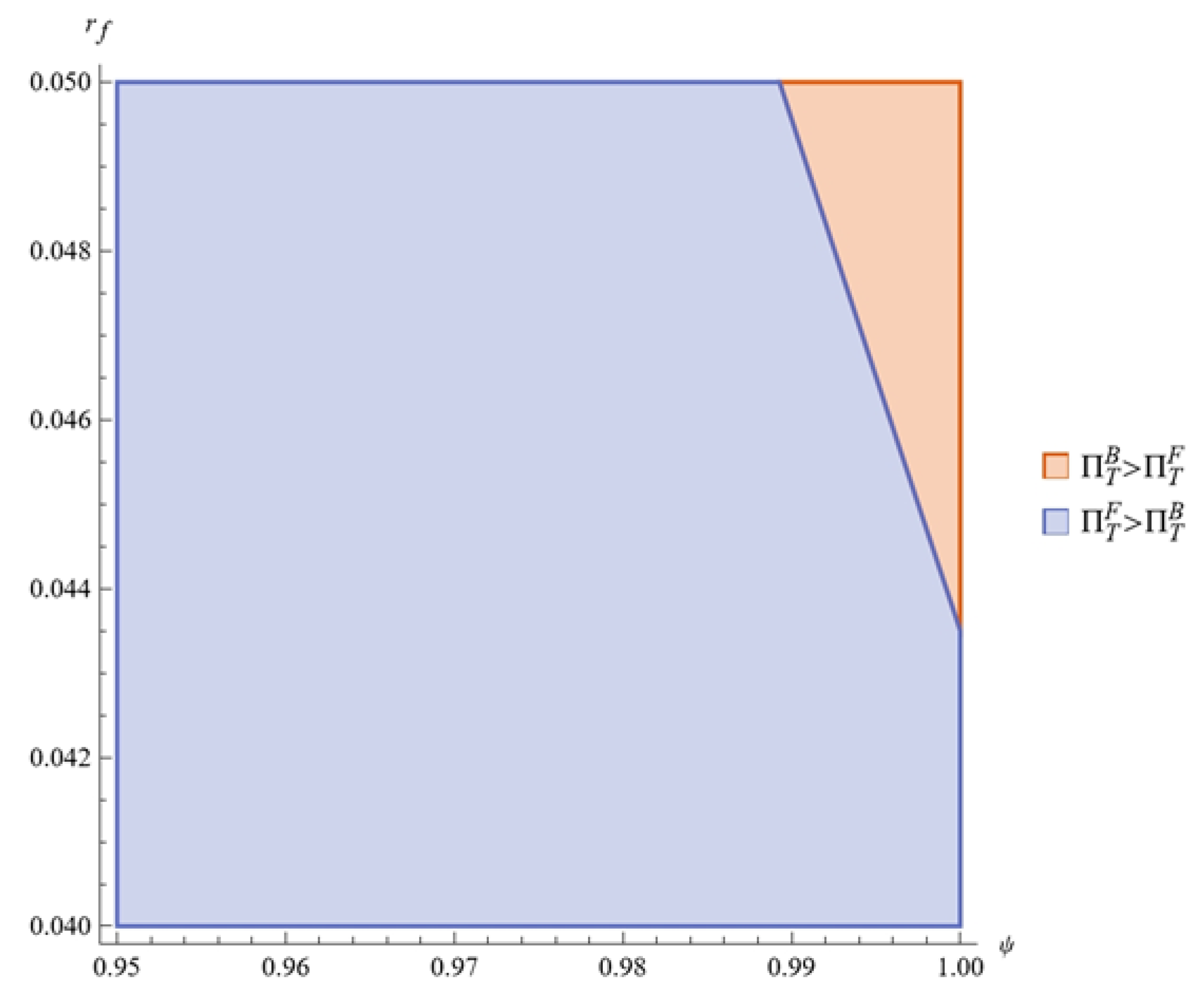

Table 1.
Comparison with related literature.
| Related literature | SC Structure | Sales Channel | Recycling Channel | Quality | Platform Service | PI | Capital Constraint | FC |
|---|---|---|---|---|---|---|---|---|
| Reimann, Xiong and Zhou [31] | CLSC | Offline | Offline | Fixed | √ | |||
| Yang, Tang and Zhang [33] | Forward | Offline | Offline | Fixed | √ | |||
| Wang, Yu, Shen and Jin [14] | CLSC | Online/Offline | Online/Offline | Fixed | √ | |||
| Reza-Gharehbagh, Arisian, Hafezalkotob and Makui [44] | CLSC | Offline | Offline | Fixed | √ | |||
| Cui, Zhou, Yu and Khan [20] | CLSC | Offline | Offline | Fixed | √ | |||
| Qin, Chen, Zhang and Ding [10] | CLSC | Offline | Offline | Uncertain | ||||
| Wang, Wang, Cheng, Zhou and Gao [6] | CLSC | Online | Online | Fixed | √ | √ | ||
| Chen, Tian, Chan, Tang and Che [41] | CLSC | Online | Online | Fixed | √ | |||
| Guo and Chen [29] Qian, Ignatius, Chai and Valiyaveettil [36] |
CLSC | Offline | Offline | Uncertain | ||||
| Barman [21] | Forward | Offline | Offline | Fixed | √ | |||
| Verma and Mishra [46] | CLSC | Offline | Offline | Fixed | √ | |||
| This study | √ | Online | Online | Uncertain | √ | √ | √ | √ |
Table 2.
Notations and their definitions.
| Notations | Definitions |
|---|---|
| Decision variables | |
| The sales commission. | |
| The recycling commission. | |
| The platform recycling service level. | |
| The PI level. | |
| The sales price of new products. | |
| The quality-based value coefficient of used products. | |
| Parameters | |
| The market size of the product. | |
| The sales price sensitivity coefficient. | |
| The recycling price sensitivity coefficient. | |
| The recycling service level sensitivity coefficient. | |
| The recycling price. | |
| The fixed payment. | |
| The quality level of the used product follows the uniform distribution of [0, 1]. | |
| The quality threshold for used products that can be remanufactured. | |
| The unit cost of manufacturing/remanufacturing. | |
| The PI cost coefficient. | |
| The manufacturer's loan size. | |
| / | The financing interest rate for the bank/FinTech platform, / |
| The DF ratio. | |
| The expected profit of the E-platform | |
| The expected profit of the manufacturer | |
| The expected overall profit of the ECLSC | |
| Indexes | |
| Superscript N, B, F | Model NC, BF, FPF |
Table 4.
Parameter settings.
| Parameter | Range | Other Parameters | ||||||||
| 30 | 1 | 15 | 0.5 | 0.95 | 0.0435 | 2 | 1 | 0.04/0.05 | ||
| Parameter | Range | Other Parameters | ||||||||
| 30 | 1 | 15 | 0.5 | 0.95 | 0.0435 | 2 | 1 | 0.04/0.05 | ||
| Parameter | Range | Other Parameters | ||||||||
| 30 | 1 | 15 | 0.5 | 0.95 | 0.0435 | 2 | 2 | 0.04/0.05 | ||
Disclaimer/Publisher’s Note: The statements, opinions and data contained in all publications are solely those of the individual author(s) and contributor(s) and not of MDPI and/or the editor(s). MDPI and/or the editor(s) disclaim responsibility for any injury to people or property resulting from any ideas, methods, instructions or products referred to in the content. |
© 2025 by the authors. Licensee MDPI, Basel, Switzerland. This article is an open access article distributed under the terms and conditions of the Creative Commons Attribution (CC BY) license (http://creativecommons.org/licenses/by/4.0/).
Copyright: This open access article is published under a Creative Commons CC BY 4.0 license, which permit the free download, distribution, and reuse, provided that the author and preprint are cited in any reuse.


