
Submitted:
12 November 2025
Posted:
13 November 2025
You are already at the latest version
Abstract
Analysis of a Crowdsourcing Markovian Queue with Phase-type Service is considered in this paper. In this model, a customer not only receives service but assists in delivery. In other words, in a retail environment, while some customers shop in-store, others place orders online or by phone and require home delivery. Store management can utilize online customers as couriers to complete these deliveries. However, because not every customer may agree to take part, a probabilistic element is included to capture the chances of their participation. The model also incorporates imperfect service, reflecting cases where deliveries may fail or require rework, and working breakdowns, representing partial disruptions in service capacity rather than complete stoppages. To analyse the system under steady-state conditions, matrix-analytic methods are applied. Numerical examples illustrate the significant benefits of incorporating these dynamics into traditional queueing models.
Keywords:
crowdsourcing
; working vacation policy
; imperfect service
MSC: 60K20; 60K25
1. Introduction
Crowdsourcing means a model where one customer receives service from another who is available to serve. Crowdsourcing has become popular in industries like food, hotels, and electronics. It has also been applied across diverse fields such as healthcare, computer science, environmental sciences, business, and marketing to improve efficiency and optimize resource allocation. For example, in healthcare, patients who have undergone treatment may share their experiences or provide support to new patients through peer mentoring programs. In computer science, crowdsourced platforms harness user contributions to improve artificial intelligence models or software development. Environmental sciences leverage crowdsourcing to collect and analyze data from volunteers, helping researchers monitor climate change or biodiversity.
The learning of queueing representations with working vacations has gained significant attention in recent years due to its practical applications in service systems, telecommunications, and manufacturing. Shrivastava and Rathore [1] investigated a Markovian queueing model with a single server, incorporating features such as distinct types of working vacations, vacation breaks, and customer abandonment. Their study offers meaningful perspectives on the system’s performance under these scenarios. Similarly, Rathore and Shrivastava [2] analyzed an M/M/1 queueing system incorporating an unreliable server with partial breakdowns during working vacations, demonstrating the impact of server failures on queue performance.
A queueing system with multiple working vacations and encouraged arrivals was explored by Prakati and Julia [3], using the M/M(a,b)/1 model to derive performance measures and demonstrate real-life applications. In a related study, Singh et al. [4] investigated a transient Markovian queueing model that offers options between regular and working vacations, providing a cost analysis and numerical evaluation of system performance. These studies collectively contribute to the understanding and optimization of queueing systems with working vacation policies, highlighting their importance in modern operational research.
Ayyappan and Arulmozhi [5] introduced a priority queueing model with delayed working vacations, considering multiple real-world factors such as immediate feedback and customer impatience. Ayyappan and Karpagam [6] explored a non-Markovian single-server queueing model characterized by batch arrivals, general bulk service, server failures and repairs, a single vacation policy, and the presence of a standby server. They obtained the probability generating function for the queue length at a random time and evaluated several performance metrics of the system. For modelling and analysing crowdsourcing Markovian queues, artificial intelligence (AI) techniques can be employed to enhance both efficiency and accuracy. A relevant example is provided by Zhang et al. [7], who propose a reinforcement learning-based edge server placement strategy for the intelligent Internet of Vehicles environment.
A retrial queueing system with group service and impatient customers was analyzed by D’Arienzo et al. [8], highlighting its applicability in telecommunication systems where bulk service and impatience are significant. Strategic behavior in an M/M/1 double orbit retrial queue with imperfect service and vacations was studied by Dhibar and Jain [9], providing insights into customer decision-making and system optimization under interruptions. Furthermore, Jain et al. [10] examined a Markovian working vacation queue incorporating imperfect service, balking, and retrial phenomena, providing insights into customer behavior under such conditions.
A non-Markovian queueing model with batch arrivals, phase-type service, and multi-vacation was examined by Radha et al. [11], with applications described in cloud computing. The following survey articles, queueing models with customer’s impatience by Anjali and Kolledath [12] and queueing models with discouragement policies and vacation by Sharma et al. [13] are remarkable. Haghighi et al. [14] investigated busy periods and queue length (steady-state and transient) of a single-server Poisson queue with delayed service, to set the tone for more complicated models. They analyzed their model by considering M/G/1 as well as the Erlang phase (stage) processes to set up differential difference equations for approximating a non-Markovian system.
The body of research on tandem queue analysis is extensive. Therefore, this discussion focuses exclusively on studies addressing dual tandem systems with multi-server stages and arrivals modeled by the Markov Arrival Process (MAP). Compared to the widely used stationary Poisson process—a special case of the MAP—the MAP provides a more realistic mathematical representation of bursty and correlated input processes observed in real-world systems. The MAP was originally introduced as a flexible and general framework for modeling arrival processes in [15].The model is investigated using the known results for Quasi-Birth-and-Death processes; see [16]. Chakravarthy et al. [17] used a single-server queueing framework with degradation, failures/breakdowns, and repairs, aiming to provide a realistic framework for analyzing and managing service systems under such conditions.
In [18] investigate a single-server queueing model with a Markovian arrival process (MAP) where served customers may act as temporary secondary servers. Their steady-state analysis using QBD and GI/M/1 formulations provides insights into performance measures and system dynamics. In [19] analyze a dual tandem queueing model for managing parcel pick-up networks, incorporating batch transfers, customer no-shows, and threshold-based order admissions. Their study offers insights into optimizing warehouse capacity and admission policies through steady-state performance evaluation.
2. Related Work
In Chakravarthy, [20,21] analyzed a multi-server queueing system with Poisson arrival patterns and exponential service durations, focusing on its application in crowdsourcing environments. Crowdsourcing has been applied in fields such as healthcare, computer science, and business. Recent studies have examined related queueing models like M/M/c, MAP/PH/1, and MAP/PH/c. This paper introduces vacation and working vacation concepts in a MAP/PH/1 queueing model for crowdsourcing as the baseline framework (see [20]). The proposed model extends it by incorporating imperfect service, probabilistic customer participation, and working breakdowns.
The model has broad practical applications in systems where human participation is uncertain and service reliability fluctuates. In healthcare crowdsourcing, volunteers or remote workers may contribute irregularly, introducing probabilistic participation and imperfect service outcomes. These examples demonstrate how the proposed model captures real-world variability in availability, performance, and service quality.
Shajin and Krishnamoorthy [22] propose a novel stochastic decomposition framework tailored to a combined retrial queue and inventory management model. They rigorously derive performance metrics by decoupling the queueing dynamics from inventory-level fluctuations, enabling analytical tractability. Their results illustrate how retrial behavior and restocking policy jointly affect system stability and cost, filling a gap between isolated queueing and inventory models. Shajin and Krishnamoorthy [23] extend classical queueing-inventory systems by incorporating MAP arrivals and PH-distributed service times. Their model introduces probabilistic customer behavior, item returns, and a feedback mechanism, enhancing realism. They develop new performance metrics and numerical methods to optimize revenue under a dynamic replenishment policy.
In this paper, we propose to investigate the operation of an order crowdsourcing, imperfect service, working vacation within a two-types customers. The system is a single-server queue handling two customer types: Type 1 visits the facility with limited waiting space, while Type 2 orders online with unlimited capacity. Both types arrive according to a Markovian arrival process. Service times follow phase-type distributions. During working vacations, the server serves Type 1 at a reduced rate, and service may need to be repeated if imperfect. Served Type 1 customers may assist Type 2 customers, implementing a crowdsourcing mechanism. The server is subject to breakdowns, providing slow service during failures, followed by repair. This model integrates working vacations, imperfect service, crowdsourcing, and breakdown-repair in a single framework.
2.1. Motivation
The motivation behind these models can be understood in the context of online retail and delivery services, particularly for products like books and articles. For example, consider an online bookstore such as Amazon or Flipkart. One group of customers visits physical outlets or pick-up points to purchase books, while another group orders online for home delivery. The store management can leverage in-store customers to assist in fulfilling online orders, such as by picking up books for delivery, reviewing or recommending articles, or sharing their experiences online. Since not all in-store customers may be willing or able to perform these tasks, a probability factor represents the likelihood of a customer acting as a “crowdsourced server.” Similarly, marketing campaigns like referral programs or “bring a friend” initiatives incentivize existing customers to help promote books or online articles, effectively expanding the customer base. This approach helps businesses reduce delivery and marketing costs, enhance customer engagement, and create a collaborative ecosystem between different types of customers.
2.2. Research Gap
Based on existing studies, concepts such as crowdsourcing, imperfect service, and server breakdown with repair have mostly been explored individually within traditional queueing systems, often through mechanisms like working vacations and service disruptions. To the best of our knowledge, no prior research has simultaneously considered crowdsourcing, imperfect service, and breakdown-repair in a unified Markovian arrival process in queueing model. We develop a queueing system that incorporates Markovian arrival process for Type 2 customers, phase-type service, crowdsourcing and imperfect service, and examine how the server can enhance the system’s profitability through sensitivity analysis.
2.3. Contribution of the Model
The following presumptions are to be carried out in this paper:
- This model investigates the crowdsourcing, imperfect service, and server breakdown with repair.
- This model uses the matrix analytic method to determine the proposed system’s steady-state probability vector.
- The numerical illustration analyzed the system performance measures using parameter variation.
3. Model Development
This model considers a single-server queueing system with a crowdsourcing Markovian queue with phase-type and imperfect service, working vacations, breakdown and repair. It has an infinite and a finite waiting hall attached to the server.
3.1. Working Vacations
After completing customer service, the server may take a vacation when the queue is empty. If customers arrive during this vacation period, the server provides service at a reduced rate compared to the normal service rate.
3.2. Crowdsourcing
In computer networks, usually a server provides services (like hosting a website) and a client/customer uses it. But sometimes, a customer (client machine) can act as a server too. It is known as Crowdsourcing. For example, in file sharing (like BitTorrent), your computer (as a customer) downloads files from others, but at the sametime, it also uploads and shares pieces of the file to other users. So your computer is both a client (receiving data) and a server (sending data to others).
3.3. Imperfect Service
When the server’s performance is imperfect, customers may request additional service if the initial service is unsatisfactory. If a new customer arrives while the server is busy, the customer may either leave the system or seek immediate re-service.
3.4. Breakdown and Repair
Server breakdowns are a critical factor to consider in practical service systems and manufacturing industries. During service delivery, the server may experience a failure that requires immediate repair. Throughout the repair process, the server suspends customer service, resuming operations only after the repair is completed to continue serving the interrupted customers.
- We examine a queueing system with a single server that handles two distinct categories of customers. Type 1 customers, denoted as , arrive according to a Markovian Arrival Process (MAP) characterized by the matrix pair of order . Here, governs transitions without customers arrivals, while corresponds to transitions involving a customers arrival. The arrival rate of customers is denoted by . Similarly, Type 2 customers, denoted as , follow a MAP represented by of order , where captures transitions without arrivals and captures transitions with a arrival. The arrival rate of customers is denoted by .
- If a customers arrives and encounters the server idle on working vacation, they begin service immediately, albeit at a reduced service rate. If the server is occupied, the customer enters the queue and will be served in the order of arrival (first-come-first-served) when the server becomes free. A customers is turned away if the system has reached its capacity upon arrival, based on the assumption that the waiting area for customers is limited to N spots. customers physically visit the facility (e.g., a store) to receive service, whereas customers place orders remotely (e.g., via phone or online). This distinction justifies the limited waiting area for customers and the unlimited waiting space for consumers, with no restrictions on the number of units in the system (i.e., they have an infinite buffer). If a customers notices that the server is not busy, they will remain in the system until the server is ready to serve them.
- The service durations for both customer types are modeled using phase-type distributions, represented by and of orders and , respectively. After a service is completed and no customers remain in the system, the server begins a vacation. The duration of this vacation is modeled by an exponential distribution with rate . A vacation is terminated prematurely if an customers arrival occurs during this period. During a vacation, the server offers service to arriving customers but at a reduced service rate. It is important to note that only customers can be served during vacation mode.
-
During a vacation, the service times for customers are modeled by a phase-type distribution, represented by of order , where . The server operates at this reduced service rate throughout the remaining vacation period. After the vacation ends, the server re-enters the system. If any customers are waiting, the server immediately switches to the normal service rate and continues serving until the system becomes empty. If no customers are present, the server remains idle.Let and denote the regular service rates for and customers, respectively:and the service rate during a working vacation is . After being served during a working vacation, a customer may not be satisfied with the service quality. In such cases, the server repeats the same service (re-service) with probability . If the customer is satisfied, they depart the system with probability , where .
-
While customers are being served by the server, customers may be served either by the system server or by a customers who has already completed their own service and is available to act as a temporary server. A customers can be served by a customers under the following conditions:
- -
- The customers must have just completed their service and must choose to assist in serving a customers.
- -
- There must be at least one customers waiting for service at the moment the customer becomes available. In other words, the customers must not have already commenced service with the system server.
- -
- After completing service for a customers, the customers can instantaneously provide service to a customers. However, at any given time, a customers can serve only one customers.
- With probability , we suppose that a served customers will be available to service a customers under the previously mentioned conditions, where . With a probability of , the consumers who was served will exit the system. The system server provides service to a customers when a service is finished. The server will serve a customers if one is in the system, but only if no customers are waiting. Customers with are presumed to have non-preemptive precedence over those with . For analytical purposes, if a customers chooses to serve a customers, that client is instantly eliminated from the system. This assumption simplifies the analysis by eliminating the need to track customers once they are assigned to a customers for service.
- When a breakdown occurs during a regular service period, we assume that breakdowns are generated according to an exponential distribution with rate . During a breakdown, the server continues delivering service to the current customer, but at a reduced service rate. After completing the ongoing slow service, the server undergoes a repair period. During the working breakdown period, the server provides slow service to customers, where the service times follow phase-type distributions represented by for customers, with and of order , and for customers, with and of order . The corresponding slow service rates are given by , . The repair times follow a phase-type distribution with representation of order l, and the repair rate is . A diagram of the model is shown in Figure 1.
4. Matrix Form of the QBD Generator
4.1. Assumptions
We will use the following assumptions throughout the model:
- =.
- =.
- : Total Type-2 customers in the system at epoch t.
- : Total Type-1 customers in the system at epoch t.
- represents the server’s status at epoch t.
- denotes the phase of the repair process at time t.
- represents the service phase for a customer at time t.
- represents the service phase for a customer at time t.
- refers to the phase of the arrival process at time t.
- refers to the phase of the arrival process at time t.
Let , where
Y=, is a with state space
where
and for
4.2. The Infinitesimal Generator Matrix
Suppose that the generator of the CTMC is of the quasi-birth-and-death (QBD) type in the matrix, , such that the generator is of the form gives by:
where the square matrices and are such that:
The following describes Markov chain transitions and the corresponding rates:
- contains transitions within level 0.
- Since Q is a generator, its diagonal elements are negative. The modules of these entries are the intensity of Markov chain leaving its states.
- When a Type 1 customer arrives on the system and the server starts the service. The corresponding intensities are the diagonal elements of the matrix .
- Vacation completion for the server. The corresponding intensities are the diagonal elements of the matrix .
- A server finishes slow service for customers with probability . The corresponding intensities are the diagonal elements of the matrix .
- A server is interrupted due to breakdown. The intensities of this event are defined by the matrix . The matrix governs,
, , ,
,
,
, ,
- contains transitions within level 0 to 1.
- When a Type 2 customer arrives on the system with finite capacity N. The corresponding intensities are the diagonal elements of the matrix .The matrix governs
,
- contains transitions within level 1 to 0.
- A server finishes slow service for customers with probability and after service completion will start the fresh service for waiting customers. The corresponding intensities are the diagonal elements of the matrix .
- A server completes the service for customers. The rates of this event occurrence are defined by the matrix . The matrix governs,
- contains transitions within level n for .
- Its diagonal elements are negative. The modules of these entries are the intensity of Markov chain leaving its states.
- When a Type 1 customer arrives on the system and the server starts the service. The corresponding intensities are the diagonal elements of the matrix .
- After vacation completion, the server start the service for Type 2 customers. The corresponding intensities are the diagonal elements of the matrix .
- A server finishes slow service for customers with probability . The corresponding intensities are the diagonal elements of the matrix .
- A server is interrupted due to breakdown. The intensities of this event are defined by the matrix . The matrix governs,
,
, ,
,
, ,
, ,
,
,
, ,
, ,
, , ,
,
,
, ,
, ,
, ,
, ,
, ,
, ,
,
, ,
- contains transitions represents transitions from n to for . When a Type 2 customer arrives on the system with finite capacity N. The corresponding intensities are the diagonal elements of the matrix .
- The matrix governs,
,
, , ,
, , ,
, ,
- contains transitions represents transitions from n to for .
- A server finishes slow service for customers with probability and after service completion will start the fresh service for waiting customers. The corresponding intensities are the diagonal elements of the matrix .
- A server completes the service for customers and after service completion will start the fresh service for waiting customers. The rates of this event occurrence are defined by the matrix . The matrix governs,
,
, ,
, ,
, ,
, ,
, .
The matrices R is given by where the sequence of matrices is defined as:
For stable systems, the sequence is monotonically increasing and converges to R. Hence, R can be evaluated by successive substitutions using equation 4, until a desired level of convergence is achieved.
5. Analysis
5.1. Condition for Stability
Let be an irreducible infinitesimal generator matrix with order
.
where
, , , , , , , , , , , , , , , , , , , , , , .
Let denote the steady-state probability vector of the matrix F, satisfying the conditions and . The vector is partitioned as follows:
where the dimensions of each component are given by:
- has size ,
- , , and each have size ,
- has size ,
- has size ,
- has size ,
- has size .
The steady-state probability vector is obtained by solving the following system of equations:
subject to normalizing condition
The LIQBD description of the model indicates that the queueing system is stable if and only if the left drift exceeds the right drift (see Theorem 3.1.1 of Neuts [16]), that is,
Multiplying by in Equation 6 and substituting Equations 6 and 7 into Equation 5, we obtain
5.2. The Stationary Probability Vector
Let Z be the solution for the infinitesimal generator Q of the process {Z(t): }. This Z is splitted up depending on status of the server where is of size and are of size . As Z is a vector satisfies the condition
The probability vector Z follows a matrix geometric structure under the steady state is
where R is the quadratic equation’s lowest non-negative solution
and the vector are obtained with the help of succeeding equations:
subject to a condition normalization
As an outcome, we can employ the structure of something like the coefficient matrices to compute the vector Z and the matrix R using the Logarithmic Reduction Algorithm in Latouche and Ramaswami [24].
6. Busy Period Analysis
- A busy period is commonly described as the interval of time between when customers join an empty system with positive inventory and when they exit the system empty after obtaining their services in a queueing inventory system of single-server demonstration. Consequently, this marks the beginning of the shift from level 1 to level 0. The first return time of level zero, followed by at least one visit to any subsequent level, is an analogy for the busy cycle.
- A notable concept introduced by Latouche and Ramaswami [25] is the fundamental period, which pertains to the time taken to transition from level i to , where within the framework of a QBD.
- A notable feature of this approach is that for each level i, , there are states associated with it. This quantitative representation captures the complexity and variability present within the system across different levels.
- The QBD stream conditional probability originates in the state at time and goes to the level but not earlier time x, allowing for changes. The variable represents the u transition to the left and reaching the state .
The transition matrix
and the matrix is shown as , satisfying
Let , is an initial passage time without the boundary states.
Otherwise, the G matrix’s values could be calculated using the concept of a logarithmic reduction procedure [24].
For boundary levels 1 and 0, we get the equations provided by,
Due to the stochastic character of and the matrices are utilised to calculate the subsequent cases. The following are the instants that can be calculated at and .
7. Evaluating System Operations
In this section, we calculate some system performance measures useful in qualitative interpretation of the model under study. We shall use the following representations:
7.1. Estimated Number of Customers Currently in the System
7.2. Probability of the Server Being Inactive During a Working Vacation Period
Let denotes the invariant probability of the number of customers in the queue is i for , the number of customers in the system is d for , the server is inactive in working vacation is 0, and the number of arrival phases is for and , for .
7.3. Probability of the Server Being Active During a Working Vacation Period
Let denotes the invariant probability of the number of customers in the queue is 0, the number of customers in the system is d for , the server is active in working vacation is 1, the number of customers service phase is for and the number of arrival phases is for and , for .
7.4. Probability That the Server Is Reservice in Working Vacation
7.5. Probability of the Server Being Inactive During a Normal Operation
Let denotes the invariant probability of the number of customers in the queue is 0, the number of customers in the system is d for , the server is idle in normal period is 3, and the number of arrival phases is for and , for .
7.6. Probability of the Server Handling Customers in Normal Mode
7.7. Probability That the Server Is Active () in Normal Mode
7.8. Probability That the Server Is Busy
7.9. Probability That the Server Is Idle
7.10. Particular Case
When parameters representing imperfect service, working breakdowns, and probabilistic participation are deactivated (i.e., set to ideal or null values), the model simplifies to the Chakravarthy [20] framework without those additional complexities. This reduction confirms structural validity—showing that the extended model is a true generalization rather than an unrelated formulation.
Furthermore, the analytical results—such as steady-state probabilities, mean queue length, and system utilization—were cross-checked to ensure they converge to the same values as those derived from the baseline model when the extension parameters are neutralized. Such consistency provides mathematical assurance that the new features have been integrated correctly into the queueing framework.
8. Numerical Implementation
To generate numerical results, we utilized various MAP representations for incoming arrivals, ensuring that their mean values are equal to 1, following the approach suggested by Chakravarthy [26].
- customers with Erlang arrival distribution- :
- customers with Erlang arrival distribution - :
- Exponential arrival pattern -:
- Exponential arrival pattern-:
- Hyper exponential arrival-:
- Hyper exponential arrival-:
For the servicing and repair progression, take into account the following PH-distributions:
- Erlang service :
- Erlang repair :
- Exponential service :
- Exponential repair :
- Hyper exponential service :
- Hyper exponential repair :
Illustrative 1. We investigated the implications of the the service rate on the determined system size (. We define , , , and , , , , , , , , such that the system remains stable.
- The matrix R using the Logarithmic Reduction Algorithm in Latouche and Ramaswami [24]. Numerical results were computed iteratively up to for Erlang distribution, for exponential distribution and for hyperexponential distribution. At this level, the solution demonstrated convergence with an accuracy of up to six significant digits. The computations were performed using MATLAB software (R2019b), ensuring precise numerical implementation and consistency. This confirms the stability and reliability of the obtained results.
- As the service rate increases, the system processes customers or orders more efficiently, thereby reducing congestion and queue lengths. The service rate represents the average number of customers or jobs a server can handle per unit of time. It directly governs how quickly the system can process incoming tasks and therefore plays a crucial role in determining system congestion and stability.
- In relation to all other arrival times, the drops down quickly for and slowly for . Similarly, in terms of service times, the drops rapidly in and more slowly with . This suggests that systems exposed to variable (heterogeneous) arrival processes benefit more significantly from an increase in service rate, as higher compensates for irregular inflow patterns.

Table 1.
vs. service rate -.
| ERA | EXA | HEXA | |
| 11 | 0.273323 | 0.272934 | 0.327740 |
| 12 | 0.265213 | 0.267634 | 0.320544 |
| 13 | 0.258952 | 0.263574 | 0.315105 |
| 14 | 0.254005 | 0.260387 | 0.310875 |
| 15 | 0.250021 | 0.257834 | 0.307507 |
| 16 | 0.246757 | 0.255752 | 0.304772 |
| 17 | 0.244045 | 0.254029 | 0.302514 |
| 18 | 0.241763 | 0.252584 | 0.300622 |
| 19 | 0.239822 | 0.251360 | 0.299017 |
| 20 | 0.238153 | 0.250310 | 0.297641 |
Table 2.
vs. service rate -.
| ERA | EXA | HEXA | |
| 11 | 0.264056 | 0.289999 | 0.344393 |
| 12 | 0.257478 | 0.282631 | 0.334970 |
| 13 | 0.252446 | 0.277002 | 0.327868 |
| 14 | 0.248502 | 0.272595 | 0.322372 |
| 15 | 0.245343 | 0.269071 | 0.318024 |
| 17 | 0.240639 | 0.263832 | 0.311646 |
| 18 | 0.238852 | 0.261847 | 0.309260 |
| 19 | 0.237336 | 0.260165 | 0.307251 |
| 20 | 0.236037 | 0.258726 | 0.305543 |
Table 3.
vs. service rate -.
| ERA | EXA | HEXA | |
| 11 | 0.541994 | 0.416627 | 0.366188 |
| 12 | 0.507018 | 0.392839 | 0.353202 |
| 13 | 0.479533 | 0.374753 | 0.344100 |
| 14 | 0.457402 | 0.360665 | 0.337594 |
| 15 | 0.439211 | 0.349462 | 0.332868 |
| 16 | 0.423996 | 0.340394 | 0.329391 |
| 17 | 0.411079 | 0.332939 | 0.326806 |
| 18 | 0.399972 | 0.326728 | 0.324870 |
| 19 | 0.390314 | 0.321490 | 0.323411 |
| 20 | 0.381834 | 0.317027 | 0.322309 |
Illustrative 2. We analyzed the effect of the server’s service rate, denoted as , influences the probability that the server is busy during normal mode, represented by in Table 4, Table 5 and Table 6. To ensure system stability during this analysis, the following parameters were defined: , , , , , , , , , and .
- The matrix R using the Logarithmic Reduction Algorithm in Latouche and Ramaswami [24]. Numerical results were computed iteratively up to for Erlang distribution, for exponential distribution and for hyperexponential distribution. At this level, the solution demonstrated convergence with an accuracy of up to six significant digits. The computations were performed using MATLAB software (R2019b), ensuring precise numerical implementation and consistency. This confirms the stability and reliability of the obtained results.
- As the Type-1 service rate increases, the system’s ability to handle incoming tasks improves, allowing the server to process requests more quickly. Consequently, the proportion of time that the server remains busy during normal operation, denoted as , decreases. A higher service rate thus alleviates congestion and reduces queue lengths, as tasks are completed faster than they arrive, leading to fewer intervals in which the server is continuously occupied.
- When comparing different arrival distributions, the rate at which decreases varies depending on the variability of arrivals. Under hyper-exponential arrivals, which exhibit high variability and burstiness, an increase in produces a more pronounced reduction in , since the system benefits substantially from faster service during sudden demand spikes. In contrast, for Erlang arrivals, where inter-arrival times are more regular, the decline in is more gradual because the arrival process is smoother and less sensitive to service rate adjustments.
- Similarly, for different service-time distributions, the responsiveness of to changes in depends on service variability. When service times follow an Erlang distribution, which is more uniform, increasing rapidly reduces , as predictable and shorter service durations allow the server to become idle more frequently. However, under a hyper-exponential service pattern, characterized by higher variability, the reduction in is slower, since occasional long service times can still keep the server occupied even at higher service rates.
Illustrative 3.
- We fix the parameters as , , , , , , , , , , and to ensure that the system remains within the stability region, where the total service capacity exceeds the effective arrival rate.
- This behavior can be interpreted as follows: as the Type 2 service rate increases, the server completes tasks more rapidly, leading to shorter busy periods and more frequent idle intervals. In essence, a higher enhances the system’s processing efficiency, reducing congestion and waiting times. However, when the service rate grows significantly beyond the arrival rate, the server experiences extended idle times, reflecting potential over-provisioning of service capacity.
When the arrival rate, breakdown rate, and probability of dissatisfaction increase, the average queue size tends to grow because the system experiences higher input and reduced efficiency. A higher arrival rate means more customers enter the system per unit of time, while an increased breakdown rate decreases the effective service capacity as servers become unavailable more often. Likewise, a higher probability of dissatisfaction can lead to more re-service requests or inefficiencies, effectively increasing the workload. Together, these factors cause congestion, leading to longer queues. Conversely, when the service rate, repair rate, and probability of satisfaction increase, the average queue size decreases because the system processes customers more efficiently. A higher service rate allows faster completion of tasks, an improved repair rate reduces downtime, and a higher satisfaction probability lowers the likelihood of repeated service or complaints. As a result, the system clears customers more smoothly, leading to shorter queues and better overall performance.
9. Conclusion
This paper investigates a queueing model applicable to scenarios like crowdsourced operations, working vacations, service imperfections, functional breakdowns, and phase-type repair mechanisms. The framework permits the server to continue attending to a specific group of customers during vacation periods, though at a diminished service efficiency. By adopting a versatile class of arrival processes and representing service durations through phase-type distributions, we highlight the benefits of integrating these elements into traditional queueing theory. These advantages are further illustrated with comprehensive numerical simulations.
Author Contributions
All authors have made equal contributions to the conception, design, and writing of this manuscript.
Institutional Review Board Statement
Not applicable.
Informed Consent Statement
Not applicable.
Data Availability Statement
Not applicable.
Acknowledgments
The authors are very grateful to the reviewers for their valuable comments and suggestions, which improved the quality and the presentation of the paper.
Conflicts of Interest
The authors declare no conflict of interest.
Notations
The following notations are used in this manuscript:
| ⊗ | Kronecker product, producing a block matrix from two matrices of appropriate sizes. |
| ⊕ | Kronecker sum, generates a block matrix by combining two matrices of compatible sizes. |
| Refers to the identity matrix of size . | |
| e | A column vector of appropriate length, with all entries equal to one. |
| Markovian Arrival Process. | |
| Phase type distributions. |
Appendix A
Illustrative 4.
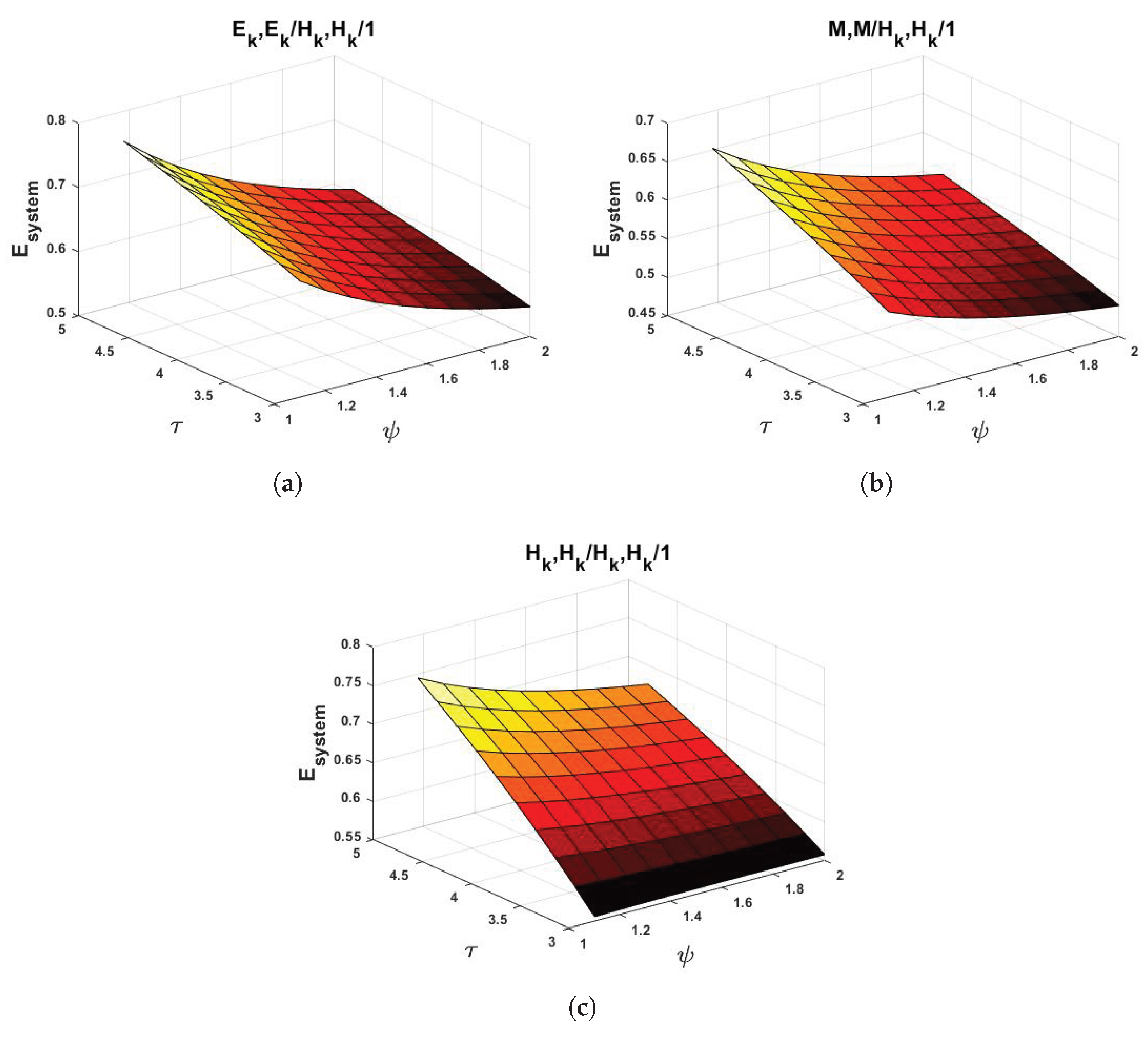
- When examining the influence of service-time distributions, increases sharply under the Erlang service (ERS) scenario, where the regularity of service times amplifies the impact of repeated breakdowns—each interruption extends queue lengths more significantly. In contrast, under the Exponential service (EXS) case, the increase in is more moderate, as the stochastic nature of service times allows for some inherent flexibility in handling interruptions.
- Similarly, considering arrival-time distributions, grows slowly under Erlang arrivals (ERA) due to their low variability and predictable inflow, which helps the system absorb disturbances more effectively. However, under Hyper-exponential arrivals (HEXA), where inter-arrival times are highly variable and bursty, increases rapidly. In such cases, bursts of arrivals coinciding with breakdowns intensify congestion and elevate system size significantly.
Figure A1.
vs. breakdown and repair rates.
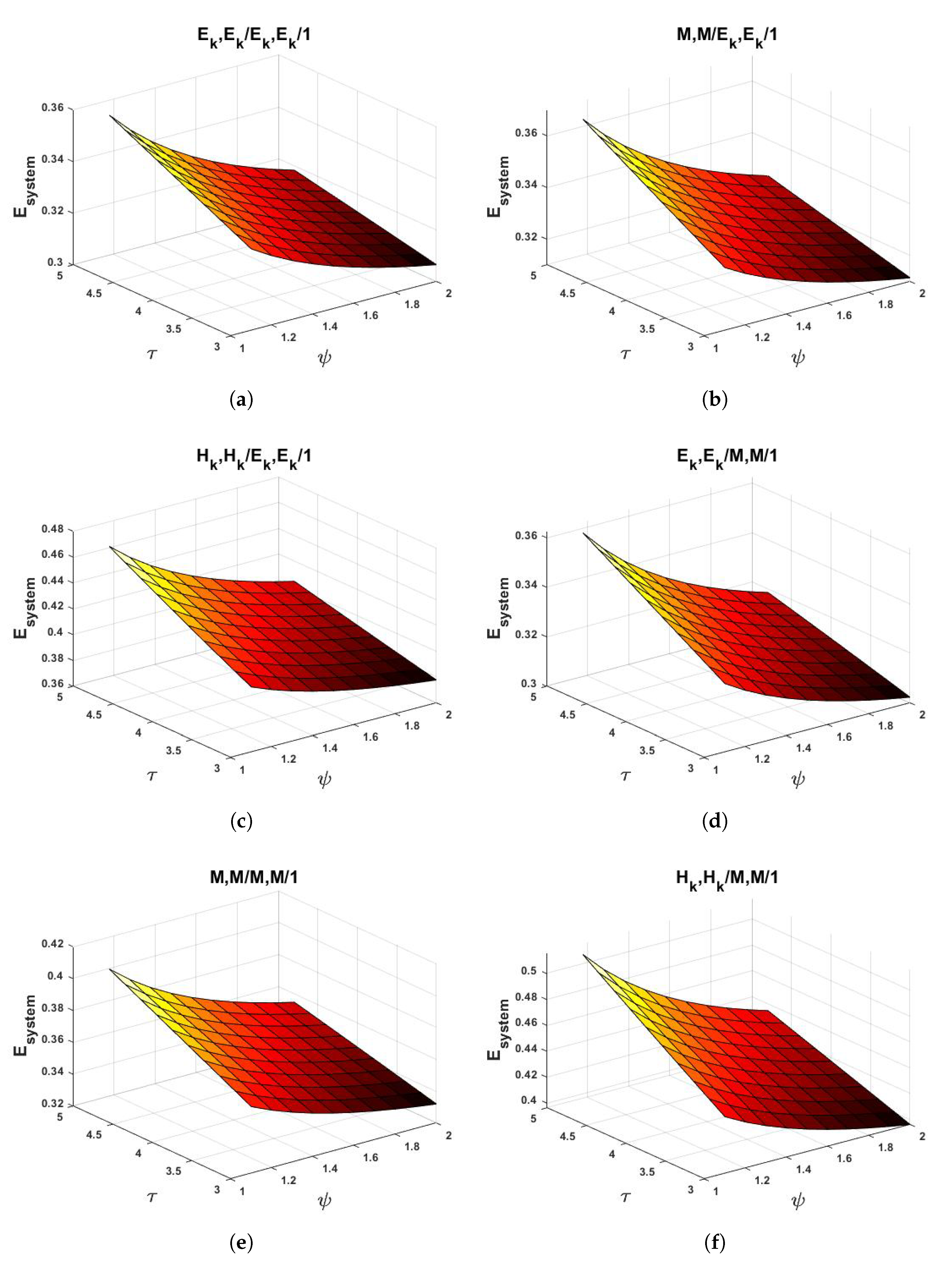
Figure A2.
vs. breakdown and repair rates.
References
- Shrivastava, R. K.; Rathore, R. Analysis of Single Server Markovian Queueing Model with Differentiated Working Vacation, Vacation Interruption, Soft Failure, Reneging of Customers. Int. J. Global Acad. Sci. Res. 2024, 5, 78–92. [Google Scholar] [CrossRef]
- Rathore, R.; Shrivastava, R. K. Analysis of M/M/1 Queueing Model with Removable and Unreliable Server, Partial Breakdown during Working Vacation, Setup with Repair. J. Math. Probl. Equ. Stat. 2024, 5, 141–155. [Google Scholar] [CrossRef]
- Prakati, P.; Julia, R. M. K. Analysis of Multiple Working Vacations Queuing System with Encouraged Arrival Using M/M(a,b)/1 Model. Baghdad Sci. J. 2024, 6, 9162–9175. [Google Scholar]
- Singh, M.; Jain, M.; Azhagappan, A. Cost Analysis of a Transient Markovian Queueing Model with Provision of Options between Regular and Working Vacation. Int. J. Math. Oper. Res. 2024, 10, 138906–138920. [Google Scholar] [CrossRef]
- Ayyappan, G.; Arulmozhi, N. Analysis of M, MAP/PH1, PH2/1 Non-preemptive Priority Queueing Model with Delayed Working Vacations, Immediate Feedback, Impatient Customers, Differentiate Breakdown, and Phase-Type Repair. Reliab. Theory Appl. 2023, 18, 64–79. [Google Scholar]
- Ayyappan, G.; Karpagam, S. An M[X]/G(a,b)/1 queueing system with server breakdown and repair, stand-by server, and single vacation. Int. J. Math. Oper. Res. 2019, 14, 221–235. [Google Scholar] [CrossRef]
- Zhang, Y.; Li, X.; Chen, H.; Wang, J. Reinforcement Learning-Based Edge Server Placement in the Intelligent Internet of Vehicles Environment. IEEE Trans. Intell. Transp. Syst. 2025. [Google Scholar]
- D’Arienzo, M. P.; Dudin, A. N.; Dudin, S. A.; Manzo, R. Analysis of a retrial queue with group service of impatient customers. J. Ambient Intell. Humaniz. Comput. 2020, 11, 2591–2599. [Google Scholar] [CrossRef]
- Dhibar, S.; Jain, M. Strategic Behavior for M/M/1 Double Orbit Retrial Queue with Imperfect Service and Vacation. Int. J. Math. Oper. Res. 2023, 15, 245–260. [Google Scholar]
- Jain, M.; Dhibar, S.; Sanga, S. S. Markovian Working Vacation Queue with Imperfect Service, Balking, and Retrial. J. Ambient Intell. Humaniz. Comput. 2022, 13, 1–20. [Google Scholar] [CrossRef]
- Radha, S.; Maragathasundari, S.; Swedheetha, C. Analysis on a non-Markovian batch arrival queuing model with phases of service and multi vacations in cloud computing services. Int. J. Math. Oper. Res. 2023, 24, 425–449. [Google Scholar] [CrossRef]
- Anjali, C. K.; Kolledath, S. Survey on queuing models with discouragement, policies, and vacation. Int. J. Math. Oper. Res. 2024, 28, 105–145. [Google Scholar] [CrossRef]
- Sharma, S.; Kumar, R.; Soodan, B. S.; Singh, P. Queuing models with customers’ impatience: a survey. Int. J. Math. Oper. Res. 2023, 26, 523–547. [Google Scholar] [CrossRef]
- Haghighi, A. M.; Mishev, D. P. A time-dependent tandem BMAP with balking and batch service with possible breakdown and delayed service. Queueing Models and Service Management 2025, 8(2), 35–63. [Google Scholar]
- Neuts, M. F. A versatile Markovian point process. Journal of Applied Probability 1979, 14, 764–779. [Google Scholar] [CrossRef]
- Neuts, M. F. Matrix-Geometric Solutions in Stochastic Models: An Algorithmic Approach; Courier Corporation: Chelmsford, MA, USA, 1994. [Google Scholar]
- Choudhary, A.; Chakravarthy, S. R.; Sharma, D. C. Impact of the degradation in service rate in MAP/PH/1 queueing system with phase type vacations, breakdowns, and repairs. Annals Operation Research 2023, 331, 1207–1248. [Google Scholar] [CrossRef]
- Chakravarthy, S.R.; Dudin, A.N.; Dudin, S.A.; Dudina, O.S. Queueing system with potential for recruiting secondary servers. Mathematics 2023, 11(3), 624. [Google Scholar] [CrossRef]
- Dudin, A.N.; Dudina, O.S.; Dudin, S.A.; Melikov, A. A dual tandem queue as a model of a pick-up point with batch receipt and issue of parcels. Mathematics 2025, 13(3). [Google Scholar] [CrossRef]
- Chakravarthy, S. R.; Ozkar, S. MAP/PH/1 queueing model with working vacation and crowdsourcing. Math. Applicanda 2016, 44. [Google Scholar] [CrossRef]
- Chakravarthy, S. R.; Dudin, A. N. A queueing model for crowdsourcing. J. Oper. Res. Soc. 2017, 68, 221–236. [Google Scholar] [CrossRef]
- Shajin, D.; Krishnamoorthy, A. Stochastic decomposition in retrial queueing-inventory system. RAIRO Oper. Res. 2020, 54, 81–99. [Google Scholar] [CrossRef]
- Shajin, D.; Melikov, A. Queueing inventory system with return of purchased items and customer feedback. RAIRO Oper. Res. 2025, 59, 1443–1473. [Google Scholar] [CrossRef]
- Latouche, G.; Ramaswami, V. A Logarithmic Reduction Algorithm for Quasi-Birth-Death Processes. J. Appl. Probab. 1993, 30, 650–674. [Google Scholar] [CrossRef]
- Latouche, G.; Ramaswami, V. Introduction to Matrix Analytic Methods in Stochastic Modeling; SIAM: Philadelphia, PA, 1999. [Google Scholar]
- Chakravarthy, S. R. Introduction to Matrix-Analytic Methods in Queues 1: Analytical and Simulation Approach—Basics; ISTE Ltd.: London, UK; John Wiley & Sons: New York, NY, USA, 2022. [Google Scholar]
Figure 1.
Schematic representation.
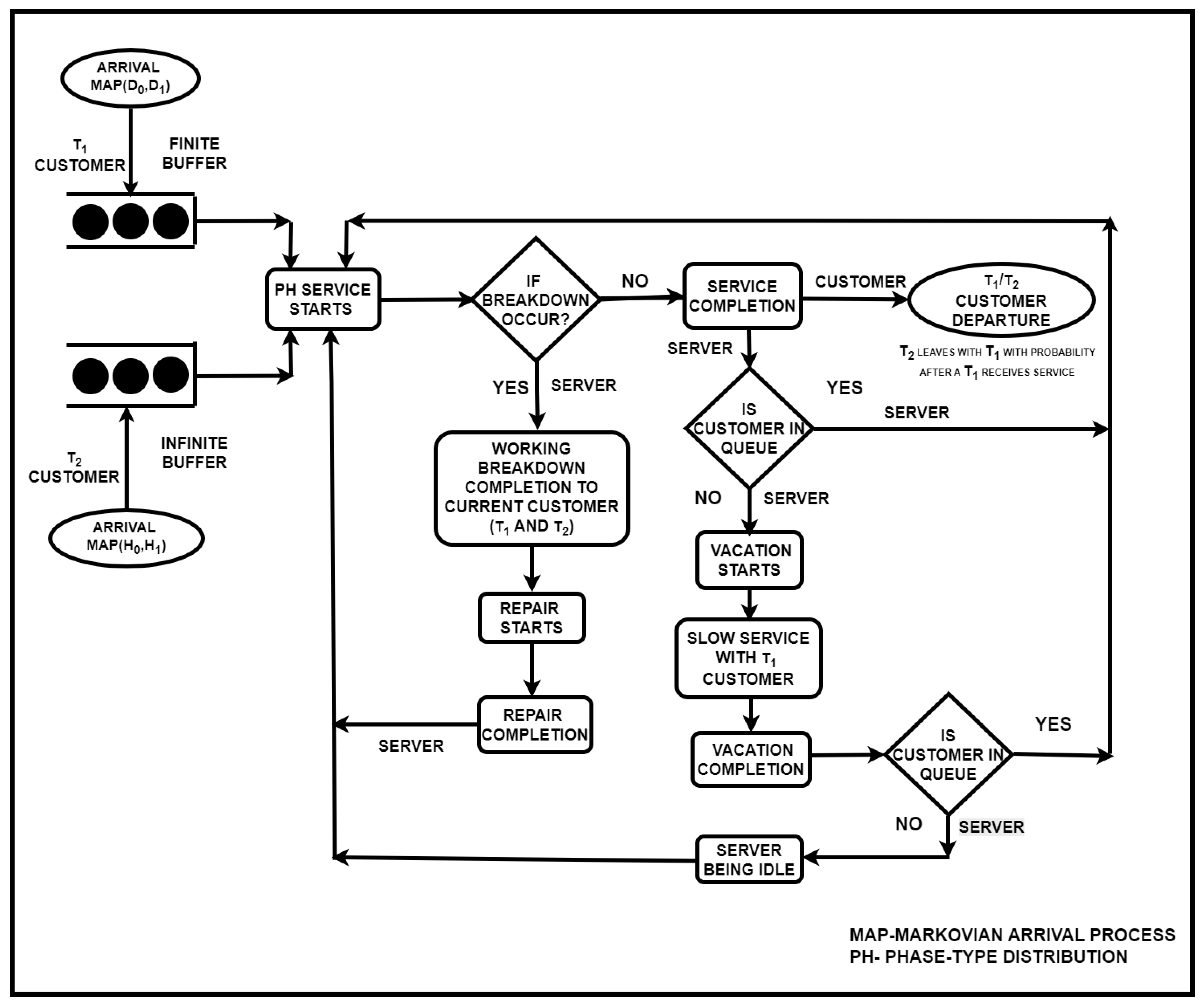
Figure 2.
vs. Service rate - ERA.
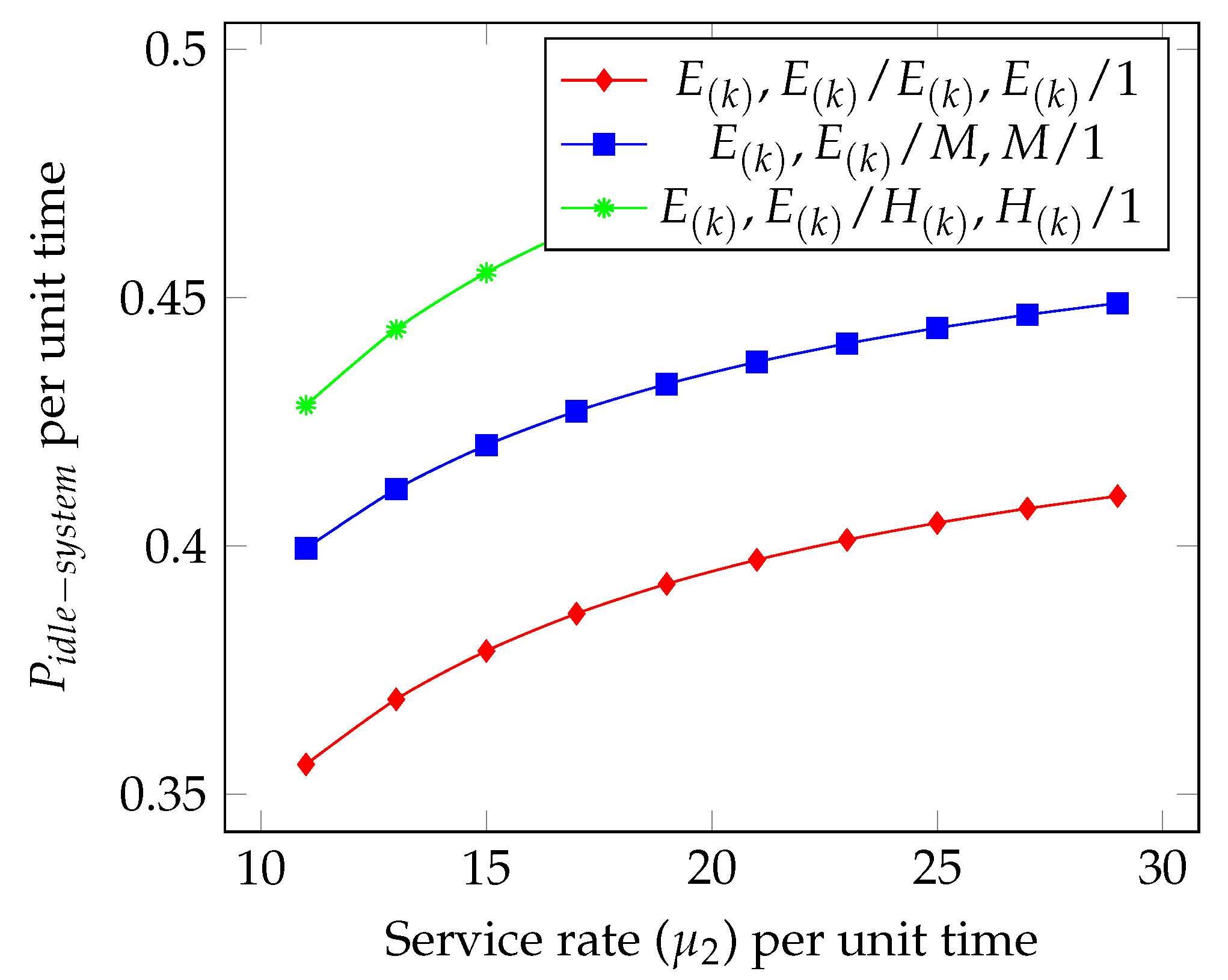
Figure 3.
vs. Service rate - EXA.
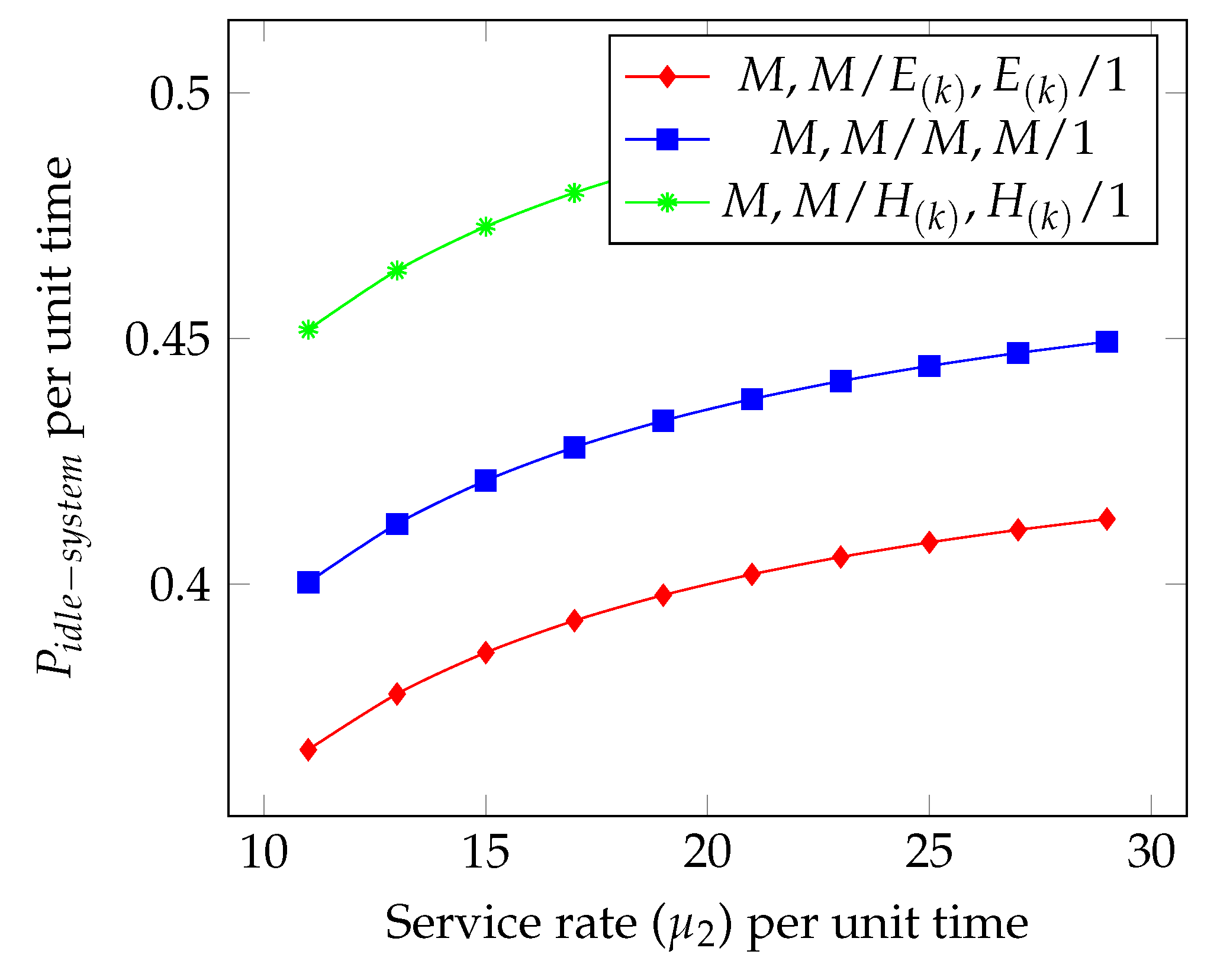
Figure 4.
vs. Service rate - HEXA.
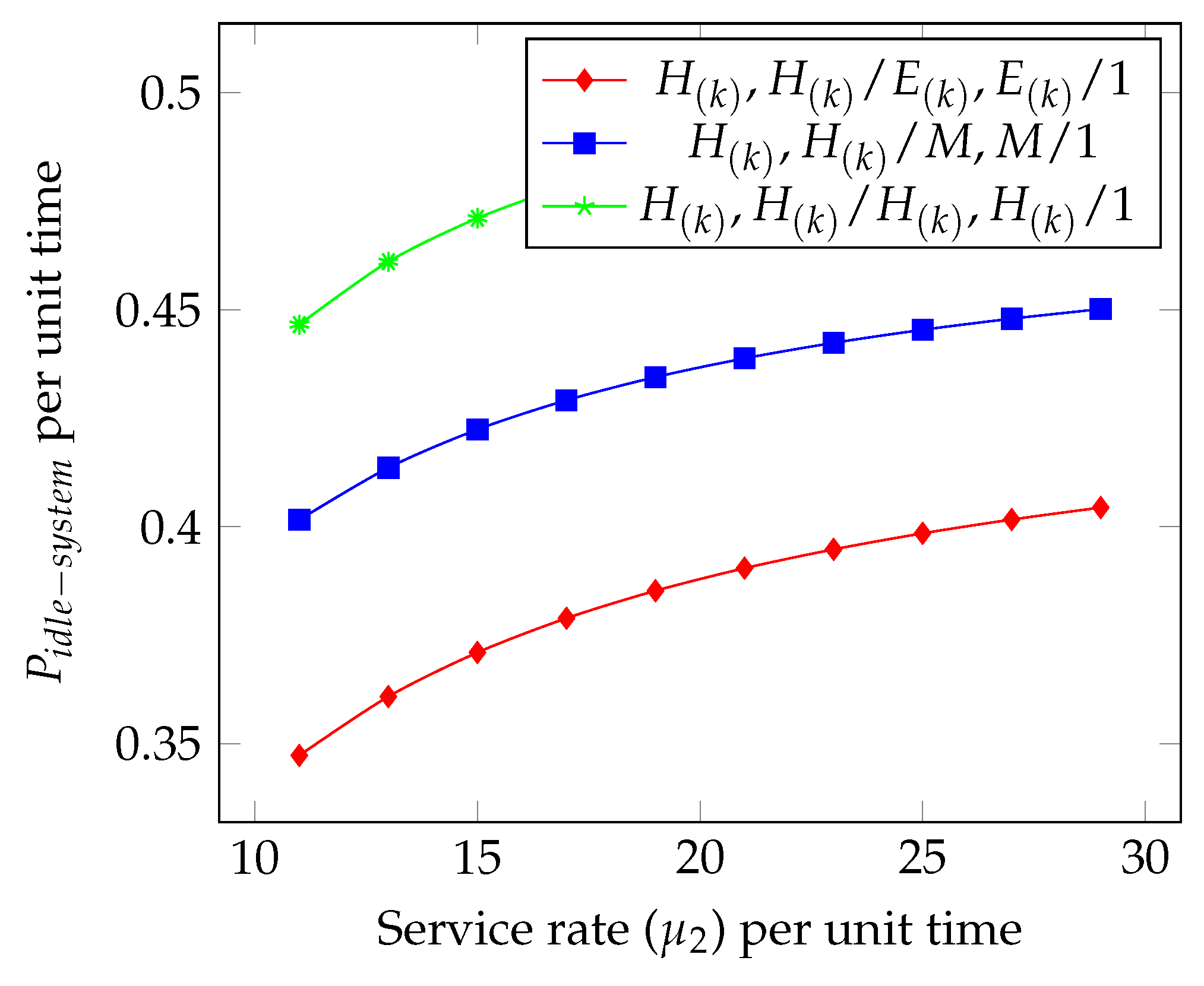
Table 4.
vs. service rate -.
| ERA | EXA | HEXA | |
| 11 | 0.062016 | 0.054459 | 0.048891 |
| 12 | 0.056528 | 0.049764 | 0.044835 |
| 13 | 0.051871 | 0.045785 | 0.041364 |
| 14 | 0.047881 | 0.042375 | 0.038368 |
| 15 | 0.044432 | 0.039423 | 0.035761 |
| 16 | 0.041425 | 0.036846 | 0.033473 |
| 17 | 0.038784 | 0.034578 | 0.031453 |
| 18 | 0.036448 | 0.032568 | 0.029657 |
| 19 | 0.034369 | 0.030775 | 0.028050 |
| 20 | 0.032508 | 0.029166 | 0.026606 |
Table 5.
vs. service rate -.
| ERA | EXA | HEXA | |
| 11 | 0.057451 | 0.054327 | 0.048716 |
| 12 | 0.052635 | 0.049782 | 0.044798 |
| 13 | 0.048525 | 0.045896 | 0.041416 |
| 14 | 0.044982 | 0.042544 | 0.038475 |
| 15 | 0.041901 | 0.039627 | 0.035901 |
| 16 | 0.039200 | 0.037068 | 0.033633 |
| 17 | 0.036815 | 0.034809 | 0.031622 |
| 18 | 0.034696 | 0.032800 | 0.029828 |
| 19 | 0.032800 | 0.031003 | 0.028220 |
| 20 | 0.031096 | 0.029388 | 0.026770 |
Table 6.
vs. service rate -.
| ERA | EXA | HEXA | |
| 11 | 0.047689 | 0.047659 | 0.062945 |
| 12 | 0.044663 | 0.044522 | 0.056734 |
| 13 | 0.041942 | 0.041719 | 0.051656 |
| 14 | 0.039491 | 0.039209 | 0.047412 |
| 15 | 0.037280 | 0.036952 | 0.043806 |
| 16 | 0.035278 | 0.034917 | 0.040699 |
| 17 | 0.033461 | 0.033074 | 0.037993 |
| 18 | 0.031806 | 0.031400 | 0.035614 |
| 19 | 0.030295 | 0.029875 | 0.033505 |
| 20 | 0.028911 | 0.028479 | 0.031623 |
Disclaimer/Publisher’s Note: The statements, opinions and data contained in all publications are solely those of the individual author(s) and contributor(s) and not of MDPI and/or the editor(s). MDPI and/or the editor(s) disclaim responsibility for any injury to people or property resulting from any ideas, methods, instructions or products referred to in the content. |
© 2025 by the authors. Licensee MDPI, Basel, Switzerland. This article is an open access article distributed under the terms and conditions of the Creative Commons Attribution (CC BY) license (http://creativecommons.org/licenses/by/4.0/).
Copyright: This open access article is published under a Creative Commons CC BY 4.0 license, which permit the free download, distribution, and reuse, provided that the author and preprint are cited in any reuse.


