

Submitted:
27 August 2024
Posted:
28 August 2024
You are already at the latest version
Abstract
In this paper, we investigate the equilibrium strategies for customers arriving at overtaking-free queueing networks and receiving partial information about the system’s state. In an overtaking-free network, customers cannot be overtaken by others arriving after them. We assume that customer arrivals follow a Poisson process and that service times at any queue are independent and exponentially distributed. Upon arrival, the received partial information consists in the total number of customers already in the network, however the distribution of these among the queues is left unknown. We prove the existence of equilibrium threshold strategies for such systems and provide methods to compute them.
Keywords:
overtaking-free networks
; equilibrium strategies
; Jackson networks
; tree networks
1. Introduction
This work aims to find the equilibrium strategy adopted by customers who arrive at an overtaking-free queueing network, under the assumption that, on their arrival, they are informed only about the total number of customers already in the system but not their distribution among the queues. The analysis of optimal strategies for queueing systems can be traced back since 1969, when Naor found the individual’s optimizing strategy that gives a rule for join or balk in the observable model [1]. This work was later extended by Edelson and Hildebrand in 1975, by looking at the unobservable model [2]. A nice recollection of results on queueing systems under the economical perspective, can be found in the recent monograph by Hassin and Haviv [3].
Since the 2000s, studies on partially observable models have intensified. In particular, regarding single service systems, this topic was discussed in 2007 by Guo and Zipkin, who looked at the effects on the model with: no information, partial information and full information [4], and, in 2008, by Economou and Kanta, who explored the single server Markovian queue with compartmented waiting space [5]. As for batch service queueing systems, in 2017, Bountali and Economou studied the strategic customer behavior for the observable and unobservable queue with single arrivals and batch services [6], and, in 2019, they extended this model, by considering the partially observable case, where the arriving customers observe only the number of complete batches that wait to be served [7].
While most of the above research on optimal strategies in queueing systems, refers to single queues, recently few results have been obtained about queueing networks. A first attempt has been done in D’Auria and Kanta [8], who analyzed the two-node tandem network and showed that a pure threshold equilibrium policy exists, assuming that arriving customers are informed only about the total number of users in the system. Later, Bara Kim and Jeongsim Kim generalized this result by considering multi-node tandem networks [9]. This work extends these results by focusing on the general overtaking-free queueing networks under partial information.
The class of overtaking-free networks appeared in the queueing context already in 1979, when Walrand and Varaiya proved that in an open multiclass Jackson network the sojourn times of a customer along an overtaking-free path are independent [10]. Kelly and Pollett obtained a similar result in 1983 analyzing closed Jackson network [11]. The overtaking-free condition ensures that no customer can influence the sojourn times of any other customer arrived earlier in the system. In this study, we characterize the topology of the FIFO overtaking-free networks with exponential service times, and show how to compute and optimize the profit function of partially informed arriving customers.
In the sequel, Section 2 contains the characterization of the overtaking-free networks, under the mentioned assumptions. In Section 3, we introduce the model and the notation. Then, in Section 4, we get the stationary distribution for the number of customers in the system in the unobservable and the observable case and compute the expected sojourn time at any queue given the total number of customers in the system. In Section 5, we derive the equilibrium threshold strategies. In Section 6, we provide some numerical computations by comparing two different queueing networks and finally in Section 7 we draw some conclusions.
2. Overtaking-Free Networks
In this section, we show that, under a FIFO discipline and with exponential service times, a necessary and sufficient condition for a queueing network to be overtaking-free is that the its underlying graph is an out-tree.
We define by the underlying finite directed graph of a queueing network. V represents the set of vertices, that correspond to the nodes where customers can queue up and receive their service. is the set of edges, that correspond to the allowed movements between queues and towards to the outside. We assume that and , where . We denote by the outside vertex, and we let and . Sometimes we refer to the graph with the intention to include the outside node inside the set of vertices . denotes the set of vertices, in , that are reachable from a vertex . After completing the service at queue , a customer either joins a queue among the nodes in or leaves the system, whenever . We let be the out-degree of vertex .
We assume that in the graph , the outside node can access and can be accessed by any node via a given path of edges. We also assume that the directed graph is connected, that is, for any non trivial subset , there exists an edge , such that either and or and . This implies that the network cannot be split into two separated sub-networks. If , we say that the graph (as well as ) is rooted. In this case, we assume that the root node is the vertex . The directed graph , with root vertex , is an out-tree if and, for any , there exists a directed path from 1 to v. It also holds that such a path is unique.
Now, we give a formal definition of overtaking-free network [10,11]. We have in mind that the outside node 0 is a source of customers. We can think of it as being a single server queue with infinite number of customers in its line. In general, we are going to assume that this source of arriving customers is stochastically modeled as a Poisson process. We then define a tagged customer as a customer that just left the outside node 0 to reach any node in the set , and that we are going to analyze.
Definition 1
(overtaking-free network). A queueing network is overtaking-free if and only if the sojourn times of a tagged customer at any queue along her path do not depend on the behavior of the customers arriving at the network at later times. That is, her sojourn times stay the same if no more customers are allowed to enter the network.
We define the following standing assumptions:
Assumptions 1.
- the inter-arrival times, the service times and the routing probabilities are independent random variables, whose distribution may only be node dependent;
- each node is a single server queue;
The above assumptions are implicitly assumed in the statement of the following theorem as well as for the rest of the paper.
Theorem 1
(Characterization of overtaking-free networks). Under the FIFO discipline and exponential service times at each queue, a necessary and sufficient condition for a queueing network to be overtaking-free is that its underlying graph is an out-tree.
Proof.
It is clear that if the graph is an out-tree and the service discipline is FIFO, then the network is overtaking-free. Indeed, each node would be reachable by a unique path, and along it, customers are served according to a FIFO discipline. On the other hand, assume that the network structure is not an out-tree, and consider two alternative paths joining two vertices . Then, there is a positive probability that two consecutive arriving customers go along the two alternative paths , where the arrows denote a sub-path between two nodes. Since the support of the exponential distribution is , there is a positive probability that the second customer, the one arrived later, will reach the node before the first customer, and will queue there in front of her. This would contradict the overtaking-free network hypothesis that the presence of the second user in the network should not alter the sojourn times of the first one. □
The previous proof would hold even if we substitute the exponential service distribution with any distribution whose support is unbounded or dense close to 0. However, in general, if we change the service discipline or the distribution of the service times, Theorem 1 may no longer be valid. One can easily construct counterexamples by using degenerate deterministic service times.
We conclude that, under a FIFO discipline and with exponential service times, in an overtaking-free network, node 1 serves as the root of the tree, and all other nodes have only one entering edge.
3. The Model
Under the assumption of exponentially distributed service times, an overtaking-free network is characterized by having a branching structure, described in Section 2, represented by its underlying graph that is an out-tree. A tandem network is a special subclass of overtaking-free network, and it has been studied in [8] for the case of two queues and [9] for a general finite number of queues. Here we extend those analyses to the whole class of overtaking-free networks.
The methodology consists in exploiting the product form expression of the stationary distribution of the network and comparing it with a closed one having the same number of customers inside as the one communicated to the tagged customer at the arrival epoch. We are allowed to make this comparison because all customers behind the tagged one can be overlooked under the overtaking-free assumption since they do not interfere in the calculation of her expected sojourn time.
Using this methodology, we compute a common equilibrium threshold strategy that all customers are going to implement in deciding whether to join or balk the system. This decision is only based on the partial information received at the arrival epoch, consisting in the total number of customers already inside the network.
The optimal strategy is computed by building an expected profit function P, that only depends on the number of users in the system and the common strategy followed by the rest of customers. The sign of the profit function corresponds to the decision of the tagged customes, she decides to join if the sign is positive, otherwise she decides to balk. Once joined the system, she is committed to her decision and cannot renege, and, if she chooses not to join, she will not have another opportunity to come back.
Finally, we verify that this optimal response leads to an equilibrium.
Consider an overtaking-free network and denote with the associated out-tree graph. Let and , so that N is the total number of queues, and , for , denotes the edge entering in node i, which we know to be unique.
Customers arrive at the network through node 1, according to a Poisson process with intensity and are served based according to a FIFO discipline. A customer completing her service at node , is routed to another queue at node with probability . Remember that 0, the outside node, may belong to allowing the customer to leave the network when served at node . The service times of customers at each queue are independent and exponentially distributed with mean .
Figure 1 illustrates an example of overtaking-free network.
4. Stationary Distribution
The only information that is provided to the customers at the moment of their arrival consists in the total number of customers in the system. Using this information they may decide to join the network or balk, and they may do it according to a strategy potentially random. It follows that we may represent a strategy, say s, as an infinite vector, that is ,where , is the probability that an arriving customer will join the system after observing a total number of k customers in it. In particular, for , we denote by , the K-threshold strategy, with the property that .
Remark 1.
We say that a strategy s is a pure strategy whenever for all . A K-threshold strategy is a pure strategy. We say that a strategy s is a mixed x-threshold strategy, where with and , if for , , and for . This means that an arriving customer certainly joins if there are less than n customers in the system, joins with probability p if there are exactly n customers, and otherwise she balks. A mixed threshold strategy is a convex combination of two pure threshold strategies, indeed .
We say that a strategy is admissible if whenever , for a given , then for any . In this case the number of customers in the network can be at most K and the network is called semi-open. If the strategy s is positive, that is for all , the network is said open and we set . To simplify the exposition, in the following when we say strategy we implicitly mean admissible strategy, and we denote by , the maximum number of customers allowed in the network given the strategy s.
Under the assumption that everyone uses the common strategy s, we denote by the expected potential profit function for an arriving customer that observes k users in the network, that is
where R is the positive reward for entering the system and is the expected cost for sojourn time. is the positive cost for unit sojourn time at queue i, also said cost rate, and is the expected sojourn time that a joining customer will spend at queue i, under the common strategy s and having received the information . is the corresponding sojourn time and denotes the total number of customers at her arrival time. The profit for balking is assumed to be 0.
In Section 5, we give an algorithm to compute , and find the equilibrium strategy by maximizing it under the assumption that all customers use the same strategy.
Thanks to the assumptions of independence and exponential service times, we can describe the dynamics of the network only by keeping trace of the number of customers at each queue, that is the vector . Indeed, the system can be described as a continuous time Markov chain with values in . In particular, this kind of network can be seen as a generalized Jackson network, whose special property consists in having a state-dependent arrival rate due to the joining strategy s; according to the nomenclature in [12], this network belongs to the class of Whittle networks. For a background on Jackson network, consult the Chapter 2 of [13], and for more general Whittle networks the book [12]. In our case the arrival rate is equal to , where is the total number of customers in the system, and is the maximum arrival rate, the one achieved if no customers would decide to balk.
A nice property of Jackson and Whittle networks is that the stationary distribution, when it exists, has the so-called product form, that is the queues behave like they were almost independent.
We denote by the solution of the normalized traffic equations, satisfying the normalizing condition and the following relation
We set with .
When the network is overtaking-free, and its graph is an out-tree, the solution of the traffic equations (2) are readily written. Indeed, denoting by the set of edges that belong to the unique path from node 1 to node , then and, for , , where for .
Let be a vector distributed as the stationary number of customers in the network, and let be the stationary distribution, so that , with denoting a general state.
It is known that in a Whittle network, with any topological structure, at most one transition by time may occur, and that the time between two transitions is exponentially distributed with state dependent rate. We define by the operator that moves one customer from node to node , that is , where , for , is the -dimensional unit vector with the i-th coordinate equal to 1 whereas . The transition rate from to , whenever , is
In an overtaking-free network, , however we keep the notation general as the stationary regime does hold for a more general topology.
Assuming that the stationary distribution exists, that occurs when the network is stable, it has the following form
In the sequel, we will not check the stability assumption as it always holds when . In (3), , and the missing normalizing constant is
To check that (3) indeed holds, one can verify that the global balance conditions are satisfied, see also Example 1.49 in [12].
In the following, we are also going to deal with networks whose number of customers inside is kept constant, say . In this case the network is called closed, and in it, transitions from/to node are not allowed, therefore the strategy employed by all customers is irrelevant. When the network is closed, the normalizing condition in (2) is substituted with . A closed network is always stable, and its stationary distribution has the following product form, compare with (3),
Denoting by a random vector distributed according to this stationary distribution, it has the same joint distribution as independent Geometric random variables with corresponding parameters conditioned to have a total sum equal to K.
Jackson and Whittle networks enjoy the MUSTA property (Moving Unit Sees a Time Average) at Simple Network Transitions, see Example 4.38 in [12], according to which, any customer moving, among the queues or from/to the outside sees, before joining the destination node, a stationary network having one less maximum number of customers.
To better formalize this property, we need to introduce the Palm probabilities. We consider the stationary network process , whose trajectories belong to the space of right-continuous functions with left limits with values in , and for fixed with , we define the set of simple network transitions from i to j as
Assuming the common strategy s, we denote by the state of the network at time 0 just before a customer, making a -transition, has joined her destination node, and we define its distribution. This distribution takes the name of Palm distribution, it has the special property to be conditioned to the occurrence of a -transition that is a null event, and it was first introduced by Palm in [14].
We give a heuristic proof of the MUSTA property in the following proposition, for a more formal proof see [12, Theorem4.37 & Example4.38].
Proposition 1
(MUSTA property). Fix , , and consider as in (5).
For a (semi-)open network employing the strategy s, and with denoting the shifted strategy, that is , then it follows that
where denotes the distribution of a similar network in which all customers employ the strategy .
If the stationary distribution refers to a closed network with a number of customers equal to K, in which the strategy s is irrelevant, the distribution refers to a closed network with number of customers.
Proof.
To simplify notation, we set and , for and . To compute , we do the following calculations,
where . To get the result for a closed network with K customers, it is enough to repeat the same reasoning above, after setting , considering and summing over . □
When , the -transitions correspond to the Poisson arrivals. This is the most recurrent case, and the property takes the well known name of PASTA (Poisson Arrivals See Time Averages), see [15]. We collect this fundamental result in the following corollary.
Corollary 1
(PASTA property). In stationary regime, an arrival customer sees an open network in a state distributed according to the stationary distribution, that is
If the network is closed (semi-open) with K (maximum) number of customers, in (7) refers to the stationary distribution of a similar network with (maximum) number of customers.
Thanks to the PASTA property, , where . In applying this formula, it is important to interpret the random variable as the sojourn time that a new customer, joining the queue with probability (in an overtaking-free network ), is going to spend in queue along her path throw the network. The total number of customers in the network, in case and after the new one has joined, is then .
Another property of a Jackson network with state-dependent arrival rate consists in the fact that, under the partial information , its stationary distribution coincides with the one of a similar closed network with k circulating customers. We collect this well-known result in the following proposition, noticing that its proof is an immediate consequence of the product form (3) and the definition of the conditional probability.
Proposition 2.
With being a random vector distributed as the stationary number of customers in a closed network with total customers, the following equality in distribution holds
Next proposition gives a known efficient algorithm to compute the expected number of customers, , at each node , see Section 2.5.5 in [13] for a proof.
Proposition 3
(Mean value analysis). The mean number of customers at node in a closed queueing network with customers, can be computed recursively according to the following algorithm
with .
Corollary 1 and Proposition 2 imply that an arriving customer that sees k customers in the system behaves in the same way as an arriving customer belonging to a closed network with customers. That is, before the arriving customer joins, the customers in the network are distributed as and just after joining they are distributed as .
Since the tagged customer is indistinguishable from all others, we can use the information about the distribution of the customers in the system to finally estimate her expected sojourn times at each queue.
Theorem 2.
In an overtaking-free network, assuming that the tagged customer only knows the total number of customers in the network at her arrival epoch, say k, independently of the common strategy s, her expected sojourn time at node is equal to
and it can be computed recursively by the formula and, for ,
Proof.
At the arrival epoch of the tagged customer, by the PASTA property (7), she encounters in the network a stationary number of users. Once she gets the information that the total number of users in the network is equal to k, the distribution of the customers in the network reduces to the one of a stationary closed network with k customers, according to Proposition 2.
After that moment, and assuming that she decides to join, by the overtaking-free condition, the future arrivals will not interfere with her future sojourn times she will spend at each queue along her random path throw the network. Therefore, we are allowed to change the future arrivals, so that we may assume that the network evolves as a closed network with customers in it. The tagged customer is then indistinguishable with respect to any other customer of this new closed network.
Looking now at the tagged customer as a typical customer in a closed network with customers, an application of the MUSTA property (6) implies that at any transition she will meet a network whose customers are distributed as a closed network with k customers inside. This allows to compute her expected sojourn time. Indeed, in a stationary closed network with k customers, these customers are distributed according to the distribution given in (4).
The tagged customer visits the node with probability , and it spends there a sojourn time equal to . We get that , with B an independent Bernoulli random variable with parameter and independent exponentially distributed random variables with parameter . By taking the expectation, (10) readily follows. Then using this formula and (9), we get (11). □
Remark 2.
A short observation about the use of the overtaking-free property in the proof of Theorem 2 is due, as it is subtle. Since the MUSTA property (6) holds for any Jackson and Whittle network, one would be tempted to believe that the overtaking-free condition is not required, and that also in a general network in which overtaking is allowed, one could easily compute the distribution or the expectation of the waiting times at each queue. The observation that should be made is that, in this case, the tagged customer would not be any more an indistinguishable customer belonging to her network. Indeed, at the moment of her entrance, she had an information more with respect to the others, that is, she knew that in the network there were exactly k customers circulating. However, she is not even belonging to a closed network because, due to the permitted overtaking, the number of customers ahead of her may change by some later arrival. Therefore, we are not allowed to apply the MUSTA property in the way we have done in the proof of the theorem.
Remark 3.
The result in Theorem 2 extends the one in [9], limited to tandem queues, to the more general class of overtaking-free Jackson networks with rate dependent arrivals. In [9], the strategy to compute the expected sojourn time in each queue, consists in using the Little’s law, that allows to get the value of for any . Then, by using the relation,
(Equation (4) in [9]), one can finally get the result given in (10). However, we point out that the Little’s law is very robust, meaning that it works in almost any queueing context, practically regardless of any distributional condition. This may misleadingly lead to believe that a similar result holds for more general tandem networks, or even for overtaking-free networks. However, this is not the case, see next Remark 4. Indeed, in order to make computable the expression in (12), one still needs that . This equality only holds for very specific models, such as the Jackson and Whittle networks that are very restrictive in terms of the distributions of their structural random variables. As a byproduct of the special properties of these networks, one also gets that .
Remark 4.
To be convinced that Theorem 2 makes strong use of the assumption of exponentially distributed service times, we recall here some counter examples. In particular, a single queue may always be seen as a tandem network with a single node, and consequently also as an overtaking-free network. In the literature, the single queue has been extensively studied, and in particular [16] has shown an example of M/G/1 queue that does not admit optimal equilibrium strategies. Moreover, the M/G/1 queue has been analyzed in full generality in [17], where it is shown that, depending on the service distribution, the equilibrium is not necessarily unique, and either the avoid the crowd phenomenon or the follow the crowd phenomenon may occur.
5. Equilibrium Strategies
Under an economic perspective, customers will join or balk the network according to an evaluation of their expected profit. Therefore, to look for the existence of an optimum equilibrium strategy, we need to study the expected profit function, in (1), of a tagged customer observing, at the arrival epoch, that the network already hosts k customers. We have omitted in the notation the explicit reference to the common strategy s, as it is actually independent of it, as shown more clearly below. The customer decides to join the system if and balks if , while she may take indifferently both actions when . This suggests that an optimal strategy would be a threshold one, that is , where K is the turning point of the sign of the function . In this section we are going to show that, indeed, this threshold strategy leads to an equilibrium.
We start by studying monotonicity properties of the cost functions appearing in (1) and computed in Theorem 2, by exploiting the ordering relations satisfied by the random variables as functions of k.
Lemma 1
(Stochastic ordering). The vectors are stochastic ordered in . That is, for any function non-decreasing in each coordinate,
Proof.
The proof relies on a coupling analysis, that is we construct on the same probability space two closed networks with respectively and customers, and show that the number of customers in each queue in the latter network is at least equal to the corresponding one in the former. The coupling is done by considering a closed network with customers inside, k of white color and one of red color. We also assume that the order of service is FIFO for the white customers, and preemptive resuming with low priority for the red customer. That is, the red customer is always pushed back at the end of the queue when there are some white customers at the same node, also when the red customer is the one in service, being alone, and a white customer joins the same node. It follows that the dynamics of the white customers are not affected by the presence of the red customer, in other words if we count only them in the network, they behave exactly as a closed network with k customers inside. On the other side, if we consider all customers, regardless of their colour, since the service times are exponentially distributed, they behave exactly as a closed queueing network of customers. Since the number of customers in each queue of the latter network is at least equal to the one in the former, counting only the white customers, the result follows. □
The monotonicity property proved in Lemma 1 immediately implies the following result on the expected sojourn times. It extends and corrects the results given in [8], see Appendix B.
Theorem 3
(Monotonicity of the expected sojourn time). For , the expected sojourn time at queue i, , is strictly increasing and as .
Proof.
The result follows by showing that, for , the variables are strictly stochastically ordered in k. We have that , with B an independent Bernoulli random variable with parameter and independent exponentially distributed random variables with parameter . Since is an increasing function of , the result follows by the stochastic order of the random variables proved in Lemma 1. The order is strict as while for any . The last result mentioned in the statement, follows by applying the L’Hopital’s Rule to the limit of the expression (10) as . □
By Theorem 2 and (1), we can compute the expected profit function in the following way
As anticipated,the profit function does not depend on the strategy s and of the arrival rate . Furthermore, by Theorem 3, is strictly decreasing in k and , which means that the benefit to join the network decreases as a function of the customers that are already inside.
It follows that at some point the function becomes negative, and we use this fact to show that there exists a common strategy, in particular in the class of threshold ones, that is optimal for all customers to implement.
Theorem 4
(Equilibrium strategies). Let be the threshold at which the profit function becomes negative. If , is the only pure equilibrium threshold strategy. If , the only equilibrium strategies are all the mixed threshold strategies , with .
Proof.
Assume that everyone else is using the strategy s, and consider a tagged customer that follows the strategy . Then her payoff, as a function of the customers she finds in the network is given by
and does not depend on the common strategy s. Therefore, by optimizing her profit, we get that the optimal strategy satisfies for and, assuming ,
That is, is an optimal strategy and since it is optimal independently of the common strategy s its also optimal against itself. In addition, if and , then also the strategy is optimal and an equilibrium strategy, as well as any convex combination of and . □
6. Numerical Computations
The easiest example of an overtaking-free network that is not a tandem network has an underlying out-tree with and . We compare this network with a two-node tandem network by looking at the equilibrium threshold strategies for different values of waiting costs per unit of time, as the routing probabilities vary. We refer to the first network with model A and to the two-node tandem network with model B.
As the Figure 2 shows, we choose for model A the routing probabilities , which imply and , and all service rates equal to . For model B (see [8]), we choose and , .
Both models have the first node equal, however in model A, after completing service at queue 1, customers are routed to queue 2 or queue 3 with equal probability and served there at rate while the customers in model B are all served at queue 2 but with twice the service rate, that is . In both systems, customers pay a cost C per unit of sojourn time at any queue.
We expect the equilibrium strategies to be similar to each other, due to the fact that, even if in model A queues 2 and 3 work at a speed that is half than the one of queue 2 in model B, they should handle, in a long run, half of the customers each.
Since both models have a simple topology we can get explicit formulas for the profit function as expressed by the following theorem.
Theorem 5.
The profit functions for the models A and B are respectively equal to
Proof.
For model A, we have that the vector is given by the truncation of a bivariate vector made of two independent random variables with distributions, respectively , and . Since , by Lemma A2 we have , and by (A5)
Then, having that , the relation in (15) holds.
The functions and are graphically represented in Figure 3a, where we fixed , and . Figure 3b shows the equilibrium thresholds as functions of . We observe that is slightly lower than and therefore the equilibrium thresholds in model A are generally lower than the ones in model B. This means that the customers in model A are more intimidated by the presence of customers in the network and decide to stop to enter for a less crowded network than the ones in model B. This is due to a well known fact in queueing theory, indeed model A is a less efficient network in that it wastes service capacity when one queue, among the queues 2 and 3, is idle while the other is working.
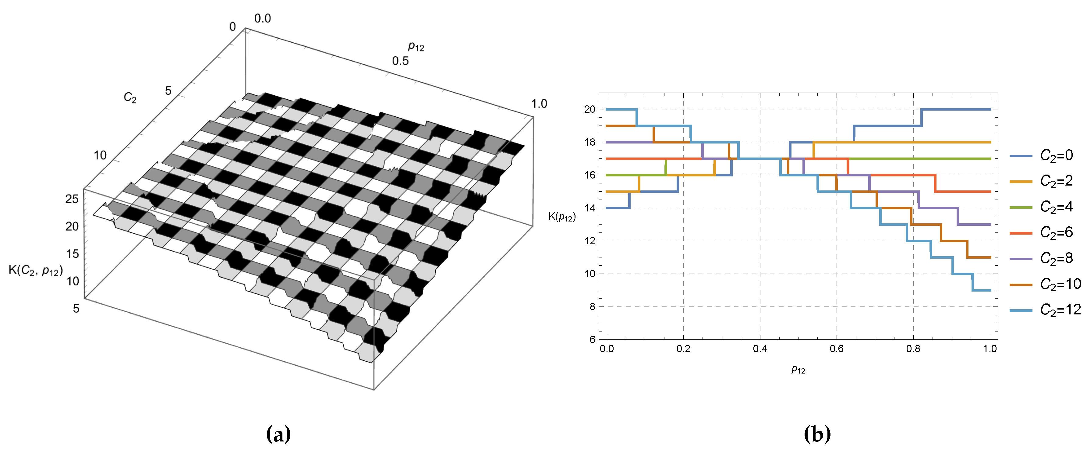
Now, we take a closer look at a variant of model A, by changing the routing probabilities and the costs for unit of sojourn time, in order to see how the equilibrium threshold are affected. We fix for , , , and we relax the assumption that . We assume that (i.e. ), with , and that (i.e. ) with . The values of the equilibrium threshold are represented in Figure 4. We observe that the thresholds are higher for low cost values and high probability values as well as for high cost values and low probability values. On the other side, they are lower when both and values are both high or low, forming a sort of saddle point in the middle.
7. Conclusions
The overtaking-free networks are special networks with the property that no customers entering behind a tagged one may influence her sojourn time in the network. Under the assumption of single server queues and exponentially distributed inter-arrival and service times, these networks are characterized by having an out-tree structure of the underlying graph.
For these networks, under the assumption that a tagged customer is informed about how many customers are already in the network at her arrival epoch, we compute the equilibrium strategies, that are shown to be of threshold type. Indeed, this follows by the fact that, under the partial information received by the arriving tagged customer, her sojourn times, as well as her profit function, do not depend on the common strategy used by the other customers.
Finally, we remark that the results heavy rely on the special property of the exponential distribution as there are known and easy to construct counter examples by using the simple M/G/1 queue.
Funding
The first and the third authors acknowledge the financial support by the Italian SID project BIRD239937/23.
Institutional Review Board Statement
Not applicable.
Informed Consent Statement
Not applicable.
Acknowledgments
The third author is member of the Istituto Nazionale di Alta Matematica (IN-dAM).
Conflicts of Interest
The authors declare no conflicts of interest.
Appendix A. Truncated Random Variables
In this section we describe some random variables that are obtained by truncated known discrete probability models.
Given a random variable , with probability mass function , we define the equilibrium rate of X the real-valued, non-negative function, for and with , see also [13].
The equilibrium rate function characterizes a random variable, as it is in a one-to-one relation with its probability mass function.
Let that , be the random variableX truncated at k, that is, its probability mass function is equal to , we notice that the equilibrium function of both random variable coincide up to k, that is .
We say that if it is distributed as the random variable truncated at . We have that , and
We also define the discrete Erlang distribution, that is constructed, similarly to its continuous counterpart, as the sum of independent Geometric distribution with the same parameter. That is, , for , if where are independent Geometric distributing with parameter .
In particular, we are interested in , with mean , and whose probability mass and equilibrium functions are given by
The corresponding truncated version has
We give now some results of marginal distributions of truncated vector of random variables.
Lemma A1.
Let be the truncation of a bivariate vector made of two independent Geometric distribution with parameters and respectively. Then its first coordinate, say , has a distribution.
Proof.
We need to prove that the equilibrium rate of is equal to . For , we have
□
Lemma A2.
Let be the truncation of a bivariate vector made of two independent random variables with distributions, respectively, and . Then its first coordinate, say , has a distribution.
Proof.
We need to prove that the equilibrium rate satisfies . For , we have
□
Appendix B. Note on D’Auria & Kanta (2015)
In [8], denotes the mean service time at the second station in a two tandem network with exponential service times with rates and . It is stated there that when , the function may be a decreasing function of the total number of customers in the network at the arrival moment of the tagged customer, i.e. k. This statement is false, according to Theorem 3.
In [8], the false statement is supported by a counterexample, that is expressed by a table showing the values of , for where the service rates are fixed to and . However, the values in the table are incorrectly calculated. Here we give the corrected table.
In particular, it is clear that it should always hold the relation .
| . | ||||||
It follows that, besides the statement of [8, Lemma 9] is correct, it is incomplete as is increasing for any value of the ratio , again according to results of Theorem 3.
References
- Naor, P. The regulation of queue size by levying tolls. Econometrica 1969, 15–24. [Google Scholar] [CrossRef]
- Edelson, N.M.; Hilderbrand, D.K. Congestion tolls for Poisson queuing processes. Econometrica 1975, 81–92. [Google Scholar] [CrossRef]
- Hassin, R.; Haviv, M. To Queue or Not to Queue: Equilibrium Behavior in Queueing Systems; Springer: New York, 2003. [Google Scholar] [CrossRef]
- Guo, P.; Zipkin, P. Analysis and Comparison of Queues with Different Levels of Delay Information. Management Science 2007, 53, 962–970. [Google Scholar] [CrossRef]
- Economou, A.; Kanta, S. Optimal balking strategies and pricing for the single server Markovian queue with compartmented waiting space. Queueing Systems 2008, 59, 237–269. [Google Scholar] [CrossRef]
- Bountali, O.; Economou, A. Equilibrium joining strategies in batch service queueing systems. European Journal of Operational Research 2017, 260, 1142–1151. [Google Scholar] [CrossRef]
- Bountali, O.; Economou, A. Equilibrium threshold joining strategies in partially observable batch service queueing systems. Annals of Operations Research 2019, 277, 231–253. [Google Scholar] [CrossRef]
- D’Auria, B.; Kanta, S. Pure threshold strategies for a two-node tandem network under partial information. Operations Research Letters 2015, 43, 467–470. [Google Scholar] [CrossRef]
- Kim, B.; Kim, J. Equilibrium strategies for a tandem network under partial information. Operations Research Letters 2016, 44, 532–534. [Google Scholar] [CrossRef]
- Walrand, J.; Varaiya, P. Sojourn times and the overtaking condition in Jacksonian networks. Advances in Applied Probability 1980, 12, 1000–1018. [Google Scholar] [CrossRef]
- Kelly, F.P.; Pollett, P.K. Sojourn times in closed queueing networks. Advances in Applied Probability 1983, 15, 638–656. [Google Scholar] [CrossRef]
- Serfozo, R. Introduction to Stochastic Networks; Springer New York: New York, 1999. [Google Scholar] [CrossRef]
- Chen, H.; Yao, D.D. Fundamentals of Queueing Networks; Springer New York: New York, 2001. [Google Scholar] [CrossRef]
- Palm, C. Intensity variations in telephone traffic. Ericsson Technics 1943, 44, 1–189. [Google Scholar]
- Wolff, R.W. Poisson Arrivals See Time Averages. Operations Research 1982, 30, 223–231. [Google Scholar] [CrossRef]
- Altman, E.; Hassin, R. Non-threshold equilibrium for customers joining an M/G/1 queue. Second International Symposium on Dynamic Games;, 2002.
- Kerner, Y. Equilibrium joining probabilities for an M/G/1 queue. Games and Economic Behavior 2011, 71, 521–526. [Google Scholar] [CrossRef]
Figure 1.
An example of overtaking-free network, with and , with , and , .
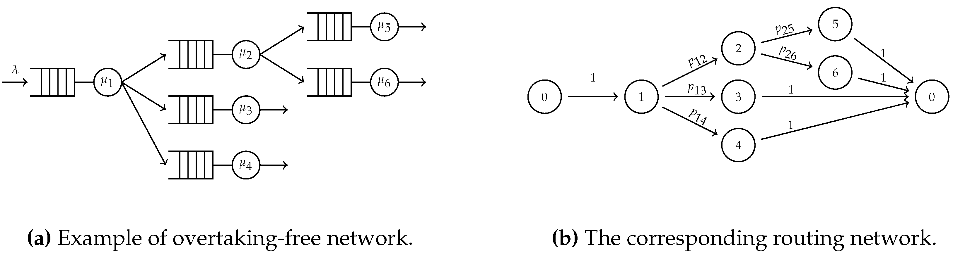
Figure 2.
Network representations.
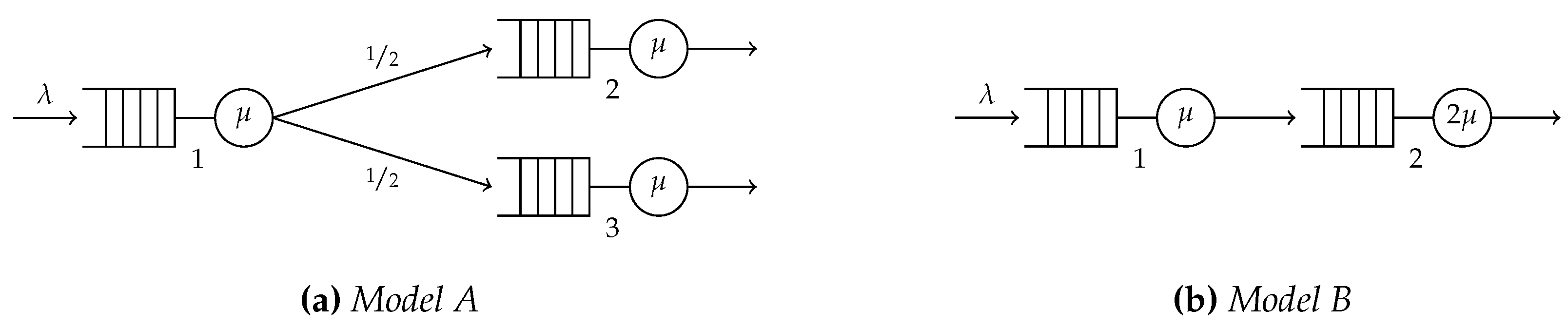
Figure 3.
Comparison between model A and model B with parameters , .
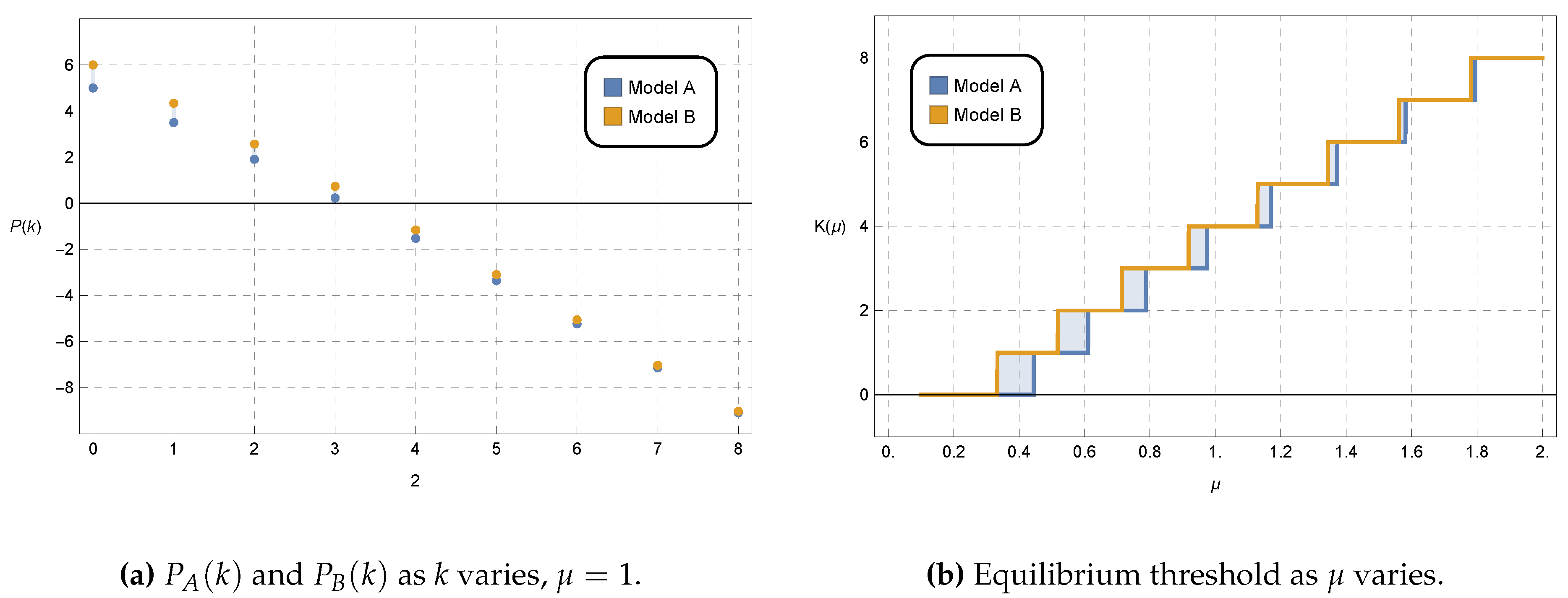
Figure 4.
Plot and show the equilibrium thresholds as a function of the routing probability and the cost , with , , , and .
Figure 4.
Plot and show the equilibrium thresholds as a function of the routing probability and the cost , with , , , and .
Disclaimer/Publisher’s Note: The statements, opinions and data contained in all publications are solely those of the individual author(s) and contributor(s) and not of MDPI and/or the editor(s). MDPI and/or the editor(s) disclaim responsibility for any injury to people or property resulting from any ideas, methods, instructions or products referred to in the content. |
© 2024 by the authors. Licensee MDPI, Basel, Switzerland. This article is an open access article distributed under the terms and conditions of the Creative Commons Attribution (CC BY) license (http://creativecommons.org/licenses/by/4.0/).
Copyright: This open access article is published under a Creative Commons CC BY 4.0 license, which permit the free download, distribution, and reuse, provided that the author and preprint are cited in any reuse.


