
Submitted:
12 November 2025
Posted:
13 November 2025
You are already at the latest version
Abstract
This study develops an environmentally sustainable inventory system for retailers engaged in the sale of recycled plastic products derived from the reprocessing industry. The model integrates an investment framework in additive manufacturing technology aimed at minimizing emissions and waste during production while simultaneously enhancing product quality. The main objective of the proposed inventory system is to elevate the quality standards of recycled products and improve overall profitability. Furthermore, the model incorporates demand-dependent reliability, pricing, and quality factors to maximize profit while satisfying customer demand. It also considers deteriorating items, potential shortages, and trade credit policies to ensure a realistic operational structure. The applicability and efficiency of the proposed proposal have been exhibited through a case study involving an existing retailer, confirming its capability to enhance profitability while promoting eco-friendly production through additive manufacturing. The results indicated that the incorporation of additive manufacturing technology led to more than 2% improvement in total profit for the inventory system. Moreover, a sensitivity analysis was conducted to assess the influence of key parameters on the optimal solution.
Keywords:
quality
; delay payment
; 3D-printing technology
; sustainable
; shortages
1. Introduction
As the world grapples with the mounting issue of plastic waste, innovative approaches are essential to mitigate the environmental impact of plastic products. One such approach is to leverage additive manufacturing (AM) or 3D printing technology to create innovative and high-quality products. Use of AM not only reduces the need for new production but also supports the principles of the circular economy and reduces waste on the environment. This offers precise control over material properties and product design, enabling the creation of customized and high-performance products made from recycled materials over traditional methods. [1] analysed various AM technologies that offer a significant advantage in reducing product development timelines for intricate structures. Furthermore, researchers discussed layer-by-layer additive process ensures high precision, enhancing manufacturing quality and reliability ([2,3]) and design an optimized, sustainable reverse logistics model for PVC recycling that minimizes costs and environmental impacts while improving operational efficiency. As AM integrates into manufacturing, its efficiency, sustainability, and adaptability reshape industries, promising a future marked by reduced waste, optimized inventory, and elevated production standards.
In the inventory system, one of the important parameters known as demand must be considered when making decisions about the stock and output of the warehouses. Researchers are emphasizing pivotal factors in inventory systems, notably focusing on aspects such as degradation, demand dynamics, and the assurance of reliability and quality. One of the significant challenges confronting the community today is the recycling of plastics by developing innovative and sustainable recycling with minimal environmental impact. In most of the research, facts are needed to answer the specific queries on inventory regarding AM as follows:
- Need to answer approaches to improve the quality of recycled products using additive manufacturing technology.
- How can a sustainable recycled inventory system be created through the use of AM technology?
- Analysis on investment from retailers in 3D printers can support the production of recycled products.
- How can the reliability of recycled plastic products be ensured while maximizing overall profit?
Retailers aim to maintain high-quality and eco-friendly products to meet customer demands within their inventory systems, driving a growing interest in sustainable and innovative manufacturing practices. Recycling plastic products, although vital for environmental sustainability, often leads to reduced product quality, reliability, and profitability. This study developed an Economic Order Quantity (EOQ) model by investigating sustainable strategies to enhance the quality and reliability by mitigating the waste, emissions, quality and reliability issues associated with recycled plastics. Furthermore, this advancement has motivated retailers to invest in 3D printing technologies, fostering the broader adoption of AM for sustainable and efficient inventory systems.
2. Literature Review
Nowadays, the majority of buyers prefer the acquisition of high-quality and dependable. Different scenarios in production inventory models have been analyzed that focus on particular situations incorporating demand affected by both price and inventory levels, decay of products ([4]), stochastic demand ([5]), and product reliability ([6]). Researchers ([7,8,9]) explored preventive maintenance strategies for manufacturing systems deteriorating in reliability and quality, assuming constant demand or the demand rates that vary with both stock levels and time [10]. Research has been developed on an inventory framework that incorporates fuzzy demand subject to price discounts ([11]) and also the considers sales price of the product ([12,13,14,15]).
The degradation rate significantly influences the optimal policy ([16,17]). Plastics degrade over time due to factors such as temperature, humidity, light exposure, and chemical interactions with other substances. Many researchers ([18,19]) have been studying inventory models for decaying items in recent years on the smart manufacturing system of degrading products through the application of preservation technologies. Numerous researchers ([20,21]) have created inventory models for perishable items with varying decay rates instead of a steady deterioration rate.
In industry, payment delay refers to the time it takes a company to settle a bill after receiving it, whereas late payments refer to payments that are delayed beyond the agreed-upon date. Several findings suggest that policies allowing for payment delays can result in heightened demand ([22,23,24]), whereas prepayment policies tend to diminish demand, depending on the duration of the prepayment terms ([25,26]).
Inventory shortages occur when demand exceeds available stock, leading to lost sales, reduced customer satisfaction, and reputational risks. To mitigate these challenges, advanced inventory management uses data-driven strategies like demand forecasting, safety stock optimization, and real-time tracking to minimize stockouts and improve efficiency. [27] created a sustainable inventory model with complete backlogs. developed a bi-objective model to make supply chains sustainable by minimizing production waste and reducing environmental emissions.
The implementation of AM technologies in inventory models for enhancing defect-free production, life cycle, and cost-controlled inventory reduces the environmental impact ([28]) irrespective of the kind of material and production process. [29] created a life cycle inventory framework for stereolithography, a commonly employed AM method. [30] developed an environmental evaluation of an AM method that used a generic framework to examine the ecological impact of 3D concrete printing via a parametric approach. [31] developed a bi-objective sustainable supply chain for reduce waste generation and pollution through the integration of AM. [32] reviewed the use of recycled polymers in 3D printing, emphasizing recycling methods, reinforcements, and parameter optimization for sustainable production. AM technology has been designed for strategies in supply chain network ([33]), conventional warehouse inventory system ([34]), and also on the inventory model ([35]) so that businesses may enhance. Researchers investigated and compared the effects of the incorporation of AM technology into the supply chain networks ([36,37,38,39,40]).
Research aperture on the topic:
This study further contrasts traditional manufacturing methods with AM technology within the inventory framework. There is a notable gap in addressing the integrated sustainable inventory model formulated to enhance the quality and reliability of recycled products using AM technology. This innovative model incorporates realistic factors such as price, time, quality, reliability demand, delayed payment, investment in AM technology, etc., aiming to achieve sustainable development. The present work aims to address the stated research gap by pursuing the following objectives:
- To develop a sustainable EOQ model integrating AM (3D printing) for eco-friendly inventory management.
- o enhance product quality and reliability while utilizing recycled plastic materials in production.
- To evaluate the economic and environmental benefits of adopting 3D printing technology in retailer operations.
Table 1 highlights the research gap and emphasises that this article is a pioneering effort to address all of the factors discussed collectively. More specific contributions to this manuscript are as follows:
- Introduce the additive manufacturing technology investments to increase the quality, reliability, and profitability of recycled products.
- A sustainable inventory model using AM technology for emission reduction and waste minimization to enhance the quality of recycled plastic products.

Table 1.
A contribution-oriented comparative analysis of the present study against earlier models.
| Reference |
Sustainable |
EOQ |
Price dependent demand |
Time dependent demand |
Quality dependent demand |
Reliability dependent demand |
AM Technology or 3D printing technology |
Delay payment |
| [41] | × | × | × | × | × | × | ✓ | × |
| [42] | × | ✓ | ✓ | × | × | × | × | × |
| [43] | × | ✓ | ✓ | × | × | × | × | × |
| [44] | × | × | ✓ | × | × | × | × | × |
| [45] | ✓ | × | × | × | × | × | ✓ | × |
| [46] | × | ✓ | ✓ | ✓ | × | × | × | × |
| [47] | ✓ | × | × | × | × | × | ✓ | × |
| [48] | × | ✓ | ✓ | × | × | × | × | × |
| [49] | × | × | × | × | × | × | ✓ | × |
| [50] | ✓ | ✓ | ✓ | × | × | × | × | ✓ |
| [51] | ✓ | × | × | × | × | × | ✓ | × |
| [52] | ✓ | × | ✓ | × | × | × | × | × |
| [53] | × | ✓ | ✓ | ✓ | × | × | × | ✓ |
| [54] | ✓ | ✓ | × | × | × | ✓ | ✓ | × |
| [55] | × | ✓ | ✓ | × | × | × | × | ✓ |
| [56] | ✓ | ✓ | × | ✓ | × | × | × | ✓ |
| [57] | × | × | × | × | × | × | ✓ | × |
| [58] | × | × | × | ✓ | × | × | ✓ | × |
| [59] | ✓ | × | ✓ | × | × | × | × | × |
| [60] | × | ✓ | ✓ | × | × | × | × | × |
| This paper | ✓ | ✓ | ✓ | ✓ | ✓ | ✓ | ✓ | ✓ |
3. Development of Sustainable Inventory System
This study is consistent with a negligible replenishment rate of the horizon for inventory planning that extends infinitely. The following considerations are essential and consistent with the review of this study.
- The demand rate for this model which depends on the price, reliability and quality and increases with time i.e., , here a is initial demand.
- Degradation initiates immediately upon lot reception, and its rate remains constant at deterioration rate denoted by .
- If the retailer settles the payment within the designated credit period D provided by the supplier, they will avoid any interest fees. Conversely, if the retailer makes the payment after the the credit term D, they will incur interest at the rate .
-
In case-I: When the stock duration is consistently positive and exceeds the credit term D (i.e., ). The consumer seeks to generate interest at an annual rate of . This situation arises when the credit duration D exceeds the duration of the stock. Using the sales revenue, calculate . After the credit period concludes, the unsold inventory will be financed at an annual rate of once the credit time has expired.Case-II: If the amount D equals or exceeds the allowable payment delay (i.e, ), the consumer is excused from paying interest and instead accumulates interest at a constant yearly rate within the range (0, D). This occurs if D is greater than , which indicates that D exceeds the allowable payment delay.
- The rate at which this model is in demand relies on product reliability, expressed as . The reliability of products offered by the retailer is influenced by the quality of goods provided by the manufacturer.
- Quality of items in the inventory system is i.e of quality item’s present in the inventory. Here is the amount of recycling products when 3D technology is investmented, and e is the efficiency of 3D technology in recycling products. The quality q = 0, when A = 0, and tends to when . The cost function of investment, q(A) is possesses continuous derivatives
Let is the starting point for the inventory level. As a result of demand and deterioration, the inventory level drops. Figure 1 shows two subperiods of T, when the inventory level drops to zero at time , there are shortages in the fully backlogged period .
with the condition and is continuous at
4. Derivation of Costs of Inventory System
The cost interpretation of a business framework is vital to deciding the system’s endeavour for an inventory model with a supplier or manufacturer.
Ordering cost : A constant expense associated with processing each order cycle, as given by
Holding cost ( unit per unit time): It refers to the costs or losses incurred by a business for maintaining inventory over a specified duration. Using expressions for appropriately by referring to Eq.-(3), the cost of holding for the sellable inventory is expressible as
An organization’s purchasing cost ( per unit time) is the amount it spends on purchasing the products and services it needs to operate or produce a product.
Purchasing cost (): The total cost expended by the merchant throughout the whole planning cycle for acquiring the requisite quantity of product in the form of purchase amounts is
The shortage cost () represents the expenditures or losses incurred by an organization due to insufficient inventory or product availability for customer demand, resulting in missed sales opportunities or customer dissatisfaction, which is evaluated as
Sales revenue: The total amount of money that the inventory system will make from the sale of goods throughout the planning cycle is provided by
Deterioration cost ( of deterioration per unit over time): From the stock that the retailer receives in excellent condition, a certain percentage of the items begin to deteriorate over time; as a result, the cost of deterioration is calculated as:
The AM technology investment cost per cycle is given by
Delay Based Payment Frameworks
There are two possible results from this inventory system: either the buyer’s conditional payment delays are larger or shorter than the cycle time. In order to determine the overall inventory costs, we evaluate the interest paid in both situations due to payment delays.
Case I: payment delay is less than the cycle time:
The interest earned from 0 to is provided by
The retailer’s cycle-specific interest rate is calculated by
In case , the total inventory cost per unit of time is calculated as .
Case II:() payment delay is greater than the cycle time:
Here is the retailer interest earned per cycle at the return rate. If , per cycle’s annual interest is given by
In case (), the total inventory cost per unit of time is calculated as
The total profit of the inventory system assessed per unit of time throughout the planning cycle for both the payment delays channel in AM technology expenditure.
5. Methodology
This section examines the optimal solution for sustainable inventory management, focusing on investments in additive manufacturing technology and credit options.
A function denoted as , is strictly pseudo-concave under the condition that not only is the function I(t) differentiable but also strictly concave. Additionally, J(t) is infinite and strictly adheres to this characteristic. The outcome is derived from the analysis of the function .
Theorem 1.
If . The Hessian matrix pertaining to demonstrates negative definiteness, thereby establishing that achieves a global maximum at the coordinates . Importantly, the coordinates represent a singular and unique point of attainment.
Proof.
: Let us consider
and
Partial differentiation with respect to both and T of the Eq.-(20)
Again, partial differentiation concerning both and T of Eq.-(21), we can derive
and
By taking the partial derivative of Eq.-(19) with respect to T, we can deduce
Taking the partial derivative of Eq.-(24) with respect to T allows for the derivation of
The Hessian matrix for is given by . The first principal minor is:
Even more, the second principal minor is : =
.
The second principal minor is >0 only if .
Given that and , the function exhibits strict concavity and differentiability. Moreover, represents a strictly positive affine function. According to theorem 3.2.5 from [61], attains the global maximum value at a specific point under the specified conditions, denoted as This concludes the proof. □
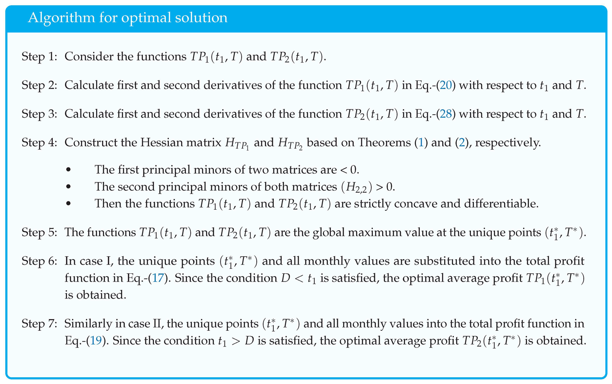
Theorem 2.
If . The Hessian matrix associated with consistently exhibits negative definiteness, signifying that it attains its global maximum at the singular point , and this extremum is unique.
Proof.
: Let us consider
and
Using partial differentiation with regard to and T of Eq.-(28), one can derive
Using partial differentiation with regard to both and T of Eq.-(29), we can find
and
By partially differentiating Eq.-(28) with regard to T, we can obtain
Taking the partial derivative of Eq.-(32) with respect to T , can derive
Now the Hessian matrix of is given by . The first principal minor is:
=
The second principal minor is positive >0 only if
.
Since and , the function is both strictly concave and differentiable.
In addition, the function is strictly positive and affine. Based on theorem 3.2.5 of [61], attains its global maximum at the unique point determined by the necessary conditions, specifically, it is This concludes the proof. □
6. Numerical Illustration
This section presents a case study of a retailer implementing 3D printing technology to manufacture products from recyclable plastic, with a focus on enhancing product quality and reliability and environmental considerations. To assess the effectiveness of the proposed inventory model, realistic operational data reflecting typical industry conditions are used, demonstrating how the model supports informed decision-making and improves overall operational performance. This approach highlights the model’s practical relevance and applicability. The conceptual framework, illustrated in Figure 2, depicts the retailer’s inventory system, emphasizing investment in 3D printing to transform recyclable plastic into high-quality products while simultaneously increasing profitability.
Consider the various types of cost components that retailers can use to develop a sustainable inventory system. Examine the different cost components incurred by the retailer in establishing a sustainable inventory management system.
The retailer spends for cost per purchasing unit item is , ordering cost per order is , cost of selling unit item is p is , holding cost per unit time per unit item is , shortage cost per unit time per unit item is and deterioration cost per decaying goods per unit per unit time is . The initial deterioration rate of the system is . The demand function having initial demand a is 100, , , the coefficient of price sensitivity b is 0.5, AM investment for quality products A is $5, efficiency of the AM technology e is 0.9, amount of recycling products is 0.9, supplier’s quality of the products s is 0.9 and .
The system under examination incorporates delay payment, wherein the retailer accrues interest at a rate of , while the supplier incurs an interest cost of . The comprehensive inventory system is evaluated over the course of a full year. Upon substituting all pertinent values into (16) and (18), the optimal value and total profit are derived. Table 2 delineates the optimal average profit corresponding to distinct payment delays in both scenarios. Let the supplier arrive with five options such as within (i) three months, (ii) five months, (iii) seven months, (iv) eight months, and (v) nine months.
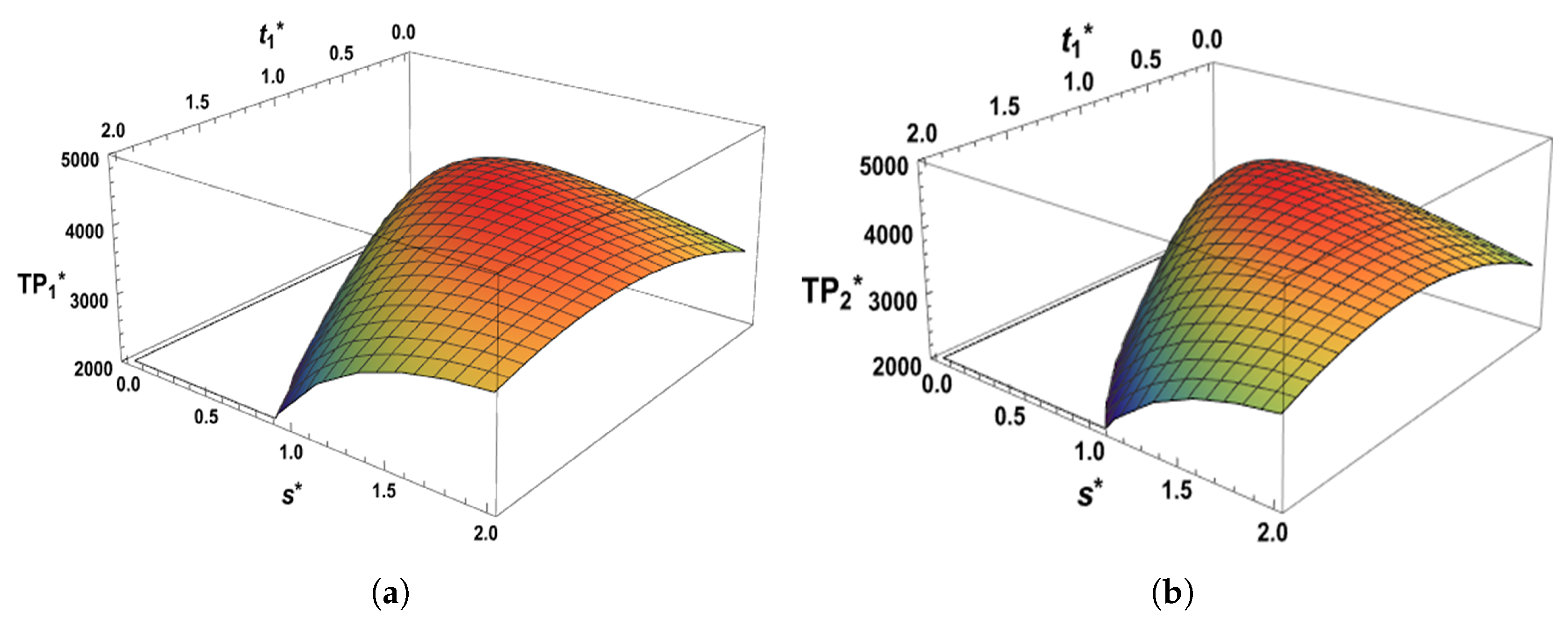
Table 2 shows that initially, with a three months payment delay (i.e., D=0.25), it is observed that and , which means that case-II is conflicting and only case-I holds with as the maximum average profit. Once more, with payment to the supplier occurring after five months (M=0.4165), the inventory model adheres to the condition that and . Consequently, only case-I is applicable, allowing the attainment of the maximum average profit . For the third case, where the supplier is paid after seven months (M=0.5833), the inventory model follows the fact that and therefore, here both cases are satisfied, so the result provided the maximum average profits and are possible. For the fourth and fifth cases, the inventory model holds only Case-II for the supplier receives payment after nine months (M=0.75) and eight months (M=0.6667), respectively, thus satisfying only Case-II. Consequently, the model adheres to this condition, maximizing the potential for the highest average profits, . The blue-coloured row Table 2 signifies the optimal solution for the inventory system. The concave representation of the optimal total profit under AM technology investment is shown in Figure 4 for and .
Figure 3.
Exhibit dependence of product quality on the investment level.
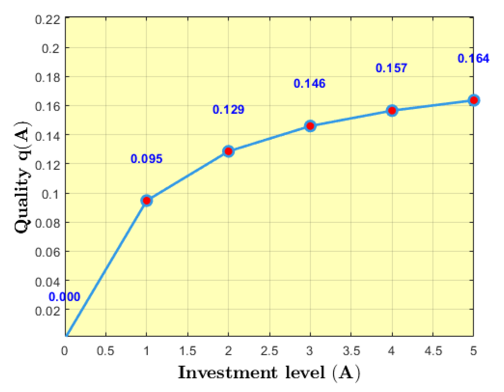
Table 3 presents a comparative analysis of the retailer’s optimal results with and without investment in AM technology. It can be observed that when the retailer incorporates AM particularly 3D printing to enhance product quality and reliability, the total profit increases notably. This improvement arises because AM enables the production of parts with higher precision, reduced defects, and better material utilization, leading to greater customer satisfaction and repeat demand. Although the production cycle time slightly decreases due to improved process efficiency, the profitability remains consistently higher compared with the conventional recycling approach.
7. Sensitivity Analysis
The purpose of this investigation is to examine the behaviour of parameters and to evaluate the applicability of theoretical findings in the context of recycling plastic products in companies or industries. Implementing a 3D technology-based inventory model has as its primary objective to maximize profits through cost reduction, as well as the improvement of product quality and reliability. The analysis will consider the observed variations in these parameter values , , , , .
From Table 4, it is noted that the ordering cost of the sensitivity is high. If ordering cost,the times and are increases and the total profits and are decreases, mean while the time and are increasing the total profits and are decreasing. The holding cost is less responsive to overall profit than cycle times. Increases in the holding cost result in a simultaneous decrease in both overall profit and cycle duration, a prevalent phenomenon frequently observed in the domain of inventory management.
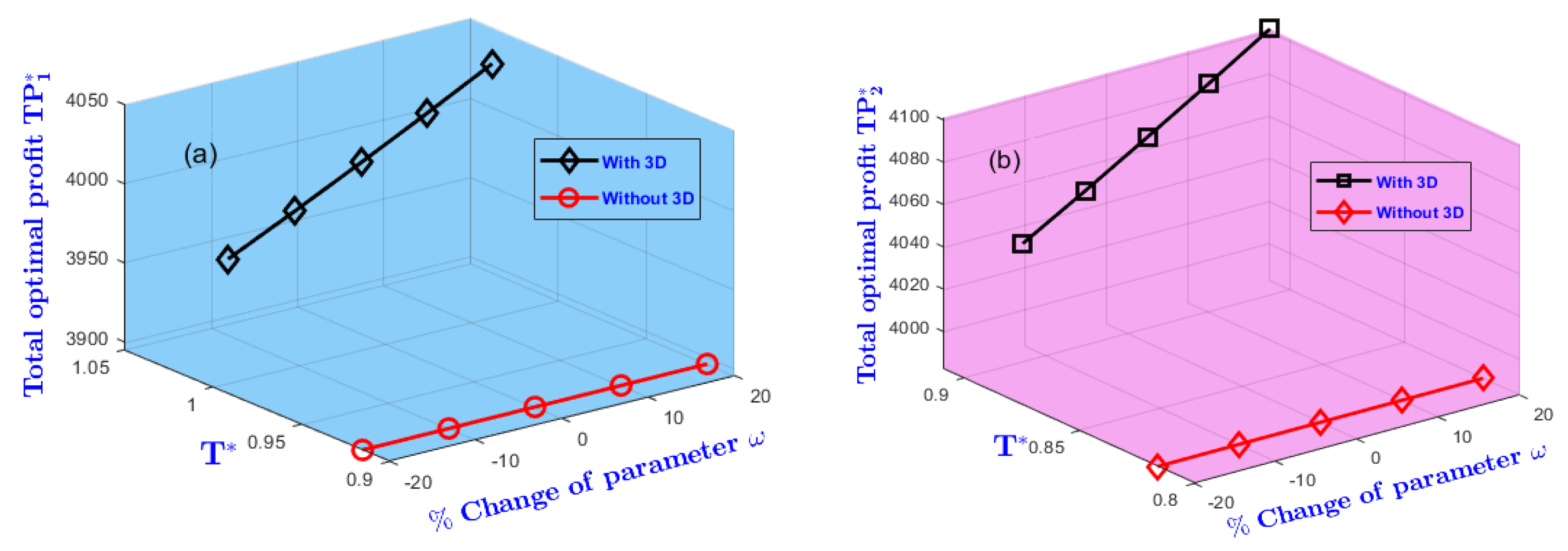
According to Figure 5, the comprehensive revenue of the inventory system exhibits a high sensitivity to the purchase cost , and the total profit is lower. If the inventory system’s purchasing cost rises, the overall profit falls, and the cycle duration shortens slightly in two scenarios, as shown in Table 4. The supplier selection issue is essential since the overall profit is more vulnerable to the cost of purchases. The store could choose a supplier who can provide goods at a lesser cost and make more revenue. The overall profit is less sensitive to ordering and deterioration costs, as seen in the table. Another practical alternative is investing in technologies that reduce the expenses associated with ordering and degradation.
The overall profit is less sensitive to shortage costs. Table 4 reflects that the total profit is decreases with variations in time and , displaying both increases and decreases. Concurrently, the total profit exhibits a reduction with alternating increases and decreases in the time parameters and . The impact of cost parameter sensitivity, specifically in relation to the investment in AM technology, results in a higher total profit compared to the sensitivity observed without such investment, as depicted in Figure 5.
The sensitivity analysis in AM technology-related parameters from Figure 6 the parameter increases is the amount of recycled products after AM investment the total profit will be increased. The above Table 5 shows decreases in the amount of recycled products after AM investment; the total profit will be less. The plastic recycling sector has the potential to create high-quality recycled goods through the use of AM technology. This approach not only boosts the volume of recycled materials following investment in AM but also contributes to lowering emissions.
Figure 5.
Impact of cost parameters on total optimal profit incorporating delay payment scenario for with and without AM technology.
Figure 5.
Impact of cost parameters on total optimal profit incorporating delay payment scenario for with and without AM technology.

Figure 6.
Sensitivity of total optimal profits by investing in AM technology to recycling rate (). Figure 6(a) and Figure 6(b) represents for with and without AM technology by and , respectively.
Increases the efficiency of the AM technology e the total profit will be increased. The above Table 4 shows the decreases in the total efficiency of the AM technology; the total profit will decrease. Sensitivity of the efficiency of AM technology parameter is shows in Figure 7 for total optimal profits. Increasing efficiency can help the plastic reforming industry increase profits. Using AM technology, recycled plastic objects can be manufactured with higher quality.
Increases the investment of the AM technology automatically increases the quality of items in the inventory production system, and it will obtain high profit. The investment parameter A decreases automatically, the quality of the item will decrease, and the profit will decrease. Therefore, the plastic reforming company utilises AM technology to improve product quality and boost industrial profits. The graph illustrates the overall optimal profit for both cases in Figure 8.
Increases the supplier’s quality of the products s the total profit will be increase. Increasing the suppliers’ quality products increases the total profit correspondingly, increasing the product’s reliability r(s) because product reliability depends on product quality. In Figure 9 above, the total profit is increasing.
The sensitivity of the parameter p is high, i.e., the retailer selling the products at a high cost gets less profit. Hence at the time and are decreasing meanwhile, the optimal cost and are increasing as illustrates in Table 6. The demand for goods is mostly determined by the size of the market, hence stronger demand will be observed by retailers with a larger market share. More money will be made from the sale of goods when there is greater demand the sensitivity of the parameter shows in Table 6. A decrease in profitability is expected when the pricing parameter is raised, as this will lead to a decline in item demand, resulting in lower profits from sales. To counteract this, enterprises can strategically employ promotional activities to expand their market share. This augmentation in market scope is expected to generate heightened demand and, consequently, increased profitability.
Managerial Implication
This section presents key insights derived from the study, offering practical directions for managers involved in inventory planning and decision-making, particularly concerning the sustainable management of recycled products.
- Efficient investment in AM technology enhances product quality and overall profitability. Adoption of advanced technological solutions not only strengthens manufacturing capability but also supports environmentally sustainable practices.
- Managers should maintain a balance between pricing and demand to sustain profitability. Excessively high prices may suppress demand; hence, competitive pricing combined with focused promotional strategies can stimulate sales. Furthermore, optimizing order quantities and inventory cycles enhances operational efficiency and long-term financial performance.
- Improving product quality enhances reliability, contributing to higher profitability. Manufacturers should prioritize robust quality control and continuous process improvement to ensure consistent performance, operational efficiency, and customer satisfaction.
Conclusion
An eco-friendly inventory model has been developed for selling recycled plastic products sourced from the reprocessing industry. This model integrates an investment strategy in AM technology to enhance product quality, reliability, and overall profitability. By adopting 3D printing technology, this study demonstrates a reduction in emissions during production while simultaneously improving product quality. The proposed inventory system accounts for the deterioration rate of products, allowing businesses to optimise inventory levels, minimise costs, and increase profitability. A potential solution to financial constraints is the implementation of delayed payment strategies between suppliers and retailers. Table 2 presents the optimal total profit associated with varying delay payments in conjunction with investments in 3D printing, evaluated through a case study of a retailer’s business model to ensure practical applicability. As a result of integrating 3D printer investment, the total profit increases. When the payment delay is shorter than the cycle time, there is a 2.77% increase, and when the cycle time is less than the payment delay, the increase is 2.45%. To develop a sustainability model, elevate the quality standards of ecologically recycled products. The developed model determined the ideal values for the replenishment time and cycle time, thereby maximizing total profits.
The proposed model takes into account both fluctuating backlog and deterioration rates. However, a limitation of the model is that in real market scenarios, these rates vary across items, which calls for further development. To address this, future iterations of the study could incorporate variable backlog and deterioration rates. Additionally, extending these concepts to production inventory and supply chain models within the framework of carbon cap and trade policies could be a valuable avenue for future research.
Author Contributions
B. Priskilla - Conceptualization, Data curation, Investigation, Methodology, Validation, Visualization, Writing - original draft. ; G.S. Mahapatra - Formal analysis, investigation, Project administration, Resources, Supervision, Writing - review and editing.; MVA Raju Bahubalendruni - Funding acquisition, Resources, Writing - review and editing.; Ashok Dara – Software, Writing - review and editing.
Data Availability Statement
Data will be made available on reasonable request
Conflicts of Interest
The authors have no conflicts of interest to declare that are relevant to the content of this article.
Appendix A
Notations:
| Parameters | |
| s | Supplier’s quality products. |
| Annual interest rate earned. | |
| Annual interest rate charged. | |
| D | Supplier-to-retailer-set credit period. |
| Deterioration rate. | |
| p | The price at which the item is sold.($/unit). |
| A | AM technology investment cost to increase quality ($/year). |
| e | Efficiency of the AM technology in recycling products. |
| Amount of recycling products after 3d technology investment(ton/unit/year). | |
| r | Reliability of the products. |
| q | Fraction of quality items present in the inventory. |
| Decision variables | |
| The time at the reaching point of zero inventory level. | |
| T | Cycle length (unit of time). |
References
- Ashok, D.; Raju Bahubalendruni, M.; Johnney Mertens, A.; Balamurali, G. A novel nature inspired 3D open lattice structure for specific energy absorption. Proceedings of the Institution of Mechanical Engineers, Part E: Journal of Process Mechanical Engineering 2022, 236, 2434–2440. [Google Scholar] [CrossRef]
- Venturi, F.; Taylor, R. Additive Manufacturing in the Context of Repeatability and Reliability. Journal of Materials Engineering and Performance 2023, pp. 1–21. [Google Scholar] [CrossRef]
- Ashour Pour, M.; Zanoni, S.; Bacchetti, A.; Zanardini, M.; Perona, M. Additive manufacturing impacts on a two-level supply chain. International Journal of Systems Science: Operations and Logistics 2019, 6, 1–14. [Google Scholar] [CrossRef]
- Bhattacharya, K.; De, S.K. A pollution sensitive fuzzy EPQ model with endogenous reliability and product deterioration based on lock fuzzy game theoretic approach. Soft Computing 2023, 27, 3065–3081. [Google Scholar] [CrossRef]
- Jauhari, W.; Pujawan, I.; Suef, M.; Govindan, K. Low carbon inventory model for vendor‒buyer system with hybrid production and adjustable production rate under stochastic demand. Applied Mathematical Modelling 2022, 108, 840–868. [Google Scholar] [CrossRef]
- Huang, H.; He, Y.; Li, D. Coordination of pricing, inventory, and production reliability decisions in deteriorating product supply chains. International Journal of Production Research 2018, 56, 6201–6224. [Google Scholar] [CrossRef]
- Bouslah, B.; Gharbi, A.; Pellerin, R. Joint economic design of production, continuous sampling inspection and preventive maintenance of a deteriorating production system. International Journal of Production Economics 2016, 173, 184–198. [Google Scholar] [CrossRef]
- Dehayem Nodem, F.; Kenné, J.; Gharbi, A. Simultaneous control of production, repair/replacement and preventive maintenance of deteriorating manufacturing systems. International Journal of Production Economics 2011, 134, 271–282. [Google Scholar] [CrossRef]
- Rivera-Gomez, H.; Gharbi, A.; Kenné, J.P. Joint control of production, overhaul, and preventive maintenance for a production system subject to quality and reliability deteriorations. International Journal of Advanced Manufacturing Technology 2013, 69, 2111–2130. [Google Scholar] [CrossRef]
- Guchhait, P.; Kumar Maiti, M.; Maiti, M. Production-inventory models for a damageable item with variable demands and inventory costs in an imperfect production process. International Journal of Production Economics 2013, 144, 180–188. [Google Scholar] [CrossRef]
- Sadikur Rahman, M.; Al-Amin Khan, M.; Abdul Halim, M.; Nofal, T.A.; Akbar Shaikh, A.; Mahmoud, E.E. Hybrid price and stock dependent inventory model for perishable goods with advance payment related discount facilities under preservation technology. Alexandria Engineering Journal 2021, 60, 3455–3465. [Google Scholar] [CrossRef]
- Chandra Das, S.; Zidan, A.; Manna, A.K.; Shaikh, A.A.; Bhunia, A.K. An application of preservation technology in inventory control system with price dependent demand and partial backlogging. Alexandria Engineering Journal 2020, 59, 1359–1369. [Google Scholar] [CrossRef]
- Lin, X.B.; Yu, J.C.P.; Chen, J.M. Optimizing a Sustainable Inventory Model Under Limited Recovery Rates and Demand Sensitivity to Price, Carbon Emissions, and Stock Conditions. Mathematics 2025, 13, 2916. [Google Scholar] [CrossRef]
- Rahman, M.S. Optimal Strategies for Interval Economic Order Quantity (IEOQ) Model with Hybrid Price-Dependent Demand via CU Optimization Technique. AppliedMath 2025, 5, 151. [Google Scholar] [CrossRef]
- Hossain, M.; Rahaman, M.; Alam, S.; Pervin, M.; Salahshour, S.; Mondal, S.P. An Inventory Model with Price-, Time-and Greenness-Sensitive Demand and Trade Credit-Based Economic Communications. Logistics 2025, 9, 133. [Google Scholar] [CrossRef]
- Md Mashud, A.H.; Hasan, M.; Wee, H.M.; Daryanto, Y. Non-instantaneous deteriorating inventory model under the joined effect of trade-credit, preservation technology and advertisement policy. Kybernetes 2020, 49, 1645–1674. [Google Scholar] [CrossRef]
- Lu, J.; Zhang, J.; Lu, F.; Tang, W. Optimal pricing on an age-specific inventory system for perishable items. Operational Research 2020, 20, 605–625. [Google Scholar] [CrossRef]
- Bhuniya, S.; Guchhait, R.; Ganguly, B.; Pareek, S.; Sarkar, B.; Sarkar, M. An application of a smart production system to control deteriorated inventory. RAIRO - Operations Research 2023, 57, 2435–2464. [Google Scholar] [CrossRef]
- Abdul Hakim, M.; Hezam, I.M.; Alrasheedi, A.F.; Gwak, J. Pricing policy in an inventory model with green level dependent demand for a deteriorating item. Sustainability 2022, 14, 4646. [Google Scholar] [CrossRef]
- Rana, R.S.; Kumar, D.; Prasad, K. Two warehouse dispatching policies for perishable items with freshness efforts, inflationary conditions and partial backlogging. Operations Management Research 2022, 15, 28–45. [Google Scholar] [CrossRef]
- Long, L.N.B.; Kim, H.S.; Cuong, T.N.; You, S.S. Intelligent decision support system for optimizing inventory management under stochastic events. Applied Intelligence 2023, 53, 23675–23697. [Google Scholar] [CrossRef]
- Shah, N.H.; Rabari, K.; Patel, E. ECONOMIC PRODUCTION MODEL WITH RELIABILITY AND INFLATION FOR DETERIORATING ITEMS UNDER CREDIT FINANCING WHEN DEMAND DEPENDS ON STOCK DISPLAYED. Investigacion Operacional 2022, 43, 203–213. [Google Scholar]
- Alamri, O.A. Sustainable supply chain model for defective growing items (fishery) with trade credit policy and fuzzy learning effect. Axioms 2023, 12, 436. [Google Scholar] [CrossRef]
- Shaikh, A.A.; Cárdenas-Barrón, L.E.; Manna, A.K.; Céspedes-Mota, A.; Treviño-Garza, G. Two level trade credit policy approach in inventory model with expiration rate and stock dependent demand under nonzero inventory and partial backlogged shortages. Sustainability 2021, 13, 13493. [Google Scholar] [CrossRef]
- Kang, S.L.; Lee, S.F.; Kuo, W.L.; Liao, J.J. Retailer’s Lot-sizing Decisions with Imperfect Quality and Capacity Constraint under Generalized Payments in Three-level Supply Chain. International Journal of Information and Management Sciences 2023, 34, 79–97. [Google Scholar] [CrossRef]
- Mittal, M.; Jayaswal, M.K.; Kumar, V. Effect of learning on the optimal ordering policy of inventory model for deteriorating items with shortages and trade-credit financing. International Journal of System Assurance Engineering and Management 2022, 13, 914–924. [Google Scholar] [CrossRef]
- San-José, L.A.; Sicilia, J.; Cárdenas-Barrón, L.E.; de-la Rosa, M.G. A sustainable inventory model for deteriorating items with power demand and full backlogging under a carbon emission tax. International Journal of Production Economics 2024, 268, 109098. [Google Scholar] [CrossRef]
- Di, L.; Yang, Y. Greenhouse Gas Emission Analysis of Integrated Production-Inventory- Transportation Supply Chain Enabled by Additive Manufacturing. Journal of Manufacturing Science and Engineering, Transactions of the ASME 2022, 144. [Google Scholar] [CrossRef]
- Simon, T.; Yang, Y.; Lee, W.J.; Zhao, J.; Li, L.; Zhao, F. Reusable unit process life cycle inventory for manufacturing: stereolithography. Production Engineering 2019, 13, 675–684. [Google Scholar] [CrossRef]
- Roux, C.; Kuzmenko, K.; Roussel, N.; Mesnil, R.; Feraille, A. Life cycle assessment of a concrete 3D printing process. International Journal of Life Cycle Assessment 2023, 28, 1–15. [Google Scholar] [CrossRef]
- Roozkhosh, P.; Pooya, A.; Soleimani Fard, O.; Bagheri, R. Revolutionizing supply chain sustainability: an additive manufacturing-enabled optimization model for minimizing waste and costs. Process Integration and Optimization for Sustainability 2024, 8, 285–300. [Google Scholar] [CrossRef]
- Hafiz, H.M.; Al Rashid, A.; Koç, M. Recent advancements in sustainable production and consumption: Recycling processes and impacts for additive manufacturing. Sustainable Chemistry and Pharmacy 2024, 42, 101778. [Google Scholar] [CrossRef]
- Ekren, B.Y.; Stylos, N.; Zwiegelaar, J.; Turhanlar, E.E.; Kumar, V. Additive manufacturing integration in E-commerce supply chain network to improve resilience and competitiveness. Simulation Modelling Practice and Theory 2023, 122. [Google Scholar] [CrossRef]
- Zhang, Y.; Jedeck, S.; Yang, L.; Bai, L. Modeling and analysis of the on-demand spare parts supply using additive manufacturing. Rapid Prototyping Journal 2019, 25, 473–487. [Google Scholar] [CrossRef]
- Togwe, T.; Eveleigh, T.J.; Tanju, B. An Additive Manufacturing Spare Parts Inventory Model for an Aviation Use Case. EMJ - Engineering Management Journal 2019, 31, 69–80. [Google Scholar] [CrossRef]
- Ghadge, A.; Karantoni, G.; Chaudhuri, A.; Srinivasan, A. Impact of additive manufacturing on aircraft supply chain performance: A system dynamics approach. Journal of Manufacturing Technology Management 2018, 29, 846–865. [Google Scholar] [CrossRef]
- Thomas, A.; Mishra, U. A sustainable circular economic supply chain system with waste minimization using 3D printing and emissions reduction in plastic reforming industry. Journal of Cleaner Production 2022, 345, 131128. [Google Scholar] [CrossRef]
- Ehmsen, S.; Yi, L.; Glatt, M.; Linke, B.S.; Aurich, J.C. Reusable unit process life cycle inventory for manufacturing: high speed laser directed energy deposition. Production Engineering 2023, 17, 715–731. [Google Scholar] [CrossRef]
- Karadayi-Usta, S. Sustainable additive manufacturing supply chains with a plithogenic stakeholder analysis: Waste reduction through digital transformation. CIRP Journal of Manufacturing Science and Technology 2024, 55, 261–271. [Google Scholar] [CrossRef]
- Gladkikh, M.; Shan, Y.; Ayers, J.; Tackett, E.; Mao, H. Blueprint and case study for the cyber supply chain: Distributed additive manufacturing enables resilience and sustainability. Manufacturing Letters 2025, 44, 1699–1707. [Google Scholar] [CrossRef]
- Ransikarbum, K.; Ha, S.; Ma, J.; Kim, N. Multi-objective optimization analysis for part-to-Printer assignment in a network of 3D fused deposition modeling. Journal of Manufacturing Systems 2017, 43, 35–46. [Google Scholar] [CrossRef]
- Mishra, U.; Cárdenas-Barrón, L.E.; Tiwari, S.; Shaikh, A.A.; Treviño-Garza, G. An inventory model under price and stock dependent demand for controllable deterioration rate with shortages and preservation technology investment. Annals of Operations Research 2017, 254, 165–190. [Google Scholar] [CrossRef]
- Li, G.; He, X.; Zhou, J.; Wu, H. Pricing, replenishment and preservation technology investment decisions for non-instantaneous deteriorating items. Omega 2019, 84, 114–126. [Google Scholar] [CrossRef]
- Manna, A.K.; Dey, J.K.; Mondal, S.K. Two layers supply chain in an imperfect production inventory model with two storage facilities under reliability consideration. Journal of Industrial and Production Engineering 2018, 35, 57–73. [Google Scholar] [CrossRef]
- Yosofi, M.; Kerbrat, O.; Mognol, P. Additive manufacturing processes from an environmental point of view: a new methodology for combining technical, economic, and environmental predictive models. International Journal of Advanced Manufacturing Technology 2019, 102, 4073–4085. [Google Scholar] [CrossRef]
- Tripathy, P.K.; Bag, A. Optimal disposal strategy with controllable deterioration and shortage. International Journal of Agricultural and Statistical Sciences 2019, 15, 271–279. [Google Scholar]
- Godina, R.; Ribeiro, I.; Matos, F.; Ferreira, B.T.; Carvalho, H.; Peças, P. Impact assessment of additive manufacturing on sustainable business models in industry 4.0 context. Sustainability (Switzerland) 2020, 12. [Google Scholar] [CrossRef]
- Yu, C.; Qu, Z.; Archibald, T.W.; Luan, Z. An inventory model of a deteriorating product considering carbon emissions. Computers & Industrial Engineering 2020, 148, 106694. [Google Scholar] [CrossRef]
- Yılmaz, Ö.F. Examining additive manufacturing in supply chain context through an optimization model. Computers & Industrial Engineering 2020, 142, 106335. [Google Scholar] [CrossRef]
- Sepehri, A. Controllable carbon emissions in an inventory model for perishable items under trade credit policy for credit-risk customers. Carbon Capture Science & Technology 2021, 1, 100004. [Google Scholar] [CrossRef]
- Garcia, F.L.; Nunes, A.O.; Martins, M.G.; Belli, M.C.; Saavedra, Y.M.; Silva, D.A.L.; Moris, V.A.d.S. Comparative LCA of conventional manufacturing vs. additive manufacturing: the case of injection moulding for recycled polymers. International Journal of Sustainable Engineering 2021, 14, 1604–1622. [Google Scholar] [CrossRef]
- Kamna, K.; Gautam, P.; Jaggi, C.K. Sustainable inventory policy for an imperfect production system with energy usage and volume agility. International Journal of System Assurance Engineering and Management 2021, 12, 44–52. [Google Scholar] [CrossRef]
- Duary, A.; Das, S.; Arif, M.G.; Abualnaja, K.M.; Khan, M.A.A.; Zakarya, M.; Shaikh, A.A. Advance and delay in payments with the price-discount inventory model for deteriorating items under capacity constraint and partially backlogged shortages. Alexandria Engineering Journal 2022, 61, 1735–1745. [Google Scholar] [CrossRef]
- Rajput, N.; Chauhan, A.; Pandey, R. Optimisation of an FEOQ model for deteriorating items with reliability influence demand. International Journal of Services and Operations Management 2022, 43, 125–144. [Google Scholar] [CrossRef]
- Nautiyal, C. Optimum economic ordering and preservation technology expenditure strategy facing non-instantaneous degrading inventory as a consequence of composite impact of advertisement, trade-credit besides inflation. International Journal of Mathematical Modelling and Numerical Optimisation 2022, 12, 113–140. [Google Scholar] [CrossRef]
- Al-Amin Khan, M.; Abdul Halim, M.; AlArjani, A.; Akbar Shaikh, A.; Sharif Uddin, M. Inventory management with hybrid cash-advance payment for time-dependent demand, time-varying holding cost and non-instantaneous deterioration under backordering and non-terminating situations. Alexandria Engineering Journal 2022, 61, 8469–8486. [Google Scholar] [CrossRef]
- Cokyasar, T.; Jin, M. Additive manufacturing capacity allocation problem over a network. IISE Transactions 2023, 55, 807–820. [Google Scholar] [CrossRef]
- Sadman Sakib, M.; Osman, H.; Azab, A.; Baki, F. Product-platform design and multi-period, multi-platform lot-sizing for hybrid manufacturing considering stochastic demand and processing time. Manufacturing Letters 2023, 35, 20–27. [Google Scholar] [CrossRef]
- Yadav, S.; Borkar, A.; Khanna, A. Sustainability enablers with price-based preservation technology and carbon reduction investment in an inventory system to regulate emissions. Management of Environmental Quality: An International Journal 2024, 35, 402–426. [Google Scholar] [CrossRef]
- Akhtar, F.; Al-Amin Khan, M.; Akbar Shaikh, A.; Fahad Alrasheedi, A. Interval valued inventory model for deterioration, carbon emissions and selling price dependent demand considering buy now and pay later facility. Ain Shams Engineering Journal 2024, 15, 102563. [Google Scholar] [CrossRef]
- Cambini, A.; Martein, L. Generalized convexity and optimization: Theory and applications; Vol. 616, Springer Science & Business Media, 2008.
Figure 1.
Visual depiction of the inventory model with two sub periods system.
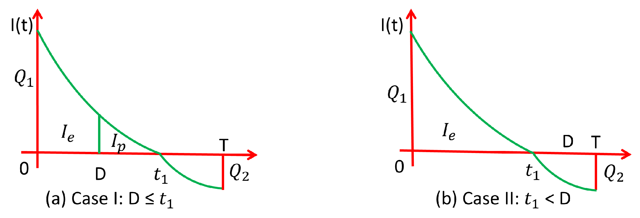
Figure 2.
Illustration of interlink and strategy of proposed inventory system
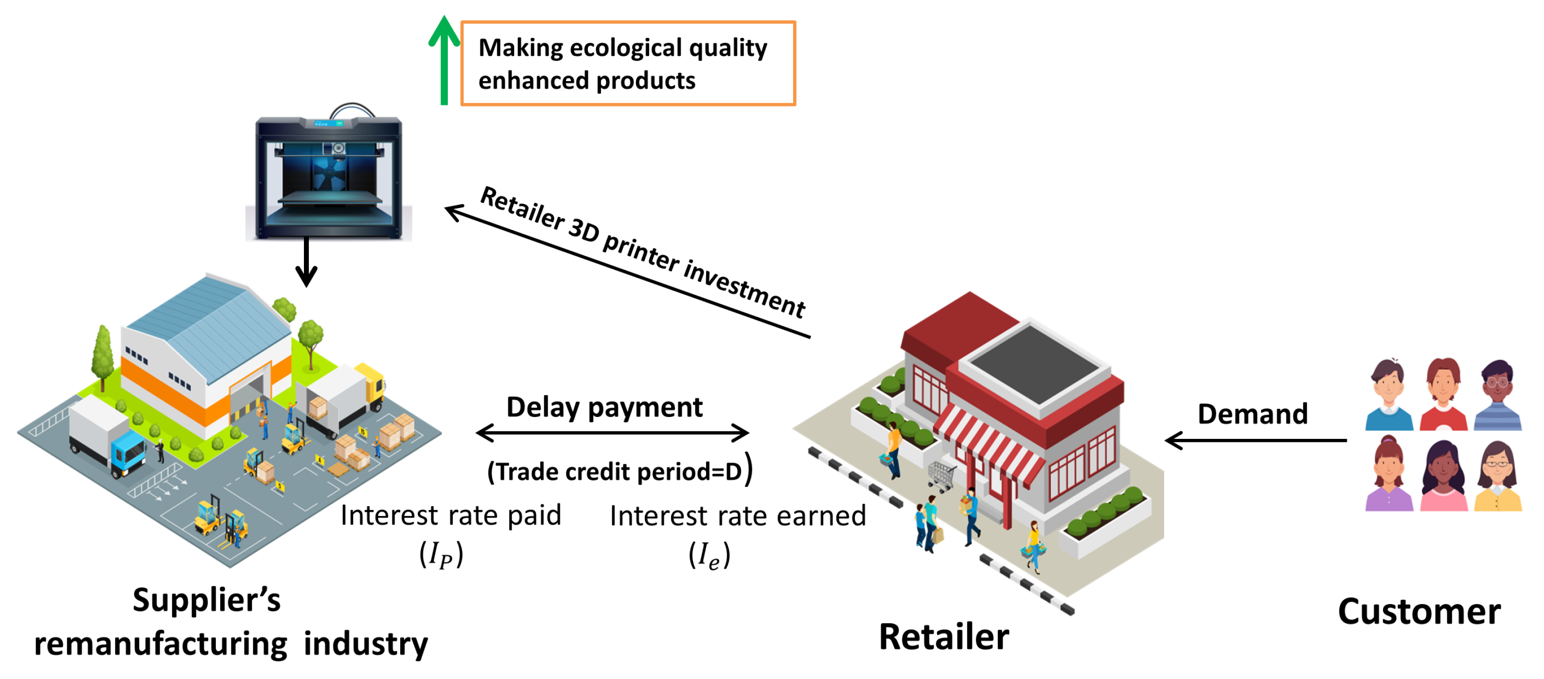
Figure 7.
Figure Figure 7(a) and Figure 7(b) illustrate the investment efficiency for with and without investment of AM technology for and , respectively.
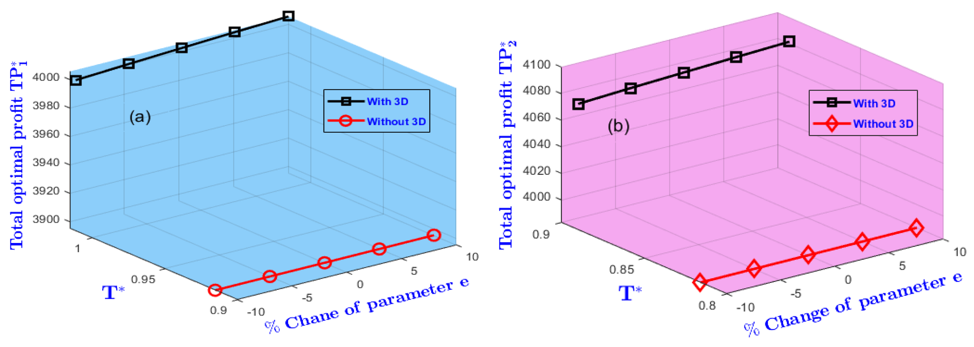
Figure 8.
Impact of the AM technology investment parameter comparing investment scenarios on AM technology for and by Fig.(a) and Fig.(b), respectively.
Figure 8.
Impact of the AM technology investment parameter comparing investment scenarios on AM technology for and by Fig.(a) and Fig.(b), respectively.
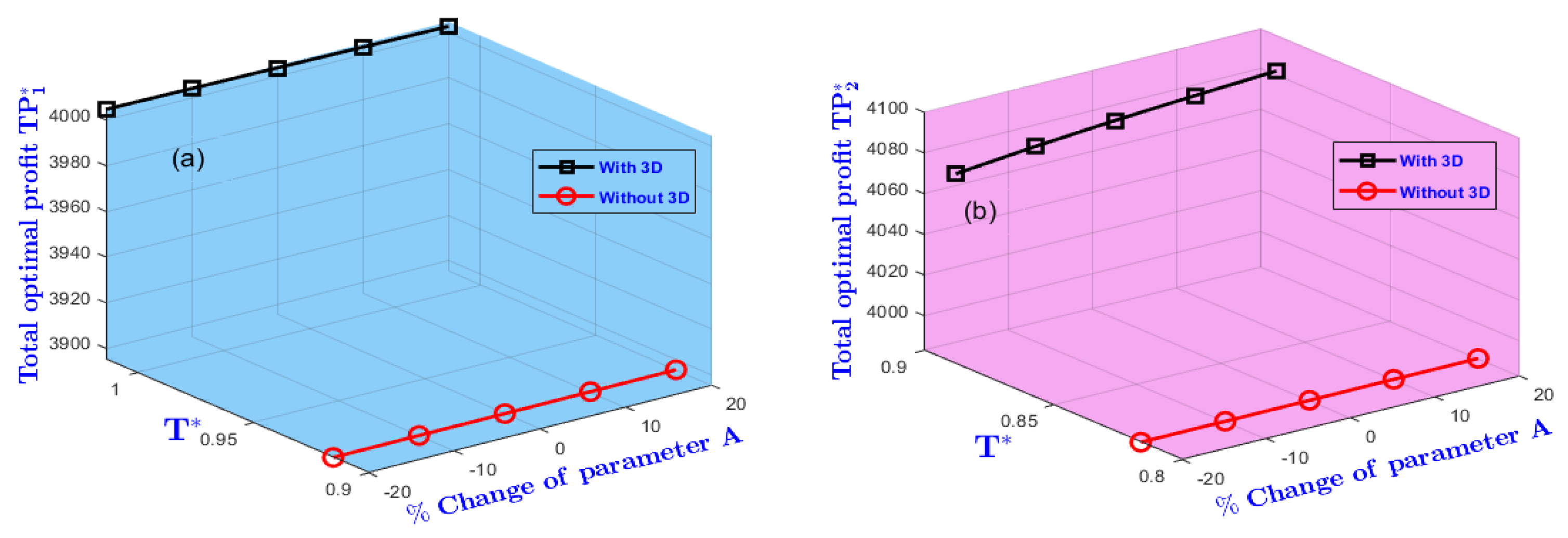
Figure 9.
Effect of reliability parameter for with and without AM technology investment for and illustrating by Fig.(a) and Fig.(b), respectively.
Figure 9.
Effect of reliability parameter for with and without AM technology investment for and illustrating by Fig.(a) and Fig.(b), respectively.
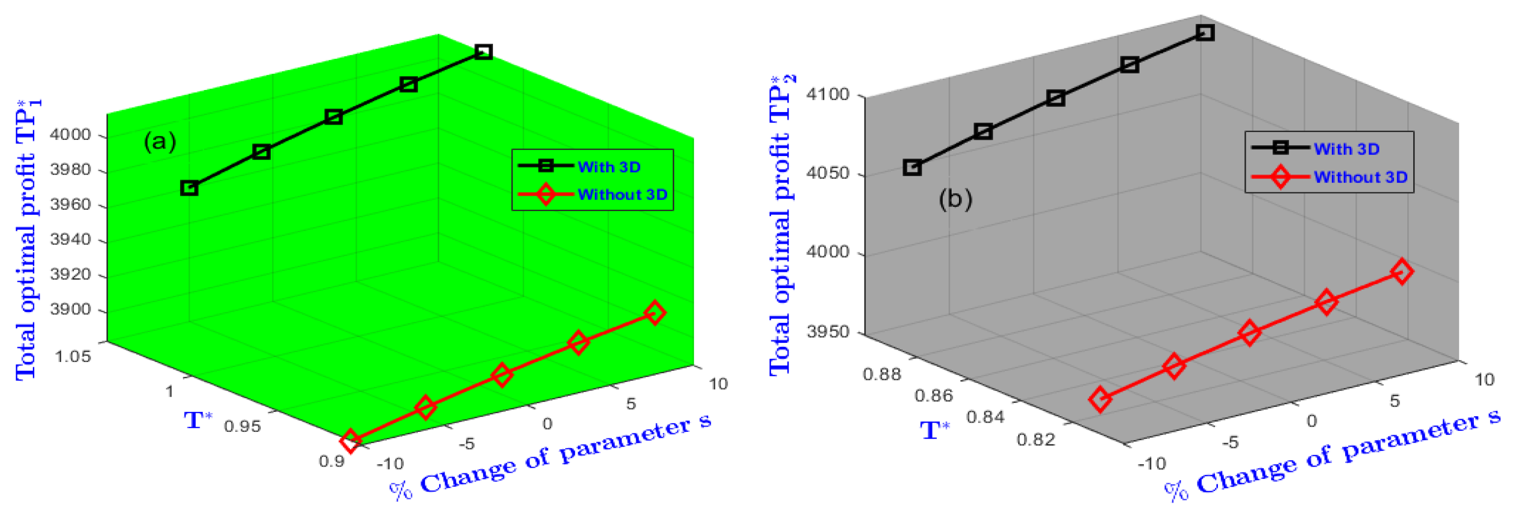
Table 2.
Optimum total profit associated with varying delay payment
| Delay of payments |
(year) | (year) | ||||
| 3 month (D=0.25) |
0.5883 | 0.9972 | 3995 | 0.4859 | 0.9134 | 3969 |
| 5 month (D=0.4167) |
0.6050 | 1.0040 | 4001 | 0.5198 | 0.9043 | 4022 |
| 7 month (D=0.5833) |
0.6229 | 1.0138 | 4004 | 0.5518 | 0.8913 | 4080 |
| 8 month (D=0.6667) |
0.6324 | 1.0199 | 4004 | 0.5672 | 0.8834 | 4110 |
| 9 month (D=0.75) |
0.6422 | 1.0265 | 4003 | 0.5821 | 0.8745 | 4142 |
Table 3.
Assessment of Additive manufacturing on optimal solution.
| Additive manufacturing | (year) | (year) | ||||
| With | 0.6229 | 1.0138 | 4004 | 0.5518 | 0.8913 | 4080 |
| Without | 0.5680 | 0.9154 | 3896 | 0.5518 | 0.8160 | 3983 |
Table 4.
Impact of cost parameters on variables and total costs via sensitivity analysis by evaluating % of change
Table 4.
Impact of cost parameters on variables and total costs via sensitivity analysis by evaluating % of change
| Cost | % change |
(year) |
% | % | % |
(year) | % | % | % |
||||
| -12 | 0.5808 | -9.34 | 0.9525 | -10.29 | 4065 | 2.60 | 0.5248 | -8.35 | 0.8319 | -11.37 | 4150 | 2.92 | |
| -10 | 0.5946 | -4.54 | 0.9630 | -5.01 | 4054 | 1.25 | 0.5295 | -4.04 | 0.8421 | -5.52 | 4138 | 1.42 | |
| 10 | 0.6500 | 4.35 | 1.0624 | 4.79 | 3956 | -1.20 | 0.5731 | 3.86 | 0.9381 | 5.25 | 4025 | -1.35 | |
| 12 | 0.6758 | 8.49 | 1.1089 | 9.38 | 3909 | -2.37 | 0.5934 | 7.54 | 0.9828 | 10.27 | 3973 | -2.62 | |
| -20 | 0.6422 | 3.10 | 0.9979 | -1.57 | 4389 | 9.62 | 0.5735 | 3.93 | 0.8972 | 0.66 | 4450 | 9.07 | |
| -10 | 0.6323 | 1.51 | 1.0055 | -0.82 | 4196 | 4.80 | 0.5621 | 1.87 | 0.8940 | 0.30 | 4265 | 4.53 | |
| 10 | 0.6142 | -1.40 | 1.0228 | 0.89 | 3811 | -4.82 | 0.5426 | -1.67 | 0.8890 | -0.26 | 3895 | -4.53 | |
| 20 | 0.6060 | -2.71 | 1.0324 | 1.83 | 3620 | -9.59 | 0.5343 | -3.17 | 0.8872 | -0.46 | 3710 | -9.07 | |
| -20 | 0.6363 | 2.15 | 1.0185 | 0.46 | 4009 | 0.12 | 0.5595 | 1.40 | 0.8933 | 0.22 | 4085 | 0.12 | |
| -10 | 0.6295 | 1.06 | 1.0161 | 0.23 | 4007 | 0.07 | 0.5556 | 0.69 | 0.8923 | 0.11 | 4082 | 0.05 | |
| 10 | 0.6165 | -1.03 | 1.0116 | -0.22 | 4001 | -0.07 | 0.5481 | -0.67 | 0.8903 | -0.11 | 4077 | -0.07 | |
| 20 | 0.6102 | -2.04 | 1.0094 | -0.43 | 3998 | -0.15 | 0.5444 | -1.34 | 0.8893 | -0.22 | 4075 | -0.12 | |
| -20 | 0.5781 | -7.91 | 1.0374 | 2.33 | 4023 | 0.47 | 0.5279 | -4.33 | 0.9163 | 2.80 | 4096 | 0.39 | |
| -10 | 0.6024 | -3.29 | 1.0246 | 1.07 | 4013 | 0.22 | 0.5407 | -2.01 | 0.9029 | 1.30 | 4087 | 0.17 | |
| 10 | 0.6407 | 2.86 | 1.0046 | -0.91 | 3996 | -0.20 | 0.5617 | 1.79 | 0.8810 | -1.16 | 4073 | -0.17 | |
| 20 | 0.6561 | 5.33 | 0.9965 | -1.71 | 3989 | -0.37 | 0.5705 | 3.39 | 0.8721 | -2.15 | 4067 | -0.32 | |
| -20 | 0.6371 | 2.28 | 1.0188 | 0.49 | 4010 | 0.15 | 0.5600 | 1.49 | 0.8935 | 0.25 | 4085 | 0.12 | |
| -10 | 0.6300 | 1.14 | 1.0163 | 0.25 | 4007 | 0.07 | 0.5559 | 0.74 | 0.8923 | 0.11 | 4083 | 0.07 | |
| 10 | 0.6161 | -1.09 | 1.0114 | -0.24 | 4001 | -0.07 | 0.5479 | -0.71 | 0.8902 | -0.12 | 4077 | -0.07 | |
| 20 | 0.6094 | -2.17 | 1.0091 | -0.46 | 3998 | -0.15 | 0.5439 | -1.43 | 0.8892 | -0.24 | 4075 | -0.12 |
Table 5.
Sensitivity analysis of parameters related to additive manufacturing technology on decision variables and objectives.
Table 5.
Sensitivity analysis of parameters related to additive manufacturing technology on decision variables and objectives.
| Parameter | % change |
(year) |
% | % | % |
(year) | % | % | % |
||||
| -20 | 0.6202 | -0.43 | 1.0089 | -0.48 | 4000 | -0.10 | 0.5501 | -0.31 | 0.8876 | -0.41 | 4076 | -0.10 | |
| A | -10 | 0.6217 | -0.19 | 1.0116 | -0.22 | 4002 | -0.05 | 0.5510 | -0.14 | 0.8896 | -0.19 | 4078 | -0.05 |
| 10 | 0.6240 | 0.18 | 1.0158 | 0.20 | 4005 | 0.02 | 0.5525 | 0.13 | 0.8927 | 0.16 | 4081 | 0.02 | |
| 20 | 0.6250 | 0.34 | 1.0174 | 0.36 | 4006 | 0.05 | 0.5531 | 0.24 | 0.8940 | 0.30 | 4082 | 0.05 | |
| -20 | 0.5815 | -6.65 | 0.9394 | -7.34 | 3920 | -2.10 | 0.5248 | -4.89 | 0.8346 | -6.36 | 4005 | -1.84 | |
| y | -10 | 0.6011 | -3.50 | 0.9746 | -3.87 | 3961 | -1.07 | 0.5377 | -2.56 | 0.8616 | -3.33 | 4042 | -0.93 |
| 10 | 0.6475 | 3.95 | 1.0579 | 4.35 | 40481 | 1.10 | 0.5675 | 2.85 | 0.9240 | 3.67 | 4119 | 0.96 | |
| 20 | 0.6751 | 8.38 | 1.1078 | 9.27 | 4094 | 2.25 | 0.5848 | 5.98 | 0.9604 | 7.75 | 4160 | 1.96 | |
| -20 | 0.6106 | -1.97 | 0.9917 | -2.18 | 3980 | -0.60 | 0.5439 | -1.43 | 0.8746 | -1.87 | 4059 | -0.51 | |
| -10 | 0.6167 | -1.00 | 1.0026 | -1.10 | 3992 | -0.30 | 0.5478 | -0.72 | 0.8829 | -0.94 | 4069 | -0.27 | |
| 10 | 0.6294 | 1.04 | 1.0254 | 1.14 | 4016 | 0.30 | 0.5560 | 0.76 | 0.8999 | 0.96 | 4091 | 0.27 | |
| 20 | 0.6360 | 2.10 | 1.0374 | 2.33 | 4028 | 0.60 | 0.5602 | 1.52 | 0.9088 | 1.96 | 4101 | 0.51 | |
| -10 | 0.6218 | -0.18 | 1.0116 | -0.22 | 4001 | -0.07 | 0.5511 | -0.13 | 0.8896 | -0.19 | 4078 | -0.05 | |
| e | -5 | 0.6224 | -0.08 | 1.0127 | -0.11 | 4003 | -0.02 | 0.5514 | 0.07 | 0.8904 | 0.10 | 4082 | -0.02 |
| 5 | 0.6235 | 0.10 | 1.0148 | 0.10 | 4005 | 0.02 | 0.5522 | 0.07 | 0.8920 | 0.08 | 4081 | 0.02 | |
| 10 | 0.6240 | 0.18 | 1.0517 | 0.19 | 4006 | 0.05 | 0.5525 | 0.13 | 0.8927 | 0.16 | 4082 | 0.05 |
Table 6.
Sensitivity analysis of the different parameters incorporating AM investment by evaluating % of change of decision variables and objectives.
Table 6.
Sensitivity analysis of the different parameters incorporating AM investment by evaluating % of change of decision variables and objectives.
| Parameter | % change | (year) | % | % | % | (year) | % | % | % | ||||
| -20 | 0.6486 | 4.13 | 1.0599 | 4.55 | 3045 | -23.95 | 0.5770 | 4.57 | 0.9495 | 6.63 | 3100 | -24.02 | |
| a | -10 | 0.6353 | 1.99 | 1.0360 | 2.19 | 3524 | -11.99 | 0.5640 | 2.21 | 0.9192 | 3.13 | 3589 | -12.03 |
| 10 | 0.6115 | -1.83 | 0.9933 | -2.02 | 4484 | 11.99 | 0.5406 | -2.03 | 0.8656 | -2.88 | 4571 | 12.03 | |
| 20 | 0.6009 | -3.53 | 0.9742 | -3.91 | 4964 | 23.98 | 0.5301 | -3.93 | 0.8418 | -5.55 | 5064 | 24.12 | |
| -5 | 0.6469 | 3.85 | 1.0569 | 4.25 | 4047 | 1.07 | 0.5671 | 2.77 | 0.9233 | 3.59 | 4119 | 0.96 | |
| b | -3 | 0.6370 | 2.26 | 1.0390 | 2.49 | 4029 | 0.62 | 0.5609 | 1.65 | 0.9101 | 2.11 | 4103 | 0.56 |
| 10 | 0.5822 | -6.53 | 0.9408 | -7.20 | 3922 | -2.05 | 0.5252 | -4.82 | 0.8357 | -6.24 | 2006 | -1.81 | |
| 20 | 0.5489 | -11.88 | 0.8811 | -13.09 | 3845 | -3.97 | 0.5029 | -8.86 | 0.7891 | -11.47 | 3937 | -3.50 | |
| -20 | 0.6107 | -1.96 | 0.9917 | -2.18 | 3980 | -0.60 | 0.5439 | -1.43 | 0.8746 | -1.87 | 4059 | -0.51 | |
| x | -10 | 0.6167 | -1.00 | 1.0026 | -1.10 | 3992 | -0.30 | 0.5478 | -0.72 | 0.8828 | -0.95 | 4069 | -0.27 |
| 10 | 0.6294 | 1.04 | 1.0254 | 2.33 | 4016 | 0.30 | 0.5560 | 0.76 | 0.8999 | 0.96 | 4091 | 0.27 | |
| 20 | 0.6361 | 2.12 | 1.0374 | 2.33 | 4028 | 0.60 | 0.5602 | 1.52 | 0.9088 | 1.06 | 4101 | 0.51 | |
| -5 | 0.6590 | 5.80 | 1.0787 | 6.40 | 3716 | -7.19 | 0.5744 | 4.108 | 0.9392 | 5.37 | 3786 | -7.21 | |
| p | -3 | 0.6443 | 3.44 | 1.0522 | 3.79 | 3832 | -4.30 | 0.5652 | 2.43 | 0.9197 | 3.19 | 3904 | -4.31 |
| 10 | 0.5588 | -10.29 | 0.8990 | -20.81 | 4571 | 14.16 | 0.5105 | -7.48 | 0.8032 | -9.88 | 4666 | 14.24 | |
| 20 | 0.5049 | -18.94 | 0.8028 | -20.81 | 5132 | 28.17 | 0.4745 | -14.01 | 0.7264 | -18.50 | 5235 | 28.31 | |
| -10 | 0.6153 | -1.22 | 1.0002 | -1.16 | 3989 | -0.37 | 0.5470 | -6.87 | 0.8810 | -1.16 | 4067 | -0.32 | |
| s | -5 | 0.6193 | -0.58 | 1.0074 | -0.63 | 3997 | -0.17 | 0.5495 | -0.42 | 0.8864 | -0.55 | 4074 | -0.15 |
| 5 | 0.6262 | 0.53 | 1.0196 | 0.57 | 4010 | 0.15 | 1.5539 | 0.38 | 0.8955 | 0.47 | 4085 | 0.12 | |
| 10 | 0.6291 | 1 | 1.0248 | 1.09 | 4015 | 0.27 | 0.5558 | 0.72 | 0.8994 | 0.91 | 4090 | 0.25 |
Disclaimer/Publisher’s Note: The statements, opinions and data contained in all publications are solely those of the individual author(s) and contributor(s) and not of MDPI and/or the editor(s). MDPI and/or the editor(s) disclaim responsibility for any injury to people or property resulting from any ideas, methods, instructions or products referred to in the content. |
© 2025 by the authors. Licensee MDPI, Basel, Switzerland. This article is an open access article distributed under the terms and conditions of the Creative Commons Attribution (CC BY) license (http://creativecommons.org/licenses/by/4.0/).
Copyright: This open access article is published under a Creative Commons CC BY 4.0 license, which permit the free download, distribution, and reuse, provided that the author and preprint are cited in any reuse.


