
Submitted:
09 May 2023
Posted:
11 May 2023
You are already at the latest version
Abstract
The mathematical modelling of reverse logistics inventory systems ignores that returned items may arrive out of sequence, i.e. with different number of remanufacturing times. Moreover, such modelling assumes that the retuned items may retain the same quality upon recovery regardless of how many times they have been previously remanufactured. This paper develops a new mathematical expression of the percentage of retuned items that can be remanufactured a finite number of times. The proposed expression is modelled as a function of the expected number of times an item can be remanufactured on its life cycle and the number of times an item can be technologically (or optimally) remanufactured based on its quality upon recovery. The model developed in this paper considers joint production and remanufacturing options. The return rate is a varying demand dependent rate, which is a decision variable with demand, product deterioration, manufacturing and remanufacturing rates being arbitrary functions of time. The model considers the initial inventory of returned items in the mathematical formulation, which enables decision makers to adjust all functions and input parameters for subsequent cycles. Illustrative examples indicate that dependent purchasing price of recovery items and the incorporation of remanufacturing investment cost significantly impact on the optimal remanufacturing policy.
Keywords:
reverse logistics
; number of remanufacturing times
; first remanufacturing cycle
; time-varying parameters
; demand dependent return rate
1. Introduction
Reverse logistics emerges as an opportunity beyond
traditional logistics role with the main purpose being product returns from end
customers for recapturing value or proper disposal (Fleischmann et al., 1997).
Further, reverse logistics has been implemented to address economic drivers,
government pressure/legislation, social interests and environmental
consciousness. The goal of reverse logistic is to effectively manage and
control the flow of products returned from end customers to extend their
useable lives, reduce solid waste disposal and conserve natural resource
consumption (De Brito and Dekker, 2004; Rogers and Tibben-Lembke, 2001). The
importance of reverse logistics may vary from one industry to another due to
relevant costs and the dynamic nature of production and remanufacturing
processes of the products. The reverse logistics process is a merroir image of
the traditional forward supply chain one. It comprises activities such as the
collection of returned items from end users, their inspection, their
processing, their disassembly and finally their distribution for recovery
purposes (Bei and Linyan, 2005; De Brito and Dekker, 2004). Whereas a
closed-loop supply chain is categorised by the combination of forward and
reverse supply chain activities (Bei and Linyan, 2005; Guide et al., 2003).
Supply chain management in reverse logistics has
growing attention in recent years. Moreover, due to global competitiveness,
there has been more focus among large companies to adopt joint production and
remanufacturing options in their businesses (Andrade et al., 2013; Rubio and
Jiménez-Parra, 2017). For example, in Germany, about 10% of engines and starter
engines are remanufactured (Bras 2007). In this regard, the remanufactured
products save 80% of raw materials, require 33% of the labour force, consume 50%
of the energy and up to 50%–70% less cost when compared with the newly
manufactured products (Cao et al. 2020; Liu et al. 2020; Van Nguyen et al.
2020; Wang et al. 2020). Several companies including BMW and Volkswagen focus
on accelerating the upgrading process of older cars and offer fully warrantied
service for remanufactured engines and other parts (Flapper et al. 2005; Liu et
al. 2020). Therefore, reverse logistics can enhance productivity, reduce costs,
improve profitability, meet total product demand and avoid the tarnished
reputation associated with customer loyalty (Fleischmann, 2001).
Beyond the economic benefits, there exists a
plethora of factors such as social and environmental consciousness and
government legislation that may force manufacturers to include such product
recovery systems in their businesses (Montabon et al., 2016).
2. Literature review
The first inventory model with returned items was
conducted by Schrady (1967). He developed a deterministic Economic Order
Quantity (EOQ) model for repaired items with the assumption that manufacturing,
and recovery (repair) rates are instantaneous with no disposal cost. Nahmias
and Rivera (1979) generalised the model of Schrady (1967) for the case of
finite repair rate. Richter (1996a, 1996b, 1997), Richter and Dobos (1999) and
Dobos and Richter (2000) carried out several investigations into the EOQ repair
and waste disposal model, where the return rate is considered as a decision
variable. Richter (1996a, 1996b) considered a modified version of the model of
Schrady (1967) by investigating multiple repair and production cycles within a
time interval. Dobos and Richter (2003) investigated a manufacturing/recycling
system for non-instantaneous manufacturing and recycling rates.
Richter (1997) examined the optimal inventory
holding policy when the waste disposal (return) rate is a decision variable.
The result of his paper is that the optimal policy is governed by a pure
(bang–bang) strategy of either no repair (total waste disposal) or no waste
disposal (total repair). Dobos and Richter (2004) generalised their previous
work (Dobos and Richter, 2003) for multiple repair and production cycles.
Results indicated that a pure strategy is optimal compared to a mixed strategy.
Dobos and Richter (2006) assumed that some collected returned items are not
always suitable for further recycling. There are numerous studies that relax
different assumptions made so far. Examples of these works are cited in (Bazan
et al. 2016).
El Saadany and Jaber (2010) considered the
collection rate of returned items to be dependent on the purchasing price and
the use proportion of these returns. Their results showed that a mixed
(production + remanufacturing) strategy is optimal, when compared to a pure
strategy as suggested by Dobos and Richter (2003, 2004). Alamri (2011)
generalised the first model of El Saadany and Jaber (2010) and verified the
examples given in Dobos and Richter (2003, 2004) and El Saadany and Jaber
(2010). He showed that a mixed strategy dominates a pure strategy.
El Saadany and Jaber (2008) pointed out that
previous studies assumed an infinite planning horizon and did not account for
the first cycle as there are no returned items to be remanufactured. They rectified
a minor error in the work of Richter (1996a, 1996b) and, consequently, their
model produces a lower cost because of the residual inventory assumed in
Richter’s model. Kozlovskaya et al. (2017) generalised the work of El Saadany
and Jaber (2008) and corrected the optimal solution for their model. They
showed that the optimal policy depends on the disposal rate. Although El
Saadany and Jaber (2008) have provided a closed form formula for the first
cycle, their mathematical formulation as well as the other studies in the
literature are alike. Alamri (2021) discussed this issue in detail and
addressed this limitation by incorporating the initial inventory of returned
items in the mathematical formulation. He showed that the optimal policy
implies that the cumulative inventory for returned items vary for each cycle
before the system plateaus. This is a key consideration that allows the decision
maker to change the values of the input parameters for subsequent cycles.
In this section, we have cited research that are
directly relevant to this paper. For more details about inventory models
related to reverse logistics systems, see (Govindan et al., 2015 Modak. et al.
2023).
3. Research background and contribution
In this section, we address some issues that are
related to the number of times a product can be remanufactured as advocated in
El Saadany et al. (2013), followed by some discussion that elaborates on our
research contributions. Meanwhile, the work of Alamri (2021) constitutes the
base model of this research.
3.1. Theoretical background and motivation
El Saadany et al. (2013) developed a mathematical
expression that indicates the number of times a product can be remanufactured.
They attempted to relax the general assumption that a product can be remanufactured
for an indefinite number of times. They assumed that an item can be recovered
for a limited number of times. When the system plateaus, then
for any , a fraction of a constant demand rate is remanufactured and is produced, where and is the proportion of used items returned for
remanufacturing when an item is recovered an indefinite number of times. It is
worth noting here that the mathematical expression used to derive focused on the returns of what was produced on
previous period and ignored the rest of cumulative produced quantities that
have been left or previously being remanufactured. Interested readers are
referred to Table 1 in El Saadany et al.
(2013). They stated that as , , which is what has been suggested in the existing
literature. For a pure production case, i.e., , , though a pure production strategy implies that , i.e., there are no items returned for recovery
purposes. Moreover, the mathematical expression used to derive assumes that no waste disposal (total repair) of
the proportion upon recovery. Then, they
modified the work of Richter (1997) and Teunter (2001) by replacing with in Richter’s and Teunter’s models.

Table 1.
The actual quality level of an item that recovers number of times when .
| 1 | 2 | 3 | 4 | 5 | 6 | 7 | 8 |
|---|---|---|---|---|---|---|---|
| 0.368 | 0.607 | 0.717 | 0.779 | 0.819 | 0.846 | 0.867 | 0.882 |
| 0.368 | 0.513 | 0.607 | 0.670 | 0.717 | 0.751 | 0.779 | |
| 0.368 | 0.472 | 0.549 | 0.607 | 0.651 | 0.687 | ||
| 0.368 | 0.449 | 0.513 | 0.565 | 0.607 | |||
| 0.368 | 0.435 | 0.490 | 0.535 | ||||
| 0.368 | 0.424 | 0.472 | |||||
| 0.368 | 0.417 | ||||||
| 0.368 |
In their model, the produced quantity is also disposed outside
the system (e.g., Bazan et al., 2015) since they have defined as the disposal rate,
where . Moreover, the role of in their model is somewhat ambiguous. Therefore,
we can distinguish three cases: (1) As can be seen from Figure 1 in El Saadany et al. (2013),
entering the repairable
stock from which is remanufactured and is disposed. This implies
that the return rate is , however, this contradicts what the existing literature suggests, i.e., the return rate is less than demand rate; (2) , which is a function of , and therefore, the value of is used to compute . In their examples, is defined as the collection of used items and is the effective proportion. In this case (case
2), one can deduce that enters the repairable
stock from which is remanufactured and is disposed. However, represents the proportion of used items returned
for remanufacturing when an item is recovered an indefinite number of times and
only of is remanufactured; (3) The return rate is , which enters the repairable stock and flows in
the serviceable stock to be remanufactured with no waste disposal (total
repair). That is, the purpose of , which represents (the proportion of used items
returned for remanufacturing when an item is recovered an indefinite number of
times) is to compute . In this case (case 3), the system should collect instead of , which is reflected in their modified version of
the work of Richter (1997) and Teunter (2001). Hence, we can conclude that in
all cases, is used to compute , with case 2 being the most appropriate scenario.
However, in all these cases, has no relation with an item
being recovered for a limited number of times. In fact, is an arbitrary integer value, which implanted in to minimise the total cost. Therefore, considering
a fraction of the return rate that
meets the acceptance quality level to be remanufactured and is disposed outside the system is more practicable
(Dobos and Richter, 2004; El Saadany and Jaber, 2010, Alamri, 2011; Alamri, 2021).
The difference between and represents about 50% when and (see Figure 1).
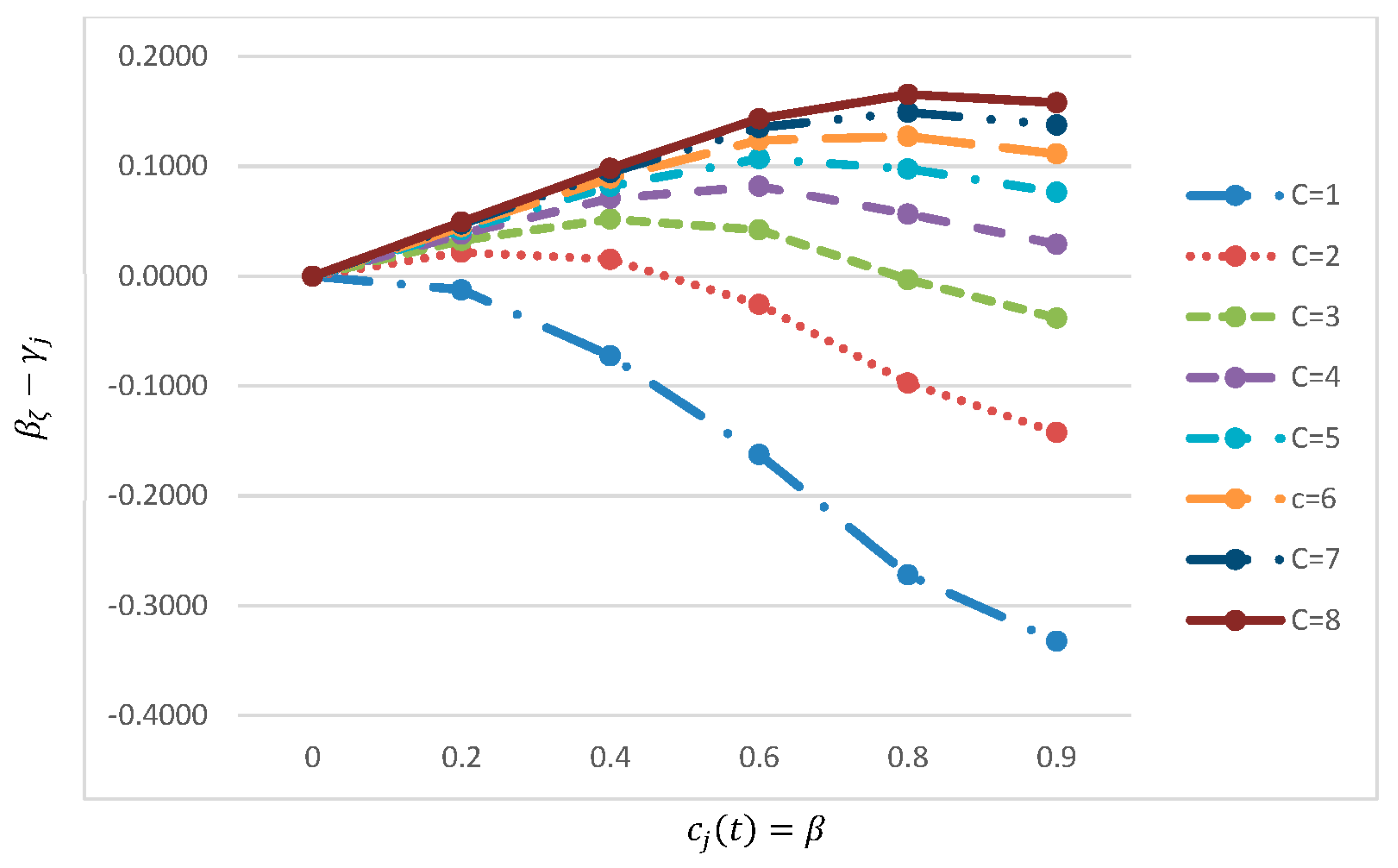
Moreover, for a fixed value of , this difference decreases with (see Figure 2
in El Saadany et al. (2013) page 600 and Figure
1 in this paper). This seems logical in their expression, since as , because they assumed that all returned items have been remanufactured number of times. On the
contrary, however, this difference should increase as a returned item with a
greater number of remanufacturing times recovers with inferior quality.
Furthermore, implementing as suggested by El Saadany et al. (2013) would
result in a large disposal quantity especially for products that are associated
with relatively small number of recovery times since increases with (see Figure 2).
Finally, incorporating such in the mathematical formulation entails that all
returned items have been remanufactured number of times. However, fact remains that returned items may arrive out of sequence, i.e., with different number of remanufacturing times assuming also that previous number of remanufacturing times is labelled. It is true to say that considering such classification of returned items in the mathematical expression is not an easy task, however, this limitation will be discussed in the next section.
Figure 1.
The behaviour of (a reproduction of as in El Saadany et al. (2013)).
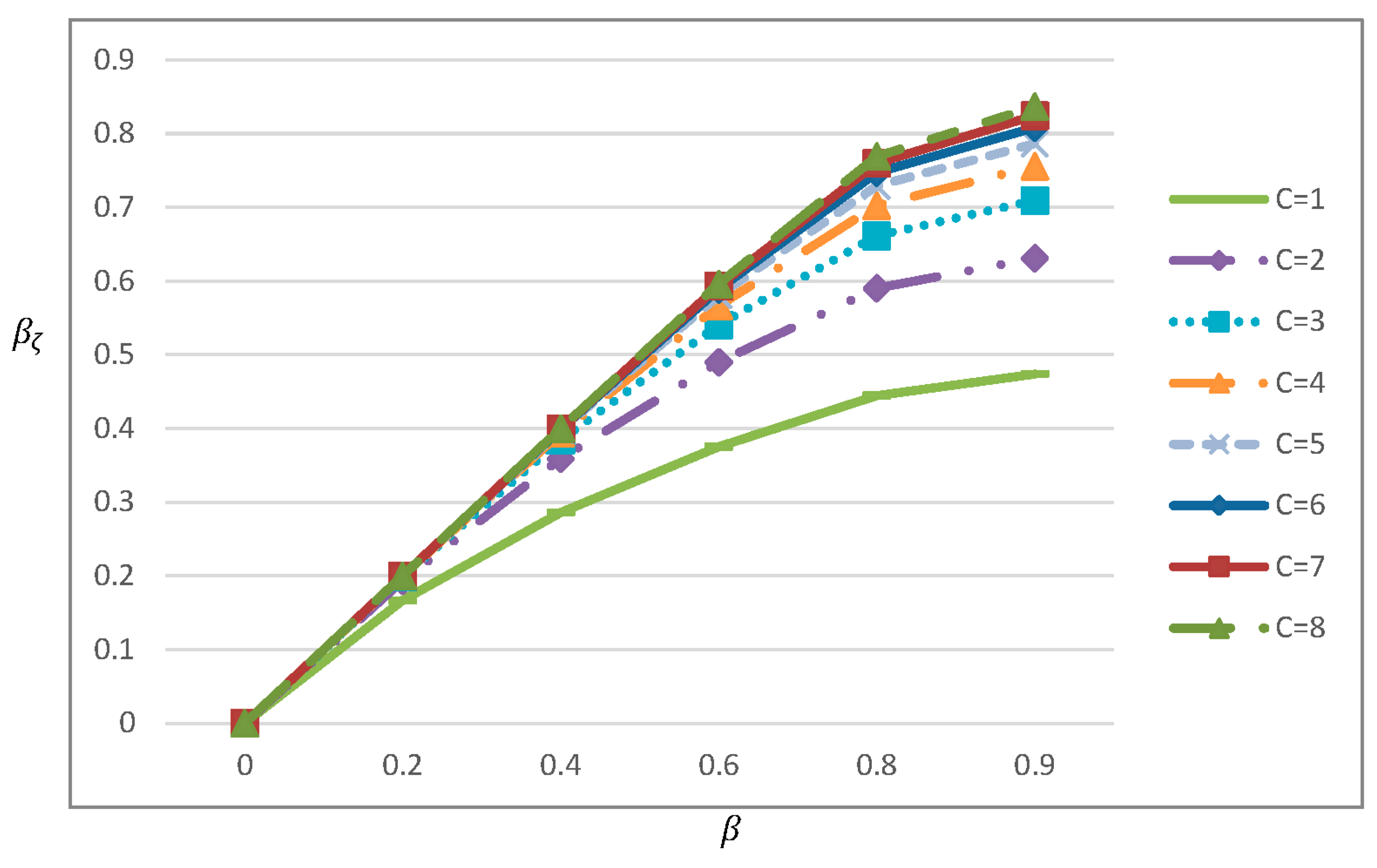
Figure 2.
The difference between and .
3.2. Mathematical formulation of the recovery times
The comprehensive discussion in the previous section is necessary to position our study in the existing literature and highlights its research contribution. This paper aims to enhance this line of research by developing a new mathematical expression that models the percentage of returns as a function of the number of times an item is recovered, the corresponding quality for the recovery item and the expected number of times an item can be remanufactured on its life cycle. In this paper, we assume that returned items are collected at a rate of (decision variable) where denotes the cycle index. Note that a pure
production strategy occurs when .
Only a fraction of these retuned items can be remanufactured.
Namely, , where denotes the quality level of an item that has been
recovered number of times. We assume
that , where , i.e., it refers to the quality of a newly
manufactured item. In this paper, refers to the maximum number of times an item can
be technologically (or optimally) remanufactured and denotes the expected
number of times an item can be remanufactured on its life cycle. Note that decreases as increseas and it attains a minimum value as in this case, (Table 1).
Accordingly, a recovery item with a quality less than the minimum acceptance
quality level is considered defective and
incurs a disposal cost. Note that and , i.e., is a monotonically
decreasing function over and, as . The same arguments hold true for . This implies that is modelled as a function of the expected number
of times an item can be remanufactured on its life cycle and the number of
times an item can be technologically remanufactured based on its quality upon
recovery. Moreover, and are free from any judgmental
measurements.
In real life settings, returned items may recover
out of sequence. This can be attributed to random number of times these items
have been remanufactured. Let us define the returned amount for cycle as , where this amount undergoes a 100 per cent
inspection. Assuming an automated remanufacturing system, the observation of seems realistic since all returned items are
inspected. Therefore, returned items that are subjected to a 100 per cent
screening upon recovery to the repairable stock would imply that . That is, is the collected used/returned items with is the number of times
these items have been previously remanufactured. Here, denotes returned items that have not yet being
remanufactured, and refers to defective
(disposed) returned items that have been remanufactured number of times or items
that do not meet the minimum acceptance quality level, .
It is worth noting here, that the above-mentioned
classification seams realistic because the system can deal with items based on
such classification upon recovery. Therefore, as the number of times an item
can be recovered increases, its corresponding use proportion decreases. This
finding, however, contradicts that of El Saadany et al. (2013). To justify
this, suppose that among the returned quantity that can be remanufactured say,
5 times there exists a sub-quantity arrived at the repairable stock with its
first-time recovery. In this case, implementing for this sub-quantity would result in disposing an
equal fraction as that of items with a greater recover time, though these items
have not yet been remanufactured. Table 2
depicts the corresponding use proportion where . For instance, if a quantity of returned items
that can be remanufactured say, 5 times, then each sub-quantity is associated
with its corresponding accepted fraction, i.e., . That is, represents the use proportion of the sub-quantity
of the retuned items that can be remanufactured for its remanufacturing time. However, considering the
above-mentioned classification in the mathematical formulation emerges as a
challenge that affects the tractability problems in modelling. Therefore, to
tackle this issue, we suggest that which constitutes an approximation of the average
fraction (cumulative average up to ) that can be remanufactured in cycle (Figure 3).
Figure 3.
The behaviour of that flows to be remanufactured in cycle .
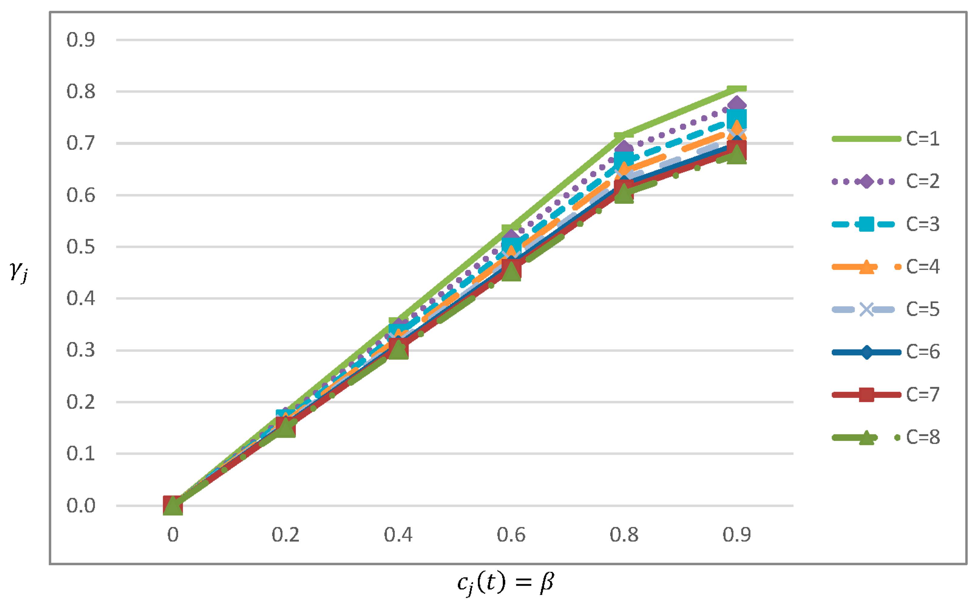
Table 2.
The actual proportion of returned items that can be remanufactured number of times when .
| 1 | 2 | 3 | 4 | 5 | 6 | 7 | 8 |
|---|---|---|---|---|---|---|---|
| 0.692 | 0.738 | 0.788 | 0.823 | 0.849 | 0.868 | 0.884 | 0.896 |
| 0.692 | 0.710 | 0.738 | 0.765 | 0.788 | 0.807 | 0.823 | |
| 0.692 | 0.702 | 0.719 | 0.738 | 0.756 | 0.773 | ||
| 0.692 | 0.698 | 0.710 | 0.724 | 0.738 | |||
| 0.692 | 0.696 | 0.705 | 0.716 | ||||
| 0.692 | 0.695 | 0.702 | |||||
| 0.692 | 0.694 | ||||||
| 0.692 |
As can be seen from Table 2, assuming to be remanufactured in
cycle implies that the proportion is disposed outside the system. Conversely,
, i.e., considers the cumulative average up to time of returned items (Table
4). This is a key consideration because it governs the behaviour of
returned items and ensures reducing the disposal of unnecessary amount. In
addition, returned items are coupled with distinct purchasing price , where denotes unit purchasing price for new items.
Table 3.
The average fraction (cumulative average up to ) of the quality level of items that recover for their time when .
Table 3.
The average fraction (cumulative average up to ) of the quality level of items that recover for their time when .
| 1 | 2 | 3 | 4 | 5 | 6 | 7 | 8 |
|---|---|---|---|---|---|---|---|
| 0.368 | 0.607 | 0.717 | 0.779 | 0.819 | 0.846 | 0.867 | 0.882 |
| 0.487 | 0.615 | 0.693 | 0.745 | 0.782 | 0.809 | 0.831 | |
| 0.533 | 0.619 | 0.679 | 0.723 | 0.757 | 0.783 | ||
| 0.556 | 0.622 | 0.671 | 0.709 | 0.739 | |||
| 0.571 | 0.624 | 0.665 | 0.698 | ||||
| 0.581 | 0.625 | 0.660 | |||||
| 0.588 | 0.626 | ||||||
| 0.593 |
Table 4.
The average fraction (cumulative average up to ) of returned items that can be remanufactured for their time when .
Table 4.
The average fraction (cumulative average up to ) of returned items that can be remanufactured for their time when .
| 1 | 2 | 3 | 4 | 5 | 6 | 7 | 8 |
|---|---|---|---|---|---|---|---|
| 0.692 | 0.738 | 0.788 | 0.823 | 0.849 | 0.868 | 0.884 | 0.896 |
| 0.715 | 0.749 | 0.781 | 0.807 | 0.828 | 0.845 | 0.859 | |
| 0.730 | 0.754 | 0.778 | 0.798 | 0.816 | 0.830 | ||
| 0.739 | 0.758 | 0.776 | 0.793 | 0.807 | |||
| 0.745 | 0.760 | 0.775 | 0.789 | ||||
| 0.749 | 0.762 | 0.775 | |||||
| 0.752 | 0.763 | ||||||
| 0.754 |
3.3. Contribution and organisation of the paper
This paper develops a new mathematical expression that specifies the number of times a product can be remanufactured. In particular, the proposed expression is modelled as a function of the expected number of times an item can be remanufactured on its life cycle and the number of times an item can be technologically (or optimally) remanufactured based on its quality upon recovery.
In this paper, we present a general reverse logistics inventory model with a single manufacturing cycle and a single remanufacturing cycle. Demand, deterioration, manufacturing, remanufacturing and return rates are arbitrary functions of time. Therefore, a diverse range of time-varying forms can be disseminated from the general model. The mathematical formulation consists of serviceable and reparable stocks. The serviceable stock is for new and remanufactured items and the reparable stock is for collecting returned items to be remanufactured in the serviceable stock as good as new. Therefore, different holding costs and deterioration rates are considered for manufactured, remanufactured and returned items (e.g., Alamri, 2011; Alamri et al., 2016; Jaber and El Saadany, 2009; Teunter, 2001).
Only a proportion of the returned items that specifies the number of times a product can be remanufactured flows in the serviceable stock. In the first remanufacturing cycle, the initial inventory of retuned items is zero since there are no returned items to be remanufactured. Therefore, the accumulated amount of returned items (during the time gap of non-production and non-remanufacturing processes) represents the initial inventory of returns for the second cycle. This amount, indeed, should differ from that accumulated for subsequent cycles. This is key in our formulation, and therefore, ensures that all optimal values vary for each cycle before the system plateaus. The proposed model accounts for setup changeover costs when switching from manufacturing phase to remanufacturing phase. The proposed model also considers an investment cost associated with the number of times a product is recovered. We assume that returned, manufactured and remanufactured items deteriorate while they are effectively in stock. The return rate of the returned items is a decision variable, which is a function of the demand rate. The purchasing price of returned items is a function of the purchasing price of new items and the quality of items upon recovery. All functions and input parameters can be adjusted for subsequent cycles.
The remainder of the paper is organised as follows: In Section 4, we present our joint manufacturing and remanufacturing model and the solution procedure. Illustrative examples, and special cases are offered in Section 5. Managerial insights and concluding remarks are provided in Section 6 and Section 7 respectively.
4. Mathematical formulation of the general model
4.1. Assumptions and notations
Our model is developed under the following notations:
The cycle index;
is for
manufactured items,
is for
remanufactured items and
is for returned items;
The inventory level at
time
;
The
manufactured rate per unit time for new items;
The remanufactured rate per unit time for returned items;
The demand rate per unit
time;
The return rate
per unit time for returned items (decision variable), where
and
;
The
deterioration rate per unit time;
The deteriorated
quantity for cycle ;
The manufactured
quantity for cycle ;
The remanufactured
quantity for cycle ;
The returned quantity for cycle ;
The accumulated quantity
of returned items (during the time gap of non-production and
non-remanufacturing processes);
The maximum number of
times an item can be remanufactured;
The expected number of
times an item can be remanufactured on its life cycle, where
;
The actual
quality level of an item that has been
recovered
number of times
in cycle
, where
(
Table
1
);
The average fraction
(cumulative average up to
) of the quality level of items that have
been
recovered
for their
time
in cycle
, where
(
Table
3
);
The actual proportion of
returned items that can be remanufactured in cycle
, where
(
Table 2
);
The average fraction
(cumulative average up to
) of returned items that can be
remanufactured
for
their
time
in cycle
, where
(
Table 4
);
The unit purchasing cost for
new items;
The unit
purchasing price for retuned items in cycle
, where
;
The
remanufacturing investment cost in the design process of
an
item
to, technologically, be able to remanufacture it
number of times
;
The
remanufacturing investment cost in cycle
in the design process of
an
item
to, technologically, be able to remanufacture it
number of times,
where
;
The unit manufacturing cost;
The unit remanufacturing
cost;
The unit screening cost;
The unit disposal cost for
deteriorated and scrap items;
The holding cost per unit per
unit time;
The set-up/order cost per
cycle;
The switching cost from remanufacturing
phase to manufacturing phase;
The switching cost from manufacturing
phase to remanufacturing phase;
Below is a list of all assumptions used in the paper:
- Returned items are collected throughout the time interval at a rate .
- Only a proportion of the returned items can be remanufactured and the amount is disposed as waste outside the system.
- New items are manufactured at a rate and the accepted returned items are remanufactured at a rate as good as new.
- The demand rate is satisfied from produced and remanufactured items.
- Items deteriorate at a rate while they are effectively in stock, and there is no repair or replacement of deteriorated items.
- The demand, product deterioration, manufacturing, and remanufacturing rates are arbitrary functions of time.
- The return rate is a varying demand dependent rate, which is a decision variable.
- The values of all functions and input parameters can be adjusted for subsequent cycles.
- Shortages are not allowed, i.e., we require that
4.2. The general model
In our model, demand in the first cycle is satisfies from production only (see Figure 5), as the inventory of returned items in the first cycle is zero (there are no returned items to be remanufactured). The process is repeated until inventory of product returns can be technologically attainable. Then, at the beginning of each cycle, the system starts the production prosses until
time , by which point in time units have been produced and
stored in the serviceable stock. At time , the inventory level of new items becomes zero and
units have deteriorated,
which refers to the difference between the satisfied demand during production
cycle and units that have been
manufactured in cycle. The remanufacturing process starts at time until time , by which point in time the remanufactured
quantity units have been
accumulated and stored in the serviceable stock. The returned items are
collected throughout the time interval at a rate , in which a fraction has been remanufactured and the remaining quantity
is disposed as waste
outside the system. The remaining quantity refers to returned items that have been
remanufactured number of times or items that do not meet the
minimum acceptance quality level, . The inventory level of remanufacturing items
becomes zero by time and units have deteriorated,
which refers to the difference between the satisfied demand during
remanufacturing cycle and units that have been
remanufactured in cycle . At time (the end of cycle ), units have been accumulated and stored in the
repairable stock, which constitutes the initial inventory of returned items for
the next cycle. In our model, the term governs the behaviour of each cycle and at the
beginning of the first remanufacturing cycle, . That is, the initial inventory of returned items
in the first remanufacturing cycle is set equal to zero. The deteriorated
quantity in the repairable stock is , which denotes the difference between the returned
quantity that have been accepted to be remanufactured and units that have been
remanufactured in cycle. The process is repeated. Figure 4 depicts a general framework of production and remanufacturing unified system, and Figure 5 depicts the behaviour of such a unified system.
Figure 4.
Products flow for production and remanufacturing system in one cycle.
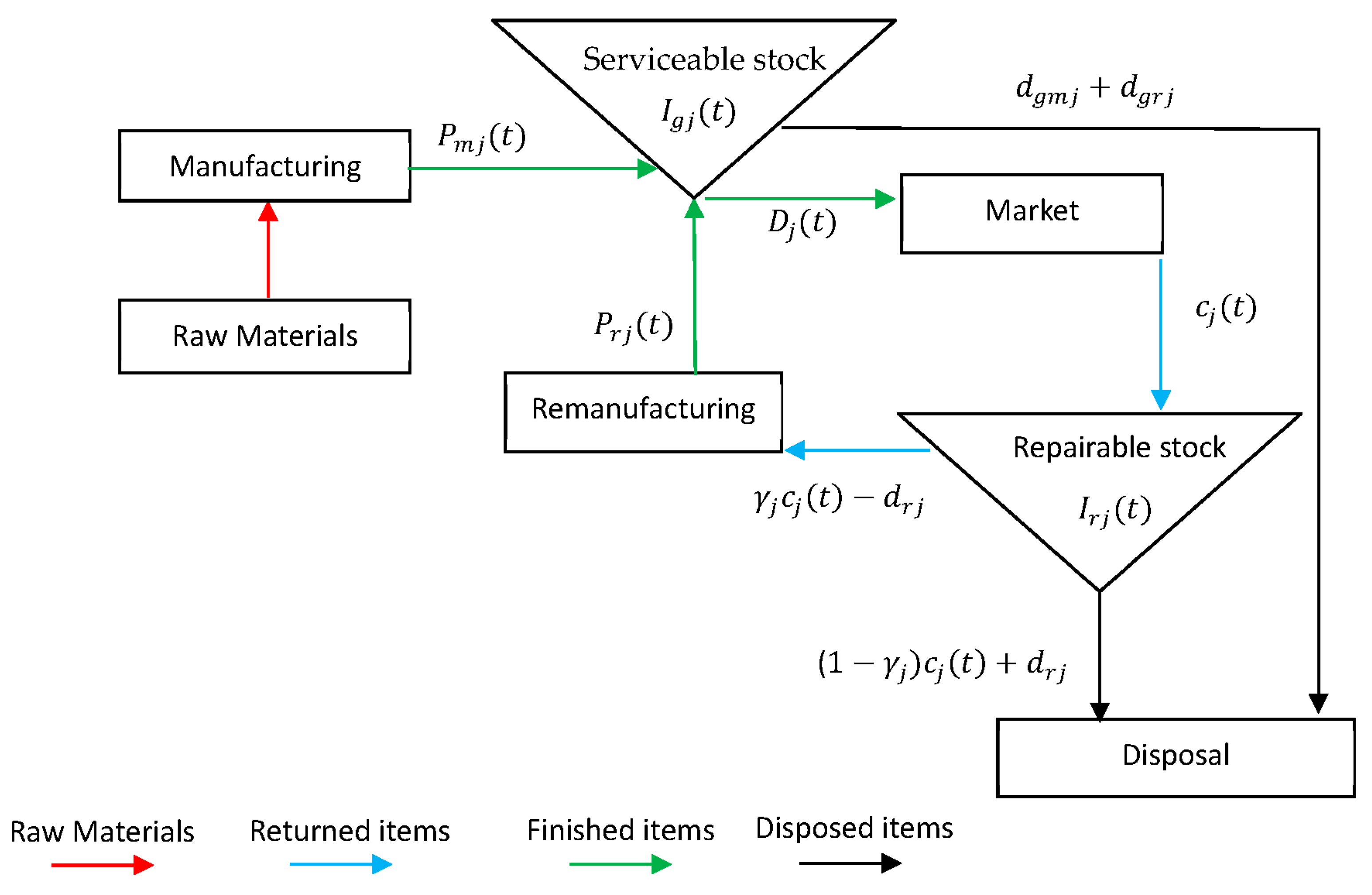
Figure 5.
Inventory variation of manufactured, remanufactured and returned items for one cycle.
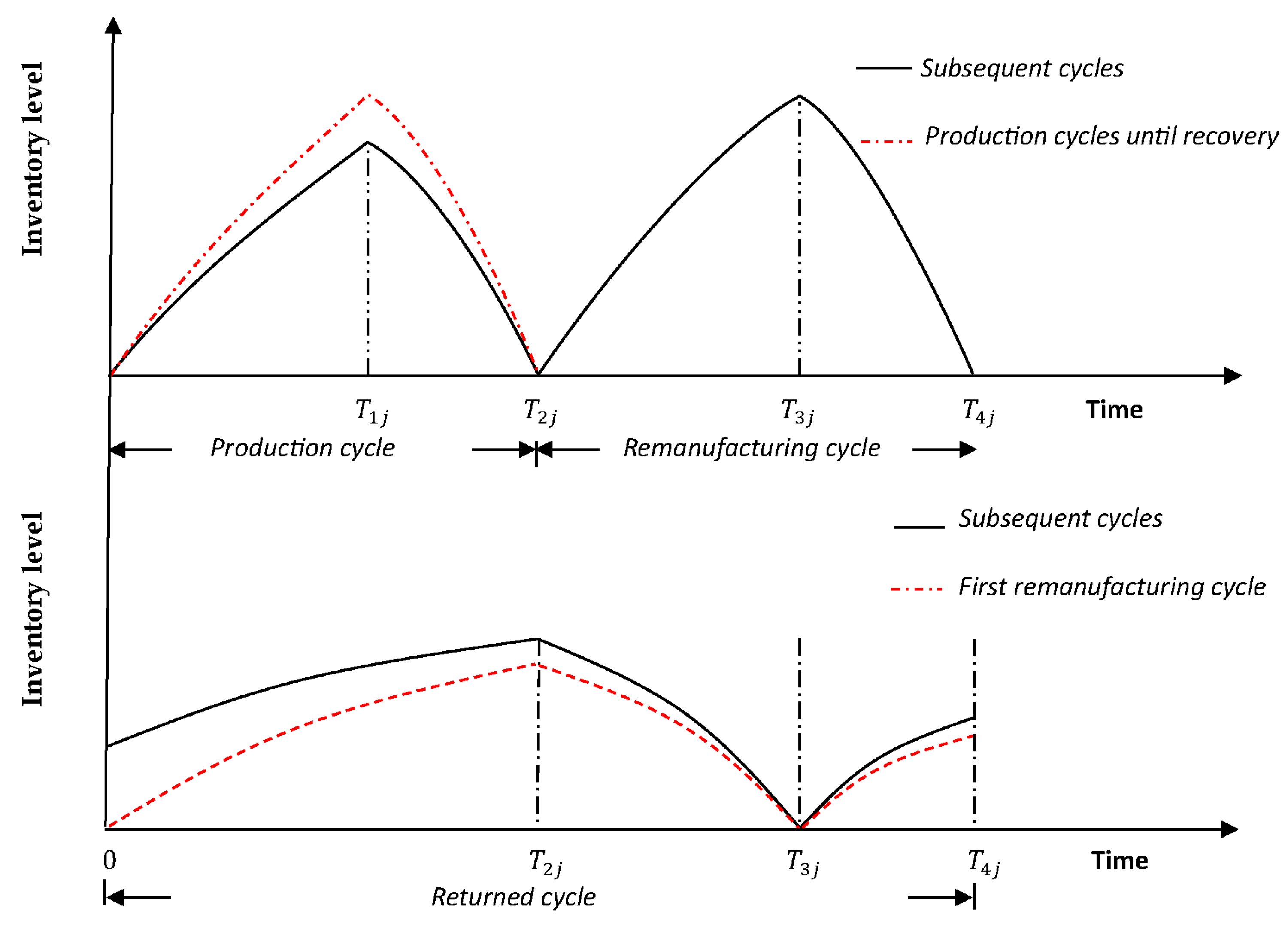
The variations in the inventory levels depicted in Figure 5 are given by the following differential equations:
Considering the boundary conditions, the solutions of the above differential equations are:
respectively, where
From Equations (1)-(14), we note that each function
is solely modelled and, therefore, functions may or may not be related to each
other.
The per cycle total cost components for the
underlying inventory model are given as:
Purchase price for returned items () + Inspection cost () + Disposal cost for waste and deteriorated items
() + Material cost for new items () + Manufacturing cost () + Remanufacturing cost () + Holding costs (+ Switching cost for manufacturing () + Switching costs for remanufacturing () + Investment cost () + Set-up and order costs (=
Now, denote , and .
As can be seen, the returned,
manufacturing and remanufacturing costs cover and include deteriorated items.
This is very well recognised in the literature because items deteriorate while
they are effectively in stock (e.g., Inderfurth et al. 2005; Jaggi et al. 2015;
Alamri et al. 2016; Polotski et al. 2019).
From Equations (8)-(14), the
holding costs are as follows:
Holding costs for produced and remanufactured items
at the serviceable stock:
Holding cost for returned items at the repairable
stock:
Therefore, the per unit time total cost function of
the unified inventory model during the cycle , as a function of denoted by is given by
where
Note that Equation (16) is a modified
version of that of Alamri (2021). Therefore, and to avoid repetition, the
existence, uniqueness and global optimality of the solution can be obtained by
a quite similar way. Interested readers are referred to (Alamri, 2011; 2021).
The variables that minimise given by Equation (16) are governed by the
following relations:
For example, relations 19 and 20 guarantee that the
inventory levels for the production and the remanufacturing phases have equal
values for and for . Note that the term is modelled as a deterministic value, i.e., it
impacts the behaviour of each cycle until the system plateaus. This is a key in
the mathematical formulation and, consequently, it ensures that the model is a
viable solution for each cycle, whether the input parameters change their
values or remain static (Alamri (2021)).
It can be seen from that . Also, from Equation (19), a pure strategy of no manufacturing option. In
this case, . Conversely, . Thus, from Equations (21) and (22), a pure strategy of no remanufacturing option. Conversely, . Thus,
and . Hence, Equations (19)-(22) implies constraint
(18), and, therefore, constraint (18) can be ignored. Thus, our goal is to
solve the following objective function:
4.2.1. Solution procedure
As can be seen from Equations (19)-(22) that can be obtained as functions of , where
Taking also into account Equations (19)-(22), the
objective function is reduced to the
following function with the variable (say
) subject to .
where is given by Equation (15) and is given by Equation (17).
Hence, if , then the necessary condition for having a minimum
for is
where and represent, respectively, the
derivatives of and with respect to .
Now considering Equation (26), then we obtain
Equation (29) can, now, be used to obtain the
optimal value of and its corresponding total minimum cost. Then the
optimal values of can be obtained from Equations
(19)-(22), respectively.
To find the optimal for a given , the following steps are required:
- In the first remanufacturing cycle, start by setting in Equation (29) and compute .
- Repeat step 1 for to compute .
- Set in Equation (29) and compute
- Repeat step 3 for to compute .
- Set in Equation (29) and compute
- Repeat step 5 for to compute .
- Repeat steps 5 and 6 for and to compute
- Set when at its minimum and continue to insert in Equation (29) until the system plateaus.
Remark:
For a mature system, applying the above steps will generate the optimal remanufacturing policy, where represents the current on hand inventory of returned items.
5. Illustrative examples for different sittings
In this section, we present numerical examples and special cases that reflect different realistic situations. Products that may encounter remanufacturing include tyres, motor vehicle parts, electric motors, computers, air-conditioning units, photocopiers, telecommunication equipment, aerospace devices, aircraft parts, gaming machines, medical equipment, vending machines, automotive parts, industrial equipment, televisions, etc. (Statham, 2006). In real life settings, manufacturing, remanufacturing, demand, return and deterioration rates may vary with time or with any other factors (Alamri and Balkhi, 2007; Alamri and Syntetos 2018; Benkherouf et al., 2014; Datta et al., 1998; Grosse et al., 2013; Hariga and Benkherouf, 1994; Karmarkar and Pitbladdo, 1997; Omar and Yeo, 2009; Sana, 2010). Accordingly, the proposed model allows the incorporation of different forms of time-varying functions. Let us now consider the following functions for time-varying rates:
Note that is an increasing function of time.
In real life sitting, all function or input parameters are subject to adjustment due to external competitiveness and/or internal challenges or due to price fluctuations. Therefore, our model is viable if all values are adjusted for subsequent cycles.
The objective function has been coded in MATLAB for the input parameters that are presented in Table 5 below and solutions were obtained using Equation (29) subject to . Note that each of the return, manufacturing and remanufacturing rates is solely modelled. This is so because they may or may not be considered as functions of the demand rate. Now, let us consider the following functions for varying return, manufacturing and remanufacturing rates as functions of the demand rate:
Table 5.
Input parameters for time-varying rates.
| 1.6 | 1.6 | 1.2 | 1000 | 130 | 1666.7 |
| Dollars/unit/month | Dollars/unit/month | Dollars/unit/month | Unit/month | Unit/month | Unit/month |
| 216.7 | 3333.3 | 433.3 | 1 | 1 | 1 |
| Unit/month | Unit/month | Unit/month | Unit/month | Unit/month | Unit/month |
| 50 | 50 | 40 | 0.25 | 0.25 | 0.25 |
| Unit/month | Unit/month | Unit/month | Unit/month | Unit/month | Unit/month |
| 4000 | 100 | 100 | 2400 | 1600 | 1200 |
| Dollars/cycle | Dollars/cycle | Dollars/cycle | Dollars/cycle | Dollars/cycle | Dollars/cycle |
| 0.2 | 2 | 1.2 | 5 | 0.5 | |
| Dollars/unit | Dollars/unit | Dollars/unit | Dollars/unit | Dollars/unit | |
5.1. Example 1
In this example, we investigate the effect of the first remanufacturing cycle on the behaviour of the model with respect to the parameters that are listed in Table 5. In this example, we consider , i.e., the expected number of times an item can be remanufactured on its life cycle is 5. In this case, ) and . The optimal values of until the system plateaus are obtained and the results are shown in Table 6. In the first remanufacturing cycle, we have taken (recall Table 4) resulting in a total number of . This retuned quantity has been accumulated by time at a return rate of or 68.3% of the demand rate. At time , , which constitutes the initial inventory of returned items for the second cycle. The deteriorated quantity in the serviceable stock is and have deteriorated in the repairable stock, i.e., . This deteriorated quantity can be sold at a salvage price or (as in this example) incur a disposal charge. The optimal produced quantity is , which has been accumulated by time to satisfy demand until time (the time by which the remanufacturing process started). The optimal remanufactured quantity is , which has been accumulated by time to satisfy demand until time . The total minimum cost per month is and the total minimum cost for the first remanufacturing cycle is .
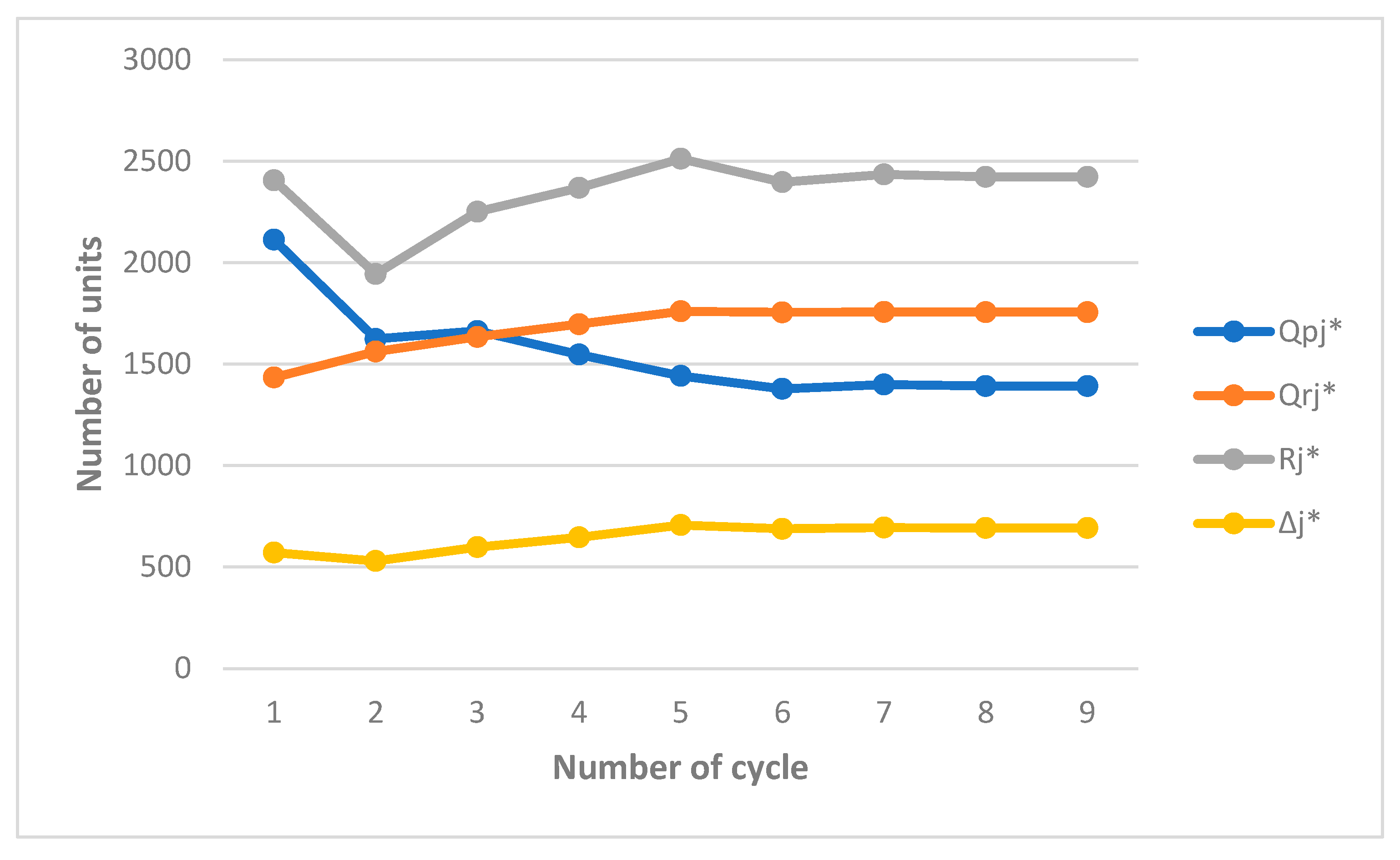
It is worth noting here that in the first remanufacturing cycle, the initial inventory of returned items is zero as there are no returned items to be remanufactured. Accordingly, () attain their minimum (maximum) values in this cycle resulting in a dramatic decrease in the manufactured quantity in the second cycle. Note that, attain their minimum values in the second cycle because of the effect of the first cycle. Moreover, cycles are influenced by and, consequently, the optimal values vary from cycle to cycle and reach their maximum values in the fifth cycle. As a result, approach their minimum values in the sixth cycle before the system plateaus in the eighth cycle (Table 6). Therefore, when the system plateaus, the buyback proportion is set equal to and the use proportion is set equal to , which is equivalent to a reusable proportion or 57.8% of demand rate. Figure 7 depicts the effect of on the behaviour of the optimal values until the system plateaus. As can be seen, in cycles , all returned items have been remanufactured less than or equal to number of times upon recovery and less than or equal to when recovered for subsequent cycles. This implies that the number of times an item can be remanufactured is tangible and tractable. Finally, in cycles , vary from cycle to cycle. Unlike previous works excluding the work of Alamri (2021), this, indeed, constitutes evidence that our model is viable if the values of the input parameters are distinct for subsequent cycles.
As illustrated in example 1, other forms of varying functions can be disseminated from the general formulation to assess the consequences of distinct strategies.
Table 6.
Optimal results for varying rates when .
| 1 | 1 | 2821 | 1.474 | 0.849 | 0.683 | 2.954 | 2113 | 1434 | 2406 | 571 | 65 | 11332 | 33475 |
| 2 | 2 | 3727 | 1.305 | 0.807 | 0.614 | 2.692 | 1624 | 1562 | 1944 | 530 | 69 | 11155 | 30031 |
| 3 | 3 | 3952 | 1.147 | 0.778 | 0.688 | 2.773 | 1663 | 1634 | 2251 | 598 | 74 | 11206 | 31077 |
| 4 | 4 | 3994 | 1.001 | 0.758 | 0.736 | 2.733 | 1547 | 1697 | 2369 | 646 | 75 | 11081 | 30287 |
| 5 | 5 | 3999 | 0.868 | 0.745 | 0.791 | 2.702 | 1442 | 1760 | 2512 | 707 | 76 | 10948 | 29582 |
| 6 | 5 | 3999 | 0.868 | 0.745 | 0.771 | 2.652 | 1378 | 1755 | 2397 | 688 | 75 | 10895 | 28891 |
| 7 | 5 | 3999 | 0.868 | 0.745 | 0.778 | 2.668 | 1399 | 1757 | 2435 | 694 | 75 | 10912 | 29117 |
| 8 | 5 | 3999 | 0.868 | 0.745 | 0.776 | 2.663 | 1392 | 1756 | 2423 | 692 | 75 | 10907 | 29046 |
| 9 | 5 | 3999 | 0.868 | 0.745 | 0.776 | 2.663 | 1392 | 1756 | 2423 | 692 | 75 | 10907 | 29046 |
Figure 7.
The effect of model parameters on the optimal values when .
5.2. Example 2
In this example, we replicate example 1 to observe the behaviour of the optimal values when . As can be seen from Table 7, the optimal values behave similarly when the expected number of times an item can be remanufactured on its life cycle decreases from 3 to 5. The only exception is that the value of in the third cycle experiences a slight decrease by 10 units from that accumulated in the first cycle. This can be justified by the fact that the value of in the second cycle is greater than that accumulated in the first cycle (see Table 6). Note that reach their maximum values in the third cycle and approach their minimum values in the fourth cycle before the system plateaus in the eighth cycle (Table 7).
Table 7.
Optimal results for varying rates when .
| 1 | 1 | 3009 | 1.238 | 0.788 | 0.770 | 2.981 | 2089 | 1498 | 2741 | 623 | 66 | 11324 | 33761 |
| 2 | 2 | 3845 | 0.983 | 0.749 | 0.736 | 2.684 | 1497 | 1679 | 2320 | 632 | 73 | 11006 | 29544 |
| 3 | 3 | 3986 | 0.765 | 0.730 | 0.855 | 2.716 | 1415 | 1806 | 2731 | 768 | 77 | 10885 | 29565 |
| 4 | 3 | 3986 | 0.765 | 0.730 | 0.808 | 2.604 | 1277 | 1793 | 2460 | 721 | 74 | 10770 | 28049 |
| 5 | 3 | 3986 | 0.765 | 0.730 | 0.825 | 2.645 | 1325 | 1798 | 2558 | 738 | 75 | 10811 | 28592 |
| 6 | 3 | 3986 | 0.765 | 0.730 | 0.819 | 2.630 | 1308 | 1796 | 2522 | 732 | 75 | 10796 | 28398 |
| 7 | 3 | 3986 | 0.765 | 0.730 | 0.821 | 2.636 | 1315 | 1797 | 2535 | 734 | 75 | 10801 | 28473 |
| 8 | 3 | 3986 | 0.765 | 0.730 | 0.820 | 2.634 | 1312 | 1797 | 2530 | 733 | 75 | 10800 | 28444 |
| 9 | 3 | 3986 | 0.765 | 0.730 | 0.820 | 2.634 | 1312 | 1797 | 2530 | 733 | 75 | 10800 | 28444 |
5.3. Example 3
In this example, we repeat example 2 by increasing the investment cost, from 4000 dollars to 6000 dollars to investigate the behaviour of the optimal values. Table 8 reveals that the optimal situation in this case is to remanufacture once (). Note that remain static until the system plateaus and, consequently, the only factor affecting the optimal values is . As can be seen from Table 8, the model behaves similarly with respect to that reach their maximum values in the first cycle and attain their minimum values in the second cycle before the system plateaus in the sixth cycle (Table 8). Note that () reach their minimum (maximum) values in the first cycle since the inventory of returned items is zero (see also Table 6 and Table 7). It is worth noting here that (recall solution steps). However, when the system plateaus for , the difference between the total minimum cost per month is negligible, i.e., .
Table 8.
Optimal results for varying rates when .
| 1 | 1 | 4514 | 1.238 | 0.788 | 0.754 | 3.224 | 2318 | 1614 | 2940 | 656 | 79 | 11809 | 38073 |
| 2 | 1 | 4514 | 1.238 | 0.788 | 0.615 | 2.768 | 1647 | 1644 | 2010 | 545 | 77 | 11351 | 31421 |
| 3 | 1 | 4514 | 1.238 | 0.788 | 0.645 | 2.859 | 1772 | 1645 | 2187 | 571 | 78 | 11446 | 32730 |
| 4 | 1 | 4514 | 1.238 | 0.788 | 0.638 | 2.838 | 1743 | 1645 | 2145 | 565 | 78 | 11424 | 32425 |
| 5 | 1 | 4514 | 1.238 | 0.788 | 0.640 | 2.843 | 1749 | 1644 | 2154 | 567 | 78 | 11429 | 32489 |
| 6 | 1 | 4514 | 1.238 | 0.788 | 0.639 | 2.843 | 1749 | 1645 | 2153 | 567 | 78 | 11428 | 32487 |
| 7 | 1 | 4514 | 1.238 | 0.788 | 0.639 | 2.843 | 1749 | 1645 | 2153 | 567 | 78 | 11428 | 32487 |
5.4. Special cases
Case 1: In this case (Case1), we replicate Table 6 and Table 7 to investigate the work of Alamri (2021) for the set of input parameters as listed in Table 5. In Case 1, we let , which are identical with that of Alamri (2021). Note that and an item is recovered an indefinite number of times. By substituting the above values in Equation (29) until the system plateaus, the results are obtained as shown in Table 9. As can be seen, Table 9 is identical with Table 3 page 529 in Alamri (2021). This constitutes evidence that ensures the validity and robustness of our general model.
Table 9.
Optimal results for varying rates as in Alamri (2021) with .
| 1 | 2.454 | 2373 | 493 | 657 | 69 | 33 | 10317 | 25314 |
| 2 | 2.371 | 2223 | 533 | 632 | 75 | 34 | 10220 | 24231 |
| 3 | 2.364 | 2210 | 536 | 630 | 75 | 34 | 10211 | 24140 |
| 4 | 2.364 | 2210 | 536 | 630 | 75 | 34 | 10211 | 24140 |
Case 2: In this case (Case2), we investigate the behaviour of the model when the demand rate is adjusted within cycles. In real life sitting, all function or input parameters are subject to adjustment due to external competitiveness and/or internal challenges or due to price fluctuations. Let us now support our finding in Example 1 and show the validity of our model if the input parameters change their values for subsequent cycles. In Case 2, we will illustrate how the system would behave if the decision maker wished to increase the demand rate in the eighth cycle to evaluate the consequences of such increase. In Case 2, we assume that , where . Note that row one of Table 10 represents the results derived for the eighth cycle for example 2 (see Table 7). A comparison between Table 7 and Table 10 reveals that in the first cycle of the adjustment, all optimal values increase except that encounters a slight decrease. Such increase can be justified by the increase of . Note that all decision variables attain their maximum (minimum) values in the ninth (tenth) cycle, i.e., in the first (second) cycle of the adjustment of the demand rate.
Table 10.
Optimal results for varying rates when .
| 8* | 3 | 3986 | 0.765 | 0.730 | 0.820 | 2.634 | 1312 | 1797 | 2530 | 733 | 75 | 10800 | 28444 |
| 9 | 3 | 3986 | 0.765 | 0.730 | 0.936 | 2.488 | 1353 | 2139 | 3248 | 912 | 76 | 12099 | 30106 |
| 10 | 3 | 3986 | 0.765 | 0.730 | 0.884 | 2.340 | 1154 | 2104 | 2860 | 847 | 71 | 11925 | 27908 |
| 11 | 3 | 3986 | 0.765 | 0.730 | 0.905 | 2.396 | 1228 | 2118 | 3007 | 873 | 74 | 11992 | 28737 |
| 12 | 3 | 3986 | 0.765 | 0.730 | 0.897 | 2.375 | 1200 | 2113 | 2950 | 863 | 73 | 11966 | 28419 |
| 13 | 3 | 3986 | 0.765 | 0.730 | 0.900 | 2.383 | 1210 | 2115 | 2971 | 866 | 73 | 11976 | 28538 |
| 14 | 3 | 3986 | 0.765 | 0.730 | 0.899 | 2.380 | 1205 | 2115 | 2965 | 866 | 73 | 11972 | 28489 |
| 15 | 3 | 3986 | 0.765 | 0.730 | 0.899 | 2.380 | 1205 | 2115 | 2965 | 866 | 73 | 11972 | 28489 |
Case 3: In this case (Case3), we replicate example 2 to investigate the behaviour of the optimal values in different settings. Row one of Table 11 (base model) denotes the results of the first cycle for example 2 (see Table 7). Table 11 illustrates the effect of distinct model parameter on the behaviour of the optimal values to compare the results with that derived for example 2. Note that in all cases, the model behaves as expected. For example, when the holding costs are equal, i.e., , all optimal values are higher than those of the base model, except the total minimum cost per unit time that experiences a lower cost. This can be justified by the fact that the system reduces the holding cost at the serviceable stock. Note that similar behaviour is also observed for except the fraction of returned items that is associated with a slight decrease. This can be attributed to the increase of the order cost for returned items. Similarly, when , which also affecting , all optimal values are higher than those of the base model except the cycle length and the produced quantity that are associated with lower values. This can be attributed to the fact that the fraction of returned items increased by 7.8% . For , we note that are associated with greater values than those of the base model, and are associated with lower values. This can be justified by the fact that the system reaps the benefit of not disposing more items. Finally, when the deterioration rates are equal, i.e., , all optimal values are less than those of the base model, except the total minimum cost per unit time and the fraction of returned items that are associated with greater values. As expected, more items (97 units) are deteriorated and disposed outside the system due to the increase of the deterioration rates.
Table 11.
Sensitivity analysis of the optimal results for varying rates when .
| Parameters | ||||||||||||||
|---|---|---|---|---|---|---|---|---|---|---|---|---|---|---|
| Base model* | 1 | 1 | 3009 | 1.238 | 0.788 | 0.770 | 2.981 | 2089 | 1498 | 2741 | 623 | 66 | 11324 | 33761 |
| 1 | 1 | 3009 | 1.238 | 0.788 | 0.772 | 3.090 | 2178 | 1564 | 2866 | 652 | 72 | 11139 | 34420 | |
| 1 | 1 | 3009 | 1.238 | 0.788 | 0.761 | 3.113 | 2212 | 1561 | 2849 | 641 | 73 | 11586 | 36072 | |
| 1 | 1 | 3009 | 1.486 | 0.788 | 0.835 | 2.888 | 1926 | 1530 | 2866 | 690 | 65 | 12244 | 35364 | |
| 1 | 1 | 3009 | 1.238 | 0.788 | 0.760 | 2.982 | 2104 | 1484 | 2705 | 609 | 66 | 11345 | 33832 | |
| 1 | 1 | 3009 | 1.238 | 0.788 | 0.778 | 2.950 | 2074 | 1486 | 2737 | 618 | 97 | 11377 | 33564 |
* Row one of Table 7.
Case 4: In this case (Case 4), we replicate example 2 with respect to constant rates without deterioration. As can be seen from Table 12, the model behaves in a similar way as that observed in Table 7. In particular, the behaviour of in the third cycle and in the second cycle (recall the justification in example 2). Note that attains its maximum value when the system plateaus, i.e., it differs from that observed in Table 7. A comparison between Table 7 and Table 12 shows that for each cycle , all optimal values are higher than those of example 2 (Table 7), except that are associated with lower values.
Table 12.
Optimal results for constant rates without deterioration when .
| 1 | 1 | 3009 | 1.238 | 0.788 | 0.635 | 4.808 | 3207 | 1781 | 3051 | 623 | 9479 | 45577 |
| 2 | 2 | 3845 | 0.983 | 0.749 | 0.736 | 4.257 | 2277 | 1980 | 2685 | 655 | 9362 | 39851 |
| 3 | 3 | 3986 | 0.765 | 0.730 | 0.717 | 4.225 | 2128 | 2097 | 3028 | 768 | 9264 | 39138 |
| 4 | 3 | 3986 | 0.765 | 0.730 | 0.695 | 4.071 | 1980 | 2091 | 2829 | 743 | 9218 | 37532 |
| 5 | 3 | 3986 | 0.765 | 0.730 | 0.700 | 4.107 | 2014 | 2093 | 2875 | 749 | 9229 | 37906 |
| 6 | 3 | 3986 | 0.765 | 0.730 | 0.699 | 4.099 | 2006 | 2092 | 2864 | 747 | 9227 | 37816 |
| 7 | 3 | 3986 | 0.765 | 0.730 | 0.699 | 4.101 | 2008 | 2093 | 2867 | 748 | 9227 | 37837 |
| 8 | 3 | 3986 | 0.765 | 0.730 | 0.820 | 4.100 | 2008 | 2093 | 2866 | 748 | 9227 | 37832 |
| 9 | 3 | 3986 | 0.765 | 0.730 | 0.820 | 4.100 | 2008 | 2093 | 2866 | 748 | 9227 | 37832 |
Case 5: In this case (Case 5), we replicate example 3 with respect to constant rates without deterioration. As Table 13 shows, the model behaves similarly with respect to constant rates without deterioration (see Table 8). As can be seen from Table 13, reach their maximum values in the first cycle and attain their minimum values in the second cycle before the system plateaus in the fifth cycle (Table 13). Similarly, () reach their minimum (maximum) values in the first cycle since the inventory of returned items is zero. A comparison between Table 8 and Table 13 shows that for each cycle , all optimal values are higher than those of example 3 (Table 8), except that are associated with lower values. Note that this finding is also observed in Case 4. In addition, (recall solution steps). However, when the system plateaus for , the difference between the total minimum cost per month is negligible, i.e., (see also example 3).
Table 13.
Optimal results for constant rates without deterioration when .
| 1 | 1 | 4514 | 1.238 | 0.788 | 0.614 | 5.243 | 3348 | 1895 | 3219 | 642 | 9779 | 51268 |
| 2 | 1 | 4514 | 1.238 | 0.788 | 0.534 | 4.476 | 2526 | 1950 | 2390 | 574 | 9603 | 42983 |
| 3 | 1 | 4514 | 1.238 | 0.788 | 0.544 | 4.568 | 2620 | 1949 | 2486 | 585 | 9628 | 43984 |
| 4 | 1 | 4514 | 1.238 | 0.788 | 0.543 | 4.554 | 2605 | 1949 | 2471 | 583 | 9624 | 43828 |
| 5 | 1 | 4514 | 1.238 | 0.788 | 0.543 | 4.556 | 2607 | 1949 | 2474 | 584 | 9625 | 43852 |
| 6 | 1 | 4514 | 1.238 | 0.788 | 0.543 | 4.556 | 2607 | 1949 | 2474 | 584 | 9625 | 43852 |
6. Implications and managerial insights
Considering that returned items may arrive with different number of remanufacturing times reduces the total system cost as well as ensures reducing the disposal of unnecessary amount.
The optimal policy is either to remanufactured once or remanufactured up to the expected number of times an item can be remanufactured on its life cycle.
All function may or may not be related to each other and, therefore, each is solely modelled.
The number of times an item can be remanufactured is definite, tractable and modelled.
The purchasing price of recovery items, remanufacturing investment cost, return rate and the percentage of returns vary until the number of cycles reaches the expected number of times an item can be remanufactured on its life cycle. Such variation implies further reduction in the total cost and ensures a positive environmental impact.
The return rate is a varying demand dependent rate, which is a decision variable. This consideration reduces the total cost and solid waste disposal and, consequently, the system emphasises sustainability because it reflects the influence of economic, social and environmental interests.
The initial inventory of returned items in the first remanufacturing cycle is zero and it differs from cycle to cycle, which in turn implies that the optimal values also vary until the system plateaus. This consideration is key in that it allows for the adjustment of all functions and input parameters for subsequent cycles.
The proposed model is a viable solution for different forms of time-varying functions that can be disseminated from the general formulation as well as for systems encountering periodic review applications.
The solution quality of the special cases is identical with that of published sources, i.e., the validity and robustness of the general model are ascertained.
7. Summary and conclusion
In this paper, we have been concerned with the implications of the number of times an item can be remanufactured. The mathematical modelling of reverse logistics inventory systems assumes that all returned items have been remanufactured with an equal number of times. Nevertheless, this assumption ignores the fact that returned items may arrive out of sequence. The present paper developed a new mathematical expression of the percentage of returns that can be remanufactured a finite number of times. The proposed expression has been modelled as a function of the expected number of times an item can be remanufactured on its life cycle and the number of times an item can be technologically (or optimally) remanufactured based on its quality upon recovery. The mathematical expression has been incorporated in a general joint model for production and remanufacturing options.
In the proposed model, demand, product deterioration, production and remanufacturing rates are arbitrary functions of time so as to reflect a diverse range of time-varying forms. The return rate is a varying demand dependent rate, which is a decision variable. The model considers the initial inventory of returned items in the mathematical formulation, which enables decision makers to adjust all functions and input parameters for subsequent cycles.
We evaluated the impact of varying rates on the optimal quantities subject to the expected number of times an item can be remanufactured on its life cycle. We found that the effect of varying purchasing price of recovery items, remanufacturing investment cost, return rate, the percentage of returns and the initial inventory of returned items significantly impact on the behaviour of the model. Consequently, the optimal policy is either to remanufactured once or remanufactured up to the expected number of times an item can be remanufactured on its life cycle. We tested and observed the behaviour of the model in different realistic situations and discussed some important managerial insights for decision makers. The versatile nature of the proposed model has been emphasised, where the viability, validity and robustness of the proposed model are ascertained.
Further research may include extensions such as allowing for shortages, incorporating learning and forgetting curves in the manufacturing and remanufacturing rates. In addition, the formulation of greenhouse gas (GHG) emissions from manufacturing, remanufacturing and transportation, as well as energy consumption during manufacturing and remanufacturing processes can also be addressed. In parallel, it seems plausible to extend the general model for multiple manufacturing and remanufacturing cycles while accounting for different emission trading schemes.
References
- Alamri, A. A., & Balkhi, Z. T. (2007). The effects of learning and forgetting on the optimal production lot size for deteriorating items with time varying demand and deterioration rates. International Journal of Production Economics, 107 (1), 125-138. [CrossRef]
- Alamri, A. A. (2011). Theory and methodology on the global optimal solution to a General Reverse Logistics Inventory Model for deteriorating items and time-varying rates. Computers & Industrial Engineering, 60 (2), 236-247. [CrossRef]
- Alamri, A. A., Harris, I., & Syntetos, A. A. (2016). Efficient inventory control for imperfect quality items. European Journal of Operational Research, 254 (1), 92-104. [CrossRef]
- Alamri, A. A., & Syntetos, A. A. (2018). Beyond LIFO and FIFO: Exploring an Allocation-In-Fraction-Out (AIFO) policy in a two-warehouse inventory model. International journal of production economics, 206, 33-45. [CrossRef]
- Alamri, A. A. (2021). Exploring the effect of the first cycle on the economic production quantity repair and waste disposal model. Applied Mathematical Modelling, 89 (1), 519-540. [CrossRef]
- Andrade, R. P., Lucato, W. C., Vanalle, R. M., & Vieira Junior, M. (2013). Reverse logistics and competitiveness: a brief review of this relationship. In POMS ANNUAL CONFERENCE, 24th.
- Bazan, E., Jaber, M. Y., & El Saadany, A. M. (2015). Carbon emissions and energy effects on manufacturing–remanufacturing inventory models. Computers & Industrial Engineering, 88, 307-316. [CrossRef]
- Bazan, E., Jaber, M. Y., & Zanoni, S. (2016). A review of mathematical inventory models for reverse logistics and the future of its modeling: An environmental perspective. Applied Mathematical Modelling, 40 (5), 4151-4178. [CrossRef]
- Bei, W., & Linyan, S. (2005). A review of reverse logistics. Applied Sciences, 7 (1), 16-29.
- Benkherouf, L., Konstantina, S., & Konstantaras, L. (2014). Optimal lot sizing for a production-recovery system with time-varying demand over a finite planning horizon. IMA Journal of Management Mathematics, 25, (4) 403–420. [CrossRef]
- Bras, B. (2007). “Design for Remanufacturing Processes.” In Environmentally Conscious Mechanical Design, edited by M.Kutz. Hoboken, NJ: John Wiley & Sons.
- Cao, J., Chen, X., Zhang, X., Gao, Y., Zhang, X., & Kumar, S. (2020). Overview of remanufacturing industry in China: Government policies, enterprise, and public awareness. Journal of Cleaner Production, 242, 118450. [CrossRef]
- Datta, T.K., Paul, K., & Pal, A.K. (1998). Demand promotion by upgradation under stock-dependent demand situation–a model. International Journal of Production Economics 55 (1), 31–38. [CrossRef]
- De Brito, M. P., & Dekker, R. (2004). A framework for reverse logistics (pp. 3-27). Springer Berlin Heidelberg. [CrossRef]
- Dobos, I., & Richter, K. (2000). The integer EOQ repair and waste disposal model--further analysis. Central European Journal of Operations Research, 8 (2), 173-194.
- Dobos, I., & Richter, K. (2003). A production/recycling model with stationary demand and return rates. Central European Journal of Operations Research, 11 (1), 35–46.
- Dobos, I., & Richter, K. (2004). An extended production/recycling model with stationary demand and return rates. International Journal of Production Economics, 90 (3), 311–323. [CrossRef]
- Dobos, I., & Richter, K. (2006). A production/recycling model with quality considerations. International Journal of Production Economics, 104 (2), 571– 579. [CrossRef]
- El Saadany, A. M. A., & Jaber, M. Y. (2008). The EOQ repair and waste disposal model with switching costs. Computers & Industrial Engineering, 55 (1), 219–233. [CrossRef]
- El Saadany, A. M. A., & Jaber, M. Y. (2010). A production/remanufacturing inventory model with price and quality dependant return rate. Computers & Industrial Engineering, 58 (3), 352–362. [CrossRef]
- El Saadany, A. M., Jaber, M. Y., & Bonney, M. (2013). How many times to remanufacture?. International Journal of Production Economics, 143 (2), 598-604. [CrossRef]
- Flapper, S. D., van Nunen, J., & Van Wassenhove, L. N. (Eds.). (2005). Managing closed-loop supply chains. Springer Science & Business Media. [CrossRef]
- Fleischmann, M. (2001). Reverse logistics network structures and design (No. ERS-2001-52-LIS). ERIM Report Series Research in Management.
- Fleischmann, M., Bloemhof-Ruwaard, J. M., Dekker, R., Van der Laan, E., Van Nunen, J. A., & Van Wassenhove, L. N. (1997). Quantitative models for reverse logistics: A review. European Journal of Operational Research, 103 (1), 1-17. [CrossRef]
- Govindan, K., Soleimani, H., & Kannan, D. (2015). Reverse logistics and closed-loop supply chain: A comprehensive review to explore the future. European journal of operational research, 240 (3), 603-626. [CrossRef]
- Grosse, E. H., Glock, C. H., & Jaber, M. Y. (2013). The effect of worker learning and forgetting on storage reassignment decisions in order picking systems. Computers & Industrial Engineering, 66 (4), 653-662. [CrossRef]
- Guide, V. D. R., Harrison, T. P., & Van Wassenhove, L. N. (2003). The challenge of closed-loop supply chains. Interfaces, 33 (6), 3-6. [CrossRef]
- Hariga, M., & Benkherouf, L. (1994). Optimal and heuristic inventory replenishment models for deteriorating items with exponential time-varying demand. European Journal of Operational Research 79 (1), 123–137. [CrossRef]
- Inderfurth, K., Lindner, G., & Rachaniotis, N. P. (2005). Lot sizing in a production system with rework and product deterioration. International Journal of Production Research, 43 (7), 1355–1374. [CrossRef]
- Jaber, M. Y., & El Saadany, A. M. A. (2009). The production, remanufacture and waste disposal model with lost sales. International Journal of Production Economics, 120 (1), 115–124. [CrossRef]
- Jaggi, C. K., Tiwari, S., & Shafi, A. (2015). Effect of deterioration on two-warehouse inventory model with imperfect quality. Computers & Industrial Engineering, 88, 378-385. [CrossRef]
- Karmarkar, U., & Pitblado, R.U. (1997). Quality, class, and competition. Management Science 43 (1), 27–39. [CrossRef]
- Kozlovskaya, N., Pakhomova, N., & Richter, K. (2017). A note on “The EOQ repair and waste disposal model with switching costs”. Computers & Industrial Engineering, 103, 310-315. [CrossRef]
- Liu, Z., Diallo, C., Chen, J., & Zhang, M. (2020). Optimal pricing and production strategies for new and remanufactured products under a non-renewing free replacement warranty. International Journal of Production Economics, 226, 107602. [CrossRef]
- Montabon, F., Pagell, M., & Wu, Z. (2016). Making sustainability sustainable. Journal of Supply Chain Management, 52 (2), 11-27. [CrossRef]
- NAHMIASJ, S., & Rivera, H. (1979). A deterministic model for a repairable item inventory system with a finite repair rate. International Journal of Production Research, 17 (3), 215-221. [CrossRef]
- Modak, N. M., Sinha, S., & Ghosh, D. K. (2023). A review on remanufacturing, reuse, and recycling in supply chain—Exploring the evolution of information technology over two decades. International Journal of Information Management Data Insights, 3 (1), 100160.
- Omar, M., & Yeo, I. (2009). A model for a production–repair system under a time- varying demand process. International Journal of Production Economics, 119 (1), 17–23. [CrossRef]
- Polotski, V., Kenne, J. P., & Gharbi, A. (2019). Joint production and maintenance optimization in flexible hybrid Manufacturing–Remanufacturing systems under age-dependent deterioration. International Journal of Production Economics, 216, 239-254. [CrossRef]
- Richter, K. (1996a). The EOQ repair and waste disposal model with variable setup numbers. European Journal of Operational Research, 95 (2), 313-324. [CrossRef]
- Richter, K. (1996b). The extended EOQ repair and waste disposal model. International Journal of Production Economics, 45 (1-3), 443-447. [CrossRef]
- Richter, K. (1997). Pure and mixed strategies for the EOQ repair and waste disposal problem. Operations-Research-Spektrum, 19 (2), 123-129. [CrossRef]
- Richter, K., & Dobos, I. (1999). Analysis of the EOQ repair and waste disposal problem with integer setup numbers. International Journal of Production Economics, 59 (1), 463-467. [CrossRef]
- Rogers, D. S., & Tibben-Lembke, R. (2001). An examination of reverse logistics practices. Journal of Business Logistics, 22 (2), 129-148. [CrossRef] [PubMed]
- Rubio, S., & Jiménez-Parra, B. (2017). Reverse logistics: Concept, evolution and marketing challenges. In Optimization and decision support systems for supply chains (pp. 41-61). Springer International Publishing. [CrossRef]
- Sana, S.S. (2010). An economic production lot size model in an imperfect production system. European Journal of Operational Research, 201 (1) 158–170. [CrossRef]
- Schrady, D. A. (1967). A deterministic inventory model for reparable items. Naval Research Logistics Quarterly, 14 (3), 391-398. [CrossRef]
- Statham, S. (2006). Remanufacturing towards a more sustainable future. Electronics-enabled Products Knowledge-transfer Network, 4.
- Teunter, R. H. (2001). Economic order quantities for recoverable item inventory system. Naval Research Logistics, 48 (6), 484–495. [CrossRef]
- Van Nguyen, T., Zhou, L., Chong, A. Y. L., Li, B., & Pu, X. (2020). Predicting customer demand for remanufactured products: A data-mining approach. European Journal of Operational Research, 281(3), 543-558. [CrossRef]
- Wang, Y., Jiang, Z., Hu, X., & Li, C. (2020). Optimization of reconditioning scheme for remanufacturing of used parts based on failure characteristics. Robotics and Computer-Integrated Manufacturing, 61, 101833. [CrossRef]
Disclaimer/Publisher’s Note: The statements, opinions and data contained in all publications are solely those of the individual author(s) and contributor(s) and not of MDPI and/or the editor(s). MDPI and/or the editor(s) disclaim responsibility for any injury to people or property resulting from any ideas, methods, instructions or products referred to in the content. |
© 2023 by the authors. Licensee MDPI, Basel, Switzerland. This article is an open access article distributed under the terms and conditions of the Creative Commons Attribution (CC BY) license (http://creativecommons.org/licenses/by/4.0/).
Copyright: This open access article is published under a Creative Commons CC BY 4.0 license, which permit the free download, distribution, and reuse, provided that the author and preprint are cited in any reuse.


