Submitted:
28 October 2025
Posted:
13 November 2025
You are already at the latest version
Abstract
The aging of three-layer polyethylene-coated buried steel pipelines for oil/gas and water transport poses significant challenges for public safety, environmental integrity, and economic sustainability. Over time, these pipelines become increasingly susceptible to corrosion and eventual failures, which can lead to environmental hazards, safety risks, and costly repairs. Consequently, predicting the service life of polyethylene-coated steel pipelines is critical for mitigating corrosion risks, extending operational lifespan, and planning effective maintenance strategies. Current international standards lack clear methodologies and criteria for assessing the aging behavior of polyethylene-coated underground pipelines. The current studies have examined two techniques—Line Current Attenuation (LCA) and Drainage Test (DT)—to estimate aging rates in polyolefin-coated pipelines following soil exposure during service. The present study introduces an innovative approach for evaluating aging behavior. It includes a comprehensive analysis using an exponential aging model to estimate the coating's average specific electrical resistance at any service time, as well as quantitative criteria for the failure of oil/gas and water pipelines. Moreover, it is based on the modified LCA as the most suitable aging methodology with some limitations. Finally, the study concludes with a derived correlation between the coating's initial specific electrical resistance and its aging rates, and the prediction of the residual life of the polyethylene coating.
This integrated framework provides a robust foundation for regulatory bodies, design engineers, maintenance planners, quality assurance/control teams, and researchers to ensure the long-term integrity and sustainability of underground polyethylene-coated steel pipelines.
Keywords:
aging model
; underground steel pipeline
; coating’s average specific electrical resistance
; soil corrosion
; three-layer high-density polyethylene coating (3LPE)
; line current attenuation test
; drainage test (cathodic polarization)
1. Introduction
The network of oil, gas, water, and hazardous liquid products pipelines plays a significant role in global infrastructure. One key challenge for underground pipelines is maintaining their integrity throughout their operational life while exposed to soil conditions.
Aging of polyethylene-coated underground steel pipelines poses significant risks and challenges to safety, environmental sustainability, and economic worth. As these pipelines age, they become increasingly susceptible to corrosion, leaks, and failures, leading to environmental disasters and costly repairs. For instance, the USA contains a well-developed network of natural gas pipelines that totals over 300,000 miles (483,000 km). Approximately 62% of these pipelines have been in operation for more than 50 years, nearing their maximum service life or having already surpassed their expected lifetime [1,2]. This situation heightens the likelihood of pipeline accidents and corrosion failures, as verified by statistical data [3,4]. Corrosion remains one of the most common causes of pipeline failures. Data from the Pipeline and Hazardous Materials Safety Administration (PHMSA) in the USA indicates that between 1998 and 2017, approximately 18% of incidents involving gas pipelines (gas transmission, gas gathering, and hazardous liquid pipelines) were caused by corrosion (internal and external) [2]. Another similar organization, the European Gas Pipeline Incident Data Group (EGIG), reported that over the last ten years, corrosion has been the predominant factor in the reported pipeline incidents [3]. In water infrastructure, corrosive soil conditions are the most common cause of external corrosion, accounting for 59% of water transmission mains and 67% of distribution pipelines [4].
As a result, assessing and predicting the durability of polymer-coated steel pipelines, particularly in soil environments, is a key priority for minimizing corrosion risks and forecasting their periodic repairs.
Considerable resources are being devoted to extending the lifespan of pipelines made from various materials, such as steel or concrete (PCCP - Prestressed Concrete Cylinder Pipe) [5,6,7]. Significant achievements include the development of diagnostic methodologies, methods for assessing residual strength, repair methods, software, databases, and regulatory documents employed by operational organizations [8,9,10,11,12,13].
Progress in providing reliable protection for pipelines against soil corrosion has been limited due to several unresolved challenges, including predicting the condition and performance of the polymer coating over time [14,15].
The coating’s performance is influenced by multiple factors, including service temperature, soil conditions and properties, cover depth, properties of local and backfilling materials, and other technical characteristics [16,17,18,19]. During the long-term use of underground pipelines in soil conditions that are designed to last 50 years or more, the coating’s dielectric properties tend to degrade over time, leading to decreasing in its protective properties and electrical resistance and, consequently, to increasing electrical currents at the impressed cathodic protection stations and to raising corrosion risks [20,21,22,23,24].
The efficiency of protective coatings for underground pipelines is evaluated based on their ability to sustain their properties throughout their service life. The predominant properties of the protective coatings include electrical resistance, dielectric continuity, specific defect ratio, and adhesion strength [25]. The evaluation results of the coating’s effectiveness determine whether to proceed with its operation or undertake the required repairs.
Forecasting the polymer coating’s condition and performance over time should consider aging, periodic inspection findings, and technical characteristics along the surveyed pipeline [26]. This is essential for ensuring effective rehabilitation, repair, or replacement planning [27,28]. Consequently, solving aging prediction tasks is unfeasible without modeling of aging processes, considering the aforementioned factors and characteristics.
Based on the review of technical literature, three potential approaches can be considered to achieve this objective:
- Excavation and assessment using laboratory testing methods of the polymer coating properties, such as adhesion strength of the coating to the steel pipe, mechanical properties, specific electrical resistance, cathodic disbondment, etc. [29,30,31,32]. This approach has limited practical applicability because it neglects coating damage (discontinuities) and their impact on the coating’s average specific electrical resistance. Consequently, the selected approach should be based on above-ground indirect inspection methods that evaluate the degree of polymer coating damage, including the number of defects, their specific defect ratio, and their distribution along the pipeline. The galvanic relationship between the examined pipeline section and the overall network should not affect the selected inspection methods.
- Determination of the coating aging by current demand based on coating breakdown factors, defined as the current density ratio required to polarize a coated steel surface compared to a bare steel surface, and aims to determine the pipeline’s cathodic protection current consumption over various service times. Numerous studies and several leading international standards have been proposed with defined threshold values [33,34,35,36]. Therefore, this direction is of less interest from an innovative research perspective.
- Determination of the coating aging by coating average specific electrical resistance, which, according to our first study [37] and two international standards only [38,39], provides a methodology and criteria concerning the average specific electrical resistance (conductance) of newly buried polymer-coated steel pipelines and for predicting their durability over time. The above international standards specify threshold values (criteria) only for the specific electrical resistance (conductance) of newly polymer-coated pipelines [38,39], with no definite criteria or prediction methodology for assessing aging behavior over time. The latter standard [39] includes a single requirement that the insulation resistance, for all types of coatings, shall not decrease by more than three times after 10 years and by over eight times after 20 years of operation.
Technical literature has scarcely explored the method of determining insulation aging by using an average electrical specific resistance over time. A prominent reference describes four long pipelines with HDPE coatings (factory applied and field joint coating), where the resistance remained stable in three cases over 2, 7, and 12 years, with only a slight change observed in the fourth (in the range of electrical resistances of 1.3·105÷3.0·105 Ω·m2 as shown in Figure 5.3) [40].
Some references include prediction models based on the insulation resistance of underground pipelines [41,42,43], which fundamentally contradict the conclusions of reference [40]. The current direction has been used as a logical continuation of our initial study [37], with the objective to resolve the contradictions between the various technical sources [40,41,42,43].
Three key standards define the technical specifications for factory applied 3-layer extruded HDPE (3LPE) coating of underground pipelines [44,45,46]. Among the standards, reference [45] is most suitable for underground water mains because it conforms to the technical requirements of the water industry. According to this standard, 3LPE coating consists of an epoxy primer (FBE) with a minimum thickness of 60 µm, a 140 µm copolymer adhesive layer, and a top layer made of high-density polyethylene (HDPE). The overall coating thickness depends on the pipe diameter and type, ranging from 1.8 mm for diameters up to 100 mm to 3.7 mm for those exceeding 800 mm. Standard [47] specifies that pipes with diameters of 80’’ (2,032 mm) and 100’’/108’’ (2,540/2,743 mm) must have coatings no thinner than 4.2 mm and 5 mm, respectively.
The technical requirements for external protective field joint coatings (FJC), such as cold-applied polymeric tape coatings as Type 12 [48], or 2-layer heat shrinkable sleeves (HSS) as Type 14A [48], or two-part liquid epoxy as Type 18A [48] are applied at field conditions in welds, T-joints, elbows, and other irregular shapes [48,49,50]. Their properties differ from those specified for factory-applied coatings in the above-mentioned standards [44,45,46,47]. Consequently, they constitute pre-existing weak points where aging occurs faster [36,51].
Hence, this study aims to investigate and model the aging behavior of 3LPE-coated underground steel pipelines for oil/gas and water transmission. It focuses on indirect inspection methods for assessing polymer-coated steel pipes for long-term underground service and selecting preferred methods for evaluating coating degradation in field conditions based on average specific electrical resistance. The aging prediction model for 3LPE-coated pipelines is based on field measurements from 3-4 consecutive years of underground exposure.
2. Degradation Mechanisms of Polyethylene
The polymer type, additive compositions and concentrations, structural morphology, and intended application strongly influence polymer properties [52]. Polyethylene (PE), a hydrocarbon polyolefin, is chemically composed of carbon and hydrogen atoms. Pure HDPE resin (not black compound) features a minimum density of 0.93 g/cm3 (for class B according to standard [44]). HDPE compound comprises HDPE resin, Carbon Black, and additives such as stabilizers and long-term antioxidants.
Long-term exposure to detrimental factors, such as oxygen, heat, or UV radiation, can lead to irreversible changes in the polymer’s structure and properties, affecting its original performance [53,54]. Under these degradative environments [55,56] polymers can lose their attributes, such as coating’s dielectric characteristics (specific electrical resistance and continuity), mechanical properties (elongation at break, yield and ultimate strengths), interfacial adhesion (peel strength), or other properties [17,22,23].
Polymer aging involves both physical and chemical changes [57].
During physical aging, the material may undergo stress relaxation and changes in crystallinity, while the polymer’s chemical structure is preserved [58].
Chemical changes in polymers can involve chain scission, molecular crosslinking, or other reactions that may degrade their properties and ultimately cause material failure [59].
Various forms of degradation may affect HDPE concurrently during service due to thermal, mechanical, biological, environmental, and photodegradation, among others [60]. These processes can produce a synergistic action that accelerates material degradation [61]. Oxidative degradation is the most significant degradation mechanism for polyethylene compounds that may significantly impair their performance [61,62].
A free radical chain mechanism is generally accepted as the key process responsible for the oxidation of HDPE and similar polymers [63,64,65]. Oxidation of polyethylene follows a chain-reaction mechanism involving initiation, propagation, branching, and termination [66].
Energy
Radical initiation Stage: R-H → R· + H
Radical initiation Stage: R-H → R· + H
The initial step in polymer decomposition involves the creation of free alkyl radicals (R·), typically caused by energy, heat or other environmental factors.
Oxidation chain propagation: R· + O2 → ROO
In the propagation phase, as illustrated in reaction (2), oxygen reacts with the newly generated alkyl radical (R∙), forming a hydroperoxy radical (ROO·).
Hydroperoxy radicals are highly reactive and readily abstract labile hydrogen atoms from polymer chains, forming hydroperoxides. They may also interact with other polymer radicals, forming unstable intermediates that propagate the reaction.
ROO· + RH → ROOH + R·
As oxidation progresses, the frequency of initiation increases because hydroperoxides (ROOH) decompose, generating radicals via reactions (4), (5), and (6). As a result of propagation, polyethylene undergoes oxidative reactions that promote chain branching.
Chain Branching
ROOH → RO· + ·OH
2ROOH → RO· + ROO· + H2O
ROOH + RH → RO· + RO2· + H2O
Termination:
2RO2· → RO + ROH + O2
2R· → RR
R· + ROO· → ROOR
R· + RO· → ROR
To minimize oxidation in polyolefins, they are commonly stabilized with antioxidants and stabilizers. Antioxidants are generally divided into two main categories: primary and secondary [58,63,67]. Primary antioxidants, like hindered phenols (Irganox 1010 or Irganox 1076 manufactured by BASF), act as free-radical scavengers by deactivating or trapping the free radicals. Some compounds deactivate free radicals - ROO•, RO•, and •OH - by donating electrons, resulting in their conversion to ROOH, ROH, and water, respectively [68,69,70]. Secondary antioxidants, such as organic phosphites (e.g., Irgafos 168 produced by BASF), function by converting hydroperoxides (ROOH) into non-radical products, like alcohol (ROH), thus avoiding the release of free radicals [63,71,72].
During the service life of stabilized polyethylene, antioxidants undergo chemical and physical depletion [57,58,73].
Oxidative degradation of polyethylene does not occur until all antioxidants within the coating are substantially depleted [74,75]. The oxidation degradation of polyolefin compounds is represented in three phases in Figure 1 [58,63]:
Stage A represents the period during which antioxidants are consumed through oxygen reactions.
Stage B corresponds to the induction period required before the polymer begins to degrade through oxidation.
Stage C is characterized by the degradation of the polymer and a subsequent loss in its mechanical performance or other specific property. Failure is typically defined as a 50% reduction in a key property (half-time degradation).
3. Arrhenius Based Model for Polymer Lifetime Prediction
It is commonly recognized that the most effective approach for predicting polymer durability is based on the time-temperature superposition principle. Thus, the acceleration of the aging process can be achieved by elevated temperatures within a practical timeframe, applying extrapolative techniques to predict performance at actual field temperatures [76,77,78]. The influence of temperature on first-order chemical reaction rates has been quantitatively described by the Arrhenius equation (1 and 2), first introduced in 1889 [79]. The Arrhenius equation is widely used in polymer science to evaluate the thermally activated degradation kinetics [80].
where:
K(T) - the reaction rate for the chemical process (first order reaction), s-1
A – the pre-exponential factor or frequency factor, which is related to the frequency of molecular collisions.
Ea - the activation energy (J⋅mol-1), the minimum energy required for the reaction to occur.
R - gas constant (8.31 J⋅K−1⋅mol−1)
T – absolute temperature (K)
Ea/R - slope of Arrhenius plot
Experimental data obtained from accelerated aging at elevated temperatures are correlated using the Arrhenius kinetics equation to estimate the material’s durability at ambient or any relevant temperatures, as shown in Figure 2 and Figure 3 [81,82]. Figure 2 is a version of Figure 1 that considers the “half-life” properties at stage C under varying temperatures. Figure 3 depicts the Arrhenius model fit to the measured data and the extrapolation of the polymer properties at the temperature of the specific site. It can be shown that the average chemical reaction rates are doubled for every 10 °C temperature increase [83].
Based on the Arrhenius model, the aging data of the selected buried polyethylene coated pipes have been analyzed and their lifetime has been predicted.
4. Experimental Procedure
4.1. General
This study has been based on the selected underground water and gas/oil steel pipelines from our first study [37]. The selection has been based on the following considerations:
- Polyethylene-coated pipeline sections with high initial average specific electrical resistance exceeding 106 Ohm·m2.
- Preferable pipeline segments that are electrically separated from the pipeline network by insulating joints or pipeline ends with no continuation (or connection to other pipelines). In both cases, the current is zero. Such a method made it possible to isolate inspection zones from the interference of cathodic protection currents present in the pipeline network, incorporating autonomous inspection capabilities, comparison of different inspection methods and allowing precise validation.
- Selected pipeline sections with diverse technical characteristics (age, length, diameter, type and soil resistance, vicinity with high voltage AC power lines (161/400 kV), etc.)
- Selected pipeline sections following three or more consecutive years (the research duration). This has allowed us to determine the ageing rates of the polymer coating, compare the methods, and conclude on a suitable and reliable inspection method.
- The oldest oil/gas and water pipelines with Drainage Test results of average specific electrical coating resistances that were tested in this study were 11 years old (from 2014).
4.2. Assessment Methods of Underground Polymer-Coated Steel Pipelines
- 4.2.1.
- An extensive literature review was undertaken to survey the assessment methods of aged underground polymer-coated steel pipelines [26,33,34,35,36,38,39,40,44,45,84,85,86,87] and [88]. The Drainage Test [40] and the Line Current Attenuation Test [38,88] were selected as the best methods for assessing the aging of buried polyethylene-coated steel pipes.
- 4.2.2.
- The Drainage Test is carried out by applying a current to the pipeline. The On and Off potentials and the electrical current are measured at consistent time intervals. The test is complete when the Off potential is stable (no further negative change) or after a set duration (e.g., an hour). A Drainage Test can be conducted for different purposes, such as assessing the average electrical specific coating resistance or the consumed electrical current to protect an underground object from corrosion. Increased current consumption or decreased coating average specific electrical resistance implies more coating defects on the pipeline and/or larger defect areas, indicating lower coating quality. The results are validated if the Off-potential meets or exceeds the valid protective potential. This method is ineffective for identifying coating defects. To obtain the average specific electrical resistance of the entire surveyed polymer-coated pipeline section, the difference between the On and Off-potentials is divided by the consumed electrical current to obtain the resistance of a pipeline section with an area of 1 m2 and then multiplied by the entire surface area of the investigated coated pipeline section.
Figure 4 illustrates the primary setup of the DT. The surveyed pipeline section must be electrically separated from other pipe sections using isolation joints [89] and connected to a temporary or permanent cathodic station. The current enters the pipeline at the coating defect sites through the soil (which considers as electrolyte). For 3LPE coating, the electrical current (I, [A]), On- (φon [mV]), and Off- (φoff [mV]) potentials are recorded at regular time intervals, usually at 0, 3, 6, 9, 12, 15, 30, and 60 minutes.
- 4.2.3.
- For the LCA method, it is essential to utilize Line Current (LC) testing points that are generally preinstalled and distributed along the length of gas/oil pipelines, as shown in Figure 5. They are usually installed before and after oil/gas stations, isolation joints, at pipeline ends with no continuation, etc. For most water pipelines, the LC test points are not installed. Therefore, for this study, additional LC test points were designed and installed for water pipeline sections, following the same principles as for oil/gas pipelines.
Figure 5.
Scheme of surveyed pipeline section by LCA method with 2 LC test points and with rectifier and interrupter.
Figure 5.
Scheme of surveyed pipeline section by LCA method with 2 LC test points and with rectifier and interrupter.
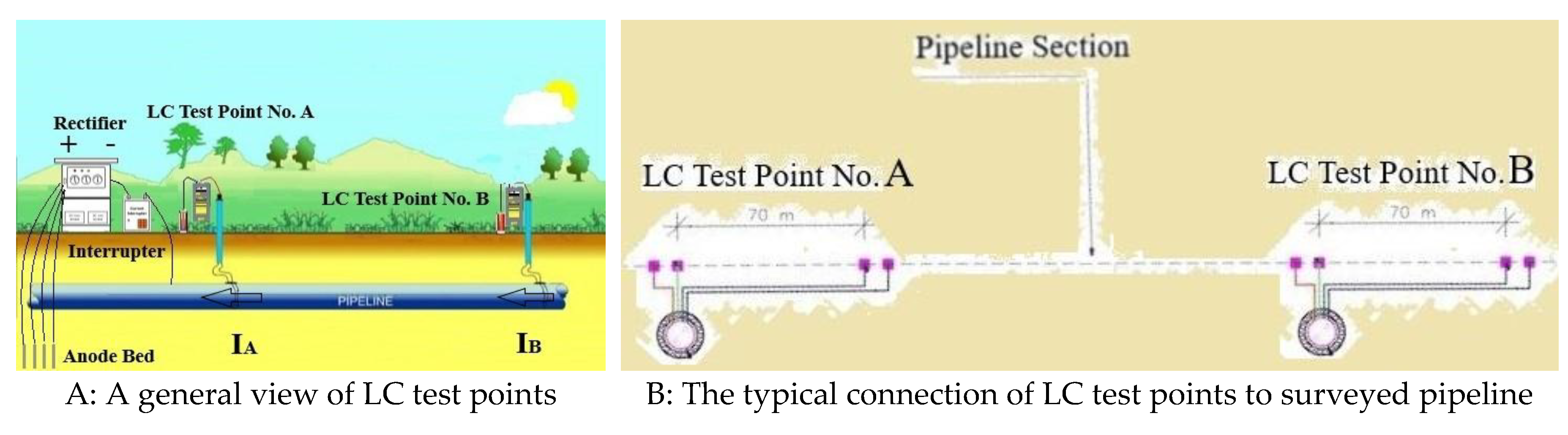
In the LC test points, four copper wires are usually placed in the following configuration: the left pair of wires (LC test point A) is welded to the pipeline at a close distance from each other (typical distance is 15-30 cm). A trench is excavated 50-100 meters away from the first pair of wires, and a second pair of copper wires is installed and connected to the pipeline, as shown in Figure 6. The outward pair is designed to measure electric current, and the inward pair is intended to measure electric voltage, including calibration of the pipeline’s span against the defined length (50-100 meters).
- 4.2.4.
-
The procedure for determining the coating electrical resistance from Line Current attenuation measurements is detailed in the standard [38] and in the reference [88]. Following the review of the LCA procedure principles, which were derived from the two above technical sources, the modified procedure comprises a few stages:
-
1st stage – Calibration of the Line Current (Four Wires) test points for determining the electrical resistance of the tested pipeline sections with defined LC length. The general arrangement for pipeline current measurement calibration is shown in Figure 6. An additional option for calculating the electrical resistance of the tested section is provided by the formula in Appendix B (Standard Pipe Data Tables) of the standard [38] but it is less precise method referred to calibration. The main steps of the section’s calibration are:
- Measuring and recording the initial voltage (U0cal, mV) between inward terminals, as shown in Figure 6. Noting the voltage polarity.
- Applying a test current Ical (mA) between outward test leads.
- Measuring and recording the voltage (mV) change between inward terminals while interruption is applied with the chosen regime, like On : Off = 8:2 seconds, noting the voltage polarity.
- Measuring and recording the difference in current (mA) between the outward terminals.
- Calculating resistance in span (µΩ):
- Steps 3, 4, and 5 are repeated with different electrical currents to verify results, to obtain additional statistical data and to ensure repeatability.
- 2nd stage – the surveyed pipe section is connected to either a temporary or permanent cathodic station with a connected current interrupter at a specific time regime, like On:Off = 8:2 seconds. Measuring, recording, and calculating the potential change (ΔU) at each LC test location (µV or mV) between ON and OFF potentials:
- 3rd stage – calculating the pipe current at each LC test location from the 1st and 2nd stages.
- 4th stage - the surveyed pipe section is still connected to a temporary or permanent cathodic station with a current interrupter, like On:Off = 8:2 seconds. The measurement of the “ON” (φon [mV]) and “Off” (φoff [mV]) structure-to-electrolyte potentials at each LC test location should be conducted, as in the standard [90]. Calculating the difference between ON and OFF potentials.Δ φpipe= φON - φOff
- 5th stage – Measuring the Soil Resistivity near each LC test location according to the Wenner four-pin or Soil-box method [91]. Calculating the average soil resistivity of the surveyed pipeline section.
- 6th stage - calculating the surface area (A) of the surveyed pipe section between LC test locations (m2)where D - pipe outside diameter and L - length of the pipe sectionA=π·D·L
- 7th stage - calculate the average change in pipe-to-electrolyte potential (Δφ avg) for each pipeline section (between LC test points A and B).
- 8th stage - calculating the current pick-up (ΔI) for each pipeline section (between LC test points A and B):∆I=∆IA-∆IB
- 9th stage - finally, calculating the coating average specific electrical resistance (Rcoat) for the pipeline section (between LC test points A and B) in Ω·m2.
- The obtained results have been normalized for a specific soil resistivity of 10 Ω·m according to the requirements of the standard [38].
-
- 4.2.5.
- To determine the aging rate of the polymer-coated underground steel pipelines, several sections of oil/gas (G1-G4) and water pipelines (N1-N4) were selected as shown in Table 1, respectively.
Additional remarks about oil/gas and water pipelines:
The standard steel grade for pipes is X42, with a typical length of 12.2 meters and varying wall thicknesses according to the standard [92].
Standard factory-applied external coating: 3-layer extruded HDPE with varying coating thicknesses according to the standard [45].
The tests for oil/gas pipeline sections were conducted on the straight sections between oil/gas stations, which did not include all the components within the stations, such as epoxy-coated T-connections (T-joints) and elbows. This diminishes the coating’s aging due to potential damage during field application. The absence of T-connections and elbows reduces the risk of premature aging. Pipeline sections with isolation joints at their edges were selected to enable an electrical separation between the inspected pipeline sections and the entire pipeline network. This type of arrangement facilitated the execution of two concurrent inspections: Cathodic Polarization (Drainage Test) and upgraded Line Current Tests.
The characteristics of water pipelines differ significantly from those of gas and oil pipelines. This includes numerous T-connections (T-joints) and elbows with diverse coating types applied under field conditions, primarily two-layer epoxy coatings from various manufacturers. Coating breakdown factors of 2-part epoxy, particularly those applied in the field conditions on T-joints and elbows, are much higher than those of 3LPE factory-applied coating [34,36,51]. This directly contributes to the potential for faster degradation of the pipeline’s overall coating. Locating pipeline sections with isolation joints in water pipelines is challenging, unlike in gas and oil pipelines. As a result, performing a Drainage Test (Cathodic Polarization) to determine the insulation’s condition is not feasible, and only the modified LCA test might be appropriate for that aim.
The following main instruments and auxiliary accessories have been used for the measurements:
Universal measuring instrument with datalogger MiniLog2, Weilekes Elektronik GmbH, Germany
Multimeters: Fluke 187/189/287, Fluke Europe B.V., The Netherlands and Model LC-4.5 Voltmeter, M.C. Miller, USA
Reference Electrode, type RE-5C, Cu/CuSO4, M.C. Miller, USA
Synchronization MicroMax GPS360 Current Interrupter with GPS, American Innovations, USA
Metallic Cables/Leads from various manufacturers and with different section areas.
5. Results and Discussion
- 5.1
- Polyethylene-coated steel pipelines age with time [93,94,95,96]. The polymer coating degrades due to numerous factors [17,18,19,97,98], such as soil composition, static and dynamic stresses, groundwater, microorganisms, and temperature [21,22,23,24]. Aging leads to the formation of spot defects and/or group defects. This may result in loss of the coating’s protective properties, manifested in a decrease in the overall polymer coating resistance [99].
- 5.2
- A decline in the coating’s electrical resistance during the pipeline’s operational period means that the current and number of cathodic stations must be increased, or the insulation in that section must be repaired [27].
- 5.3
- Selected field indirect inspection methods are designed to evaluate the average specific electrical resistance of long polymer-coated buried pipelines, due to the presence of defects at the external 3LPE surface. As the defective exposed area increases with service time, the coating’s electrical resistance decreases, resulting in diminished protective properties.
- 5.4
- The minimum criterion for initial coating average specific electrical resistance was set at 3·106 Ω·m2 , obtained and determined after analysis of DT results from our first study [37].
- 5.5
-
Oil/gas pipelinesTo assess the coating average specific electrical resistance of underground oil/gas pipelines over different service periods, two types of inspections have been performed: LCA and DT. Four oil/gas pipelines from our initial study were selected for this purpose (G1-G4). Each section pair, G1-G2 and G3-G4, was arranged sequentially and connected via an oil/gas station.The oldest of these polymer-coated pipelines was 11 years old. To establish the aging model based on the average specific electrical resistance, evaluations were conducted during 3-4 annual measurements. LCA inspections were performed after 8-9, 10 and 11 years in the underground service. DT measurements were conducted only after 10 years. The results were compared with the initial average specific electrical resistance from the first study [37], and the appropriate model was established based on the initial and aged specific electrical resistance results.
- 5.6
-
Water pipelinesThe LCA method only was used to determine the average specific electrical resistance of coatings on underground water pipelines, as no pipeline sections were electrically separated from the water pipeline network by isolation joints, and thus were not suitable for the execution of DT method. For this purpose, four water pipelines from the first study with various technical characteristics were selected [37]. Like the underground oil/gas pipelines, the maximum age of these pipelines was 11 years. The aging model was based on four time periods of inspections conducted – after construction, and after 9, 10, and 11 years in the underground exposure.
- 5.7
- Table 2 summarizes the average specific electrical resistance results over various service periods of 3LPE-coated oil/gas and water pipelines over time, conducted by the LCA and DT methods.
- 5.8
- The analysis and comparison of the data from the LCA and DT methods for the G1-G2 and G3-G4 oil/gas pipeline sections shows a significant difference between the results of the two techniques. This can be attributed to the fact that the DT method assesses the overall average specific electrical resistance of the coating, including two pipeline sequential sections and the oil/gas station located between the investigated pipeline sections. Many irregular shapes, like T-joints, elbows, and similar, in oil/gas stations are field-applied are protected by epoxy protective coatings. The aging rates of field-applied epoxy coatings, based on coating breakdown factors, are considerably higher than that of factory-applied 3LPE coating [36,51]. At the same time, the LCA method assesses the average specific electrical coating resistance of straight pipeline sections between defined LC test points, without considering oil/gas stations with irregularly shaped epoxy coatings. Thus, the coating aging rates of straight pipeline sections, coated with factory-applied 3LPE and field joint 2LPE coatings only, are much smaller than the epoxy ones. Accordingly, the LCA method’s results are more appropriate to model the aging of the polyethylene coating.
- 5.9
- 5.10
-
From the data obtained using the investigated oil/gas pipeline sections, one can identify the following key patterns and dependencies:
- 5.10.1
- The exponential Arrhenius model demonstrated a high determination fitting coefficient (R2) for predicting the aging of 3LPE-coated steel pipelines.
- 5.10.2
- Aging coefficients were determined and defined with a range from 0.05 to 0.07. Thus, the data suggests that 3LPE-coated pipelines exhibit minimal aging and are expected to have a long service life.
- 5.10.3
- The initial average specific electrical resistance of the coating system is a key factor affecting the aging coefficient. The higher it is, the faster the degradation.
- 5.11
- 5.12
-
Analysis of the data collected from the investigated water pipeline sections reveals the following conclusions:
- 5.12.1
- The predictive model based on the exponential Arrhenius model was shown to estimate the aging of 3LPE-coated steel pipelines, with high determination fitting coefficients.
- 5.12.2
- The aging coefficients fall within the range of 0.07 to 0.09, which exceeds the aging coefficient determined in oil/gas pipelines, suggesting a higher aging rates. However, the aging coefficient range is also low, proposing a relatively long service life.
- 5.12.3
- Coating systems with high initial electrical resistance tend to exhibit higher aging rates.
- 5.12.4
- An LCA-based inspection was conducted on one of the water pipelines intersecting a 400 kV AC high-voltage power lines (HVAC). Unreliable results were obtained, making it inapt for such method. This conclusion is also relevant to oil/gas pipelines.
- 5.13
-
From the above-derived exponential aging phenomena, a general exponential correlation can be proposed for predicting the aging behavior of polyethylene-coated pipelines. The aging model is based on the exponential decay of coating average specific electrical resistance over time (25) and it is analogous to Arrhenius model (13, 14).where:Rc(t) - The average coating electrical resistance after service time t in underground exposure [Ω·m2];Rc(0) - The initial average coating electrical resistance after installation and backfilling (t=0) [Ω·m2];α - the aging rate coefficient [1/year].t – service time [years]
- 5.14
After establishing the exponential aging prediction model (25), Figure 9 shows the predictive average specific electrical resistance of the protective coating up to 50 years in an underground service.
- 5.15
-
Figure 9 points out the following conclusions:
- 5.15.1
- 3LPE-coated buried pipelines used for water and oil/gas exhibit low aging rates.
- 5.15.2
- Coatings that initially have higher average specific electrical resistance are more prone to faster aging than those with lower initial electrical resistance.
- 5.15.3
- For oil/gas pipelines, the aging coefficient α [1/year] changes in the range of 0.05-0.07; for water pipelines, in the range of 0.07-0.09. This indicates that 3LPE external coatings in oil/gas pipelines age more slowly than in water pipelines. The higher aging rates of polymer-coated water pipelines are primarily due to different coating technical characteristics compared to oil/gas pipelines, which contain numerous irregular geometrical connections (T-joints, elbows, consumer connections, air, and drainage points). Most of the connections are coated with epoxy coatings that applied in field conditions, which have significantly higher aging rates (coating breakdown factors) than the 3LPE factory-applied coating [36,51]. For oil/gas pipelines, the polymer-coated pipeline sections are usually constructed without epoxy-coated irregular geometrical shapes and adhere to strict quality control methods and pipeline installation procedures.
- 5.16
- It should be emphasized that some of the results are inaccurate due to the influence of AC-induced voltage; therefore, underground pipelines coated with high-dielectric characteristics and located under parallel or across high-voltage power lines (HVAC: 161 or 400 kV) typically yield unreliable results by LCA testing methods. Hence, the attempt to test the 100-inch diameter water pipeline (N4) resulted in a wide range of results, which were used to establish, albeit ineffectively, the aging coefficients for the prediction model.
- 5.17
- Another source of inaccuracies has been traced to the instrument limits due to the voltage drops in the pipeline, as the measurements are around 1 µV. Hence, sensitive amplifier voltmeters paired with data loggers are necessary. Furthermore, performing several LCA tests is recommended to ensure consistent results. The input impedance of the voltmeters should be at least 10 MΩ.
- 5.18
-
The exponential prediction aging model (25) of the 3LPE coated buried pipelines contradicts the conclusions of the reference [40] and supports the aging model proposed in references [41,42,43], with several significant differences:
- 5.18.1
- The aging coefficient spans across a broader range (0.05 to 0.07 year-1) for oil and gas pipelines, indicating a potentially higher aging rate than the above-cited sources.
- 5.18.2
- Water pipelines exhibit a higher aging rate coefficient range (0.07–0.09 year-1) than oil/gas pipelines. This is primarily attributed to the frequent presence of field irregular-geometry joints, such as T-connections and elbows, where two-part epoxy coatings are often applied in the field.
- 5.18.3
- Epoxy coatings have significantly higher aging rates, based on coating breakdown factors, than 3LPE factory-applied coating [34].
- 5.19
-
Consequently, it is possible to calculate the residual lifetime for each coated pipeline section at any given operational time. In Appendix A, the examples for calculations of water and gas/oil pipelines are given:
- For the water pipeline, based on our first study [37], section N1 (L = 4,920 m; Ø = 16’’, initial average specific electrical resistance is 2.0·106 Ω·m2, the minimum threshold of average electrical resistance for repair or replacement is 3·104 Ω·m2), the selected calculated aging coefficient α is 0.08 year -1, since the operational time of this pipeline section is 10 years the residual life time is 42.3 years.
- For the oil/gas pipeline, according to [37], the section G2 (L= 7,757 m; Ø = 18’, the initial average specific electrical resistance is 10.9·106 Ω·m2, the minimum threshold of average specific electrical resistance for repair or replacement is 3·104 Ω·m2), the selected aging coefficient α = 0.06 year -1, since the operational time of the pipeline section is 10 years, the residual lifetime is 88.2 years.
- 5.20
- It should be noted that the aging rate of protective coatings is usually higher than that of structural materials (steel). Therefore, insulation degradation does not necessarily indicate corrosion or deterioration of the pipe itself.
6. Conclusions
- 6.1
- Following our initial study [37], an aging model for polyethylene-coated underground pipelines was proposed and validated.
- 6.2
- The model was based on the modified Line Current Attenuation test results used for water and oil/gas pipelines following various service periods and technical parameters. The maximum age of the investigated underground pipelines in this study was 11 years.
- 6.3
-
The following main insights have been derived from this study:
- 6.3.1
- The Line Current Attenuation (LCA) method has proven to be an accurate technique for estimating the specific electrical resistances of 3LPE-coated steel pipelines over their service life (besides the cases of AC induced voltage)
- 6.3.2
- An exponential aging model was developed, based on the coating’s average specific electrical resistance for water and oil/gas pipelines.
- 6.3.3
- Increased initial electrical resistances of polyethylene coatings are directly associated with higher aging coefficients and aging rates.
- 6.4
- The study demonstrated that the coating aging rates of 3LPE-coated water pipelines and oil/gas pipelines are comparatively low. Thus, it can be concluded that degradation in the polyethylene coating exceeding the allowable resistance criterion is caused by localized defects rather than overall coating aging [33,34]. As a result, detecting and repairing local sections with the low coating electrical resistance is vital. This can be achieved by utilizing External Corrosion Direct Assessment (ECDA), indirect inspection methods such as Alternating Current Attenuation Survey (Electromagnetic Method) and/or ACVG/DCVG, as well as direct examinations, during which the insulation is inspected in prioritized test pits according to the standards [26,86]. Post Assessment stage should be combined as the final step of the coating’s and steel’s condition assessment [26].
- 6.5
- Precision equipment capable of recording and analyzing of results is essential, especially in oil/gas pipelines where insulation exhibits high dielectric characteristics.
- 6.6
- To establish a reliable method for determining the average specific electrical resistance of 3LPE-coated buried pipelines under the influence of high-voltage AC power lines (HVAC), further research is required.
Author Contributions
Conceptualization, all authors; methodology, all authors; validation, all authors; formal analysis, all authors; investigation, all authors; writing—original draft preparation, G.R.N.; writing—review and editing, all authors; visualization, G.R.N. supervision, S.K, K.K.; project administration, G.R.N.; funding acquisition, G.R.N. All authors have read and agreed to the published version of the manuscript.
Funding
Some of the tests were funded by Mekorot – Israeli National Water Co.
Data Availability Statement
The data presented in this study are available on request from the corresponding author.
Conflicts of Interest
The author G. R. Neizvestny was employed by Mekorot – Israeli National Water Co. The remaining authors declare that the research was conducted in the absence of any commercial or financial relationships that could be construed as a potential conflict of interest.
Appendix A. Examples of the Residual Isolation Lifetime Calculations for Oil/Gas and Water Pipelines
- The calculation for water pipeline section N1
The general formula for predicting the aging behavior of coating average specific electrical resistance over time (for N1 water pipeline section) is:
RC(t)=2.0·106e-0.080t
After 10 years of service, the coating average specific electrical resistance, Rc(10) will be:
RC(t)=2.0·106e-0.080·10=8.8·105 Ω·m2
The calibrated line current passed at the starting point is 922.25 mA, and at the end LC point, it is 917.77 mA. The difference between them is ΔI=4.48 mA.
The formula for calculating the pipeline section area is A=π·D·L ⤇ , A=6,273 m2.
The current density calculation (after 10 years): j= ΔI/A = 4.48/6,273 = 0.71 µA/m2. The current density measured on coated pipelines after a decade is better than the standard’s recommended range of 1 to 20 µA/m2 for optimized designs, as indicated in Table 3 [38].
The initial current density (0 years): 0.58 µA/m2 (from Drainage Test results).
Specific ratio of coating defects: For average coating electrical resistance of 8.8·105 Ω·m2, the coating condition is good with the range of specific area ratio of coating defects - 0.01÷1.50 mm2/m2 and Defect Size Classification: several very small (IR<1), minor (1≤%IR<3) or single moderate defects (3≤IR<15) [37].
The expected whole lifetime of the protective coating until overall repair:
t= 52.5 years
The expected remaining duration of the protective coating until overall repair is:
52.5 – 10 = 42.5 years.
- The calculation for oil/gas pipeline section G2
The general formula for predicting the aging behavior of coating average specific electrical resistance over time (for G2 oil/gas pipeline section) is:
RC(t)=10.9·106e-0.060t
After 10 years of service, the average specific electrical resistance Rc(10) will be:
RC(t)=10.9·106e-0.060·10=6.0·106 Ω·m2
The calibrated line current passed at the starting point is 3.45 mA; at the end, the LC point is zero mA (isolation joint). The difference between them is ΔI=3.45 mA.
The formula for calculating the pipeline section area is A=π·D·L ⤇ A=11,136 m2.
The current density calculation (after 10 years): j= is ΔI/A = 3.45/11,136 = 0.31 µA/m2. The measured current density for coated pipelines after 10 years is much better than the standard’s recommended range of 1 to 20 µA/m2 for optimized designs, as shown in Table [38].
The initial current density (0 years): 0.07 µA/m2 (from Drainage Test results).
Specific ratio of coating defects: For coating average specific electrical resistance of 6.0·106 Ω·m2, the coating condition is excellent with the range of specific area ratio of coating defects below 0.01 mm2/m2 and defect size classification: minimal single defects (IR<1) [37].
The expected whole lifetime of the protective coating until repair:
t= 98.2 years, and the residual lifetime is 88.2 years
References
- Gas Transmission Miles By Decade Installed, Data Source: US DOT Pipeline and Hazardous Materials Safety Administration, 2025, (n.d.).
- Fact Sheet - Corrosion, U.S. Department of Transportation, Pipeline and Hazardous Materials Safety Administration, Washington DC, https://primis.phmsa.dot.gov/comm/FactSheets/FSCorrosion.htm?nocache=9090, (n.d.).
- Gas Pipeline Incidents, 12th Report of the European Gas Pipeline Incident Data Group (period 1970 – 2022) , December 2023, European Gas Pipeline Incident Data Group (EGIG), https://www.EGIG.eu, (n.d.).
- A.E. Romer, G.E.C. A.E. Romer, G.E.C. Bell, Causes of External Corrosion on Buried Water Mains, in: Pipelines 2001, American Society of Civil Engineers, San Diego, California, United States, 2001: pp. 1–9. [CrossRef]
- ASME B31.8 - 2022: Gas Transmission and Distribution Piping Systems, ASME Code for Pressure Piping, B31, December 2022, The American Society of Mechanical Engineers, New York, NY, USA, (n.d.).
- American Water Works Association, Prestressed Concrete Pressure Pipe, Steel-Cylinder Type, (2007). [CrossRef]
- AWWA M11 - Steel Water Pipe: A guide for design and installation, Fifth edition, American Water Works Association, Denver, CO, 2017.
- H. A. Kishawy, H.A. Gabbar, Review of pipeline integrity management practices. International Journal of Pressure Vessels and Piping 2010, 87, 373–380. [Google Scholar] [CrossRef]
- AWWA C213-22 Fusion-Bonded Epoxy Coatings and Linings for Steel Water Pipe and Fittings, (n.d.).
- API RP572-2016 Inspection Practices for Pressure Vessels, 4th Edition, 2016, The American Petroleum Institute (API), (n.d.).
- API RP574-2016, Inspection Practices for Piping System Components, 4th Edition, 2016, The American Petroleum Institute (API), (n.d.).
- ANSI - AWWA C213-15, (n.d.).
- ASME B31.8S 2022 - Managing System Integrity of Gas Pipelines, January 2023, ASME Code for Pressure Piping, B31 Supplement to ASME B31.8, The American Society of Mechanical Engineers, New York, NY, USA, (n.d.).
- H. Zargarnezhad, E. Asselin, D. Wong, C.N.C. Lam, A Critical Review of the Time-Dependent Performance of Polymeric Pipeline Coatings: Focus on Hydration of Epoxy-Based Coatings. Polymers 2021, 13, 1517. [Google Scholar] [CrossRef]
- S. B. Lyon, R. Bingham, D.J. Mills, Advances in corrosion protection by organic coatings: What we know and what we would like to know. Progress in Organic Coatings 2017, 102, 2–7. [Google Scholar] [CrossRef]
- M. Wasim, S. Shoaib, N.M. Mubarak, Inamuddin, A.M. Asiri, Factors influencing corrosion of metal pipes in soils. Environ Chem Lett 2018, 16, 861–879. [Google Scholar] [CrossRef]
- C. Argent, D. C. Argent, D. Norman, Three Layer Polyolefin Coatings: Fulfilling Their Potential?, NACE 61st Annual Conference & Exposition (n.d.). [CrossRef]
- Fletcher, D. Nicholas, Fusion Bonded Polyethylene Coatings – 40 Years On, Paper 094, Corrosion & Prevention 2014 (n.d.).
- B.T.A. Chang, H.-J. B.T.A. Chang, H.-J. Sue, H. Jiang, B. Browning, D. Wong, H. Pham, S. Guo, A. Kehr, M. Mallozzi, W. Snider, A. Siegmund, Integrity of 3LPE Pipeline Coatings: Residual Stresses and Adhesion Degradation, in: 2008 7th International Pipeline Conference, Volume 2, ASMEDC, Calgary, Alberta, Canada, 2008: pp. 75–86. [CrossRef]
- H. M.H. Farh, M.E.A. Ben Seghier, T. Zayed, A comprehensive review of corrosion protection and control techniques for metallic pipelines. Engineering Failure Analysis 2023, 143, 106885. [Google Scholar] [CrossRef]
- N. Guermazi, K. Elleuch, H.F. Ayedi, Ph. Kapsa, Aging effect on thermal, mechanical and tribological behaviour of polymeric coatings used for pipeline application. Journal of Materials Processing Technology 2008, 203, 404–410. [Google Scholar] [CrossRef]
- D. Melot, G. D. Melot, G. Paugam, M. Roche, Disbondments of Pipeline Coatings and their effects on corrosion risks, 17th International Conference on Pipeline Protection, BHR Group, Edinburgh, 2009, 2007,.
- M. Roche, D. M. Roche, D. Melot, G. Paugam, Recent Experience with Pipeline Coating Failures, 16th International Conference on Pipeline Protection, BHR Group, Paphos, 2005, (n.d.).
- S. Ranade, M.Y. S. Ranade, M.Y. Tan, M. Forsyth, The Effects of Mechanical Stress, Environment and Cathodic Protection on the Degradation and Failure of Coatings: An Overview, Corrosion & Prevention 2014 Paper 50 (n.d.).
- NACE SP0169-2013 Control of External Corrosion on Underground or Submerged Metallic Piping Systems, 2013, NACE International, Houston, Texas, USA, AMPP, 2024. [CrossRef]
- ANSI/NACE SP0502-2010, Pipeline External Corrosion Direct Assessment Methodology, 2010, NACE International, ISBN 1-57590-156-0, AMPP, 2010. [CrossRef]
- AWWA M28 Rehabilitation of water mains, Manual of Water Supply Practices — M28, Third Edition Rehabilitation of Water Mains, 2014, American Water Works Association (AWWA), Denver, USA, awwa.org, (n.d.).
- R. Morrison, T. R. Morrison, T. Sangster, D. Downey, J. Matthews, W. Condit, S. Sinha, S. Maniar, R. Sterling, State of Technology for Rehabilitation of Water Distribution Systems, National Risk Management Research Laboratory Office of Research and Development U.S. Environmental Protection Agency, Ohio, USA (2013) www.epa.gov/gateway/science.
- D. S. De Freitas, S.L.D.C. Brasil, G. Leoni, G.X.D. Motta, E.G.B. Leite, J.F.P. Coelho, Long--term cathodic disbondment tests in three--layer polyethylene coatings. Materials & Corrosion 2023, 74, 1159–1168. [Google Scholar] [CrossRef]
- Bobbi Jo Merten, Coating Evaluation by Electrochemical Impedance Spectroscopy (EIS), Research and Development Office Science and Technology Program Final Report ST-2016-7673-1, December 2015, Research and Development Office U.S. Department of the Interior, Bureau of Reclamation, Denver CO USA, (n.d.).
- B.J.E. Merten, Electrochemical Impedance Methods to Assess Coatings for Corrosion Protection, Technical Publication No. 8540-2019-03 U.S. Department of the Interior Bureau of Reclamation Technical Service Center Materials and Corrosion Laboratory Denver, Colorado, USA (2019).
- D. J. Mills, S.S. Jamali, The best tests for anti-corrosive paints. And why: A personal viewpoint. Progress in Organic Coatings 2017, 102, 8–17. [Google Scholar] [CrossRef]
- EN 12954-2019, General principles of cathodic protection of buried or immersed onshore metallic structures, 2019, EUROPEAN COMMITTEE FOR STANDARDIZATION, Brussels, (n.d.).
- ISO_15589-1 - 2015 (en), Petroleum, petrochemical and natural gas industries — Cathodic protection of pipeline systems Part 1: On-land pipelines, 2015, Geneva, Switzerland, (n.d.).
- DNV RP B401 - 2021, Cathodic Protection Design, 2021, DNV AS, Oslo, Norway, (n.d.).
- DNVGL-RP-F103-2016, Cathodic protection of submarine pipelines, 2016, DNV GL AS, Oslo, Norway, (n.d.).
- G. Neizvestny, S. Kenig, and K. Kovler, Comprehensive Methodology for Quality Assurance Following Installation and Backfilling of Polymer-Coated Steel Pipelines, Draft, Under Revision, October 2025, (n.d.).
- AMPP (NACE) TM0102-23: Measurement of Protective Coating Electrical Conductance on Underground Pipelines, ©2023 Association for Materials Protection and Performance (AMPP) (n.d.). [CrossRef]
- GOST R 51164-1998, General Requirements for Protection against Corrosion, 1998, Gosstandard of Russia, Moscow, (n.d.).
- W. von Baeckmann, W. W. von Baeckmann, W. Schwenk, W. Prinz, eds., Handbook of cathodic corrosion protection: theory and practice of electrochemical protection processes, 3rd ed, Gulf Pub. Co, Houston, Tex, 1997.
- N. P. Glazov, K.L. Shamshetdinov, Protection of Steel Pipelines against Underground Corrosion. Protection of Metals 2002, 38, 172–175. [Google Scholar] [CrossRef]
- N. P. Glazov, Peculiarities of the Corrosion Protection of Steel Underground Pipelines. Protection of Metals 2004, 40, 468–473. [Google Scholar] [CrossRef]
- N. P. Glazov, K.L. Shamshetdinov, N.N. Glazov, Comparative analysis of requirements to insulating coatings of pipelines. Prot Met 2006, 42, 94–99. [Google Scholar] [CrossRef]
- ISO 21809-1:2018 Petroleum and natural gas industries — External coatings for buried or submerged pipelines used in pipeline transportation systems Part 1: Polyolefin coatings (3-layer PE and 3-layer PP), 2018, Geneva, Switzerland, (n.d.).
- DIN 30670-2012, Polyethylene coatings on steel pipes and fittings Requirements and testing, 2012, DIN Deutsches Institut für Normung, Berlin, Germany, (n.d.).
- American Water Works Association, ANSI/AWWA C215-10, Extruded Polyolefin Coatings for the Exterior of Steel Water Pipelines, (2010). [CrossRef]
- SI 30670-2021, Polyethylene coatings on steel pipes and fittings – Requirements and testing (Updates in Hebrew), 2021, SII, Tel Aviv, Israel, (n.d.).
- ISO 21809-3: 2016, Petroleum and natural gas industries — External coatings for buried or submerged pipelines used in pipeline transportation systems Part 3: Field joint coatings, 2016, Geneva, Switzerland, (n.d.).
- DIN 30672-2000, Tape and shrinkable materials for the corrosion protection of buried or underwater pipelines without cathodic protection for use at operating temperatures up to 50 °C, 2000, DIN Deutsches Institut für Normung and DVGW Deutscher Verein des Gas-und Wasserfaches e.V. (German Associaton of Gas and Water Engineers), Berlin, Germany, (n.d.).
- BS EN 12068:1999, Cathodic protection. External organic coatings for the corrosion protection of buried or immersed steel pipelines used in conjunction with cathodic protection. Tapes and shrinkable materials, ISBN: 0580302296, British Standards Institution, London, 1999.
- DNV-RP-F102: Pipeline Field Joint Coating and Field Repair of Linepipe Coating, (2011).
- Steve Lampman, Characterization and Failure Analysis of Plastics, Copyright © 2003 by ASM International, pp. 28-48,. [CrossRef]
- L. McKeen, The effect of heat aging on the properties of polyolefins, polyvinyls, and acrylics, in: The Effect of Long Term Thermal Exposure on Plastics and Elastomers, Elsevier, 2021: pp. 177–202. [CrossRef]
- P. Gijsman, Review on the thermo-oxidative degradation of polymers during processing and in service. E-Polymers 2008, 8. [Google Scholar] [CrossRef]
- D. Feldman, Polymer Weathering: Photo-Oxidation, Journal of Polymers and the Environment, Vol. 10, No. 4, October 2002 (n.d.).
- J. R. White, A. Turnbull, Weathering of polymers: mechanisms of degradation and stabilization, testing strategies and modelling. Journal of Materials Science 1994, 29, 584–613. [Google Scholar] [CrossRef]
- Hsuan, Y.G. , Koerner, R.M., Antioxidant depletion lifetime in high density polyethylene geomembranes, Journal of Geotechnical and Geoenvironmental Engineering ASCE, 532–541, 1998., (n.d.).
- R. K. Rowe, H.P. Sangam, Durability of HDPE geomembranes. Geotextiles and Geomembranes 2002, 20, 77–95. [Google Scholar] [CrossRef]
- W.L. Hawkins, Polymer Degradation and Stabilization, Springer Berlin Heidelberg, Berlin, Heidelberg, 1984. [CrossRef]
- Plota, A. Masek, Lifetime Prediction Methods for Degradable Polymeric Materials—A Short Review. Materials 2020, 13, 4507. [Google Scholar] [CrossRef]
- H. P. Sangam, R.K. Rowe, Effects of exposure conditions on the depletion of antioxidants from high-density polyethylene (HDPE) geomembranes. Can. Geotech. J. 2002, 39, 1221–1230. [Google Scholar] [CrossRef]
- R. K. Rowe, M.Z. Islam, R.W.I. Brachman, D.N. Arnepalli, A.R. Ewais, Antioxidant Depletion from a High Density Polyethylene Geomembrane under Simulated Landfill Conditions. J. Geotech. Geoenviron. Eng. 2010, 136, 930–939. [Google Scholar] [CrossRef]
- Norman Grassie & Gerald Scott, Polymer Degradation and Stabilisation, Cambridge University Press, Cambridge, 1985, (n.d.).
- F. Gugumus, Critical antioxidant concentrations in polymer oxidation—I. Fundamental aspects. Polymer Degradation and Stability 1998, 60, 85–97. [Google Scholar] [CrossRef]
- Y.G. Hsuan, H.F. Y.G. Hsuan, H.F. Schroeder, K. Rowe, W. Müller, J. Greenwood, D. Cazzuffi, R.M. Koerner, Long-term Performance and Lifetime Prediction of Geosynthetics, (n.d.).
- Gerald Scott, Antioxidants, Bull. Chem. Soc. Jpn., 61, 165- 1988, 170, The Chemical Society of Japan, (n.
- H. Zweifel, Stabilization of Polymeric Materials, Springer Berlin Heidelberg, Berlin, Heidelberg, 1998. [CrossRef]
- G., Pritchard (Ed.) G. Pritchard, ed., Plastics Additives: An A-Z reference (pp. 73-79), Springer Netherlands, Dordrecht, 1998. [CrossRef]
- Y. Hsuan, R. Y. Hsuan, R. Koerner, A. Lord, A Review of the Degradation of Geosynthetic Reinforcing Materials and Various Polymer Stabilization Methods, in: Geosynthetic Soil Reinforcement Testing Procedures, ASTM International100 Barr Harbor Drive, PO Box C700, West Conshohocken, PA 19428-2959, 1993: pp. 228–243. [CrossRef]
- P. P. Klemchuk, P.-L. Horng, Transformation products of hindered phenolic antioxidants and colour development in polyolefins. Polymer Degradation and Stability 1991, 34, 333–346. [Google Scholar] [CrossRef]
- W. D. Habicher, I. Bauer, J. Pospíšil, Organic Phosphites as Polymer Stabilizers. Macromolecular Symposia 2005, 225, 147–164. [Google Scholar] [CrossRef]
- K. J. Humphris, G. Scott, Mechanisms of antioxidant action: reactions of phosphites with hydroperoxides. J. Chem. Soc., Perkin Trans. 1973, 2, 826. [Google Scholar] [CrossRef]
- R. P. Krushelnitzky, R.W.I. Brachman, Antioxidant depletion in high-density polyethylene pipes exposed to synthetic leachate and air. Geosynthetics International 2011, 18, 63–73. [Google Scholar] [CrossRef]
- Y.G. Hsuan, M. Y.G. Hsuan, M. Li, R.M. Koerner, Stage “‘C’” Lifetime Prediction of HDPE Geomembrane Using Acceleration Tests with Elevated Temperature, in: Geosynthetics Research and Development in Progress, American Society of Civil Engineers, Austin, Texas, United States, 2008: pp. 1–5. [CrossRef]
- W. W. Müller, I. Jakob, R. Tatzky-Gerth, A. Wöhlecke, A study on antioxidant depletion and degradation in polyolefin-based geosynthetics: Sacrificial versus regenerative stabilization. Polym Eng Sci 2016, 56, 129–142. [Google Scholar] [CrossRef]
- Y.G. Hsuan, H.F. Y.G. Hsuan, H.F. Schroeder, K. Rowe, W. Müller, J. Greenwood, D. Cazzuffi, R.M. Koerner, Long-term Performance and Lifetime Prediction of Geosynthetics, EuroGeo4 Keynote Paper, 2016 (n.d.).
- R. M. Koerner, A.E. Lord, Y.H. Hsuan, Arrhenius modeling to predict geosynthetic degradation. Geotextiles and Geomembranes 1992, 11, 151–183. [Google Scholar] [CrossRef]
- A.S. Maxwell, W.R. A.S. Maxwell, W.R. Broughton, G. Dean, G.D. Sims, Review of accelerated ageing methods and lifetime prediction techniques for polymeric materials, NPL Report DEPC MPR 016, National Physical Laboratory, UK (2005).
- R.L. Feller, Accelerated aging: photochemical and thermal aspects, Getty Conservation Institute, Marina del Rey, CA, 1994.
- S. Maxwell and W. R. Broughton, NPL Report MAT 85, Survey of long-term durability testing of composites, adhesives and polymers, National Physical Laboratory, NPL Management Limited, 2017, (n.d.).
- R. M. Koerner, G. R. R. M. Koerner, G. R. Koerner, Y. Hsuan and W. K. Wong, GRI Report #42 - Lifetime Prediction of Laboratory UV Exposed Geomembranes- Part I- Using A Correlation Factor, Geosynthetic Institute, USA, 2012, (n.d.).
- R. Bonaparte, D. E. R. Bonaparte, D. E. Daniel, R. M. Koerner, Assessment and Recommendations for Improving the Performance of Waste Containment Systems, EPA/600/R-02/099, 2002, (n.d.).
- A.J. Doheny, SERVICE LIFETIME OF POLYOLEFIN-BASED PIPELINE COATINGS BY ACCELERATED TESTING OF THERMAL STABILITY, Paper No. 610, NACE International, 1998 (n.d.).
- DVWG GW 12 (A) 2010, Technische Regel – Arbeitsblatt, Planung und Einrichtung des kathodischen Korrosionsschutzes (KKS) für erdverlegte Lagerbehälter und Stahlrohrleitung ((Planning and installing of cathodic corrosion protection (CP) for buried storage tanks and steel pipes - p. 7.2), Bonn, Germany, (n.d.).
- AfK-Empfehlung, Nr. 10 - 2000, Verfahren zum Nachweis der Wirksamkeit des des kathodischen Korrosionsschutzes an erdverlegten Rohrleitungen; DVGW, Bonn, Germany, (n.d.).
- NACE TM0109-09, Aboveground survey techniques for the evaluation of underground coating condition, 2009, NACE International, ISBN 1-57590-226-5, (n.d.).
- NACE SP0207-2007, Performing close-interval potential surveys and DC surface potential gradient surveys on buried or submerged metallic pipelines, NACE International, Houston, Tex., 2007.
- W.B. Holtsbaum, Cathodic protection survey procedures, NACE International, Houston, Tex, 2009.
- NACE SP0286-2007, Standard recommended practice: electrical isolation of cathodically protected pipelines, NACE International, Houston, TX, 2007.
- NACE Standard TM0497-2012, Standard Test Method, Measurement Techniques Related to Criteria for Cathodic Protection on Underground or Submerged Metallic Piping Systems, NACE International, Houston, TX, USA, AMPP, 2022. [CrossRef]
- ASTM G57 - Standard Test Method for Field Measurement of Soil Resistivity Using the Wenner Four-Electrode Method, ASTM, USA, (n.d.).
- ANSI/API 5L, ISO 3183:2007 (Modified), Petroleum and natural gas industries – Steel pipe for pipeline transportation systems, 44th Edition, 2007, American Petrolium Institute, the International Organization for Standardization, (n.d.).
- L. I. Nyrkova, S.O. Osadchuk, L.V. Goncharenko, A.O. Rybakov, Yu.O. Kharchenko, Influence of long-term operation on the properties of main gas pipeline steels. A review. Phys. Chem. Sol. State 2024, 25, 191–202. [Google Scholar] [CrossRef]
- S. A. Shipilov, I. Le May, Structural integrity of aging buried pipelines having cathodic protection. Engineering Failure Analysis 2006, 13, 1159–1176. [Google Scholar] [CrossRef]
- B. Y. Fang, A. Atrens, J.Q. Wang, E.H. Han, Z.Y. Zhu, W. Ke, Review of stress corrosion cracking of pipeline steels in “low” and “high” pH solutions. Journal of Materials Science 2003, 38, 127–132. [Google Scholar] [CrossRef]
- F. Hasan, J. Iqbal, F. Ahmed, Stress corrosion failure of high-pressure gas pipeline. Engineering Failure Analysis 2007, 14, 801–809. [Google Scholar] [CrossRef]
- D. S. De Freitas, S.L.D.C. Brasil, G. Leoni, G.X.D. Motta, E.G.B. Leite, J.F.P. Coelho, Long--term cathodic disbondment tests in three--layer polyethylene coatings. Materials & Corrosion 2023, 74, 1159–1168. [Google Scholar] [CrossRef]
- M. Y. Tan, F. Varela, Y. Huo, R. Gupta, D. Abreu, F. Mahdavi, B. Hinton, M. Forsyth, An Overview of New Progresses in Understanding Pipeline Corrosion. Corrosion Science and Technology 2016, 15, 271–280. [Google Scholar] [CrossRef]
- A.W. Peabody, Peabody’s Control of Pipeline Corrosion, 3rd ed., NACE International, The Worldwide Corrosion Authority15835 Park Ten Place, Houston, TX 77084, 2018. [CrossRef]
Figure 1.
Three fundamental stages (A-C) describing the chemical degradation process of HDPE geomembranes [58,63].
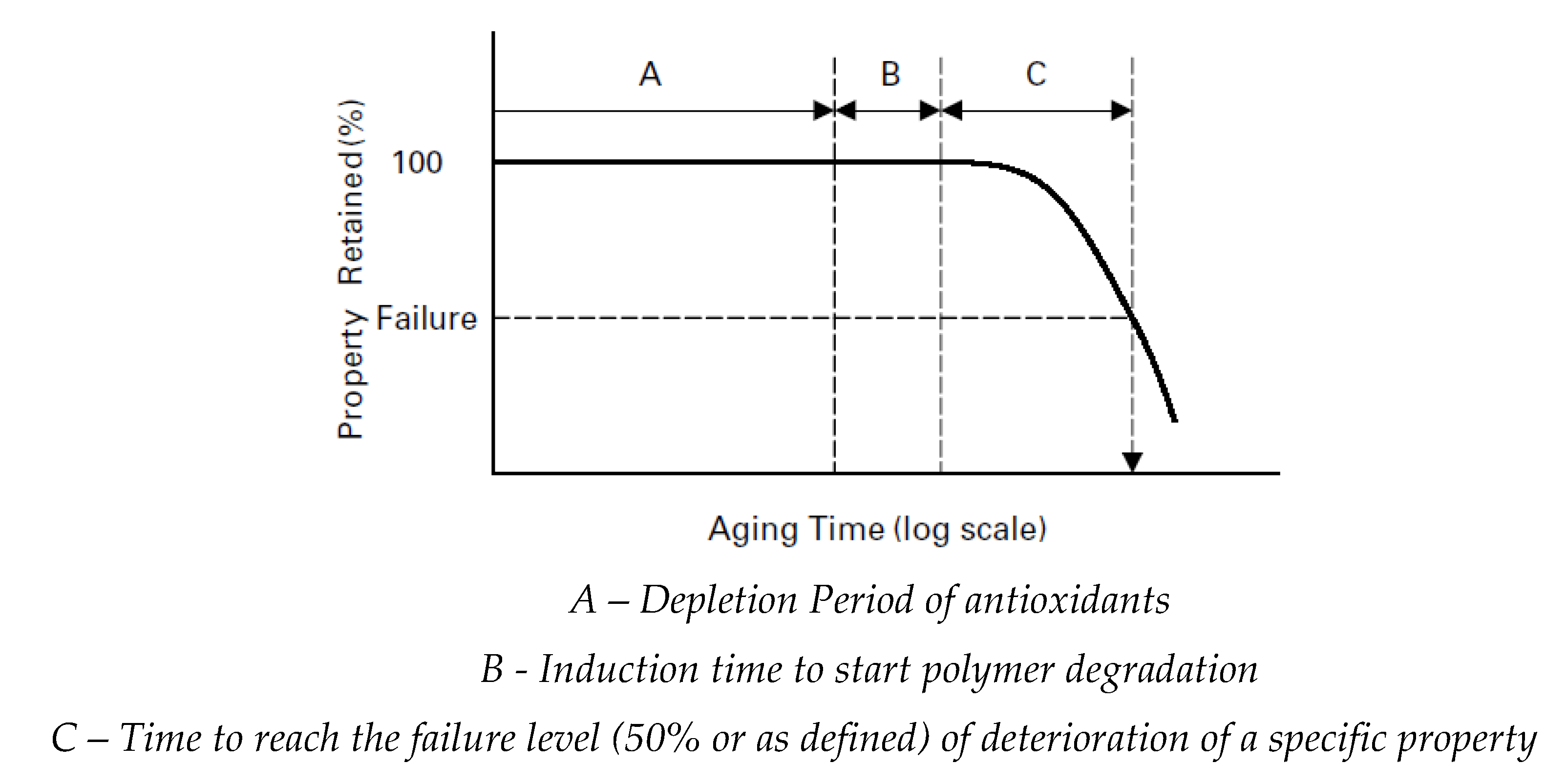
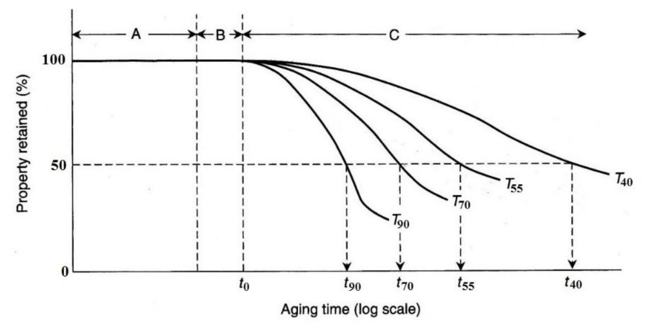
Figure 3.
Schematic Arrhenius plot for data analysis and extrapolation of reaction rate at the temperature of a specific site (1/(273+Tsite) [81,82].
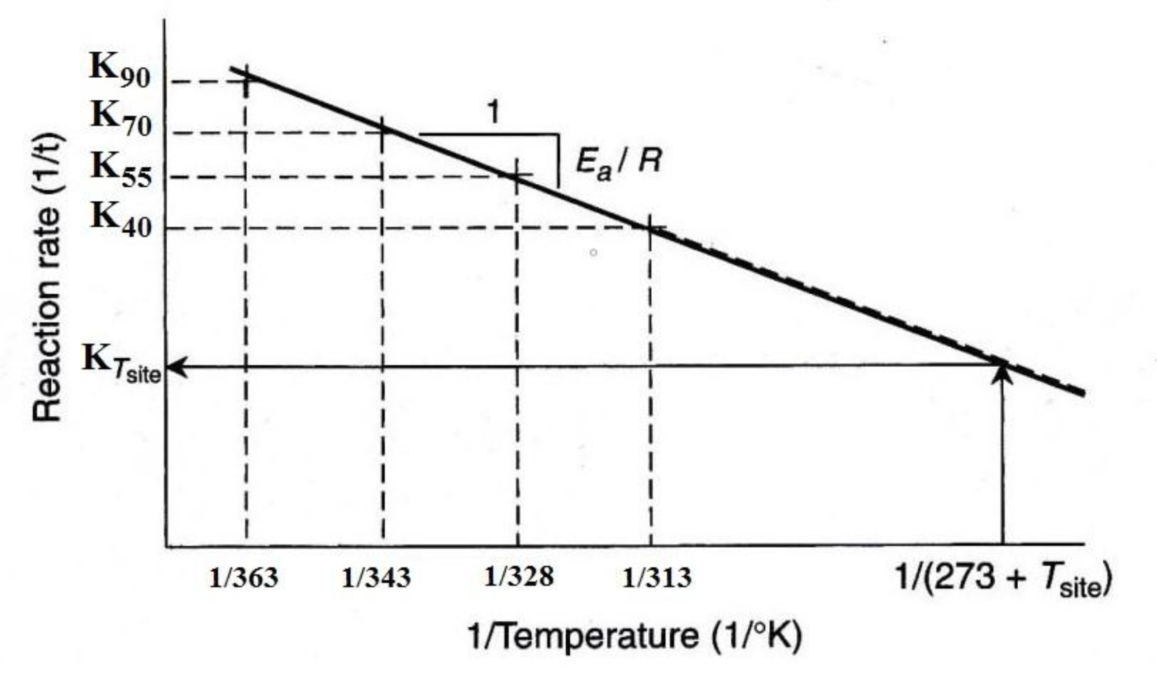
Figure 4.
Schematics of the drainage test setup.
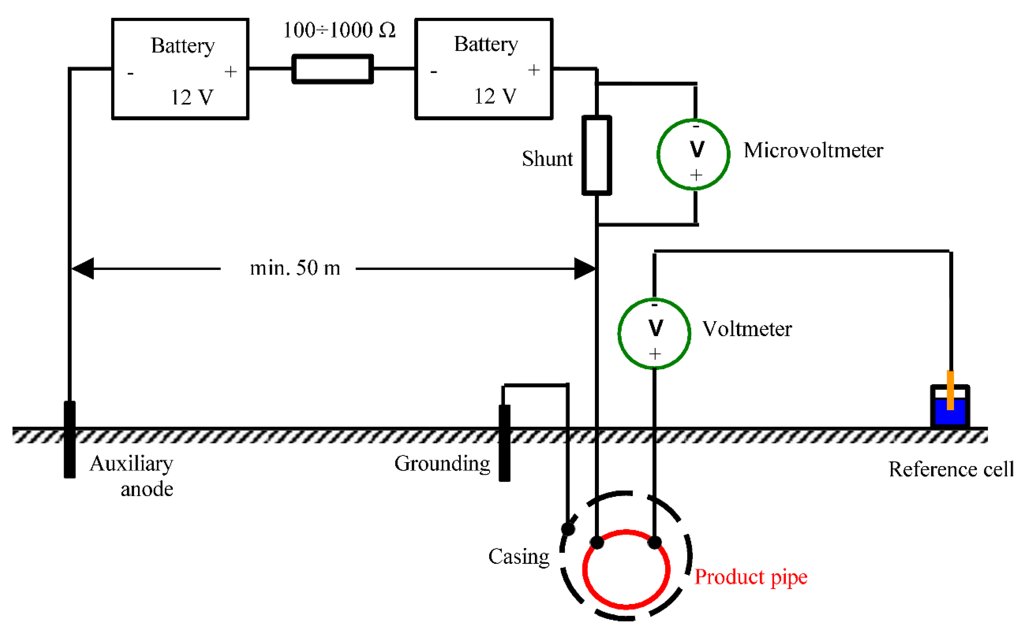
Figure 6.
LC Test point Configuration for Calibration of pipeline span (four wires).
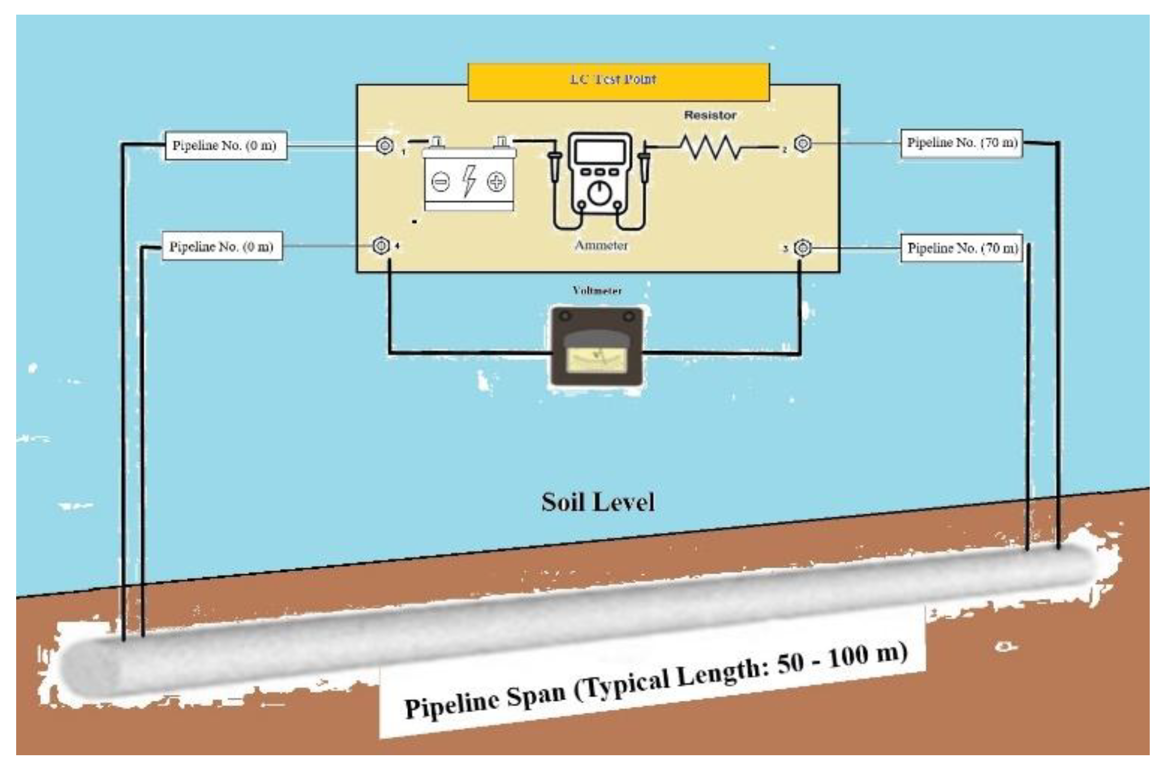
Figure 7.
Aging exponential model based on average specific electrical coating resistance for G1, G2, G3, and G4 oil/gas pipeline sections based on LCA method.
Figure 7.
Aging exponential model based on average specific electrical coating resistance for G1, G2, G3, and G4 oil/gas pipeline sections based on LCA method.
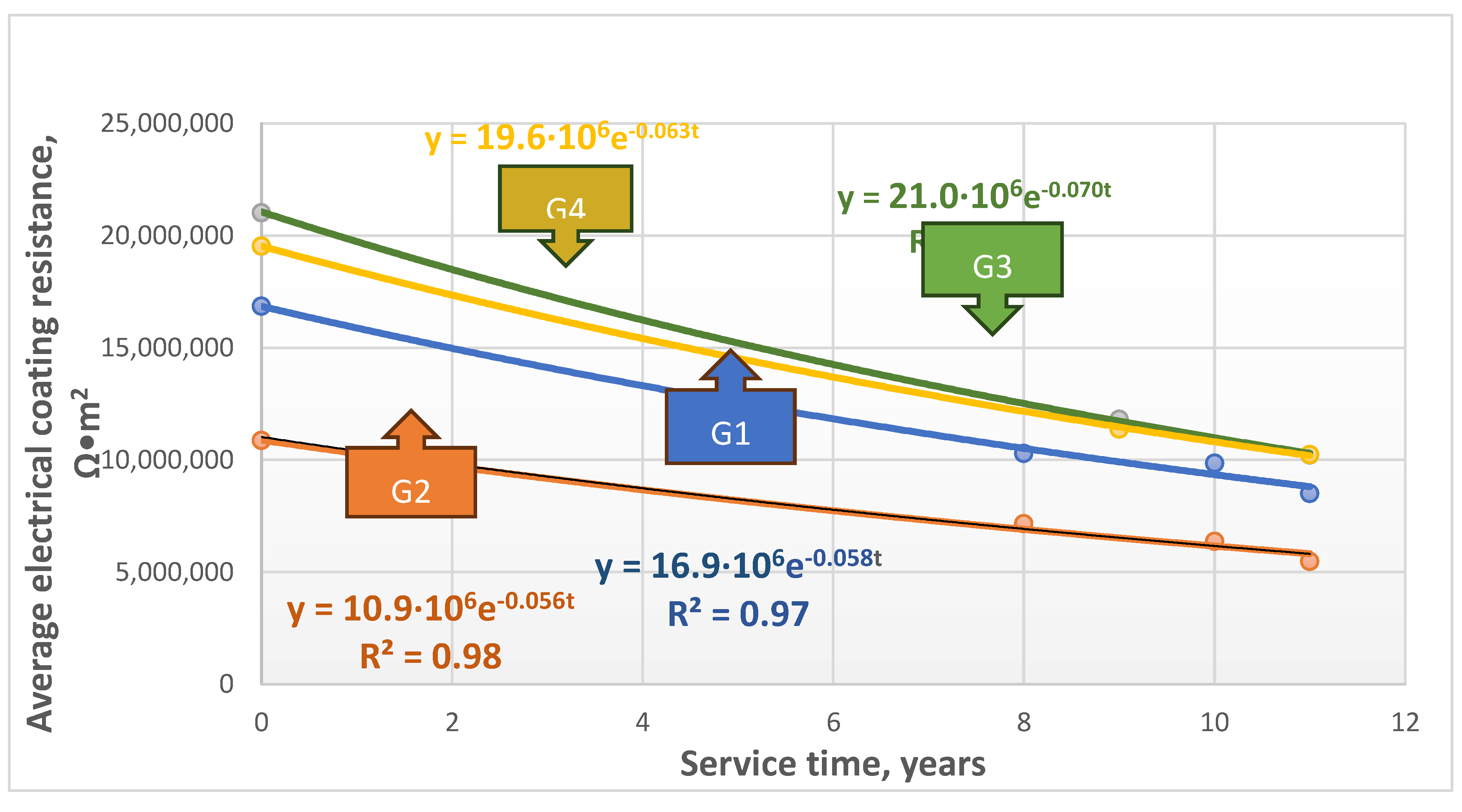
Figure 8.
Aging exponential model based on average specific electrical coating resistance for N1, N2, and N3 water pipelines.
Figure 8.
Aging exponential model based on average specific electrical coating resistance for N1, N2, and N3 water pipelines.
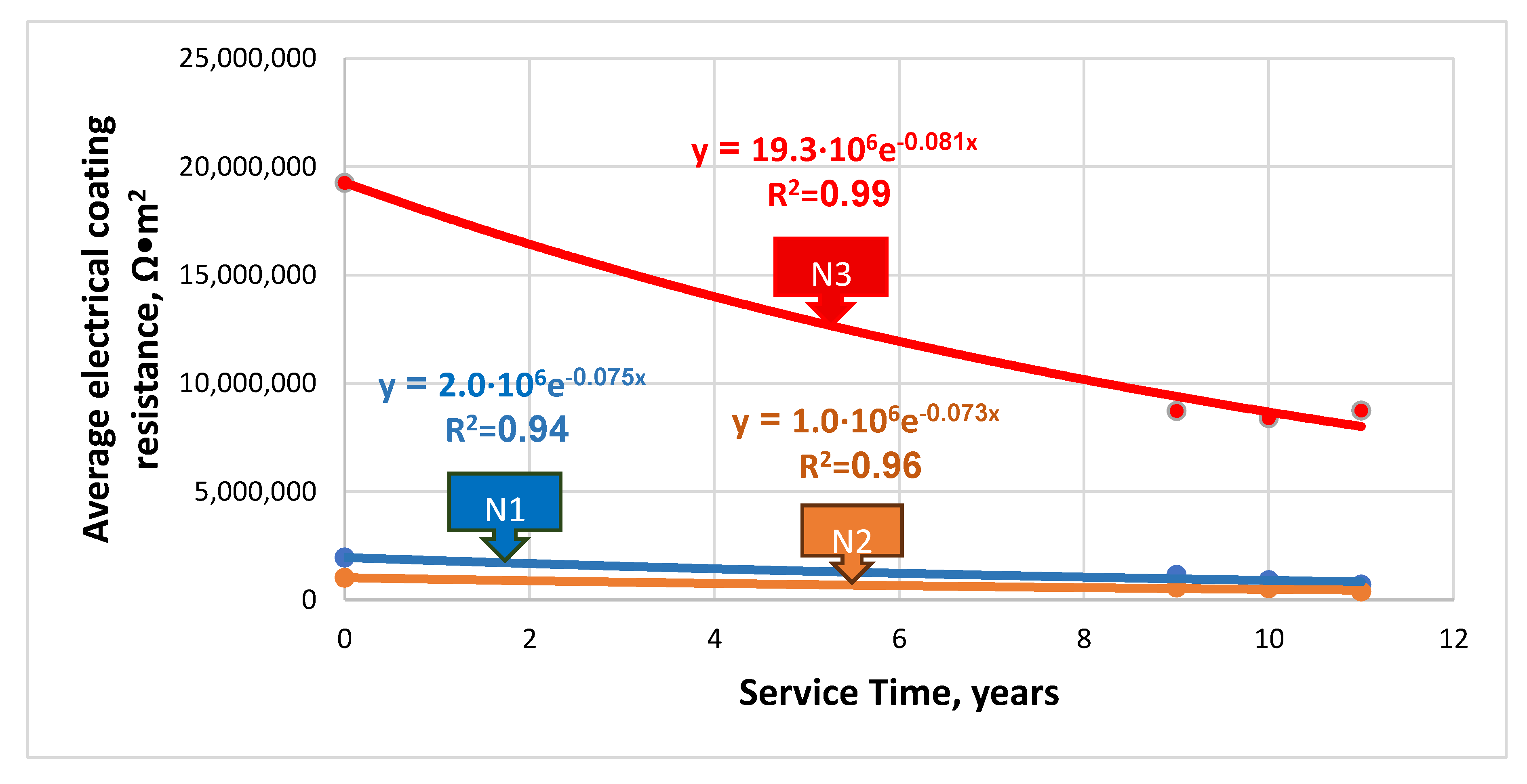
Figure 9.
Aging prediction model of coating average specific electrical resistances (Ω•m2) for oil/gas and water pipelines with different aging coefficients.
Figure 9.
Aging prediction model of coating average specific electrical resistances (Ω•m2) for oil/gas and water pipelines with different aging coefficients.
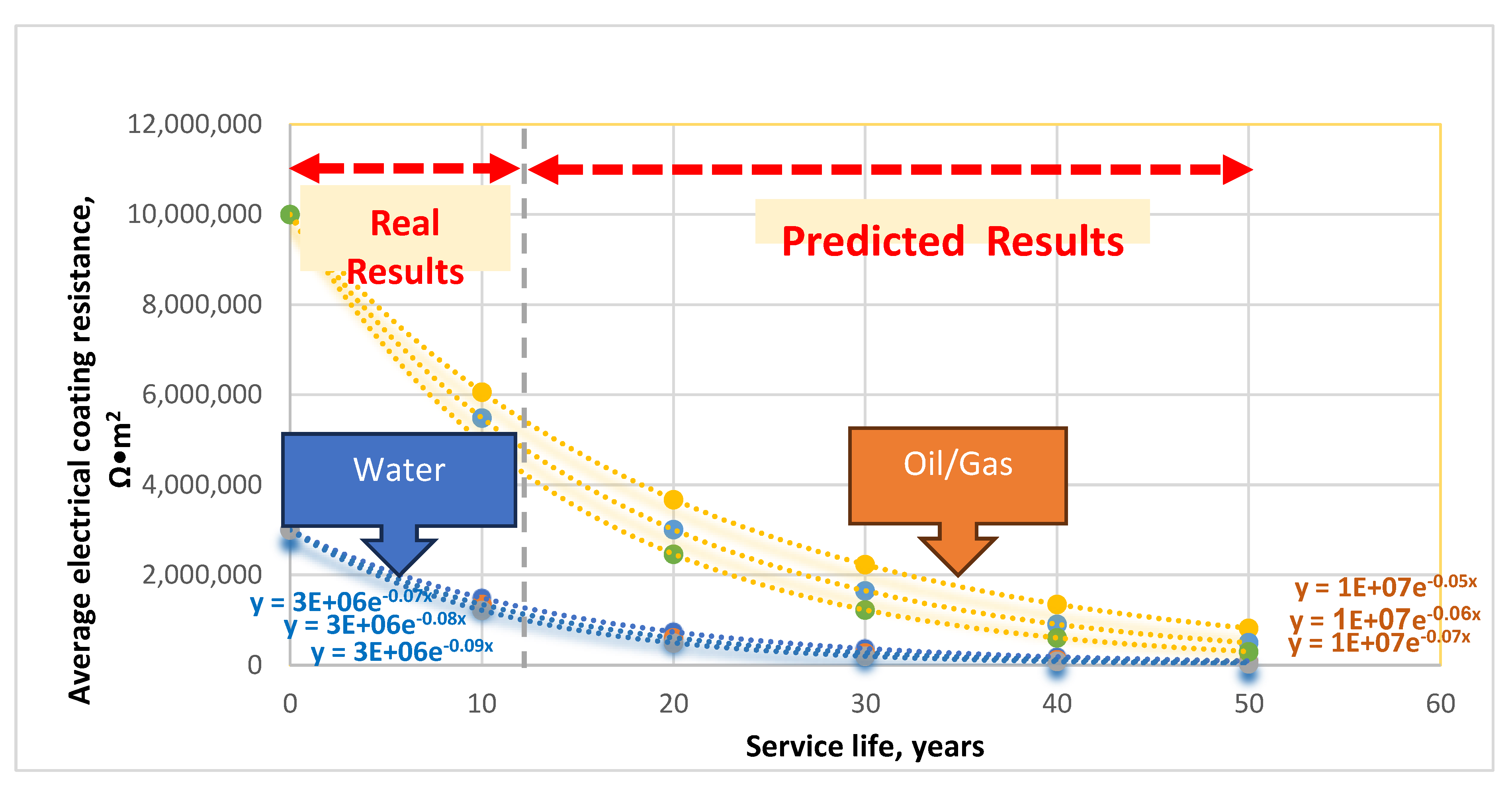

Table 1.
The selected gas/oil pipeline and water pipeline sections for 3LPE coating aging assessment by LCA and DT methods.
Table 1.
The selected gas/oil pipeline and water pipeline sections for 3LPE coating aging assessment by LCA and DT methods.
| Pipeline designation (*) | Diameter (Inch) | Length (m) | Wall thickness (mm) | Pipeline’s age (year) | The initial average specific electrical resistance of the pipeline section, (Ω·m2) (**) |
|---|---|---|---|---|---|
| N1 (N1) South | 16 | 4,920 | 4.0 | 11 | 1,9·106 |
| N2 (N2) South | 20 | 4,990 | 4.0 | 11 | 1.0·106 |
| N3 (N3) South | 24 | 4,940 | 4.8 | 11 | 1.9·106 |
| N4 (N11) Center | 100 | 1,200 | 15.9 | 11 | 4,3·106 |
| G1 (G51) Center | 18 | 9,420 | 12.35 | 11 | 17·106 |
| G2 (G52) Center | 18 | 7,760 | 12.35 | 11 | 11·106 |
| G3 (G53) North | 10 | 14,730 | 10.30 | 11 | 21·106 |
| G4 (G54) North | 18 | 12,540 | 12.35 | 11 | 19·106 |
Table 2.
Summary of coating average specific electrical resistance results of oil/gas and water pipelines using LCA attenuation and DT methods.
Table 2.
Summary of coating average specific electrical resistance results of oil/gas and water pipelines using LCA attenuation and DT methods.
| Pipeline designation (*) | Type of Test | Coating Electrical Resistance, Ω·m2, vs service time, years | ||||
|---|---|---|---|---|---|---|
| Initial (**) | 8 years | 9 years | 10 years | 11 years | ||
| N1 (N1) | Line Current Test | 2.0·106 | - | 1.2·106 | 0.9·106 | 0.7·106 |
| N2 (N2) | Line Current Test | 1.0·106 | - | 0.6·106 | 0.5·106 | 0.4·106 |
| N3 (N3) | Line Current Test | 19.2·106 | - | 8.7·106 | 8.4·106 | 8.7·106 |
| N4 (N11) | Line Current Test | 4.3·106 | - | - | (***) | - |
| G1 (G51) | Line Current Test | 16.9·106 | 10.0·106 | - | 9.6·106 | 9.4·106 |
| Drainage Test | 16.9·106 | - | - | 1.4·106 | - | |
| G2 (G52) | Line Current Test | 10.9·106 | 7.1·106 | - | 6.4·106 | 5.4·106 |
| Drainage Test | 10.9·106 | - | - | 1.4·106 | - | |
| G3 (G53) | Line Current Test | 21.0·106 | - | 11.8·106 | - | 9.1·106 |
| Drainage Test | 21.0·106 | - | - | 0.7·106 | - | |
| G4 (G54) | Line Current Test | 19.5·106 | - | 11.6·106 | - | 9.2·106 |
| Drainage Test | 19.5·106 | - | - | 0.7·106 | - | |
(*) – In brackets, the pipeline numbers from our first study [37]. “N” – for water pipelines; “G” - for oil/gas pipelines. (**) – The initial average specific electrical resistance of the polymer-coated pipeline underground sections after installation and backfilling conducted by the Drainage Test. (***) – The N4 (N11) water pipeline has been crossed with the HVAC power lines (400 kV). The unreliable results obtained with the LCA method make it inappropriate for this technique.
Table 3.
Prediction Model, Coefficients of Determinations, and calculated average aging coefficients of oil/gas pipelines based on LCA method.
Table 3.
Prediction Model, Coefficients of Determinations, and calculated average aging coefficients of oil/gas pipelines based on LCA method.
| Pipeline designation | Prediction model | Calculated average aging coefficient, α, 1/year |
|---|---|---|
| G51 | RC(t)=16.9·106e-0.058t | 0.058 |
| G52 | RC(t)=10.9·106e-0.056t | 0.056 |
| G53 | RC(t)=21.0·106e-0.070t | 0.070 |
| G54 | RC(t)=19.6·106e-0.063t | 0.063 |
Table 4.
Prediction Model, Coefficients of Determinations, and calculated average aging coefficients of water pipelines.
Table 4.
Prediction Model, Coefficients of Determinations, and calculated average aging coefficients of water pipelines.
| Pipeline designation | Prediction model | Calculated average aging coefficient, α, 1/year |
|---|---|---|
| N1 | RC(t)=2.0·106e-0.075t | 0.075 |
| N2 | RC(t)=1.0·106e-0.073t | 0.073 |
| N3 | RC(t)=19.3·106e-0.081t | 0.081 |
Table 5.
Summary of aging coefficients for oil/gas and water pipelines.
| The aging coefficient, 1/year | Oil/Gas Pipelines | Water Pipelines |
|---|---|---|
| Calculated Range | 0.06±0.01 | 0.08±0.01 |
| Average | 0.06 | 0.08 |
| Minimum | 0.05 | 0.07 |
| Maximum | 0.07 | 0.09 |
| The General Prediction Model |
Table 6.
Summarized calculated prediction results of coating average specific electrical resistances (Ω•m2) over time for oil/gas and water pipelines with different aging coefficients (*).
Table 6.
Summarized calculated prediction results of coating average specific electrical resistances (Ω•m2) over time for oil/gas and water pipelines with different aging coefficients (*).
| Service time, years | Oil/gas Pipelines | Water Pipelines | ||||
|---|---|---|---|---|---|---|
| α=0.05 | α=0.06 | α=0.07 | α=0.07 | α=0.08 | α=0.09 | |
| 0 | 1.0·107 | 1.0·107 | 1.0·107 | 3.0·106 | 3.0·106 | 3.0·106 |
| 10 | 6.1·106 | 5.5·106 | 5.0·106 | 1.5·106 | 1.3·106 | 1.2·106 |
| 20 | 3.7·106 | 3.0·106 | 2.5·106 | 0.7·106 | 0.6·106 | 0.5·106 |
| 30 | 2.2·106 | 1.7·106 | 1.2·106 | 0.4·106 | 0.3·106 | 0.2·106 |
| 40 | 1.4·106 | 0.9·106 | 0.6·106 | 0.2·106 | 0.1·106 | 0.8·105 |
| 50 | 0.8·106 | 0.5·106 | 0.3·106 | 0.9·105 | 0.5·105 | 0.3·105 |
(*) – The following assumptions have been made: (a) The prediction exponential aging model: Rc(t)=Rc(0)·exp(-αt) [Ω·m2]. (b) For oil/gas pipelines: the initial coating average specific electrical resistance -1.0·107 Ω·m2. (c) The initial coating average specific electrical resistance for water pipelines is 3.0·106 Ω·m2.
Disclaimer/Publisher’s Note: The statements, opinions and data contained in all publications are solely those of the individual author(s) and contributor(s) and not of MDPI and/or the editor(s). MDPI and/or the editor(s) disclaim responsibility for any injury to people or property resulting from any ideas, methods, instructions or products referred to in the content. |
© 2025 by the authors. Licensee MDPI, Basel, Switzerland. This article is an open access article distributed under the terms and conditions of the Creative Commons Attribution (CC BY) license (http://creativecommons.org/licenses/by/4.0/).
Copyright: This open access article is published under a Creative Commons CC BY 4.0 license, which permit the free download, distribution, and reuse, provided that the author and preprint are cited in any reuse.


