Submitted:
12 November 2025
Posted:
13 November 2025
You are already at the latest version
Abstract
Mobile robot controllers are often complex due to their multi-layered architecture and the numerous inputs and outputs handled at each layer. This work models the lowest level of a differential-drive mobile robot's controller stack using a set of state machines, demonstrating how this approach streamlines control system development. This level handles robot locomotion and sensor data acquisition. The resulting state machines are easily implemented in any procedural language, including C++ and Lua. We use C++ to program controllers for actual Arduino-based robots and Lua to program models of such robots in the CoppeliaSim simulator. Both real and virtual robots have been used in an Embedded Systems course at our university since 2011, with continuous improvements.
Keywords:
mobile robots
; embedded systems
; state machines
; control systems
; robotics education
1. Introduction
The design of controllers for mobile robots presents significant challenges as a result of the numerous tasks they must manage. Although libraries can alleviate implementation details for sensors, actuators, and auxiliary software, describing and implementing robot behavior remains complex.
Typically, behavior is decomposed into different tasks distributed across various tiers of the controller stack or different modules in heterarchical organizations. In layered architectures, for example, a navigation module sits above a path follower, which in turn depends on a locomotion module. Subsumed heterarchy involves modules sharing responsibility for overall behavior at certain levels.
Developing software for such controllers is challenging due to the many components involved and non-functional constraints, including real-time operation and robustness.
Various frameworks (Section 2) exist to model and develop robot controller software. However, these frameworks offer numerous options to accommodate complex controller behaviors. Unfortunately, their advantages in reducing engineering costs come with a steep learning curve, potentially leading to delays and errors from misinterpreted behaviors.
This work aims to minimize non-recurring engineering costs in embedded software development by simplifying the graphical syntax and semantics of state machine diagrams to reduce errors caused by misinterpretation and by streamlining software generation.
A specific goal is to teach students in an Embedded Systems course a methodology to achieve this goal. The main contributions of this methodology are modeling with networks of concurrent state machines and mapping model representations to programming templates.
The course includes a case study in which students develop controller software for mobile robots used in laboratory sessions. Students design and program robots capable of completing missions to reach a destination and return to the starting point. Over time, course materials have been continuously refined, particularly regarding programming templates. The version presented here has been used since 2020, although the original dates to 2011.
This paper presents the structure of the controller stack for a simple differential-drive robot (Section 3). The lower-level controller of this robot (Section 4) executes movement commands and handles lidar-related operations. The latter enables upper levels to scan the area in front of the robot, while the former moves the vehicle to a specified position by changing its pose according to given polar coordinates.
Simplicity arises from the robot’s low-level controller handling movement in two phases: in-place rotation and forward movement (Section 5). This approach simplifies position estimation. Additionally, mathematical computations are simplified because the robot’s kinematic model has its rotation center at the geometric center.
We model this controller’s behavior using state machines that can be easily programmed using templates (Section 6). The process yields embedded software that controls primitive actions of a mobile robot, which can accept commands from upper levels or users.
One advantage of this approach is that even when the target robot’s hardware and components change, the software structure and models remain largely unchanged, with most modifications affecting only small input/output components. Additionally, designers gain better control over execution times and parallelism (concluding section).
2. Literature Overview
Finite-state machine (FSM) models possess formal semantics that simplify behavior specification, verification, and software synthesis. In industrial robotics, particularly, robot operations can be translated into FSMs for repeatable, autonomous execution. For example, Sauer, Hender, and Martens (2019) [1] propose kinesthetic programming where users teach robots procedures by generating state machines that record both operations and sensor data, enabling decision-making when alternative operation sequences exist.
Halim et al. (2022) [2] propose a similar system to teach tasks to robots. However, their operation sequences are limited to guiding robot arm tip trajectories, and state machines represent the main controller’s behavior during learning, teleoperation, or playback modes.
The former system uses an interpreter for generated state machines, while the latter employs hard-coded ones. Both systems demonstrate state machines’ suitability for representing system behaviors without requiring user expertise in state machines or programming.
These cases involve human-machine interfaces using state machines to model high-level robot behavior [1] and user-robot interaction [2], with relatively simple state machine structures. General behaviors require more flexible state machine structures and frameworks supporting development through implementation.
To describe complex behaviors, state machines combine in various ways (parallel or hierarchical organizations) or integrate with other computational models including programs. Explicit hierarchical FSM composition introduces compound states into parent state machines and additional features defining subordinate FSM activation (with history or initial state initiation) and termination (upon reaching end states or exiting their parent compound state).
Numerous frameworks exist for describing state machines. For instance, Samek and Montgomery (2000) [3] presented C/C++ patterns for hierarchical state machines (HSMs) represented by UML state machines, enabling direct mapping between the two. Other similar frameworks include RAFCON [4] and RoboChart [5,6].
RAFCON [4] is a graphical tool for engineering robotic tasks through UML-like HSMs, capable of exporting data for software synthesis tools.
RoboChart [5,6] is a tool based on simplified UML state machines that supports model checking and verification of temporal properties.
Although all these frameworks support code generation, HSMs can also be programmed directly via specialized languages like XRobots [7], where relations between compound states and contained FSMs are established through function-like calls, or using programming patterns [3].
This work employs state-oriented programming based on patterns and templates [8] across different programming languages, without relying on additional libraries. For simplicity, hierarchy is established via handshaking protocols between master and slave modules. This approach greatly simplifies the graphical language semantics and reduces the framework’s learning curve compared to alternatives.
Although state machine diagrams can be programmed manually, automatic translation from diagrams.net (formerly draw.io) drawings to Lua or other programming languages can be achieved using our custom tool [9] or, more recently, using artificial intelligence (AI) tools. While no direct link to model checking tools exists, properties can be tested dynamically by including specific methods in corresponding state machine classes, and specific loggers can capture execution traces.
Robot controller behaviors are typically described using multiple state machines organized as HSMs [10] or layered architectures, as in our proposal where no explicit hierarchical dependencies exist. Combinations are also possible. For example, YASMIN [11] enables designing state machines that communicate through a blackboard and synthesizing code for some modules of a predefined architecture on top of ROS2. Here, descriptions are not limited to HSMs but can include behavior trees (BTs).
Other options for higher-level behavior descriptions include dynamic stack deciders [12], a type of stack automata capable of changing action plans by modifying the state stack with decision trees. Simulating stack automata is possible in our case because we use extended FSMs (EFSMs) with extended memory that can be changed from cycle to cycle in the same way as the main state.
This work focuses on the lower levels of the robot controller stack, where actuation plans remain constant. In this regard, it closely relates to earlier work from 2004 [13], where algorithmic state machines (ASMs) and FSMs modeled drivers and the L0 level of a mobile robot. However, that work constrained models to binary inputs and outputs (each corresponding to a micro-operation), like the control part of an external operational unit. Our EFSMs are unconstrained, allowing changes to both the main state and additional state variables during transitions.
Although transitions in state machines modeling high-level robot operations and decision-making processes are not highly constrained, some steps may require continuous control output updates or guarantees of timely discrete-time updates. This is particularly relevant for robot movement, where locomotion controllers are modeled as discrete-time state machines that can operate in continuous mode at certain states, i.e., as hybrid state machines.
For differential-drive robots, simple modifications to control variables applied at high rates can approximate continuous operation. For example, Rustam et al. [14] presented a simple control algorithm for straight-line movement that applies small step changes to control variables based on sideways drift. In our case, steps derive from an analytical model and are proportional to the error and a derivative factor to prevent single-cycle error correction.
Indeed, controllers based on proportional-integral-derivative (PID) formulations are commonly used, with parameters identified to achieve smooth robot operation [15,16].
Some works enable robots to reach specific target points given in polar coordinates without prescribed trajectories, while others constrain robot movement to specific paths like curved trajectories [17]. The latter cases require more complex expressions than simple PID formulations [18] to adjust control variables for accurate, smooth movement along predefined trajectories.
In other cases, reference trajectories are generated dynamically. For instance, [19] presented a wheelchair control combining user control variables with controller variables following curvilinear trajectories. This offers another perspective on adjusting control variables considering the robot’s actual trajectory and variable references, such as when obstacles appear suddenly.
In our case, state machines controlling robot wheels include states with quasi-continuous PID control modes that divide trajectories into two parts: orientation change and straight movement to the destination.
3. Controller Stack
The robots must navigate their environment to complete a given mission. A typical mission involves reaching a specific point to, for example, pick up or deliver materials.
Programming the corresponding controller requires first designing its behavioral model, preferably independent of implementation details. This work uses a network of interacting state machines, each modeling a controller component’s behavior.
Before detailing state machines, we must define the controller architecture, describing system components and their communication. We represent components with large rectangles, signals with squares, and communications’ directions with arrows.
Signals are updated “continuously,” meaning that in this discrete system, they are computed at every state machine transition. They may possess memory, so they need not be computed at each cycle, or conversely, they may be updated spuriously. We use circles inscribed in squares to represent signals with memory, and circles alone for variables, i.e. data containers with memory not necessarily attached to communication signals.
All module inputs are memoryless signals, while outputs can be memoryless or attached to variables. Since pure output signals may create undesired combinatorial feedback loops causing signal value determination issues, all output signals derive from variables.
A combinatorial feedback loop occurs when an input signal’s value at a given time depends on a pure output signal from the same module at the same time, directly or indirectly. This situation makes signal values difficult to predict, as they depend on system implementation specifics.
We use a layered architecture (Figure 1) for the robot controller to progressively decompose general missions into detailed actions.
The simplest mobile robot mission involves moving from its current position to a target location by following given path steps. More complex missions provide only the destination, with or without complete environment maps, requiring exploration and mapping.
The controller stack’s highest level (L2) takes a path P and guides the vehicle along it until either complete traversal or failure, returning to the initial point. (While more complex behaviors can be added, they fall outside this paper’s scope.)
L2 commands split into an operation code W and an optional path T. Input W can be ’F’ (follow path), ’S’ (lidar sweep), or ’Q’ (quit current operation and wait). For the mission at hand, L1 takes path T and sends actions to the lower level. These actions consist of commands executed by the L0 layer.
L0 layer commands are triplets containing the operation code (0: none, 1: GO, 2: LIDAR, 3: RESUME, 4: HALT), angle , and distance r. The last two are used only for GO instructions.
L0 transforms each GO command into corresponding left (L) and right (R) motor control values until the vehicle reaches the destination. These values, along with whether the robot has reached its final pose, depend on wheel encoder data and . Upon completing an action or encountering unexpected events, L0 sends an appropriate message M to the upper level.
Additionally, L0 communicates with the lidar module to direct it to a specific angular position W and retrieve the distance to objects E (from echo). Beyond obstacle detection during forward movement, this communication enables scanning distances to objects across the 180-degree front field of view.
The controller’s lowest level contains device drivers, which take DC motor control values for left and right wheels and the servomotor adjusting lidar orientation, providing L0 with encoder and lidar data.
All components integrate into a framework including an Arduino-compatible board and Bluetooth communication module (Figure 2). Front and rear caster wheels provide stability during movement. The kinematic center is located at the robot’s geometric center to simplify position computations. Similarly, the lidar is positioned above the platform center.
4. L0 Model
This layer executes four basic actions: GO, LIDAR, RESUME, and HALT. Action GO moves the vehicle to a specified position in polar coordinates relative to its kinematic center, while LIDAR sweeps a 180 front field of view. For simplicity, GO and LIDAR commands cannot be executed in parallel. However, the lidar is used to detect obstacles directly ahead during movement. The LIDAR command initiates a lidar sweep but requires L1 to RESUME after each reading.
HALT stops any ongoing command execution and, during lidar sweeps, returns the lidar sensor to forward orientation. Accurate lidar readings require the servomotor to be stationary, but the L0 controller can communicate with higher levels regardless of whether it is rotating or not. Although this parallel behavior is less critical during forward movement, it becomes useful during lidar sweeps, where sending data to L1 and rotating the servomotor to target orientation can occur simultaneously. Thus, L0 divides into two controllers: L0Main and L0Lidar. The former handles communication with L1 and locomotion, while the latter manages lidar orientation and readings (Figure 3).
Communication between L0Main and L0Lidar is relatively simple: L0Lidar sets u (update) to true when a new distance Q to an object is computed. L0Main directs L0Lidar to point to specific angles by setting A accordingly.
The L0Lidar state machine (Figure 4) starts by setting the lidar orientation to 0. After initialization, it performs continuous measurements, acquiring new values as rapidly as possible.
In Figure 4, nodes represent state machine states, and arrows are labeled with conditions triggering transitions to next states. These labels may include immediate actions (e.g., function calls) or delayed actions. Delayed actions take effect when the state machine completes a transition, even if it remains in the same state.
We use extended finite state machines (EFSM). Graphs show main state values and possible state transitions. In these machines, the state extends with variables, which are data containers beyond the main state. Next variable values are denoted by a superscript plus sign (plain text appends a plus), and assignments to next values are delayed, meaning variables change when the main state changes.
In Figure 4, the arrow pointing to the initial state ROTATE has a constant true condition, always firing at start, with actions setting initial variable values: begin time B to current real time T; servomotor delay to point to 0D to , where _wrot is motor angular speed in degrees per second; target angle Y (yaw) to 0; control value Z to the value for 0 degrees from function y2z(); pending request p to false; obstacle distance Q to 0 (default for undetected objects); and update flag u to false.
Each state associates with a specific output signal s value, true for only one cycle to signal the lidar driver to wait for a new reading. The state machine can interact with external modules with or without explicit communication of detected distances. The former case involves input signal r (request) and variables p (pending request) and u (update acknowledgement), described next.
In the ROTATE state, the machine waits for the servomotor to turn degrees (or 90 degrees initially). It waits D seconds, computed using the servomotor’s average rotation speed _wrot, and sets servomotor control output Z. The value assigned to Z comes from function y2z(), which translates angles to appropriate control values. Argument 360 returns 360, indicating no control signal sent to the servomotor.
At PING, it checks if the input orientation angle A matches the lidar’s current position Y. If they match, it moves to ECHO to wait for distance reading E and sets output s (send ping) to true. If Y differs from A, the state machine returns to ROTATE to orient the lidar to angle A, and Y is set to A.
When using the handshake protocol, the client module sets r to true and A to the desired angle, then waits for u to become true. The L0Lidar state machine stores r into p if the request occurs during rotation (ROTATE) or when requesting a new lidar reading (PING), and sets u to true only if p is true, i.e., only the first reading after u becomes true.
The L0Main behavior involves listening for L1 commands and replying with execution results. Thus, the initial and idle state is LISTEN (Figure 5), waiting for incoming commands. From this state, it can transition to states corresponding to GO and LIDAR commands. RESUME and HALT have no effect here except sending error messages.
When (lidar sweep), L0Main transitions from LISTEN to LIDAR (Figure 6), checking if the next scan angle in table _scan is not 360, which marks the sweep end. If not, it moves to ECHO, waiting for an update on input value Q via u.
Upon receiving a positive pulse (true) on u, the state machine transitions to RAY to send data to the upper level via output M. From RAY, it proceeds to RESUME to await a RESUME command from the upper level. From RESUME, it transitions to ECHO or DONE, depending on whether the next angle differs from 360.
Since the angle list in _scan may not end with 0, if _scan[J] is 360, L0Main instructs L0Lidar to point forward by setting P to 0 and transitioning to DONE, waiting for the next lidar update confirming forward orientation. Note that in transitions from ECHO, RAY, and RESUME to DONE ensures the lidar returns to its initial setting.
The other L1 command is GO, causing L0Main to switch to TURN or GO states (Figure 7). For GO with non-zero angle, it first goes to TURN, then to GO if distance is positive. For GO with only non-zero distance, it moves directly to GO. Transitions to TURN and GO also set variables L and R to and values for left/right turns or forward movement.
Initially, and are set to and and remain unchanged in this on-off controller mode. However, Section 5 presents a better control strategy where these values adjust to refine robot movement and minimize final pose errors.
In the TURN state, it updates angle A, distance S, and X and Y position errors relative to the goal at polar coordinates . Function computes the next distance error to the goal. Inputs and contain angle and linear displacement variations since the last cycle, computed from left and right encoder count increments and . Because updates occur next cycle, all arc conditions use current A, S, X, and Y values.
The state machine leaves TURN when the next angle magnitude falls below angle tolerance _atol: it returns to LISTEN if the goal is within distance tolerance _stol, or moves to GO to start forward movement otherwise. In the first case, L and R are set to 0 to stop the vehicle; in the second, they are set to uL and uR for forward motion.
In GO, variables A, S, X, and Y are updated, and next values determine if the final position is reached within tolerance _stol on X (negative). To prevent collisions, the distance to front obstacles Q must exceed safe distance _sdist. If , the state machine transitions from GO to BLOCKED, checking if the front obstacle moves away within _tout seconds. If Q exceeds _sdist before timeout, it returns to GO; otherwise, it moves to LISTEN.
From TURN, GO, and BLOCKED, the state machine returns to LISTEN when (HALT), setting L and R to 0 and M to an appropriate text message. Commands other than HALT receive warning messages indicating command ignorance.
To simplify the above explanation, L and R are constant in both TURN and GO states. In practice, they would have to be modified every cycle to account for motion errors, especially when moving forward. Thus, L and R would have to be updated every cycle with the same values of uL and uR, which would be calculated to compensate for any motion errors. Obviously, in transitions to BLOCKED or LISTEN, L and R would become 0. The next section will show how to update uL and uR in discrete control modes that simulate continuous control.
5. Movement Control
Commands transform into an -degree rotation (positive to the right) followed by an r-cm forward movement. This simplifies robot position tracking and control. Variables A and S store angle and distance errors in radians and mm, respectively. Initially zero, they add and r upon receiving a GO command.
The control strategy drives A and S to 0 within tolerance by adjusting output variables and , containing DC control values for left and right motors. This section enhances the previously described on-off control system to discrete control by updating and each cycle.
To determine their values based on pose error each iteration, left and right wheel movements in mm, and , are computed as:
where are positive or negative encoder count increments since last reads, is wheel radius, and CPR is counts per revolution (1440 in our case).
These values transform into and , containing average angle variation in radians and average forward movement in mm:
where is the distance between wheels.
The movement’s first phase (rotation) progressively adds dA to A until A reaches 0 within tolerance:
The second phase moves the vehicle forward, progressively decreasing S by dS if no heading error exists, updating robot position accordingly. However, since A may not be zero at this phase’s start and slight speed differences may cause drift, an error correction mechanism is necessary. The error is the yaw angle A relative to the target vector.
At each cycle, the current position , the yaw angle (), and the target distance are calculated from the last position of the vehicle with respect to the target , the last yaw angle A, and and :
Using these values, left and right motor control values and are computed to approach the target and correct heading angle. The target distance is known (), but the rotation angle () compensating for yaw to point to the target must be computed (see Figure 8):
Knowing that the motor speeds are proportional to and , and that they have caused a change in pose of in polar coordinates, the new values would cause a linear movement and a change in orientation that would compensate for the heading error :
where and are limited to range , the minimum for DC motors to move the robot and the maximum to limit vehicle speed.
This control strategy is highly sensitive to controller cycle time because for relatively short timesteps, magnitudes can resemble magnitudes. Small angle error variations could cause large control value changes, potentially leading to aggressive corrections by attempting full compensation in one cycle.
A better proportional controller would compensate for an eA fraction each control cycle. Note that when , the robot should turn right, so the right motor should reduce speed proportionally while the left maintains maximum speed (), and vice versa for .
The formulas for and imply subtracting a value from on the turn side:
The subtracted value is a fraction of the control span () proportional to the relative yaw error eA. Note that is 0 when and when , and is when and 0 when .
We assume a maximum yaw error eA of (), providing a good compromise between smooth movement and precision based on experimental data. For high-precision robots, this value can be smaller, enabling more aggressive braking and quicker orientation error correction.
In practice, however, we use a PID controller adding a derivative factor to distribute error correction over more cycles. The expressions resemble Equations 10 and 11:
where is the error variation since the previous cycle and is the cycle time. Constants and are determined experimentally, with the initial Kp guess being K from Equation 12. Although not perfect, this PID controller operates more smoothly than previous versions.
To minimize sudden stops, should reduce as the robot approaches the goal or obstacles. Here, decreases proportionally to the distance to nearby obstacles between (braking distance) and _sdist (safety distance) down to . Values below cannot move the vehicle, so the transition from to 0 is seamless.
6. Programming
Implementing the controller stack involves synthesizing software from its computational model. In this case, a network of concurrent EFSMs organized into three layers is transformed into Lua and Arduino Sketch programs. The full controller stack is implemented in the CoppeliaSim simulator, and L0 is implemented in Arduino Sketch for the robot’s Arduino-compatible processor.
The embedded L0 controller (shaded part in Figure 9) communicates with upper levels via a Bluetooth serial profile link. An additional layer, L0L1Link, makes L1 communication transparent regardless of whether one robot (virtual or real) or both are used. L1 messages are sent to both, and L0 messages are synchronized with priority given to real-world messages. (More sophisticated strategies are possible but beyond this work’s scope.)
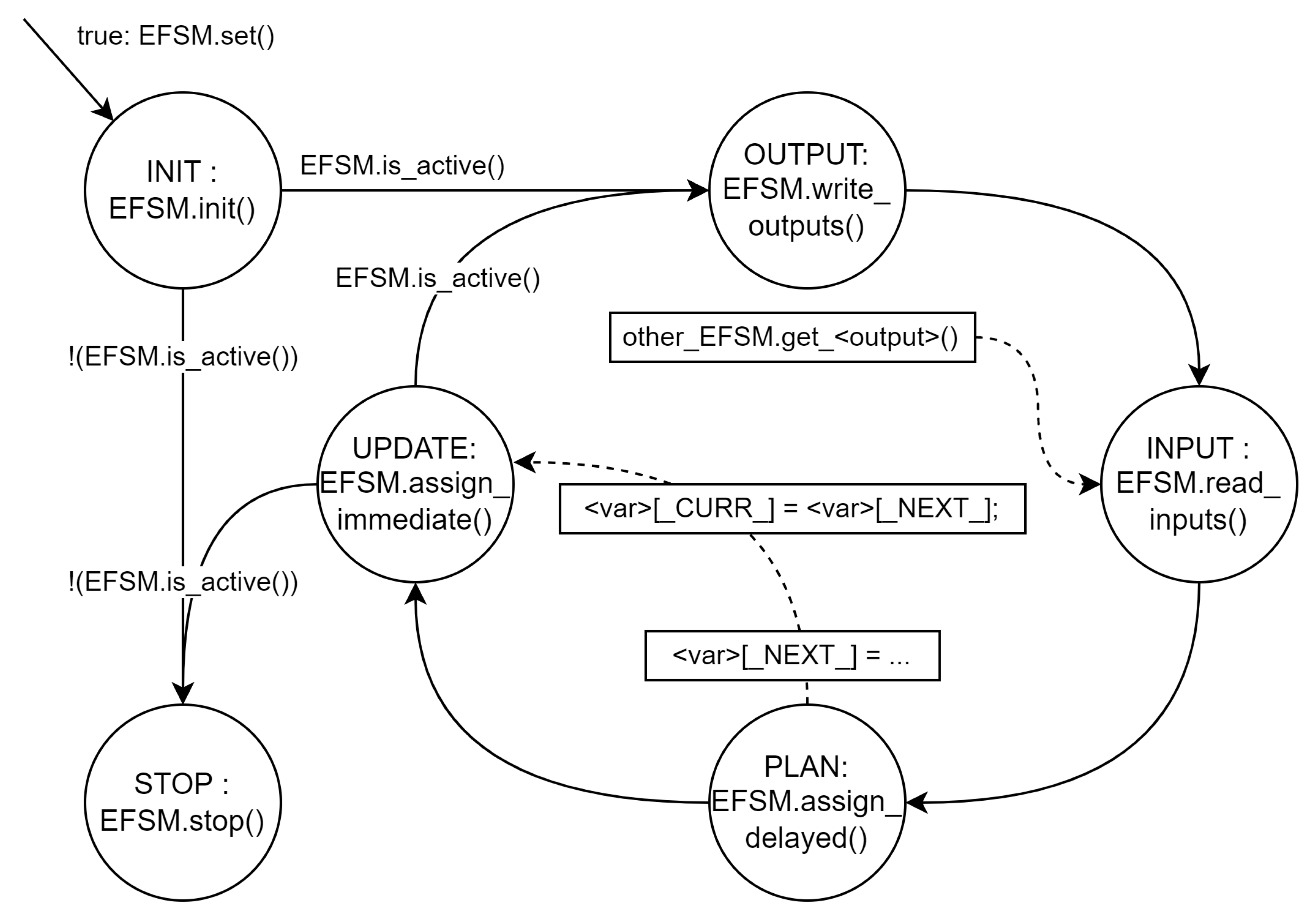
To synthesize the software corresponding to the L0 level, two independent modules are generated: L0Main and L0Lidar. Each one contains the definition of the corresponding class, with methods to execute each of the operations it must perform to evolve in time and which are illustrated in Figure 10: After preparing the object according to the configuration parameters that have been given to it with set and initializing the extended state and the immediate outputs with init, it passes to a loop that only stops in case the is_active method returns false.
The is_active method indicates whether the EFSM is in an active state or has reached a sink state, that is, without output arcs, whether this is expected or due to an error. In this case, EFSMs have no final state and can therefore only exit the loop if there is an error. In practice, however, in the event of an error, the state machine is reset and the loop continues.
The loop begins with a call to write_outputs to transfer the contents of the output signals to the devices they have connected, be it a program window in the case of an interactive simulation or microcontroller ports in the case of the real robot. It continues by calling read_inputs to obtain the data for the input signals, to be able to determine the values of the extended state (main state and complementary variables) for the next state (assign_delayed) and, finally, to make the next state the current one, completing the assignment of the values of the next extended state to the current extended state and determining the values of the immediate outputs (assign_immediate).
Listing 1 shows an Arduino Sketch fragment simulating L0 state machines following this procedure. After instantiating both objects, the setup function calls their set and init methods to create necessary data structures and objects and initialize them appropriately.
| Listing 1. Simulation engine in Arduino Sketch |
| 1 #include "L0Lidar.h" |
| 2 #include "L0Main.h" |
| 3 L0Lidar Lidar(LIDAR_SERVO); |
| 4 L0Main Main(M1DIR, M1PWM, /* ... */); |
| 5 void setup() { |
| 6 Lidar.set(); Main.set(); |
| 7 Lidar.init(); Main.init(); |
| 8 } // setup |
| 9 unsigned long dt = 25; // [ms] |
| 10 void loop() { |
| 11 unsigned long starttime = millis(); |
| 12 Lidar.write_outputs(); Main.write_outputs(); |
| 13 Lidar.read_inputs(Main.get_target()); |
| 14 Main.read_inputs(Lidar.get_distance(), Lidar.get_update()); |
| 15 Lidar.assign_delayed(); Main.assign_delayed(); |
| 16 Lidar.assign_immediate(); Main.assign_immediate(); |
| 17 if(!Lidar.is_active()) {Lidar.init();} |
| 18 if(!Main.is_active()) {Main.init();} |
| 19 while (millis()-starttime<dt) {;} |
| 20 } // loop |
The loop function implements the DO-OUTPUT-INPUT-PLAN cycle from Figure 10 for each EFSM. Unlike the figure’s behavior, if any state machine becomes inactive, it resets internal data by calling its init method and resumes the loop. More sophisticated actions like activating error handling could be taken when state machines become inactive due to failures.
The final while ensures no cycle runs shorter than dt milliseconds, preventing oversampling issues like excessive power consumption from input/output operations.
The objects link via read_inputs calls with arguments from the other object obtained through get_signal methods. Here, L0Lidar has one input from L0Main specifying the lidar target angle, and L0Main has two inputs from L0Lidar: obstacle distance (Q) and update status (u).
Each object class must contain methods called in the simulation engine (lines 04 to 12 in Listing 2) and private variables for EFSM input signals, state, model variables, and outputs (lines 17 to 28 in Listing 2).
| Listing 2. EFSM header file for L0Lidar |
| 1 class L0Lidar { |
| 2 public: |
| 3 L0Lidar( ... ) |
| 4 void set() { ... } |
| 5 void init(); |
| 6 void write_outputs(); |
| 7 long get_distance(); |
| 8 bool get_update(); |
| 9 void read_inputs(float angle); |
| 10 void assign_delayed(); |
| 11 void assign_immediate(); |
| 12 bool is_active(); |
| 13 private: |
| 14 char _SERVOPIN; |
| 15 Servo _Servo; |
| 16 VL53L0X _Sensor; |
| 17 float _wrot; // Rot. speed [deg/s] |
| 18 int A; // Target angle [deg] |
| 19 unsigned E; // Obstacle dist. [mm] |
| 20 enum {S_ROTATE, S_PING, S_ECHO, |
| 21 S_SINK} state[2]; |
| 22 int Y[2]; // Yaw |
| 23 float Z[2]; // Servo position |
| 24 float B[2]; // Begin time |
| 25 float D[2]; // Delay |
| 26 float Q[2]; // Distance to obstacle |
| 27 bool u[2]; // Distance update |
| 28 bool s[2]; // Send ping |
| 29 int Y2Z(int A); |
| 30 }; |
All variables representing the extended state (the state itself and other model variables) are two-element arrays, the first holding the current iteration value (_CURR_) and the second the next cycle value (_NEXT_). Thus, delayed assignments first set the _NEXT_ item value, and the immediate assignment phase copies this value to the _CURR_ field. (Immediate outputs are set according to current model variable values, including the state variable.)
Distinguishing _CURR_ and _NEXT_ values prevents errors from incorrect instruction execution order in assign_delayed. For example, swapping lines 9 and 10 in Listing 3 would make variable D always zero because Y would be set to A before computing D’s new value.
This guarantee requires a second method to update all EFSM variables and output signals: assign_immediate, partially shown in Listing 3.
| Listing 3. Delayed and immediate assignments in L0Lidar |
| 1 void L0Lidar::assign_delayed() { |
| 2 if (state[_CURR_]==S_ROTATE) { |
| 3 if (T-B[_CURR_]>=D[_CURR_]) { |
| 4 Z[_NEXT_] = Y2Z(360); state[_NEXT_] = S_PING; |
| 5 } // if |
| 6 } else if (state[_CURR_]==S_PING) { |
| 7 u[_NEXT_] = false; |
| 8 if (A!=Y[_CURR_]) { |
| 9 B[_NEXT_] = T; D[_NEXT_] = abs(A-Y[_CURR_])/_wrot; |
| 10 Y[_NEXT_] = A; Z[_NEXT_] = Y2Z(A); |
| 11 state[_NEXT_] = S_ROTATE; |
| 12 } else { // A==Y[_CURR_] |
| 13 s[_NEXT_] = true; state[_NEXT_] = S_ECHO; |
| 14 } // if |
| 15 } else if (state[_CURR_]==S_ECHO) { |
| 16 s[_NEXT_] = false; |
| 17 if (E>=0 ) { |
| 18 u[_NEXT_] = true; Q[_NEXT_] = E; state[_NEXT_] = S_PING; |
| 19 } // if |
| 20 } else { // error handling |
| 21 } // if chain |
| 22 } // L0Lidar::assign_delayed() |
| 23 void L0Lidar::assign_immediate() { |
| 24 state[_CURR_] = state[_NEXT_]; |
| 25 Y[_CURR_] = Y[_NEXT_]; Z[_CURR_] = Z[_NEXT_]; |
| 26 // (... omitted ...) |
| 27 } // L0Lidar::assign_immediate() |
read_inputs and write_outputs methods are platform-specific and must be programmed to read data into state machine inputs or take outputs from them and perform actions like sending serial port messages. Outputs intended for other state machines require get_signal methods, called to supply arguments to other state machines’ read_inputs. This code organization enables direct binding between graph elements and program instructions, making programming systematic and easily automatable.
7. Discussion
This work developed a complete state-based model for the reactive-level controllers of a differential-drive robot. The concurrent EFSMs model can simulate hierarchy while maintaining simple transition semantics, reducing the learning curve. Indeed, the original motivation for prioritizing simple semantics was classroom adoption.
Our experience shows that while students struggle with extended state concepts and timely signal updates, they achieve good understanding of parallel system operation, module communication, data sharing, priority setting, and the development process. Satisfaction surveys show positive ratings for embedded systems courses with this content, particularly the opportunity to work with real robots in the laboratory.
The model also integrates hybrid state machine concepts where some states have discrete control modes.
The programming templates and patterns presented have evolved from expert-programmer-style code to simpler schemas focusing on code-graph correlation.
We also highlighted the embedded software development process from state machine network models.
Although the generated embedded software is functionally correct and works well in some environments, non-functional requirements like controller duty cycles may not be met on certain platforms. Unoptimized code contained approximately 700 lines of code (LoC), occupying 60 Kb of code memory and 8 Kb of data memory on an Arduino Teensy board, with an average cycle time of 31 ms. For proper PID controller operation, shorter cycle times were needed, prompting code optimization. The result is a 600 LoC program without arrays and global variables, using 58K of code memory and 7 Kb of data memory with an average cycle time of 12 ms.
In summary, we presented a state-based modeling and embedded software development process for robot controllers capable of modeling HSM, BT, and hybrid systems while maintaining simplicity and high model-code correlation. Implementation requires adapting I/O for each case—interactive simulation, virtual environment robot simulation, or real robots. The final development stage involves program optimization to meet system non-functional requirements.
Although graphical representation translation into programs can be manual using provided templates and examples, or automatic with specialized tools, we are exploring how AI can follow programming patterns with appropriate prompting to generate reliable code. We believe AI tools can support robot controller design and development engineering and that training future engineers in this area is necessary.
Funding
This research received no external funding.
Data Availability Statement
Diagrams and software are available upon request.
Acknowledgments
The author thanks Jordi Guerrero for building the robot and conducting tests, and Ismael Chaile, Pragna Das, Joaquín Saiz, and Daniel Rivas for their contributions to various versions of the physical and virtual robots over the years.
Conflicts of Interest
The author declares no conflicts of interest.
Abbreviations
The following abbreviations are used in this manuscript:
| ASM | Algorithmic State Machine |
| BT | Behavior Tree |
| EFSM | Extended Finite State Machine |
| FSM | Finite State Machine |
| HSM | Hierarchical State Machine |
| LoC | Lines-of-Code |
| PID | Proportional-Integral-Derivative |
| UML | Unified Modeling Language |
References
- Sauer, L.; Henrich, D.; Martens, W. Towards Intuitive Robot Programming Using Finite State Automata. In KI 2019: Advances in Artificial Intelligence: 42nd German Conference on AI, Kassel, Germany, September 23–-26, 2019, Proceedings. Springer-Verlag, Berlin, Heidelberg, 290–298. [CrossRef]
- Halim, J.; Eichler, P.; Krusche, S.; Bdiwi, M.; Ihlenfeldt, S. No-code robotic programming for agile production: A new markerless-approach for multimodal natural interaction in a human-robot collaboration context. Frontiers in Robotics and AI, 9, 2022. [CrossRef]
- Samek, M.; Montgomery, P. State-oriented programming. Embedded Systems Programming 13(8), 2000, 22–43.
- Brunner, S.G.; Steinmetz, F.; Belder, R.; Dömel, A. RAFCON: A Graphical Tool for Engineering Complex, Robotic Tasks. In: IEEE/RSJ International Conference on Intelligent Robots and Systems (IROS), 3283—3290, 2016, Daejeon, South Korea. [CrossRef]
- Li, W.; Miyazawa, A.; Ribeiro, P.; Cavalcanti, A.; Woodcock, J.; Timmis, J. From Formalised State Machines to Implementations of Robotic Controllers. In: , et al. Distributed Autonomous Robotic Systems. Springer Proceedings in Advanced Robotics, vol 6. Springer, Cham. 2018. [CrossRef]
- Miyazawa, A.; Ribeiro, P.; Li, W.; Cavalcanti, A.; Timmis, J.; Woodcock, J. RoboChart: modelling and verification of the functional behaviour of robotic applications. Software & Systems Modeling. 18, 1–53. 2019. [CrossRef]
- Tousignant, S.; Van Wyk, E.; Gini, M. An Overview of XRobots: A Hierarchical State Machine Based Language. In: ICRA-2011 Workshop on Software Development and Integration in Robotics, Shanghai, China May 2011.9–13.
- Ribas-Xirgo, Ll. How to code finite state machines (FSMs) in C. A systematic approach. 2014. [CrossRef]
- Rivas, D.; Das, P.; Saiz-Alcaine, J.; Ribas-Xirgo, Ll. Synthesis of Controllers from Finite State Stack Machine Diagrams. IEEE 23rd International Conference on Emerging Technologies and Factory Automation (ETFA), 2018, 1179–1182. [CrossRef]
- Zhou, H.; Min, H.; Lin, Y.; Zhang, S. A Robot Architecture of Hierarchical Finite State Machine for Autonomous Mobile Manipulator. In: Huang, Y., Wu, H., Liu, H., Yin, Z. (eds) Intelligent Robotics and Applications. ICIRA 2017. Lecture Notes in Computer Science, 10464. Springer, Cham.. 425–436. [CrossRef]
- González-Santamarta, M.Á.; Rodríguez-Lera, F.; Fernández, C.; Martín, F.; Matellán, V. YASMIN: Yet Another State MachINe library for ROS 2. 2022. [CrossRef]
- Poppinga, M. & Bestmann M. DSD – Dynamic Stack Decider. International Journal of Social Robotics. 14:73–83. Springer. (2022). [CrossRef]
- Levin, I.; Kolberg, E.; Reich, Y. Robot Control Teaching with a State Machine-based Design Method. International Journal of Engineering Education, 20(2), 2004.
- Rustam, I.; Tahir, N.M.; Yassin, A.I.M.; Wahid, N.; Kassim. A.H. Linear Differential Driven Wheel Mobile Robot Based on MPU9250 and Optical Encoder. TEM Journal 11(1), 30—36, February 2022. [CrossRef]
- Myint, C.; Win, N.N. Position and Velocity control for Two-Wheel Differential Drive Mobile Robot International Journal of Science, Engineering and Technology Research (IJSETR) 5(9), September 2016.
- Hirpo, B.D.; Zhongmin W. Design and Control for Differential Drive Mobile Robot. International Journal of Engineering Research & Technology (IJERT), 6(10), 2017. 327–334.
- Dòria-Cerezo, A.; Biel, D.; Olm. J.M.; Repecho, V. Sliding mode control of a differential-drive mobile robot following a path. 18th European Control Conference (ECC), 2019, 4061—4066. [CrossRef]
- Nurmaini, S.; Dewi, K.; Tutuko, B. Differential-Drive Mobile Robot Control Design based-on Linear Feedback Control Law. IOP Conference Series: Materials Science and Engineering, Volume 190, IAES International Conference on Electrical Engineering, Computer Science and Informatics 23–25 November 2016, Semarang, Indonesia. [CrossRef]
- Tafrishi, S.A.; Ravankar, A.A.; Salazar Luces, J.V.; Hirata, Y. A Novel Assistive Controller Based on Differential Geometry for Users of the Differential-Drive Wheeled Mobile Robots, arXiv:2202.01969v1, 4 Feb. 2022. [CrossRef]
Figure 1.
Controller structure.
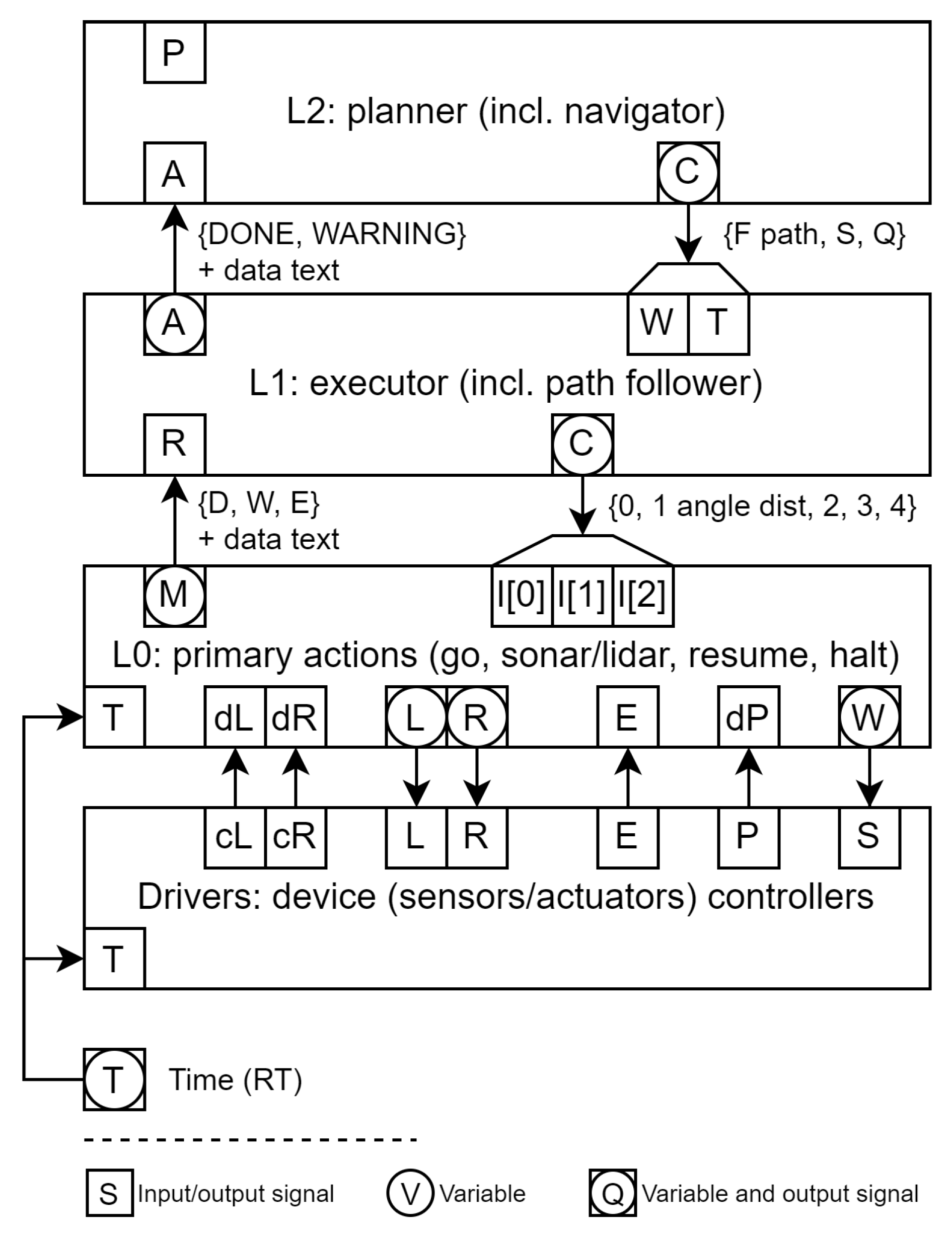
Figure 2.
The mobile robot incorporates essential hardware for communication, world sensing, and closed-loop control movement.
Figure 2.
The mobile robot incorporates essential hardware for communication, world sensing, and closed-loop control movement.
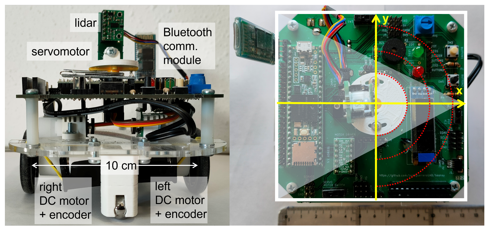
Figure 3.
Layer L0 divides into L0Main and L0Lidar modules for concurrent operation.
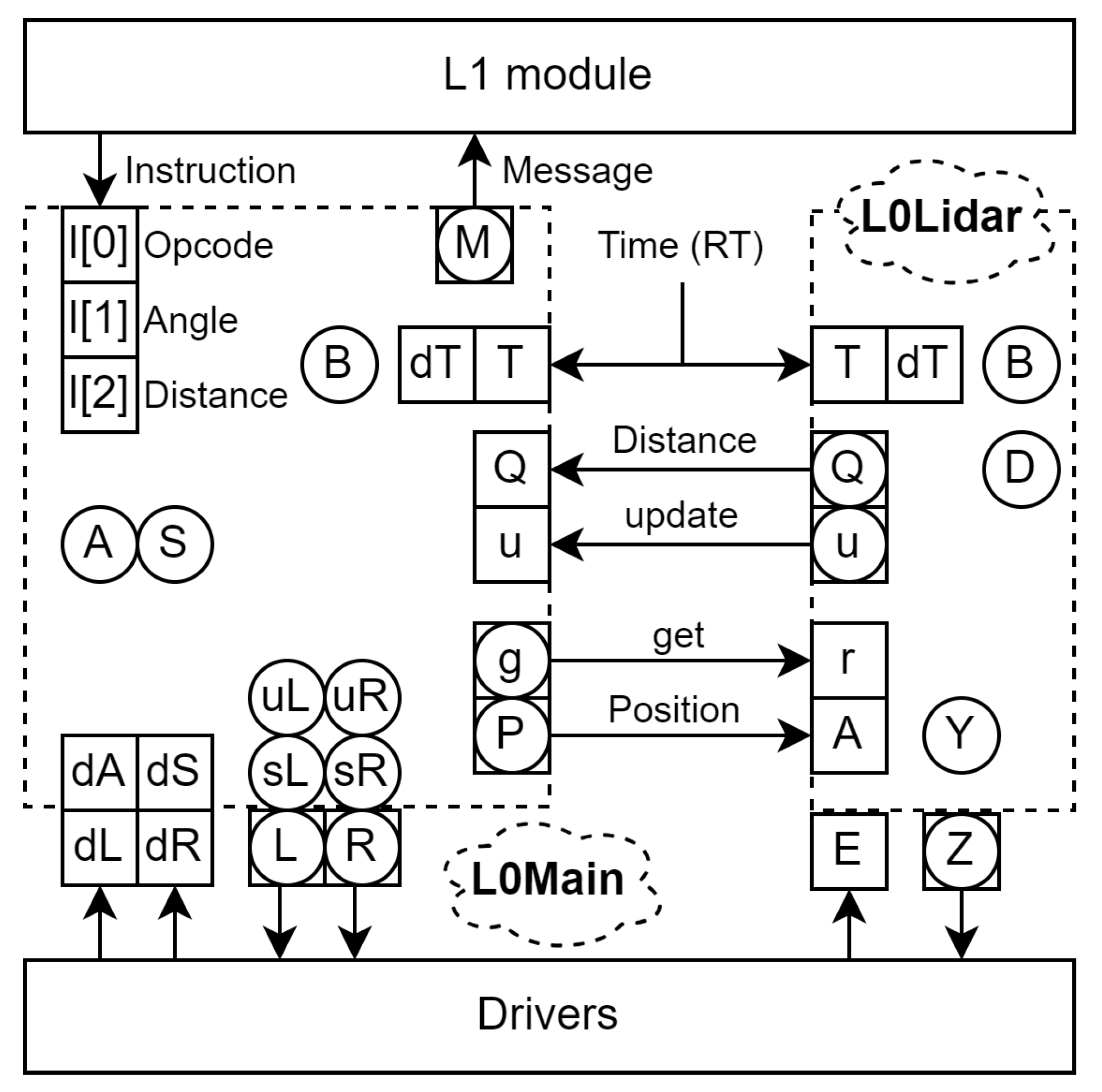
Figure 4.
EFSM model of the lidar controller behavior.
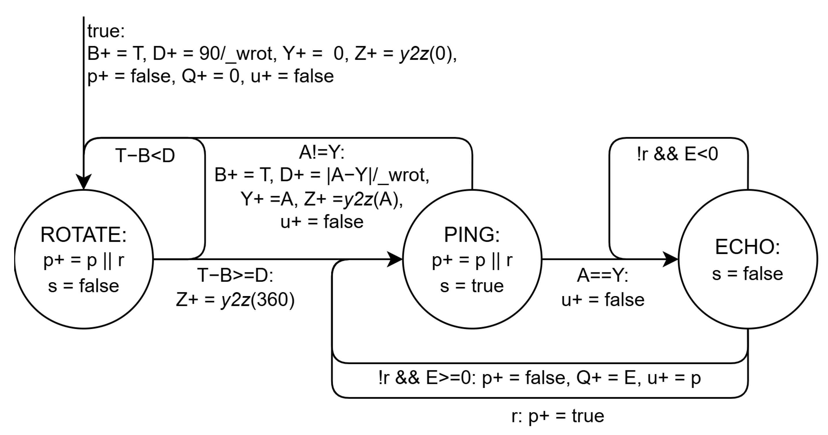
Figure 5.
The L0Main controller’s initial and idle state is LISTEN. Upon receiving a valid command, it transitions to either LIDAR or GO.
Figure 5.
The L0Main controller’s initial and idle state is LISTEN. Upon receiving a valid command, it transitions to either LIDAR or GO.
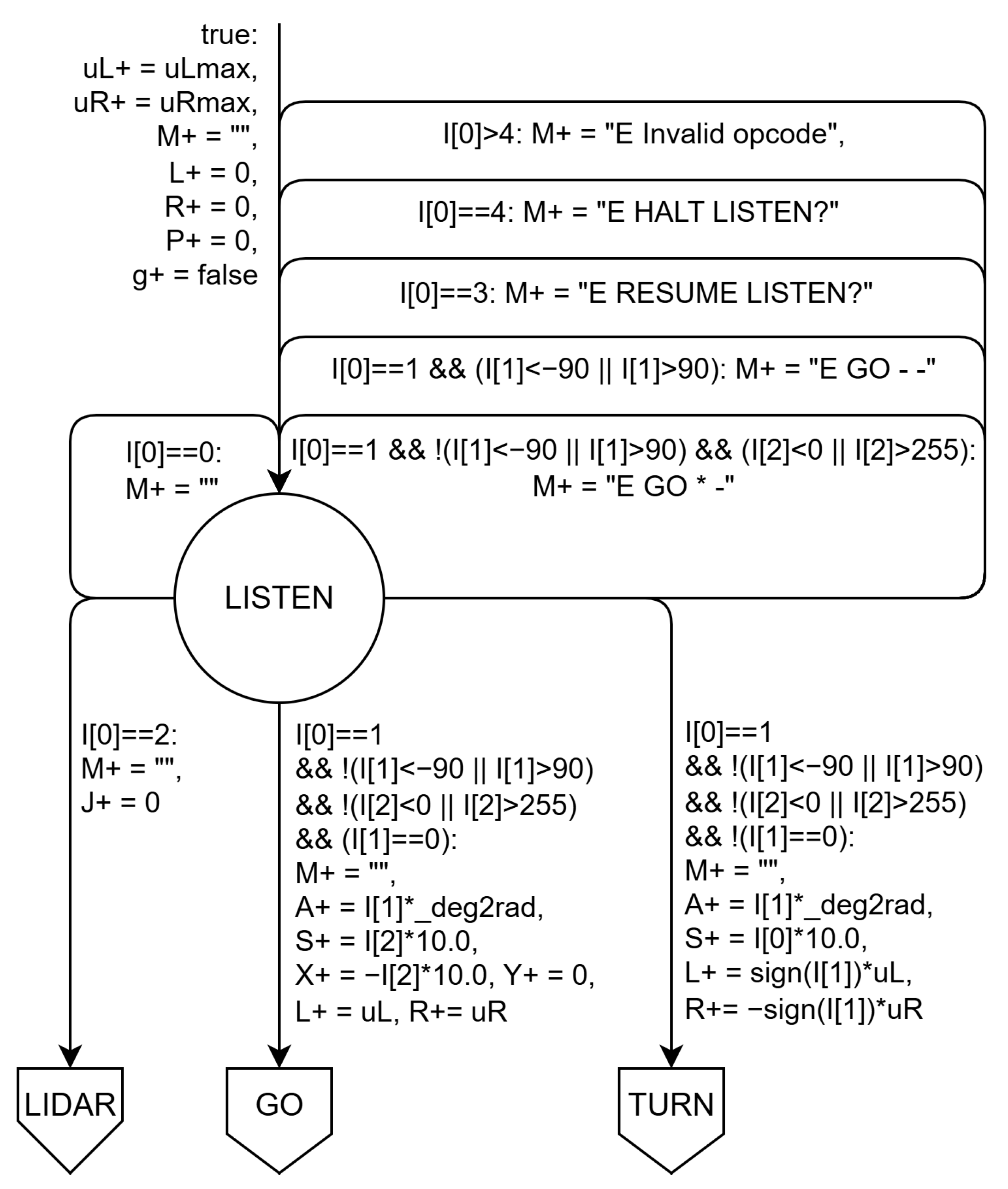
Figure 6.
Section of the L0Main controller EFSM for LIDAR sweep operations.
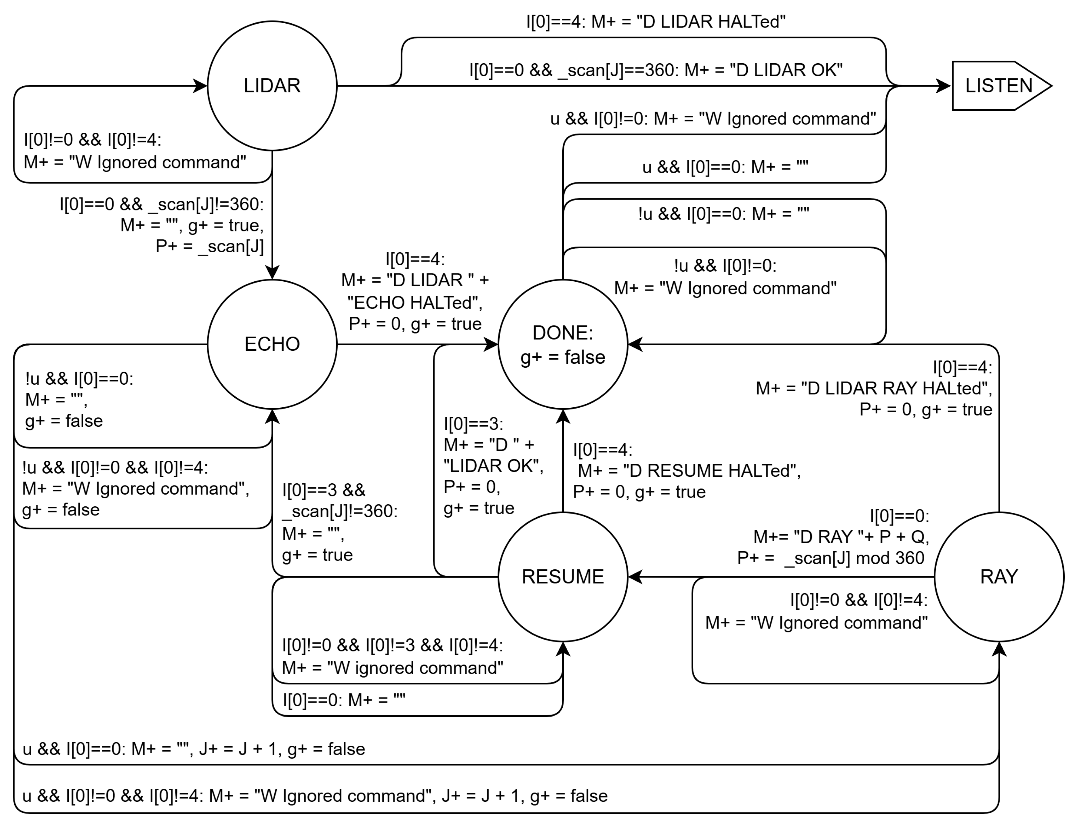
Figure 7.
Section of the L0Main controller EFSM for locomotion.
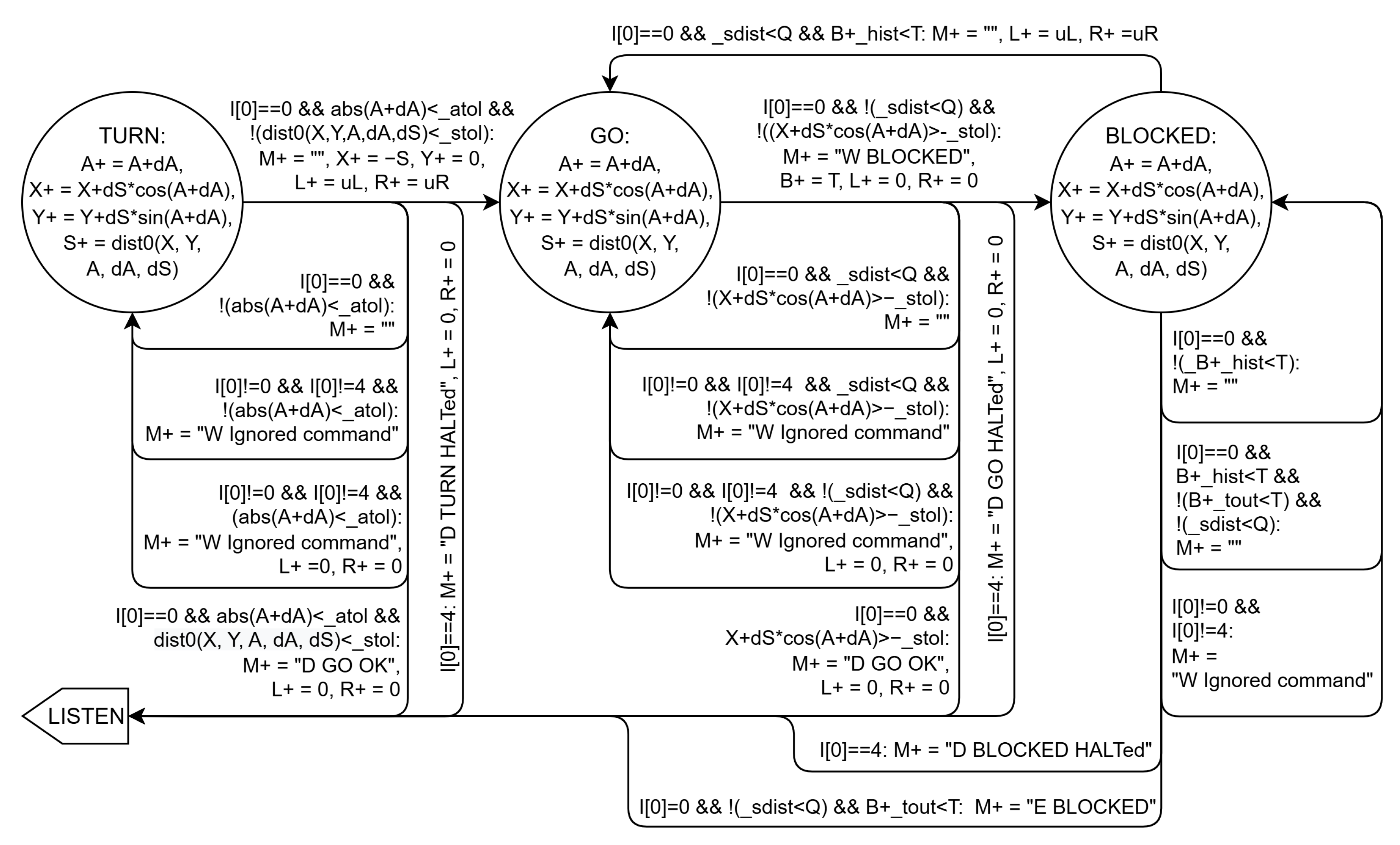
Figure 8.
Computation of yaw angle error from known position , orientation A, and variations in angle and linear displacement .
Figure 8.
Computation of yaw angle error from known position , orientation A, and variations in angle and linear displacement .
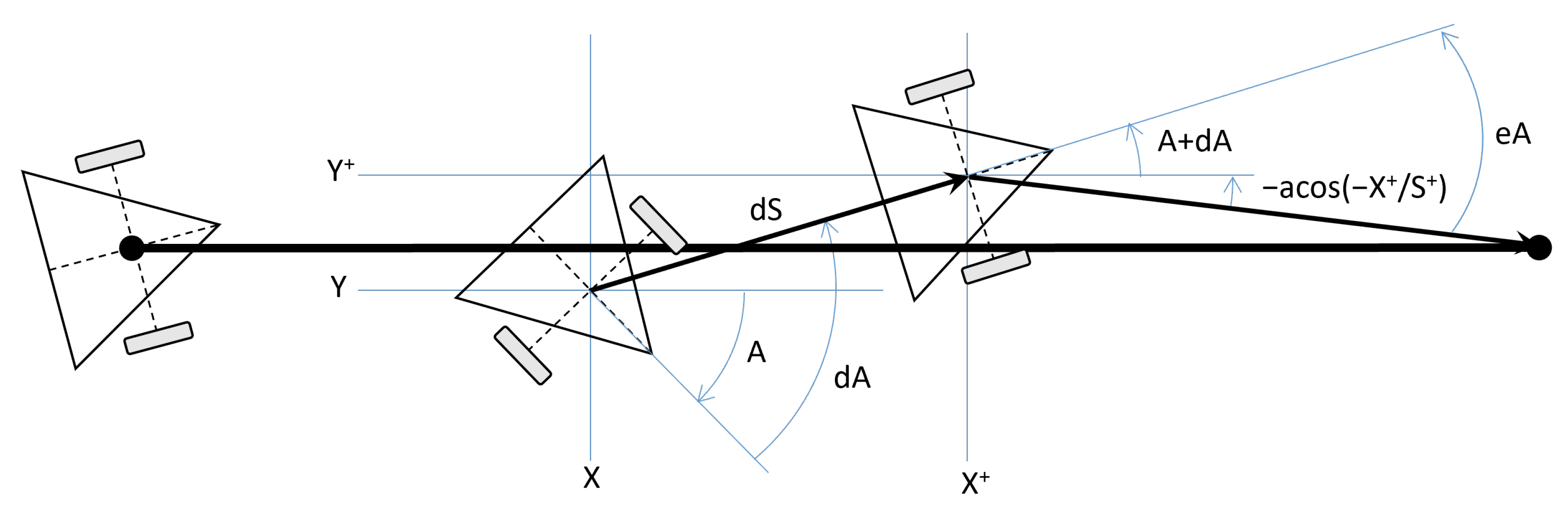
Figure 9.
Controller stack architecture, including a robot digital twin and L0L1Link interface layer to synchronize messages from virtual and real L0 levels.
Figure 9.
Controller stack architecture, including a robot digital twin and L0L1Link interface layer to synchronize messages from virtual and real L0 levels.
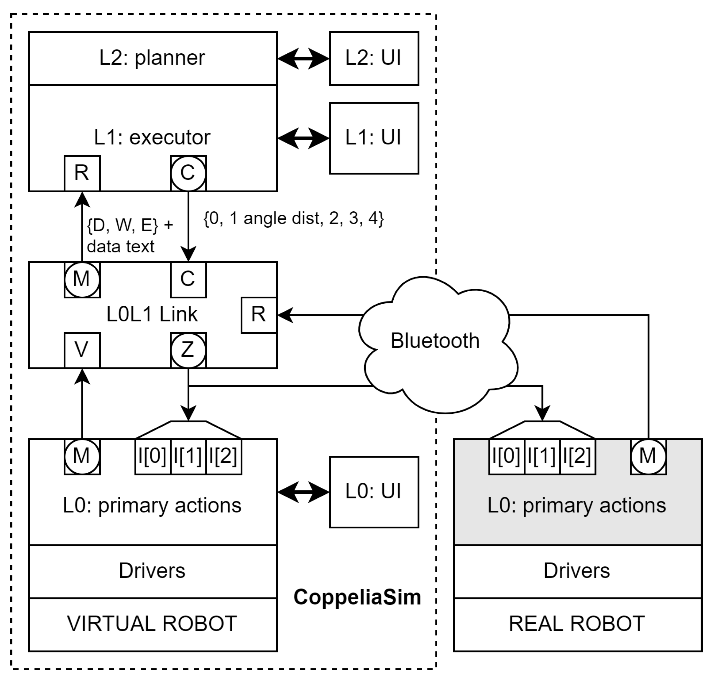
Figure 10.
EFSM execution model.
Disclaimer/Publisher’s Note: The statements, opinions and data contained in all publications are solely those of the individual author(s) and contributor(s) and not of MDPI and/or the editor(s). MDPI and/or the editor(s) disclaim responsibility for any injury to people or property resulting from any ideas, methods, instructions or products referred to in the content. |
© 2025 by the authors. Licensee MDPI, Basel, Switzerland. This article is an open access article distributed under the terms and conditions of the Creative Commons Attribution (CC BY) license (http://creativecommons.org/licenses/by/4.0/).
Copyright: This open access article is published under a Creative Commons CC BY 4.0 license, which permit the free download, distribution, and reuse, provided that the author and preprint are cited in any reuse.


