Submitted:
12 November 2025
Posted:
13 November 2025
You are already at the latest version
Abstract
The accurate prediction of the spatiotemporal evolution of rock damage zones is crucial for evaluating the stability of mine rock mass engineering. However, existing data-driven approaches often face challenges in effectively representing spatial heterogeneity and incorporating physical constraints, which can lead to predictions that deviate from mechanical laws. In this study, a physics-constrained spatio-temporal convolutional long short-term memory (STConvLSTM) network is proposed to address these limitations. First, a bidirectional point cloud–voxel adaptive conversion mechanism is designed to dynamically adjust voxel granularity according to point cloud density, thereby enhancing spatial detail preservation and computational efficiency. Second, a composite loss function combining structure-aware loss and physics-based constraints is constructed to ensure the predicted results satisfy mechanical continuity, smoothness, and boundary consistency. The proposed multi-level STConvLSTM integrates 3D convolution, CBAM3D attention, and residual connections to strengthen spatiotemporal feature extraction. Experimental results based on uniaxial compression–acoustic emission data demonstrate that the proposed method achieves an accuracy of 92.6% and an F1-score of 0.947, outperforming ConvLSTM and UNet3D models by 2.3% and 9.7%, respectively. These findings validate the effectiveness of the proposed framework in improving the physical reliability and predictive precision of rock damage evolution modeling.
Keywords:
rock damage prediction
; physics-constrained deep learning
; spatiotemporal modeling
; acoustic emission data
1. Introduction
Accurately predicting the spatiotemporal evolution of three-dimensional rock damage zones is fundamental for evaluating the long-term safety and durability of engineering structures. With the development of deep learning, data-driven approaches have shown strong potential in reducing prediction errors and improving computational efficiency. Meanwhile, advanced measurement techniques—such as LiDAR, synchrotron CT, and acoustic emission technology—provide a solid data foundation for high-precision modeling[1,2,3]. Recent studies have reported encouraging progress: deep models for surrounding-rock deformation in high-speed railway tunnels [4], hybrid constitutive modeling and deformation prediction for sandy limestone [5], transfer-learning-enhanced ConvLSTM for fracture evolution [6], LSTM-DCNN with transfer learning for mining-induced surface settlement [7], Newton–Raphson–BP for rockburst intensity [8], and CNN-LSTM under imbalanced data for rockburst grading [9]. For 3D structure learning from point clouds/voxels, VoxelNet and point–voxel fusion architectures have provided strong baselines [10,11,12].
However, key bottlenecks remain for 3D damage-zone forecasting. (1) Data representation vs. fidelity: damage point clouds are unstructured, sparse, and strongly heterogeneous; fixed-resolution voxelization easily loses details in critical areas, while pure point-based models (e.g., PointNet++) lack explicit temporal modeling [11,12]. Recent mixed point–voxel and sparse 3D backbones (PVCNN, submanifold sparse CNNs, Minkowski sparse ConvNets) markedly improve efficiency and fidelity on rock-like sparse geometries, motivating our density-adaptive voxelization design [13,14,15]. (2) Physics inconsistency: purely data-driven predictors can deviate from fracture mechanics if training data underrepresent governing constraints, as noted in physics-informed learning for geoscience and PINNs literature [16,17]. Beyond these, phase-field/PINN fracture studies show that embedding energy-based criteria (Griffith-type) into deep models improves mechanical plausibility, informing our physics-aware composite loss [18]. (3) Spatiotemporal modeling limits: standard ConvLSTM often relies on 2D convolutions and struggles with complex 3D topology. A 3D pathway remains essential—3D U-Net is a strong encoder–decoder baseline for volumetric context [19], and 3D-ConvLSTM has demonstrated superior forecasting of evolving volumetric structures in longitudinal medical data, motivating our 3D extension to rock-damage sequences [20].
To overcome these challenges, this study builds upon the acoustic-emission–based regional correlation imaging method proposed by Yao et al. [21] and their subsequent work on the regionalized structural evolution of rock damage [22].Using this technique, the initial state and the dynamic point-cloud sequences of three-dimensional rock damage zones during the uniaxial compression process can be efficiently obtained. Related advances in 3D AE tomography and anisotropy-aware AE localization further support reliable internal imaging/localization for rocks, consistent with our AE-based inputs [23,24]. Based on these high-quality spatiotemporal datasets, we propose a deep-learning-based framework for predicting the three-dimensional evolution of rock damage zones. Specifically as follows:
(1) An adaptive voxelization algorithm is designed to dynamically adjust voxel granularity according to point-cloud density, preserving structural details in dense regions while improving computational efficiency.
(2) A composite loss function that combines structural perception, physical constraints, and over-prediction penalties is introduced to guide the model toward physically consistent evolution patterns.
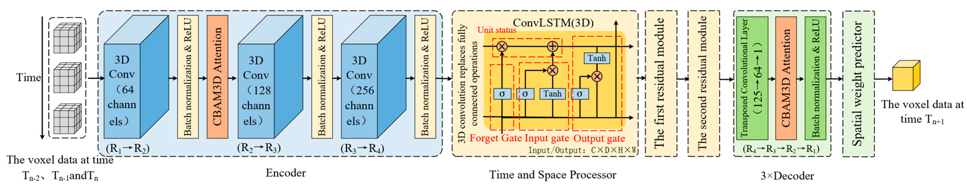
(3) A multi-level encoder–processor–decoder architecture of the spatiotemporal convolutional LSTM (STConvLSTM) network is developed, integrating 3D convolution and ConvLSTM to enhance joint spatiotemporal modeling capability. equipped with CBAM-style attention to enhance channel- and space-selective perception, 3D CBAM variants have proved effective in volumetric segmentation and motivate our attention design [25,26].
Through this coordinated design, the adaptive voxelization mechanism optimizes input representation, the STConvLSTM learns the temporal–spatial evolution laws, and the composite loss enforces physical and structural constraints, jointly improving predictive accuracy and physical credibility. Through laboratory uniaxial compression with synchronized AE acquisition, we validate that the proposed method achieves higher predictive accuracy and more realistic damage patterns than prevalent ConvLSTM/UNet variants, supporting its use for early-warning and support-design scenarios in underground engineering.
2. Materials and Methods
2.1. Data Source and Experimental Setup
A time-series dataset of three-dimensional damage evolution was obtained from uniaxial compression- acoustic emission tests on rock specimens (Figure 1). The cube specimens had an edge length of 100 mm. The measurements record the full process from initial damage to macroscopic failure over 18 time steps, and the raw data are stored on a 100 × 100 × 100 regular grid in “.mat” format. Damage regions were extracted from the velocity field using the fuzzy C-means (FCM) algorithm and converted into sequences of 3D point clouds (each record contains the velocity value and the corresponding XYZ coordinates). This dataset exhibits pronounced spatial heterogeneity and temporal evolution, making it suitable for evaluating the proposed method’s capabilities in representation, spatiotemporal modeling, and physical consistency.

Scheme 1.
Experimental setup.
| Hyperparameter | Value/Setting | Purpose |
| Voxel resolution | 100×100×100 | Preserve spatial detail features |
| Input time step (sliding window) | 2 | Capture the recent evolutionary history |
| Prediction time step | 1 | Evaluate the accuracy of single-step predictions |
| Learning rate scheduling strategy | Cosine annealing | Stabilize and converge to the optimal solution |
| Optimizer | AdamW | Improve training stability |
Composite loss weight  、 、 、 、
|
Balance various optimization objectives |
2.2. Methods Procedures and Adaptive Voxelization
Pipeline steps are as follows: First, the global range of the dataset is analyzed, and the raw point-cloud data are feature-normalized using a MinMaxScaler. Subsequently, temporal samples are constructed through a sliding-window mechanism. During the data-loading stage, adaptive voxelization based on K-nearest neighbor (KNN) density estimation accelerated by a KD-tree is performed on each time-step normalized point cloud to generate multi-resolution voxel representations. The encoder–processor–decoder STConvLSTM network with integrated CBAM3D attention modules is then employed for spatiotemporal modeling and prediction, while model parameters are optimized through a composite loss function combining structural perception loss and physical constraint loss. Finally, the predicted voxel fields are thresholded and con-verted back into point clouds, followed by inverse normalization to complete recon-struction and visualization evaluation.
This workflow, illustrated in Figure 2, achieves an end-to-end learning framework that synergistically integrates adaptive data representation, spatiotemporal modeling, and physical constraints, thereby substantially improving prediction accuracy while ensuring physical consistency.
To enable efficient learning on regular grids while preserving critical structures, point clouds were converted to voxels via a bidirectional adaptive point-cloud–voxel conversion mechanism. Local voxel granularity is dynamically adjusted according to point density: finer voxels are assigned to dense, structure-critical zones (detail preservation), whereas coarser voxels are used in sparse areas (efficiency). Figure 3 shows the adaptive voxelization process.
2.3. Physics-Constrained STConvLSTM Architecture
The network follows an encoder–processor–decoder design.
Encoder: three cascaded 3D convolutional blocks (3×3×3 kernels) with batch normalization and ReLU progressively downsample inputs into compact feature maps while increasing channels. A CBAM3D module (channel + spatial attention) is integrated after the initial feature extractor to enhance sensitivity to damage-relevant structures. Let the input voxel tensor be ,The output of the layer () in the encoder is computed as follows:
Where (input initialization), and denotes the 3D convolution layer of the -th level with a kernel size of 3×3×3 and a stride n, which can be adjusted according to the dataset scale. In addition, the CBAM3D module in Equation (1) is further decomposed into two sequential steps—channel attention and spatial attention—as expressed by:
Here, performs global pooling on followed by weighting through a multilayer perceptron (MLP), producing channel-attention weights that are multiplied with the input features. This mechanism mimics the human visual system’s selective attention to different feature channels, enabling the network to adaptively emphasize the channels relevant to rock-damage evolution while suppressing irrelevant or noisy ones. then applies spatial pooling and a 7×7×7 convolution to the channel-weighted features, generating spatial-attention weights that emphasize important spatial locations. The large convolution kernel ensures a broad receptive field, effectively capturing contextual information of key structural regions in the rock-damage domain and guiding the model to focus on these spatially critical areas. Finally, serves as the input to the next layer, completing the effective integration of feature extraction and attention enhancement.
Spatiotemporal processor: a 3D ConvLSTM core replaces fully connected mappings with 3D convolutions in the gate transitions, enabling joint modeling in space and time and retaining path dependence of damage evolution.
Decoder: three transposed-convolution blocks (with batch normalization, ReLU, and CBAM3D) progressively restore resolution and produce the predicted damage field. The output feature of decoder can be expressed as:
Where denotes the output of the layer, and represents the 3D transposed convolution operation. To stabilize gradients and strengthen feature reuse, dual residual connections are adopted around the ConvLSTM outputs and subsequent nonlinear transforms; a lightweight spatial weighting predictor further emphasizes key regions and suppresses over-prediction at noncritical locations. The network structure is as follows:
Figure 4.
Network structure.
2.4. Composite Loss with Physical Constraints
The total objective combines a structure-aware term, a physics-constraint term, and an over-prediction penalty:
Structure-aware loss prioritizes geometric fidelity at crack boundaries and preserves morphological continuity.
Where represents the adaptive weight, which enables the model to pay more attention to the areas that are difficult to predict. maintains the structural regularity of the prediction.
The design of the physical constraint loss not only considers the spatial continuity and smoothness of the predicted results, but also incorporates the classical theories of rock mechanics. Specifically, the mathematical formulation of the continuity and smoothness constraints can be analogized to the Griffith energy criterion . By constraining the spatial variation of the damage zone, the model indirectly regulates the energy release process during damage evolution. The edge-distribution constraint draws on the physical meaning of the stress intensity factor, which suppresses abnormal distributions along the damage-zone boundaries and prevents the occurrence of local stress concentration. Furthermore, the weighted combination of all the loss components reflects the multi-field coupling characteristics of rock materials during deformation and fracture, ensuring that the prediction results are more consistent with the actual physical mechanisms of rock failure. Based on the Griffith energy criterion, the spatial distribution of the damage zone is represented by a voxel field , whose spatial variation can be approximated using finite-difference gradients as follows:
The physical constraint loss consists of three core components, ensuring that the predicted results conform to rock-mechanical principles:
Where, denotes the expectation over all voxels, is an indicator function, and is a threshold parameter. The continuity constraint ensures that the damage region varies continuously in space, preventing the appearance of abrupt or disconnected zones. The smoothness constraint controls curvature variation, avoiding unnatural sharp bending, while the edge-distribution constraint regulates the boundary characteristics to prevent overly concentrated or dispersed edge distributions.
Over-prediction penalty uses the ReLU function to implement a one-sided penalty that is activated only when the predicted damage volume exceeds the true volume. The penalty intensity increases linearly with the degree of over-prediction.
The composite loss function maintains high prediction accuracy while significantly improving the physical rationality and practical reliability of the results.
2.5. Training Protocol and Evaluation Metrics
Model training uses a sliding window of two historical time steps to predict the next time step. Performance is assessed with Accuracy, Recall, F1-score (harmonic mean of Accuracy and Recall), and Point-Cloud Coverage (PC-Coverage), which quantifies the proportion of true damaged points covered by the predicted point cloud. These metrics jointly evaluate reliability (Accuracy), detection ability (Recall), balanced performance (F1), and spatial completeness (PC-Coverage).
Comparative studies against 3D CNN, ConvLSTM, and UNet3D are reported in the Results section, together with ablation experiments isolating the contributions of adaptive voxelization and the composite loss.
Where TP denotes the number of true positives, FP is the number of false positives, and FN is the number of false negatives.
3. Results
3.1. Visualization of Damage Evolution
Visualization serves as a key diagnostic to assess the model’s ability to capture spatial structures, temporal evolution, and mechanical consistency. Figure 5 presents eight consecutive stages of the clustered three-dimensional damage region corresponding to the damage core zone. As loading and stress increase, the damage area gradually expands in both size and morphological complexity, exhibiting branching and merging phenomena—characteristics consistent with physical damage accumulation processes.
3.2. Single-Step Prediction and Spatial Fidelity
A direct comparison between the true and predicted point clouds at one representative time step (Figure 6) demonstrates the high fidelity of the proposed STConvLSTM model. The overall structural similarity exceeds 90 %, and the predicted accuracy reaches 92.6 %, confirming that the model effectively reconstructs both the shape and extension trend of the actual damage zone.
Discrepancies, highlighted by red boxes in Figure 6, mainly occur near multi-damage intersections or along the damage boundaries—regions of high stress concentration and nonlinear deformation. This observation aligns with the known degradation of predictive accuracy in multi-damage interference zones, where local stress superposition and fracture bifurcation produce complex evolution paths.
3.3. Error Distribution Analysis
To further quantify prediction reliability, the spatial distribution of errors between the predicted and real data was analyzed (Figure 7). Most regions, especially the damage core, display low residuals close to zero, reflecting high overall accuracy and consistency with experimental data. The predicted results achieve an accuracy of 0.926, F1 = 0.950, and point-cloud coverage = 0.975, indicating that nearly the entire damaged volume is captured. The structural similarity index (SSIM = 0.884) also supports excellent agreement in spatial topology.
Higher errors at boundary areas result from temporal uncertainty propagation in multi-path evolution: although fine voxelization alleviates this issue, the temporal model tends to output conservative, probabilistic boundary predictions, leading to slight overestimation of the damaged extent
3.4. Cross-Sectional Validation
To visualize local prediction quality, cross-sections of error distribution at specific coordinates (X = 1, 21; Y = 1, 21; Z = 21, 41) were analyzed within the 100 × 100 × 100 voxel space (Figure 8). Most regions exhibit blue–green low-error zones, consistent with the high global similarity reported above. Red–yellow patches, representing larger deviations, appear mainly near complex geometric boundaries, implying potential improvement space for future boundary-refinement modules.
3.5. Temporal-Step Prediction Verification
The model was also tested for multi-step temporal reasoning: using two historical time frames (t − 1, t) to predict the next one (t + 1). As shown in Figure 9, the predicted expansion trend matches the pattern observed in prior steps, with a spatial structure similarity exceeding 90 %. Even without direct ground-truth comparison at this step, the consistency of propagation confirms that the model has learned stable spatiotemporal dynamics rather than memorizing static frames.
3.6. Comparative Study with Baseline Models
To evaluate overall performance, STConvLSTM was compared against 3D CNN, ConvLSTM, and UNet3D baselines (Table 2). STConvLSTM achieved the highest accuracy (0.926) and F1-score (0.950), while maintaining competitive recall and coverage (0.975 each). ConvLSTM slightly exceeded STConvLSTM in recall due to its tendency to over-predict damaged zones, but this comes at the cost of precision. The results demonstrate that the proposed physics-constrained model effectively balances recall and precision, improving both numerical accuracy and physical plausibility of the predicted evolution (Table 2).
3.7. Ablation Experiments
Ablation tests (Table 3) were designed to quantify the contributions of key modules:
1.removing adaptive voxelization (fixed voxels + composite loss);
2.replacing the composite loss with simple MSE (adaptive voxels + MSE only);
3.the complete model.
The complete model achieves the highest values in accuracy and F1-score.Compared with the “MSE-only” model, the accuracy increases by 8.3% and the F1-score by 4.5%; compared with the “fixed-voxel” model, the accuracy increases by 6.5% and the F1-score by 2.4%.The recall and point-cloud coverage of the complete model are lower than those of the simplified models (fixed voxels / MSE only). This reflects an over-prediction tendency in the simplified models: they tend to predict a larger damaged area, which yields higher recall and point-cloud coverage but sacrifices precision. The ablation experiments confirm that removing the composite loss leads to a substantial drop in physical rationality and accuracy-related metrics; this module is key to improving physical plausibility and predictive accuracy. Removing adaptive voxelization causes detail loss and introduces redundant computation in sparse regions. The results show that this module further refines fine-grained representation and improves computational efficiency. Together, the two modules act synergistically to deliver the best performance (Table 3).
The experimental findings confirm that incorporating physics-based constraints within a deep spatiotemporal framework can significantly improve both the accuracy and interpretability of rock damage prediction. Adaptive voxelization resolves the scale-precision dilemma, and the physics-aware composite loss aligns model outputs with established fracture-mechanics principles. Although residual errors remain near complex boundaries, the results highlight the method’s robustness for damage early-warning and long-term stability evaluation in underground mining and geotechnical engineering. Future work will focus on enhancing fine-scale boundary modeling and integrating multi-physics coupling effects for even greater predictive reliability
4. Discussion
Performance in context: Compared with 3D CNN, ConvLSTM and UNet3D baselines, the proposed physics-constrained STConvLSTM achieves the best Accuracy (0.926) and F1 (0.950), while maintaining competitive Recall/PC-Coverage (0.975); ConvLSTM’s slight Recall advantage stems from over-prediction, traded off against precision. These observations support that physics-aware regularization improves precision without sacrificing detectability. They are reinforced by our ablation tests showing that removing the composite loss or adaptive voxelization degrades accuracy/F1 or detail retention, respectively, confirming the necessity of both modules.
Representation matters: Damage point clouds are sparse and heterogeneous; fixed-resolution voxelization loses critical details. Our density-adaptive point-cloud↔voxel conversion preserves fine structures in dense regions while keeping computation tractable, forming an effective interface to volumetric learners. This design choice is consistent with evidence that point–voxel fusion and sparse 3D convolutions (PVCNN, Submanifold SparseConv, Minkowski) enhance efficiency and fidelity in sparse 3D fields [13,14,15]. Together with a 3D encoder–decoder pathway—a proven volumetric baseline typified by 3D U-Net—it provides the spatial context standard ConvLSTM lacks [19].
Physics guidance as a regularizer: Purely data-driven models can drift from mechanics, yielding torn or over-diffuse fronts [16,17]. Our composite loss introduces (i) continuity and smoothness terms (Griffith-motivated) and (ii) an edge-distribution constraint related to the stress-intensity factor, plus (iii) a one-sided over-prediction penalty. Collectively these steer predictions toward mechanically admissible morphologies and curb non-physical expansion. This approach aligns with theory-guided learning and recent phase-field/PINN fracture studies that embed energy consistency to improve plausibility [18].
Error anatomy and boundary behavior: Residuals cluster at multi-damage interference zones and along complex boundaries—regions of high stress concentration and multi-path evolution—precisely where temporal uncertainty propagates and models tend to output conservative, probabilistic fronts. Cross-sectional views confirm low error in cores but larger deviations near intricate geometries, indicating room for boundary-refinement modules.
Implications for practice: Given the strong Accuracy/F1 and physically consistent morphologies, the method is well suited to early-warning and support-design scenarios in underground engineering, provided domain calibration is performed. This aligns with emerging multi-sensor early-warning frameworks (MS–AE–EMR) where deep learning improves risk assessment timeliness [27], and with the broader thrust of theory-guided data science in geomechanics [17].
Limitations and future directions: (1) Boundary refinement via curvature-aware or energy-aware regularization (e.g., boundary/phase-field surrogates) to reduce local errors; (2) stronger volumetric saliency using boundary-focused attention; (3) multi-physics coupling (e.g., fusing AE with ultrasonic velocity/IR fields) to better constrain edge behavior under high stress gradients; (4) broader validation across lithologies, loading paths, and field heterogeneity for deployment readiness [18,27,28]. Our experiments and error maps suggest these steps are the most impactful next moves.
5. Conclusions
This study proposed a physics-constrained deep-learning framework for predicting the spatiotemporal evolution of three-dimensional rock damage zones. The model demonstrates superior accuracy, physical consistency, and generalization compared with conventional data-driven methods, providing a promising approach for intelligent rock-mass stability assessment. The main findings are summarized as follows:
(1) A bidirectional adaptive voxelization algorithm was developed to dynamically adjust voxel granularity based on local point-cloud density. This design preserves key structural details in dense core regions while enhancing efficiency in sparse zones, effectively balancing computational cost and representation precision.
(2) A hierarchical encoder–processor–decoder architecture integrating 3D convolution, CBAM3D attention, and residual connections was constructed. The model substantially strengthens joint spatiotemporal feature learning and overcomes the weak spatial perception and limited temporal modeling of conventional ConvLSTM-based networks.
(3) The introduction of a multi-objective loss combining structural perception, physics constraint, and over-prediction penalty improves both physical plausibility and predictive precision. It suppresses non-physical divergence, mitigates boundary artifacts, and enhances the model’s ability to generalize under complex loading conditions.
Overall, the proposed framework achieves an accuracy of 0.926 and an F1-score of 0.947 on the rock damage dataset, clearly outperforming baseline models. The method provides an efficient and reliable computational paradigm for early warning of rock failure, structural integrity monitoring, and deep-mining safety evaluation. Future work will focus on improving the model’s capability to handle complex boundary conditions and incorporating coupled thermo–hydro–mechanical effects to extend its applicability to broader geological environments
Author Contributions
S.Y.: Writing—original draft, Investigation, Visualization, Formal analysis, Data curation, Funding acquisition. Z.T.: Review—editing, Methodology, Investigation, Visualization, Formal analysis, Supervision. Y.Z.: Review—editing, Supervision, Funding acquisition. X.Y.: Review—editing, Supervision, Funding acquisition. ZG.T.: Review—editing, Visualization. S.W.: Review—editing, Visualization. All authors have read and agreed to the published version of the manuscript.
Funding
This study was supported by the National Natural Science Foundation of China (Grant No. 52474099)
Data Availability Statement
The original contributions presented in the study are included in the article. Further inquiries can be directed to the corresponding author.
Conflicts of Interest
The authors declare no conflicts of interest.
References
- Jiang, L.X.; Liu, Y.; Wang, C.; et al. In-situ micro-CT damage analysis of carbon and carbon/glass hybrid laminates under tensile loading by image reconstruction and DVC technology. Composites Part A: Applied Science and Manufacturing 2024, 176, 107822. [Google Scholar] [CrossRef]
- Wang, Y.; Tian, X.B.; Xu, H.Z.; et al. Joint inversion of gravity and gravity gradient for 3D density structure of lithosphere in Tibetan Plateau and adjacent areas. Chinese Journal of Geophysics 2017, 60, 2469–2479. [Google Scholar] [CrossRef]
- Ke, X.P.; Wang, Y.; Xu, H.Z.; et al. Gravity inversion of 3D crustal density structure in Tibetan Plateau. Progress in Geophysics 2009, 24, 448–455. [Google Scholar]
- Yang, Z.; Cheng, Z.; Wu, D. Deep learning driven prediction and comparative study of surrounding rock deformation in high speed railway tunnels. Scientific Reports 2025, 15, 24104. [Google Scholar] [CrossRef] [PubMed]
- Zhang, J.; Li, S.; Zhu, Q.; et al. Long-term and short-term constitutive model of rock based on deep learning and deformation prediction of sandy limestone. Rock and Soil Mechanics 2025, 46, 289–302. [Google Scholar] [CrossRef]
- Liu, R.Z.; Wang, Z.W.; Zhang, Y.B.; et al. Research on rock fracture evolution prediction model based on Adam-ConvLSTM and transfer learning. Discover Applied Sciences 2025, 7, 217. [Google Scholar] [CrossRef]
- Zhang, D.; Zhang, Y.; Jiao, S.; et al. Prediction Method for Surface Settlement during Underground Mining in Mines Based on LSTM-DCNN and Transfer Learning. Mining Research and Development 2025, 1–9. [Google Scholar] [CrossRef]
- Li, J.; Wang, Y.; Zhang, T.; et al. Rockburst Intensity Prediction Model Based on Newton–Raphson Algorithm and BP Neural Network. Mining Research and Development 2025, 45, 127–133. [Google Scholar] [CrossRef]
- Zheng, L.; Liang, P.; Li, G.; et al. CNN-LSTM Rockburst Intensity Grade Prediction Model Based on Fusion Optimization Algorithm under Unbalanced Data. Mining Research and Development 2025, 45, 111–118. [Google Scholar] [CrossRef]
- Zhou, Y.; Tuzel, O. VoxelNet: End-to-End Learning for Point Cloud-Based 3D Object Detection. In Proceedings of the IEEE Conference on Computer Vision and Pattern Recognition (CVPR); 2018; pp. 4490–4499. [Google Scholar] [CrossRef]
- Qi, C.R.; Yi, L.; Su, H.; et al. PointNet++: Deep hierarchical feature learning on point sets. In Advances in Neural Information Processing Systems (NeurIPS); 2017; pp. 5105–5114. arXiv:1706.02413.
- Wang, J.; Shi, S.; Zhang, G.; et al. PVLF: Point–Voxel Local Feature Fusion for 3D Detection. In Proceedings of the IEEE/CVF CVPR Workshops; 2023; pp. 4567–4576. [Google Scholar] [CrossRef]
- Liu, Z.; Tang, H.; Lin, Y.; Han, S. Point–Voxel CNN for Efficient 3D Deep Learning. Advances in Neural Information Processing Systems (NeurIPS), 1907. [Google Scholar]
- Graham, B.; van der Maaten, L. Submanifold Sparse Convolutional Networks. Proceedings of the IEEE Conference on Computer Vision and Pattern Recognition (CVPR), 1706. [Google Scholar]
- Choy, C.; Gwak, J.; Savarese, S. 4D Spatio-Temporal ConvNets: Minkowski Convolutional Neural Networks. In Proceedings of the IEEE Conference on Computer Vision and Pattern Recognition (CVPR); 2019. [Google Scholar] [CrossRef]
- Raissi, M.; Perdikaris, P.; Karniadakis, G.E. Physics-informed neural networks. Journal of Computational Physics 2019, 378, 686–707. [Google Scholar] [CrossRef]
- Karpatne, A.; Watkins, W.; Read, J.; et al. Theory-guided data science for geoscience. IEEE Transactions on Knowledge and Data Engineering 2022, 34, 3924–3938. [Google Scholar]
- Manav, M.; Molinaro, R.; Mishra, S.; De Lorenzis, L. Phase-field modeling of fracture with physics-informed deep learning. Computer Methods in Applied Mechanics and Engineering 2024, 429, 117104. [Google Scholar] [CrossRef]
- Çiçek, Ö.; Abdulkadir, A.; Lienkamp, S.S.; Brox, T.; Ronneberger, O. 3D U-Net: Learning dense volumetric segmentation from sparse annotation. In Medical Image Computing and Computer-Assisted Intervention (MICCAI); 2016; LNCS 9901, pp. 424–432. [CrossRef]
- Zhang, L.; Lu, L.; Wang, X.; Zhu, R.M.; Bagheri, M.; Summers, R.M.; Yao, J. Spatio-Temporal ConvLSTMs for Tumor Growth Prediction by Learning 4D Longitudinal Patient Data. arXiv 2019, arXiv:1902.08716. [Google Scholar]
- Yao, X.; Zhang, Y.; Sun, L.; et al. Research on Rock Damage Acoustic Emission Detection and Imaging Method Based on Regional Correlation. Chinese Journal of Rock Mechanics and Engineering 2017, 36, 2113–2123. [Google Scholar] [CrossRef]
- Yao, X.L.; Liu, Z.; Zhang, Y.B.; et al. Effect of regionalized structures on rock fracture process. Scientific Reports 2024, 14, 10490. [Google Scholar] [CrossRef] [PubMed]
- Cheng, Y.; Hagan, P.; Mitra, R.; Wang, S.; Yang, H.-W. Experimental investigation of progressive failure using 3D acoustic emission tomography. Frontiers in Earth Science 2021, 9, 765030. [Google Scholar] [CrossRef]
- Song, T.; Zhou, Y.; Yu, X. Three-Dimensional AE Source Localization for Layered Rock Considering Anisotropic P-Wave Velocity. Bulletin of Engineering Geology and the Environment 2024, 83, 185. [Google Scholar] [CrossRef]
- Woo, S.; Park, J.; Lee, J.-Y.; Kweon, I.S. CBAM: Convolutional Block Attention Module. In Proceedings of the European Conference on Computer Vision (ECCV); 2018. [Google Scholar] [CrossRef]
- Wang, J.; Yu, Z.; Luan, Z.; Ren, J.; Zhao, Y.; Yu, G. RDAU-Net: Residual CNN with DFP and CBAM for Brain Tumor Segmentation. Frontiers in Oncology 2022, 12, 805263. [Google Scholar] [CrossRef] [PubMed]
- Di, Y.; Wang, E.; Li, Z.; Liu, X.; et al. Comprehensive early warning of rockburst from MS–AE–EMR signals via deep learning. International Journal of Rock Mechanics and Mining Sciences 2023, 170, 105519. [Google Scholar] [CrossRef]
- Kervadec, H.; Bouchtiba, J.; Desrosiers, C.; Granger, E.; Dolz, J.; Ben Ayed, I. Boundary loss for highly unbalanced segmentation. Medical Image Analysis 2021, 67, 101851. [Google Scholar] [CrossRef] [PubMed]
Figure 1.
(a) The cracked specimen, (b) The 3D-Imaging at the moment before.
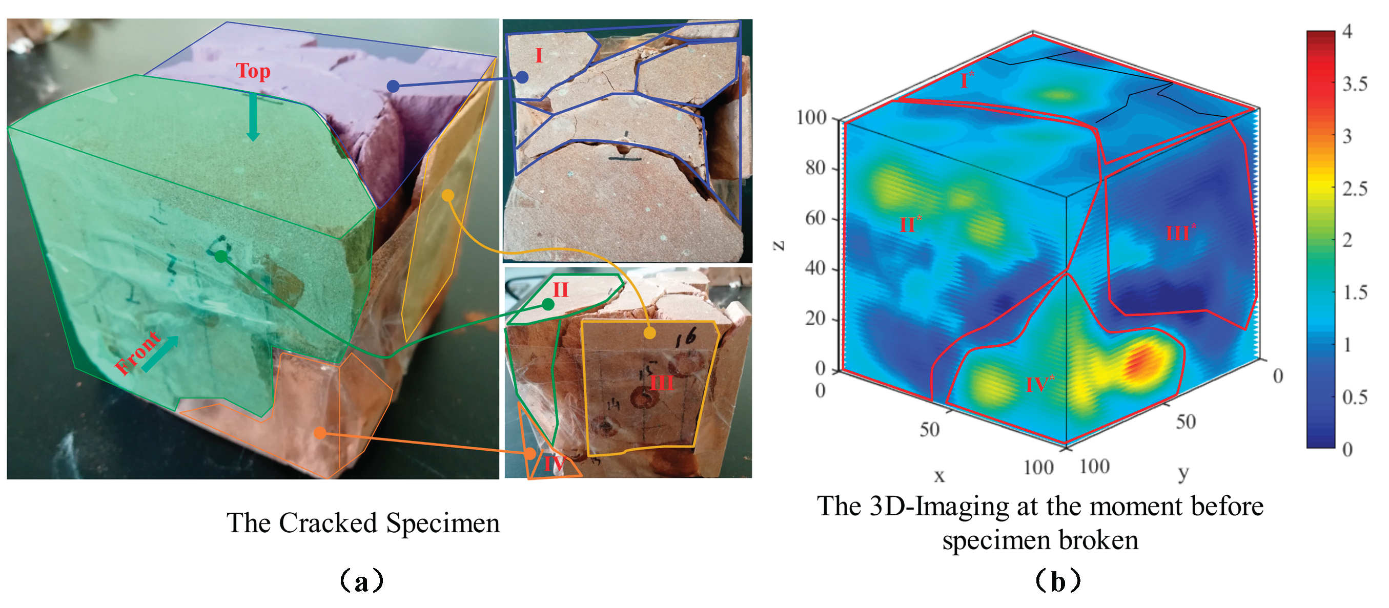
Figure 2.
Methods procedures.
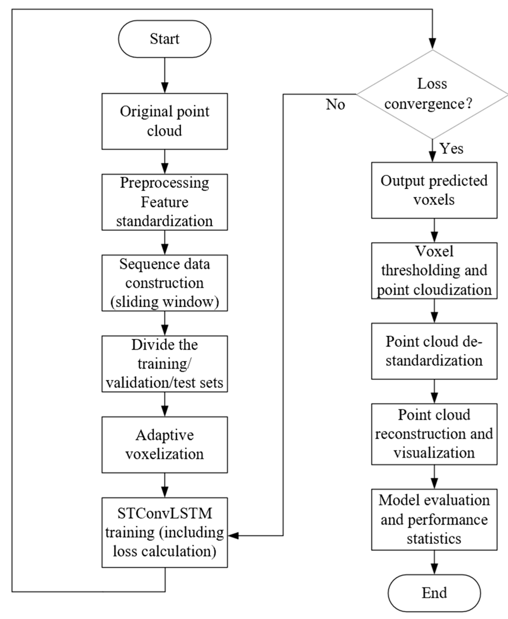
Figure 3.
Adaptive voxelization process, (a) Original point cloud data, (b) Point cloud density heat map, (c) Adaptive voxelization result, (d) Comparison of Point Clouds and Voxel Data.
Figure 3.
Adaptive voxelization process, (a) Original point cloud data, (b) Point cloud density heat map, (c) Adaptive voxelization result, (d) Comparison of Point Clouds and Voxel Data.
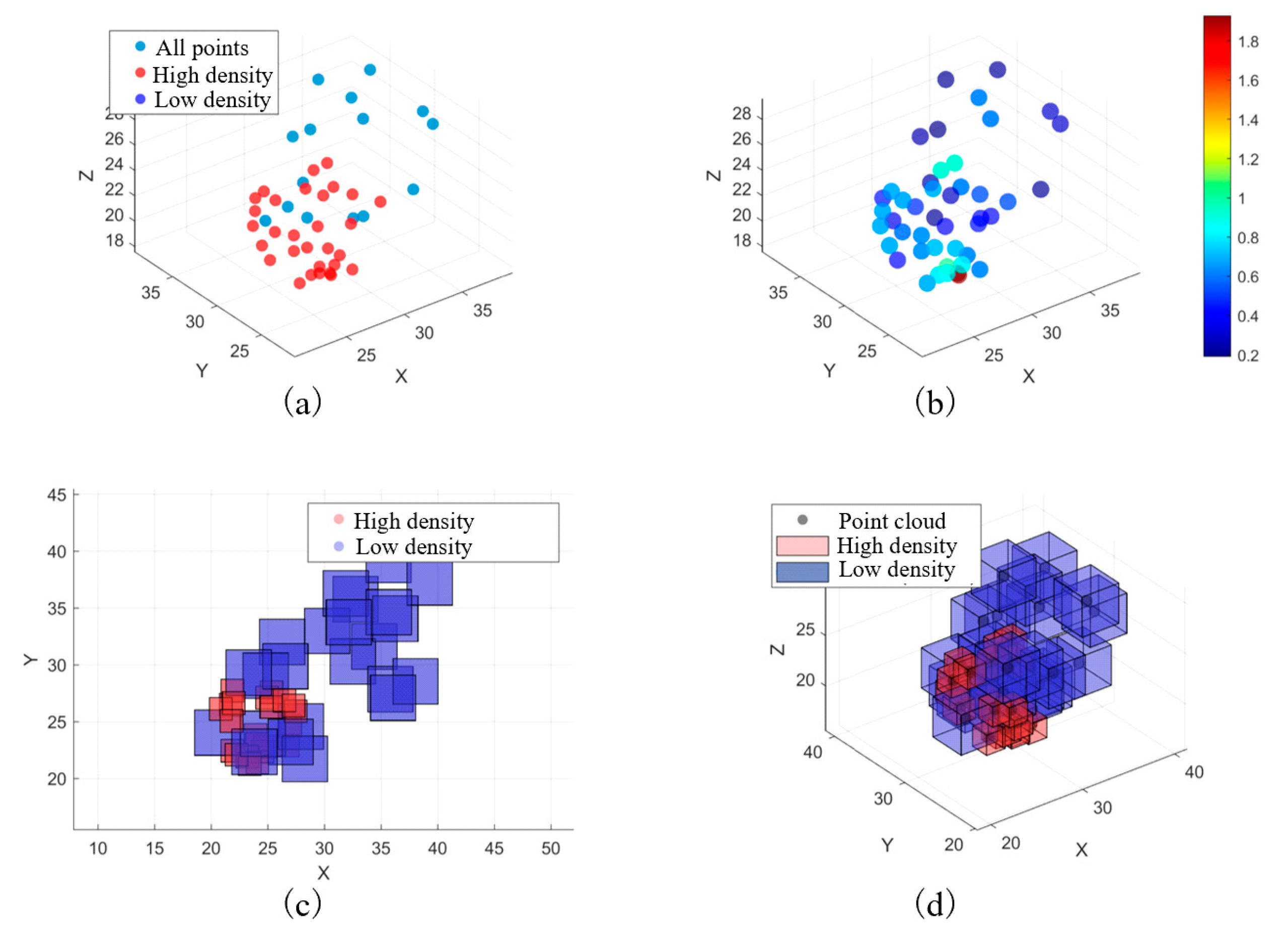
Figure 5.
Eight consecutive stages.
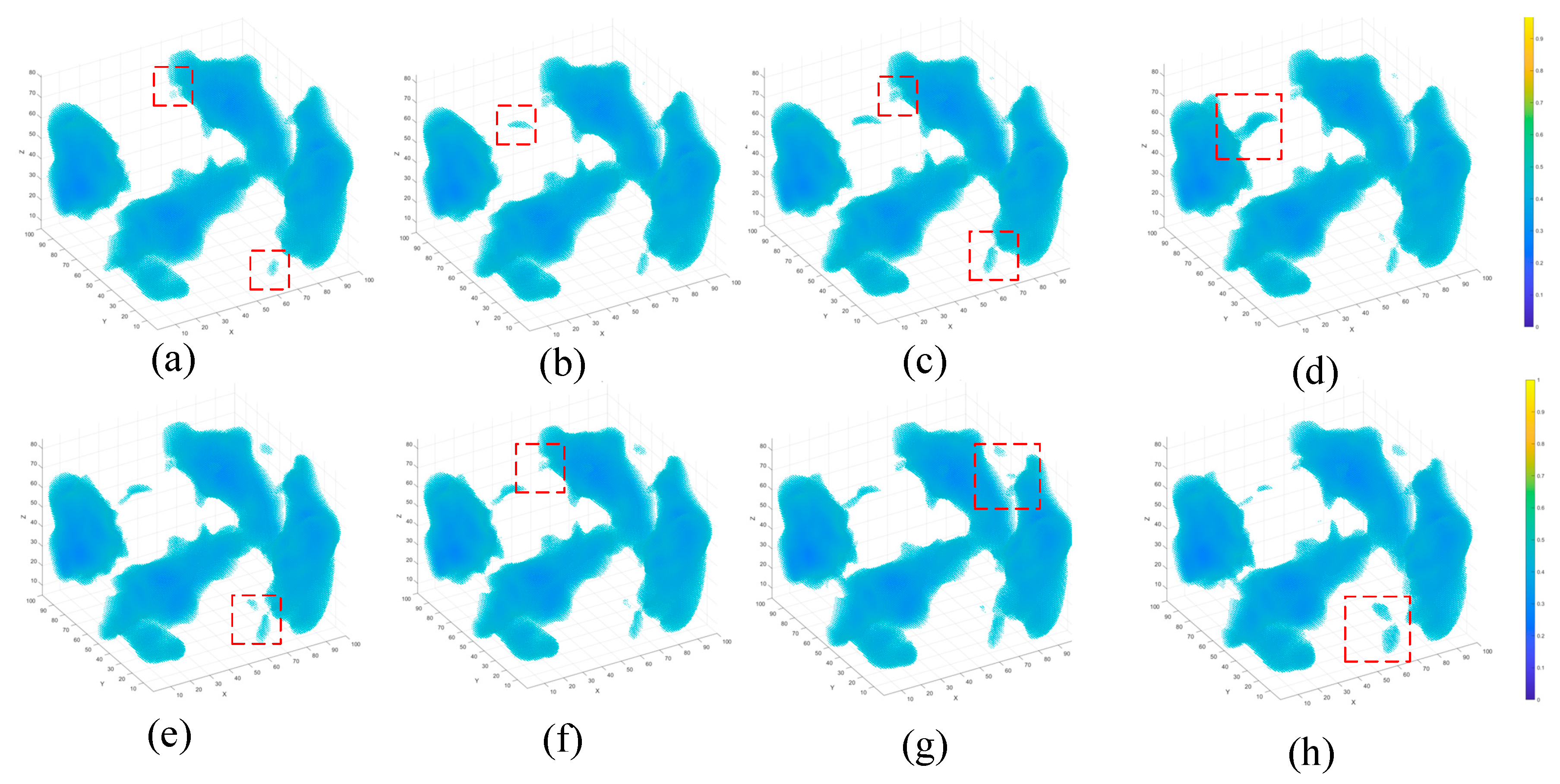
Figure 6.
Comparison diagram, (a) Real point cloud, (b) Predicted point cloud.
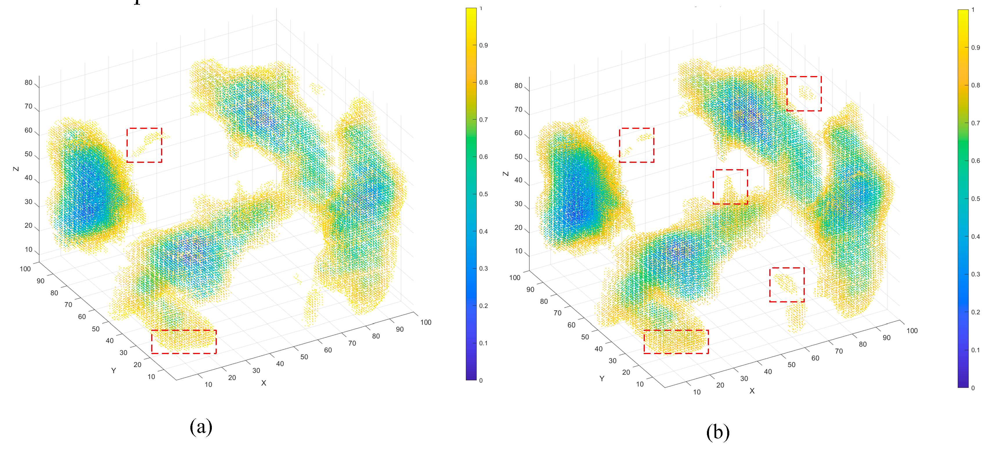
Figure 7.
Relative error distribution, (a) Front view, (b) Perspective view after rotation by 180 degrees.
Figure 7.
Relative error distribution, (a) Front view, (b) Perspective view after rotation by 180 degrees.
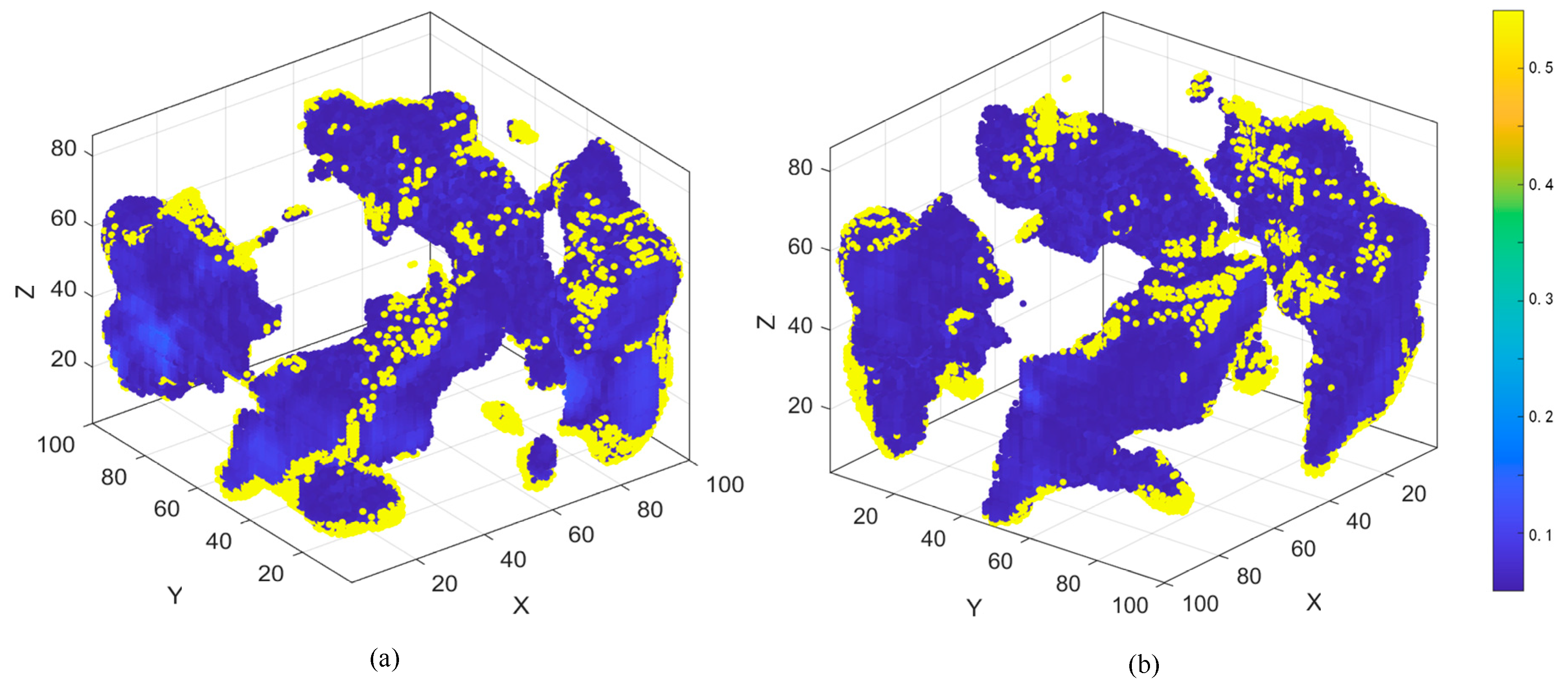
Figure 8.
Error distribution cross-sectional chart.
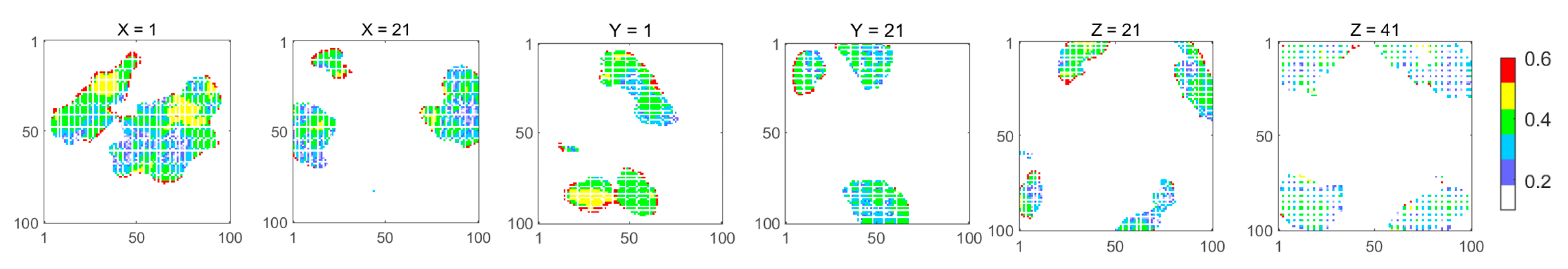
Figure 9.
Verification, two time steps ahead predict the next time step.
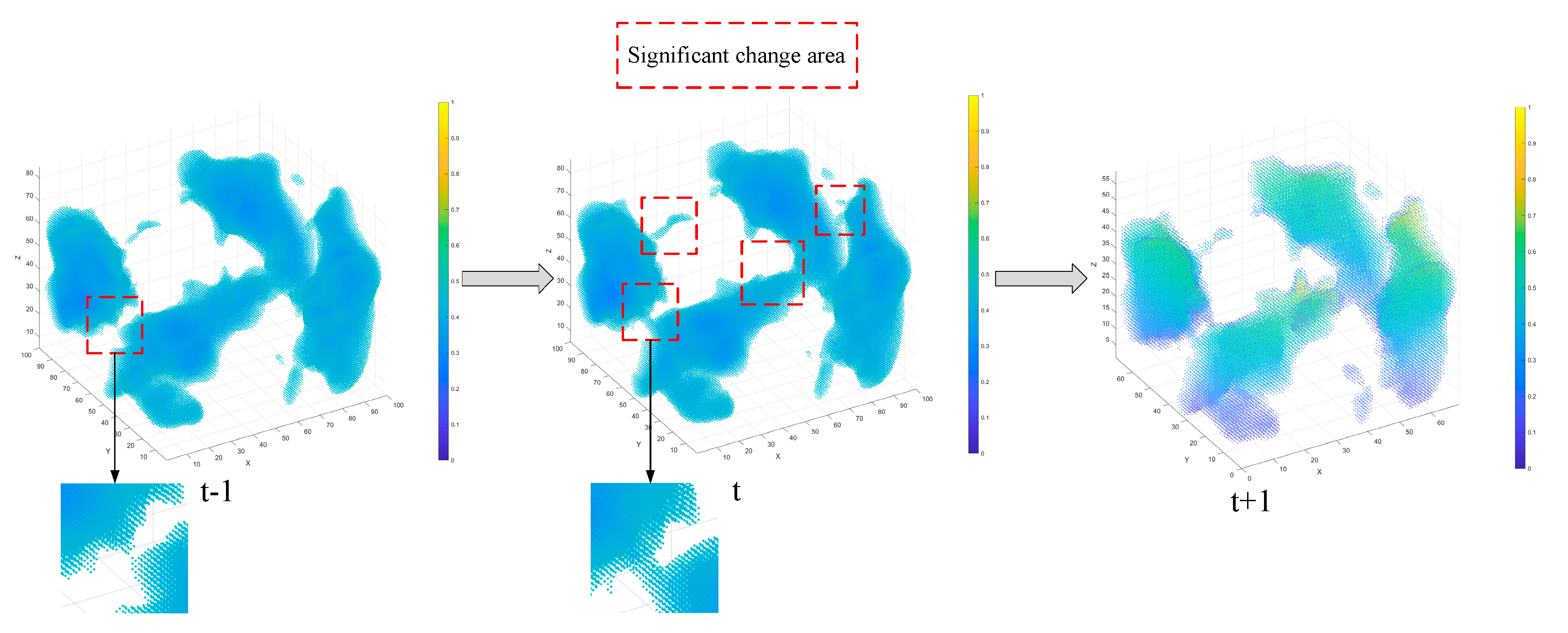
Table 2.
Comparison results.
| Model Name | Accuracy | Recall | F1 Score | PC-Coverage |
| 3D CNN | 0.912 | 0.954 | 0.933 | 0.954 |
| ConvLSTM | 0.903 | 0.978 | 0.939 | 0.978 |
| UNet3D | 0.842 | 0.894 | 0.867 | 0.894 |
| STConvLSTM | 0.926 | 0.975 | 0.950 | 0.975 |
Table 3.
Comparison results.
| STConvLSTM | Accuracy | Recall | F1 Score | PC-Coverage | ||
| Fixed voxel | Only use MSE | Complete model | ||||
| √ | 0.868 | 0.991 | 0.925 | 0.991 | ||
| √ | 0.853 | 0.996 | 0.906 | 0.966 | ||
| √ | 0.924 | 0.970 | 0.947 | 0.970 | ||
Disclaimer/Publisher’s Note: The statements, opinions and data contained in all publications are solely those of the individual author(s) and contributor(s) and not of MDPI and/or the editor(s). MDPI and/or the editor(s) disclaim responsibility for any injury to people or property resulting from any ideas, methods, instructions or products referred to in the content. |
© 2025 by the authors. Licensee MDPI, Basel, Switzerland. This article is an open access article distributed under the terms and conditions of the Creative Commons Attribution (CC BY) license (http://creativecommons.org/licenses/by/4.0/).
Copyright: This open access article is published under a Creative Commons CC BY 4.0 license, which permit the free download, distribution, and reuse, provided that the author and preprint are cited in any reuse.


