

Submitted:
10 November 2025
Posted:
12 November 2025
You are already at the latest version
Abstract
Digital twin applications for water resource recovery facilities require frequent model recalibration to maintain predictive accuracy under dynamic operational conditions. Current calibration methodologies face critical limitations: manual protocols demand extensive expert intervention and iterative parameter adjustments spanning weeks to months, while automated optimization algorithms impose elevated computational burdens that struggle to converge within practical timeframes. This study introduces Expert Systems with Neuro-Evolution of Augmenting Topologies (ES-NEAT), integrating genetic algorithms, artificial neural networks, and transfer learning to preserve and transfer calibration knowledge across recalibration scenarios. Application to the full-scale Eindhoven WRRF over six months, calibrating 33 parameters across multiple temporal scenarios, demonstrated 72.1% and 49.0% Kling-Gupta Efficiency improvement over manual calibration for tank-in-series and compartmental model structures, respectively. Transfer learning reduced subsequent recalibration computational time by 50-70% while maintaining prediction accuracy, transforming initial 10-12 hour optimizations into 3-6 hour recalibrations through knowledge preservation. Performance degradation analysis established 2-month optimal recalibration intervals under observed operational variability. The methodology enables practical digital twin implementation by transforming recalibration from episodic expert-dependent burden into continuous, automated learning processes operating at timescales matching operational decision-making needs.
Keywords:
artificial neural networks
; automatic recalibration
; digital twins
; plant-wide calibration
; transfer learning
1. Introduction
Water Resource Recovery Facilities (WRRFs) are increasingly embracing digital transformation. Unlike traditional simulation models, digital twins maintain continuous, automated data connections with physical assets, enabling real-time performance evaluation, predictive analytics, and operational optimization (Torfs et al., 2022). Recent implementations demonstrate substantial operational benefits: the Eindhoven WRRF in the Netherlands operates with digital twin simulation frequencies every 2 hours and 48-hour forecast horizons, with the combination of advanced data pipeline and process model development making the twin a valuable asset for decision making with long-term reliability (Daneshgar et al., 2024). Digital twin platforms utilizing microservices architecture enable scalable, real-time monitoring and predictive capabilities across multiple treatment facilities (Rodríguez-Alonso et al., 2024). Full-scale implementations in Denmark have documented cost reductions ranging from 9-30% and greenhouse gas emission reductions as high as 35-43% through digital twin-enabled model predictive control (Stentoft et al., 2021).
These gains, however, depend on maintaining model accuracy. Unlike conventional simulation models, digital twins extend these by continuous synchronization with real-time plant data and the physical system they represent (Torfs et al., 2022). This requirement creates an important calibration challenge. Traditional models are calibrated once during commissioning and occasionally validated, whereas operational digital twins require the capability for recalibration to account for changes in process conditions, operations, and sensor performance. These changes can be categorized into several key types: operational disturbances such as fluctuations in industrial discharges, control strategy modifications, and wet-weather flows alter influent composition and loading patterns, requiring updated stoichiometric and kinetic parameters to maintain predictive accuracy (Stentoft et al., 2021). Seasonal temperature variations alter biological kinetics and settling characteristics, with nitrogen removal efficiency dropping from 86.5% to 80.6% when wastewater temperature falls below 15 °C due to shifts in reaction rates and solid-liquid separation behavior, including altered extracellular polymeric substances composition (Xie et al., 2025). Sensor drift further reduces input reliability and reinforces the need for regular recalibration, with drift exceeding 1 mg/L, representing 33% error in typical ammonia measurements, commonly occurring between maintenance intervals (Hansen et al., 2022; Samuelsson et al., 2023).
Maintaining model accuracy is essential not only for process reliability but also for realizing the economic potential of digital twins. Accurate and well-calibrated models enable optimized control strategies that can reduce operating costs by 9-30% depending on control objectives (Stentoft et al., 2021), and improve energy efficiency through more precise process optimization. The challenge intensifies when considering recalibration frequency requirements: sensor cleaning occurs weekly, sensor calibration every two weeks to monthly when drift exceeds 15%, model parameter adjustments seasonally as temperatures shift, and event-driven recalibrations following operational changes (Hansen et al., 2022). Each recalibration episode demands computational resources and expert oversight, creating a burden that scales linearly with plant complexity and operational variability.
The water treatment modeling community has developed two primary approaches to address calibration challenges: structured manual protocols and automated optimization algorithms. Manual calibration protocols, exemplified by BIOMATH (Vanrolleghem et al., 2003), STOWA (Hulsbeek et al., 2002), and WERF (Melcer et al., 2003) methodologies, provide systematic frameworks for parameter adjustment. These protocols leverage expert knowledge to guide stepwise calibration procedures, beginning with hydraulic characterization through tracer studies, progressing through influent characterization using respirometric methods, and culminating in biological process calibration with sensitivity analysis (Sin et al., 2005). The structured, sequential nature of these approaches offers significant advantages: they systematically prevent arbitrary parameter adjustments, avoid local minima through careful parameter subset selection, and integrate process understanding with mathematical optimization.
However, these advantages come at considerable cost. BIOMATH protocols require 3-4 weeks minimum, including one week for data collection, 1-2 weeks for laboratory experiments, and one week for calibration iterations (Vanrolleghem et al., 2003). STOWA implementations span 1-3 weeks with 5-7 days sampling campaigns plus calibration iterations (Hulsbeek et al., 2002). WERF’s tiered approach ranges from days to 8 weeks, depending on calibration depth (Melcer et al., 2003). Beyond time investment, these protocols demand specialized expertise spanning process engineering, activated sludge model structures, statistical evaluation, and laboratory techniques (Zhu et al., 2015). The predominant manual nature of these workflows makes them inherently difficult to automate, limiting their applicability to the recalibration framework demanded by digital twin operations (Sin et al., 2008).
Automated optimization algorithms offer a contrasting approach. Commercial software platforms like GPS-X (Hydromantis, 2017), BioWin (EnviroSim, 2008), and WEST (DHI, 2022) integrate optimization tools based on genetic algorithms, particle swarm optimization, and gradient-based methods. These algorithms systematically search the parameter space to minimize prediction errors, offering a consistent methodology without requiring expert judgment at each decision point. Recent applications demonstrate promising results: optimization of ASM2d model parameters coupled with genetic algorithms achieved up to 75% calibration efficiency compared to manual expert-driven tuning, with reductions in absolute errors for TN and COD to 4.72 and 15.17%, respectively (Yu et al., 2025). Bayesian optimization methods have achieved R2 values exceeding 0.725 for predicting effluent total nitrogen and energy consumption (Ye et al., 2024).
Yet automated algorithms face fundamental limitations. Convergence to local optima remains persistent for overparameterized activated sludge models containing 30-40+ parameters with complex interactions. Parameter identifiability issues, where highly correlated parameters (such as growth rates for ammonia-oxidizing and nitrite-oxidizing bacteria with correlation coefficients of 0.99) cannot be reliably estimated simultaneously, further complicate optimization (Petersen et al., 2003; Zhu et al., 2015). Computational costs remain substantial; genetic algorithms typically require 2500-20,000 function evaluations, while particle swarm optimization demands 2000-25,000 iterations. For dynamic simulations spanning over a year, each function evaluation consumes minutes to hours, extending total calibration time to days, even with parallel processing. Most critically, particle swarm optimization faces documented restrictions, including premature convergence and getting stuck in locally optimal points (Peirovi Minaee et al., 2019).
Most critically for digital twin applications, current automated approaches suffer from a knowledge loss problem: they restart calibration from scratch for each new scenario, discarding the structural information about which parameter combinations work well together and how to navigate the optimization landscape. Rather than preserving insights about parameter relationships and optimization pathways gained during previous calibrations, algorithms reinitialize to default values or random starting points. This means computational burden scales linearly with recalibration frequency; facilities requiring monthly parameter updates face 12 times the annual calibration effort compared to those updating only once yearly, with proportional increases in expert time and computational resources (Duarte et al., 2023). This knowledge loss problem creates a fundamental barrier to practical digital twin implementation, as the reality of frequent manual recalibration or computationally expensive automated recalibration undermines their viability.
Transfer learning offers a promising yet unexplored solution to this recalibration knowledge loss problem. The fundamental principle, leveraging knowledge gained from solving one problem to accelerate learning in related problems, has demonstrated remarkable success across diverse engineering domains. In nuclear reactor transient prediction, physics-informed neural networks with transfer learning achieved 10-100 fold computational speedup while maintaining mean errors below 1% (Prantikos et al., 2023). High-frequency multi-scale problems saw training time reductions from 75,000 iterations to fewer than 2,000, representing a 37.5× speedup (Mustajab et al., 2024). Finite element model calibration achieved at least 2× faster performance while maintaining inversion errors consistently below 2% (Zhou & Mei, 2023).
Within water and wastewater applications specifically, transfer learning has enabled breakthrough capabilities. Viral particle prediction across multiple treatment plants achieved mean R2 values of 0.96 through lifelong learning frameworks that transferred knowledge between facilities with different treatment processes (Chen et al., 2025). Cross-basin water quality prediction attained mean Nash-Sutcliffe efficiency of 0.80 across 149 monitoring sites by pre-training on six major river basins and fine-tuning for local conditions (Zheng et al., 2025). Dissolved oxygen prediction in industrial wastewater treatment improved by 27-59% when transfer learning combined knowledge from simulation models with limited plant data (Koksal & Aydin, 2024). Control system design for wastewater plants successfully transferred learned controller parameters between different process loops, reducing design time from hours or days per artificial neural network (Pisa et al., 2021).
Despite these successes in control design, soft sensor development, and water quality prediction, transfer learning has never been applied to mechanistic model calibration for water resource recovery facilities. The transition to digital twins demands the ability to “dynamically update or adjust the models based on relevant data to maintain an accurate description of the real entity as it evolves over time,” recognized as “a challenging aspect to include in a DT” (Torfs et al., 2022), but no documented approaches preserve or transfer calibration knowledge between recalibration instances. Recent comprehensive reviews of activated sludge modeling explicitly identify calibration as a persistent barrier; “a time-consuming step that hinders the broader application of these models” requiring “a considerable level of expert knowledge of the process”, yet propose no transfer learning solutions (Ruela et al., 2023; Rashid et al., 2024). This gap is particularly striking given that the same research community successfully applies transfer learning to control problems that exhibit similar challenges: changing operational conditions, sensor drift, and seasonal variations.
This study addresses the recalibration knowledge loss problem through a novel methodology that integrates genetic algorithms, artificial neural networks, and transfer learning for automatic water resource recovery facility model calibration. The Expert Systems with Neuro-Evolution of Augmenting Topologies approach constructs neural network architectures specifically tailored for calibration parameter estimation, then preserves and transfers learned knowledge across recalibration episodes. Rather than discarding optimization insights, the methodology initializes each recalibration using evolved neural networks that encode previous calibration knowledge, enabling rapid adaptation to changed conditions while maintaining prediction accuracy.
The research objectives are: first, to validate the methodology on a full-scale facility operating under realistic dynamic conditions; second, to quantify computational savings achieved through transfer learning compared to standard recalibration from scratch; and third, to establish optimal recalibration frequency by analyzing the trade-off between computational cost and prediction accuracy degradation. The approach is applied to the digital twin of the Eindhoven water resource recovery facility (Daneshgar et al., 2024) using six months of operational data, calibrating 33 parameters, including kinetic rates, stoichiometric coefficients, and influent composition fractions across multiple operational scenarios. By preserving calibration knowledge rather than discarding it, this methodology aims to transform recalibration from a periodic burden into a continuous learning process that enables truly adaptive digital twins.
2. Materials and Methods
2.1. Case Study: Eindhoven Water Resource Recovery Facility
2.1.1. Eindhoven WRRF: Layout and Model Structure
The Eindhoven WRRF receives wastewater from three major sewer systems, accounting for about 750,000 population equivalents, making it the third largest facility in the Netherlands. The main treatment processes used at the Eindhoven WRRF include preliminary treatment, primary settling, activated sludge treatment, and secondary treatment, which is designed with a modified UCT configuration.
A plant-wide model for the Eindhoven WRRF has been incrementally developed over the past decade (Cierkens et al., 2012; Amerlinck 2015; De Mulder et al., 2018; De Mulder, 2019). Since 2023 the plant-wide model has been implemented and is running as a real-time operational digital twin (Daneshgar et al., 2024). The model’s layout is presented in Figure 1 and is further described in the work of Daneshgar et al. (2024).
The Eindhoven WRRF model employs the Activated Sludge Model no. 2d (ASM2d) (Henze et al., 2006) to describe chemical and biological phosphorus removal. The primary settling tank (PST) was modeled using a modified Tay model (Tay, 1982) with separate removal efficiencies for COD and TSS, while the secondary settling tank (SST) was represented by the Bürger–Diehl model (Bürger et al., 2011) employing a double-exponential settling function. Initially, the tank-in-series (TIS) approach was used to represent mixing behaviour in both aerobic and anoxic zones; further works improved the model with respect to nonideal mixing and prompted the development of a compartmental model (CM) to better capture local heterogeneities in the aeration zone (Rehman 2016, De Mulder 2019).
The model includes several controllers: a linear controller for anaerobic internal recycle (Rec_A) based on influent flow rate, a PI-controller for internal nitrate recycle (Rec_B) based on NO3− measurements in the anoxic zone, a P-controller for regulating sludge waste flow based on the mixed liquor suspended solids set point at the end of the aeration zone, and an aeration controller based on NH4+ levels in the aerobic zone. Additional details on the model can be found in Daneshgar et al. (2024), De Mulder et al. (2018), and Cierkens et al. (2012).
2.1.2. Calibration Dataset and Parameter Specification
The selection of calibration parameters was based on a systematic multi-criteria approach integrating sensitivity analysis, expert knowledge, and calibration objectives. Parameter identification followed the framework established by Benedetti et al. (2008), who performed global sensitivity analysis on activated sludge models to identify the most influential parameters affecting effluent quality predictions. Given the calibration targets (specified in Section 2.3.3), parameters directly governing nitrification, denitrification, and biomass production kinetics were prioritized. Phosphorus-related parameters were excluded from calibration since the plant employs chemical phosphorus removal as a supplementary mechanism when the biological removal capacity is insufficient. Initial parameter ranges were established from literature values provided in the ASM2d reference (Henze et al., 2006), expanded by ±20-50% to account for site-specific variations, and refined through expert judgment from plant operators and stakeholders as described by Daneshgar et al. (2024). The final parameter set (Table 1) comprised 33 kinetic, stoichiometric, and settling parameters as well as influent fractions, with search ranges constrained to physically meaningful values.
Online sensor data for NH4+, NO3−, and TSS at the end of the aeration zone (before the secondary settling tank) are available, as well as NO3− measurements in the anoxic zone, for six months in 2013 at 15-minute measurement intervals. Similarly, online data for influent flow rate, total COD (CODt), soluble COD (CODs), TSS, NH4+, and phosphate (PO43−) in the influent are available for six months at 15-minute measurement intervals. All data underwent extensive cleaning and reconciliation processes to remove outliers and fill gaps using various interpolation and mass balance techniques. This six-month period was selected because it represents a dataset that has undergone rigorous data quality control and was previously used for comprehensive manual calibration efforts (De Mulder et al., 2018), providing a validated foundation for methodological comparisons. Three temporal scenarios (July, September, and November 2013) were selected from this six-month dataset for recalibration analysis; detailed descriptions of scenario structure and selection rationale are provided in Section 2.4.1. Figure 2 presents the variability and dynamics of influent flow rate, total suspended solids (TSS), chemical oxygen demand (COD), and ammonium (NH4+) for each scenario.
The WRRF model was previously calibrated by De Mulder et al. (2018) using data from the November 2013 period, establishing the original calibration parameter set that serves as the baseline for this study (detailed methodology in Section 2.3.1). Both the automatic calibration methods and the original calibration were initialized from default literature values provided in the ASM2d reference (Henze et al., 2006).
2.2. Novel Calibration Methodology: ES-NEAT
The ES-NEAT automatic calibration methodology (Gomez et al., 2025) integrates Expert Systems (ES) (Kaisler, 1986) with Neuro-Evolution of Augmenting Topologies (NEAT) (Stanley & Miikkulainen, 2002) to construct neural networks tailored for calibrating WRRF models. The methodology enables efficient global calibration of highly parameterized systems while incorporating a transfer learning approach for accelerated recalibration processes. The conceptual scheme is shown in Figure 3. Complete hyperparameter specifications and implementation details are provided in the GitHub Code Repository Section.
The core of the ES-NEAT method is a neural network that outputs values for the 33 calibration parameters previously defined in Table 1. The neural network receives 10 input variables representing averaged measurements from the modeled plant: influent CODs, influent CODt, influent NH4+, influent PO43−, influent TSS, influent flow rate, anoxic zone effluent NO3−, end of aeration zone effluent NH4+, end of aeration zone effluent NO3−, and end of aeration zone effluent TSS. All input variables were normalized to [0,1] using min-max scaling.
2.2.1. NEAT: Neuro-Evolution of Augmenting Topologies
NEAT optimizes the neural network topology so that the neural network outputs optimally calibrated parameters. Since traditional backpropagation is not feasible due to the absence of known target parameter values for loss calculation, NEAT evolves both topology and connection weights using genetic algorithms. The methodology was implemented using the NEAT-Python library version 0.92 (Stanley & Miikkulainen, 2002).
Initial generations consist of 100 randomly generated networks with minimal topology, which evolve through mutation, crossover, and speciation. The optimization process focused on evolving the network structure, including the number of layers, nodes, and connectivity between neurons. In addition to topology, NEAT optimized the connection weights and biases, determining the strength of relationships between neurons and activation thresholds. The node activation function was set to sigmoid for all layers, including the output layer. Additional hyperparameters, including node and connection addition/removal rates, followed the default configurations of the NEAT-Python library. Each network is evaluated using the objective function described in Section 2.3.1. Superior topologies propagate to subsequent generations with an elitism rate of 10%, meaning 90 new neural networks are created in each generation, while the best 10 are retained from the previous generation.
Originally developed for robotic control, NEAT performs well in high-dimensional search spaces and is suited for calibration problems where gradient-based methods are ineffective (Mnih et al., 2013). Its ability to navigate complex parameter landscapes without relying on fixed topologies allows it to align model outputs with empirical data while mitigating the risk of getting stuck at local optima. The methodology was configured with a population size of 100 individuals (i.e., 100 distinct neural networks evolving simultaneously in each generation), a maximum of 100 generations, and a fitness threshold based on an objective value of 0.75.
2.2.2. ES: Expert Systems
While NEAT governs the network structure and evolution, ES defines parameter constraints by encoding domain knowledge, including value ranges, probability distributions, and discretization steps. These constraints, derived from literature (Henze et al., 2006) and expertise from plant operators, improve convergence speed and ensure physical plausibility of calibrated parameters.
The ES comprises a knowledge base and inference engine that generates parameter ranges based on rules and heuristics. In this study, triangular probability distributions were implemented for all parameters within the ranges presented in Table 1, concentrating sampling around mean parameter values. All WRRF parameters were calibrated simultaneously without grouping.
Expert systems play a crucial role by incorporating domain-specific knowledge and logical reasoning to generate constraints that guide the optimization process. Without expert-driven guidance, the convergence of NEAT would be significantly prolonged, as the algorithm would need to explore a much larger search space. Expert systems direct the search toward promising regions, accelerating convergence and reducing computational effort. Furthermore, they ensure parameter values remain within realistic and physically meaningful ranges, preventing unrealistic configurations and reducing the likelihood of the optimization becoming trapped in local optima. The final output of the ES-NEAT method is a neural network embedding parameter behavior, interactions, and feasible ranges within its structure.
2.2.3. Transfer Learning for Recalibration
A key innovation of this methodology is the implementation of transfer learning to accelerate the recalibration process when operational conditions change. Using NEAT’s checkpoint save/load functionality, the final population state from a completed calibration, including all 100 evolved neural networks with their topologies, connection weights, and biases, are saved and subsequently reloaded as the initial state for the next recalibration round. This approach leverages the optimized network topology discovered during initial calibration rather than restarting evolution from minimal network structures. Upon reloading, connection weights and biases are preserved as-is from the previous calibration, and the evolutionary process resumes with the capability for further structural modifications. By inheriting the calibrated topology and population from previous optimizations, the recalibration process converges substantially faster than calibration from minimal topologies, as the neural networks start from a configuration already adapted to the system’s hydraulic and biological behavior. This transfer learning approach enables the accumulated calibration knowledge to be applied efficiently to future scenarios, promoting generalization, reducing overfitting, and improving computational efficiency in subsequent applications.
2.3. Benchmark Comparison Cases Against the Proposed Method
To evaluate the effectiveness of the proposed ES-NEAT approach, two baseline methods were included for comparison: the original calibration performed by De Mulder et al. (2018) and Particle Swarm Optimization (PSO).
2.3.1. Baseline Manual Calibration
The original calibration was performed by De Mulder et al. (2018) using systematic manual protocols that integrated sensitivity analysis, expert knowledge, and iterative parameter adjustment. This calibration established the baseline parameter set for the Eindhoven WRRF model using data from the November 2013 period. The process focused on optimizing influent fractions, kinetic parameters, settling parameters, and aeration model parameters, with particular emphasis on fine-tuning the nitrogen content of inert soluble COD (Si) and the ammonium half-saturation coefficient for autotrophs (K_NH_AUT). The calibration targeted NH4+ and NO3− concentrations at the end of the aeration zone, with parameter adjustments designed to maintain predictive accuracy across the six-month study period. The original calibration required approximately one month of expert effort, providing a benchmark for time demands associated with manual approaches.
2.3.2. Particle Swarm Optimization (PSO) Benchmark
Particle Swarm Optimization was included as an additional automated benchmark to demonstrate that the improvements achieved by transfer learning stem not merely from automation, but from the specific methodology of leveraging knowledge from previously calibrated scenarios. PSO was selected as the automated optimization benchmark based on its established use in WWTP calibration literature and its recognition as a standard metaheuristic approach for parameter estimation in water quality modeling (Protoulis et al., 2023; Peirovi Minaee et al., 2019). Furthermore, PSO exhibits superior robustness to local optima compared to gradient-based optimization methods, making it particularly appropriate for the non-convex characteristic of parameter spaces in WWTP models.
The algorithm was implemented using the PySwarms Python library version 1.3.0 (Miranda, 2018) with default parameters for cognitive coefficient (c1), social coefficient (c2), and inertia weight (w), following the Local Best PSO topology. PSO was configured with the same population size (100 particles), maximum iterations (100), convergence criteria (KGE threshold of 0.75), and objective function as ES-NEAT to ensure fair comparison. The PSO method was included exclusively in the July calibration scenario to establish a performance baseline for comparison with ES-NEAT within automatic calibration frameworks.
2.3.3. Objective Function and Performance Metrics
The primary objective function for ES-NEAT and PSO calibration is the Kling-Gupta Efficiency (KGE) metric (Gupta et al., 2009), which evaluates model performance by decomposing prediction quality into three components: correlation, bias, and variability. KGE is calculated as:
where r is the Pearson correlation coefficient between observed and simulated values, α is the ratio of standard deviations (simulated/observed), and β is the ratio of means (simulated/observed). KGE values range from -∞ to 1, with 1 indicating perfect agreement.
For each of the four target variables (anoxic zone NO3−, end of aeration zone NH4+, end of aeration zone NO3−, and end of aeration zone TSS), the KGE was calculated independently between observed and simulated time series. The final fitness score was computed as the arithmetic mean of KGE values across all monitored target variables, ensuring equal weighting and avoiding range mismatch issues in the multi-objective optimization. In addition to KGE, two complementary metrics were implemented: RMSE and R2, which are described in Appendix H.
Convergence Criteria. Two convergence criteria were implemented to terminate the optimization process:
- KGE improvement threshold: The algorithm terminated when the final fitness score (i.e., average KGE) reached or exceeded 0.75, indicating satisfactory model performance.
- Maximum iterations: A maximum iteration limit of 100 was imposed to prevent excessive computational time, with the algorithm terminating after reaching this threshold regardless of KGE performance.
The optimization concluded when either criterion was satisfied, and the best parameter set achieving the highest fitness score was retained as the calibrated model configuration.
Transfer Learning Effectiveness. To evaluate the efficiency of different calibration approaches, two key performance indicators were tracked:
- Final number of iterations: The total number of optimization iterations required to reach convergence (either by satisfying the KGE threshold or reaching maximum iterations).
- Final accuracy: The best fitness score (average KGE across all effluent parameters) achieved at termination.
2.4. Experimental Design Framework for Model Recalibration
Table 2 presents the complete experimental design structure, detailing the hierarchical organization of variables evaluated in this study.
2.4.1. Main Calibration Scenarios
Three temporal scenarios (July, September, and November 2013) were selected to evaluate model recalibration performance across varying seasonal and operational conditions. Each scenario comprises a 24-day period: two weeks (days 1-14) for calibration and one week (days 15-21) for validation, followed by an additional three-day buffer (days 22-24) to assess short-term parameter stability. These scenarios were spaced approximately one month apart to capture intermediate-term variations in influent characteristics and biological system responses.
Two model structures were evaluated for each scenario: the Tank-in-Series (TIS) model, which represents the original modeling approach with simplified hydraulic assumptions, and the Compartmental Model (CM), which incorporates refined spatial resolution and mixing patterns in the aeration zone. This dual-structure evaluation enables assessment of methodology robustness across different levels of model complexity.
Three calibration methods were compared in the July scenario: ES-NEAT, PSO, and the original calibration established by De Mulder et al. (2018). For September and November scenarios, only ES-NEAT and the original calibration were evaluated, as PSO served exclusively as a benchmark for demonstrating the advantages of transfer learning over conventional automated optimization approaches. ES-NEAT employed transfer learning for September and November recalibrations, reloading the final population state from the previous temporal scenario as the initial condition rather than starting from minimal network topologies.
2.4.2. Recalibration Frequency Analysis
To evaluate the impact of recalibration frequency on model performance, three distinct frequency scenarios were analyzed: recalibration at 4-month intervals (July to November), 2-month intervals (July to September, September to November), and 3-week intervals (continuous weekly updates within each monthly scenario). Both ES-NEAT and the original calibration methods were evaluated across all frequency levels.
Model performance was assessed during a common evaluation period from October 15 to November 10, divided into two distinct phases: two weeks immediately preceding the November recalibration (October 15-28) and two weeks following the recalibration (October 29–November 10). This temporal structure enabled direct comparison of performance degradation over time and the effectiveness of recalibration in restoring model predictive accuracy.
2.4.3. Statistical Validation
Statistical analysis was performed on three performance metrics (KGE, R2, and RMSE) for each of the four target variables previously defined. The experimental design yielded a hierarchical data structure as detailed in Table 2. Three independent simulation replicates were conducted for each method-scenario-model combination to ensure statistical robustness, where each replicate represents a complete execution of the calibration workflow with identical initialization conditions but potentially different stochastic elements in the optimization algorithms.
Each 24-day calibration scenario was subdivided into three consecutive 8-day periods (days 1-8, 9-16, and 17-24) for statistical analysis purposes. This temporal subdivision was essential for capturing within-scenario temporal variability and assessing parameter stability throughout the calibration period, as model performance may deteriorate or stabilize over time following parameter adjustment. Statistical analyses were performed separately on data from each 8-day period to evaluate the temporal consistency of method performance.
Three complementary statistical approaches were implemented to comprehensively evaluate method performance, each providing distinct analytical perspectives. Paired t-tests enabled direct pairwise method comparisons while controlling for within-group variability. Linear mixed-effects models assessed population-level method effects and interactions while accounting for hierarchical data structure. Confidence intervals quantified estimation precision and facilitated interpretation of practical significance. Together, these approaches provided robust statistical inference across multiple levels of analysis.
Paired t-tests (α = 0.05) were conducted to compare calibration methods within matched experimental conditions. Pairing was implemented to control for confounding variables inherent in the hierarchical structure, specifically matching observations by target variable, temporal period, scenario, and model type. This pairing strategy eliminated between-group variability attributable to these factors, thereby increasing statistical power to detect method differences. Three pairwise comparisons were evaluated: ES-NEAT versus original calibration, ES-NEAT versus PSO, and PSO versus original calibration. The assumption of normality for paired differences was assessed using Shapiro-Wilk tests before inference. Cohen’s d was used to measure effect size as the standardized mean difference between groups, with values of 0.2, 0.5, and 0.8 indicating small, medium, and large practical effects, respectively. This metric distinguishes statistically significant results from practically meaningful improvements. The False Discovery Rate (FDR) correction, via the Benjamini-Hochberg procedure, controls the expected proportion of false positives when performing multiple statistical tests. Applied across 18 scenario-metric combinations, this correction maintains statistical validity while accounting for repeated hypothesis testing.
Linear mixed-effects models were fitted to assess main effects and interactions while accounting for the nested and repeated-measures structure of the data. Mixed models were selected for their capacity to handle hierarchical data structures, unbalanced designs resulting from the inclusion of PSO only in July, and potential missing data, thereby providing advantages over traditional repeated measures ANOVA. The fixed effects structure included Method, Scenario, Variable, and their two-way interactions (Method × Scenario and Method × Variable), capturing systematic differences between calibration methods at the population level. Random effects were specified with Model nested within Scenario and Temporal Period (referring to the three 8-day subdivisions within each scenario), accounting for variability across different experimental contexts and temporal replicates. Under this framework, fixed effects quantified the average performance differences between methods, while random effects captured the extent to which these differences varied across model structures, scenarios, and temporal periods.
95% confidence intervals were calculated for all performance metrics to complement hypothesis testing by providing effect size interpretation beyond binary significance decisions. Confidence intervals were constructed using the t-distribution with appropriate degrees of freedom, accounting for sample size and variance structure within each comparison. This approach enabled assessment of estimation precision and facilitated evaluation of whether observed differences were both statistically significant and practically meaningful for wastewater treatment plant calibration applications.
Results from all three statistical approaches were synthesized to ensure robust conclusions. Convergent evidence across paired t-tests, mixed-effects models, and confidence interval analyses was required to establish definitive method superiority, while discrepancies between approaches informed interpretation of context-dependent performance patterns.
2.5. Implementation Computational Setup
The WEST simulation tool (DHI, Denmark, version 2023) and Python (version 3.12.4) were utilized for the model calibration. WEST provided a robust modeling platform for simulating dynamic wastewater treatment processes and a user-friendly interface, while Python enabled automation of workflows and optimization through its data analysis libraries, ensuring efficient and reliable calibration. The experiments were conducted on a system with an 11th Gen Intel Core i5-1145G7 processor (2.60 GHz base, 4.40 GHz turbo), 16 GB RAM, and Windows 10 (64-bit). The NEAT method was implemented with multiprocessing to enhance simulation efficiency, enabling the simultaneous execution of eight computational simulations. These simulations, which evaluated WRRF models with varying parameters determined by the ES-NEAT methodology, were run concurrently to reduce overall computational time significantly. By leveraging parallelization, multiple scenarios were processed at once, improving the speed of the simulations and drastically cutting down the time required for completion. All methods use the same parallelization pipeline for fair comparison. Computational time for all calibration methods was recorded throughout the optimization process for subsequent efficiency analysis.
3. Results and Discussion
3.1. Performance Comparison of Calibration Methods
ES-NEAT consistently achieved superior performance across all scenarios and model types. Aggregated across variables and periods, the CM model performance ranked as ES-NEAT (mean KGE: -0.197) > PSO (-0.262) > Manual (-0.386), while TIS model showed ES-NEAT (-0.303) substantially outperforming Manual (-1.088), representing 49.0% and 72.1% improvements for CM and TIS, respectively (Figure 4, Table 3). Statistical validation confirmed ES-NEAT significantly outperformed Manual in 7 of 18 scenario-metric combinations (p < 0.05), with 6 additional practically meaningful improvements (see Appendix D for complete statistical analyses and Appendix A for the full time-series plots).
The neural network evolution process explored parameter interactions simultaneously, enabling globally superior parameter combinations compared to sequential manual adjustments. The expert system constrained searches using domain knowledge through triangular probability distributions, accelerating convergence while maintaining physical realism. Population-based evolutionary strategy maintained diversity through speciation, preventing premature convergence common in gradient-based methods.
Validation performance revealed critical methodological differences across the three sequential scenarios. ES-NEAT maintained relatively stable validation performance, while Manual calibration showed progressive degradation over time. This divergence demonstrates that automated optimization with knowledge preservation capabilities maintains accumulated insights, whereas manual approaches lose learning between recalibration events. Computational efficiency gains were substantial, with automated methods achieving calibration within hours compared to manual approaches requiring weeks. Detailed time savings through transfer learning are presented in Section 3.2.
Performance varied systematically across monitored variables. Aerobic Tank NH4 and Aerobic Tank NO3 showed improvements under automated calibration, while Anoxic Tank NO3 remained challenging across all methods, indicating fundamental model structural inadequacy rather than calibration failure (detailed analysis in Section 3.5). Overall performance patterns validated across both CM and TIS model structures, confirming benefits originate from calibration methodology rather than model artifacts. The consistent method ranking across hydraulic representations demonstrates robust advantages. Detailed variable analyses and TIS model results are in Appendix B and Appendix C.
3.2. Transfer Learning Effectiveness
Transfer learning provided substantial computational savings while maintaining accuracy. Manual calibration required approximately 720 hours per event, including iterative parameter adjustments and expert judgment. Automated methods without transfer learning achieved initial calibration within 12 hours (CM) and 10 hours (TIS). Following July baseline, September recalibration with transfer learning achieved 67% time reduction for CM (4 hours) and 70% for TIS (3 hours). November recalibration, despite 4-month separation, still achieved 50% savings (CM: 6 hours; TIS: 5 hours). Performance maintained or exceeded July levels: September CM achieved calibration KGE of -0.069 versus July 0.017; TIS produced 0.065 versus July -0.125. Cumulative savings across three calibrations totaled 39% (CM) and 40% (TIS) compared to repeated full optimizations (see Appendix D for convergence patterns). Transfer effectiveness decreased with temporal separation but remained beneficial across extended periods. July-to-September (2 months) demonstrated great benefits, while direct July-to-November (4 months) showed reduced but substantial advantages. This temporal pattern is explored in detail in Section 3.4.
Scenario similarity critically influenced transfer success. July-September exhibited similar loading patterns (mean influent COD: 715 vs. 616 mg/L; NH4+: 36.3 vs. 39.9 mg/L), enabling direct topology transfer with minimal adjustment. September-November showed greater divergence (November mean COD: 548 mg/L; NH4+: 39.7 mg/L), necessitating more extensive re-exploration and extending calibration from 3-4 to 5-6 hours. Transfer learning performs best when consecutive scenarios share similar operational characteristics, with prior calibrations capturing relevant dynamics applicable under comparable conditions.
Parameter stability classification explained transfer effectiveness mechanistically. Stable parameters (CV < 10%): stoichiometric coefficients and nitrogen fractions showed minimal drift, requiring no recalibration. Transfer learning provided minimal benefit here as values remained constant. Variable parameters (CV > 20%): kinetic rates and settler characteristics required substantial adjustment but benefited from initializing at previously successful values rather than literature defaults. Moderate parameters (10% < CV < 20%): growth yields and half-saturation coefficients exhibited strongest transfer benefits, requiring scenario-specific tuning within consistent ranges. Evolved networks encoded approximate values and parameter interactions, enabling localized refinement rather than global search, achieving the time reductions documented above. Detailed parameter classifications are presented in Section 3.3.
Statistical validation confirmed these benefits. Mixed-effects models showed significant ES-NEAT improvements for TIS, with Method × Variable interactions revealing differential effectiveness across output variables. Correlation analysis quantified progressive improvements: TIS overall R2 showed significant positive correlation with recalibration sequence, with multiple variables demonstrating significant gains. These analyses support the performance advantages documented in Section 3.1.
Comparison with PSO highlighted transfer learning’s unique contribution. Both ES-NEAT and PSO achieved comparable July baseline performance, confirming competitive standing among metaheuristics for single-event optimization. However, PSO required full 12-hour recalibrations in September for both models, whereas ES-NEAT leveraged transfer to complete in 3-4 hours; a threefold efficiency gain. This illustrates that ES-NEAT’s advantage lies in knowledge preservation absent from standard metaheuristics restarting from random initializations. Cumulative efficiency across three calibrations demonstrates the compounding benefit: ES-NEAT totaled 22h (CM) and 18h (TIS) versus hypothetical 36h and 30h for repeated PSO optimizations without knowledge transfer, representing approximately 40% cumulative savings.
Transfer learning cannot overcome structural deficiencies, however. Variables with adequate model representations showed progressive improvement, while structurally limited variables showed no benefits despite repeated attempts. This diagnostic capability, revealing when parameter optimization reaches structural performance ceilings, is examined in detail in Section 3.5.
3.3. Parameter Stability and Recalibration Needs
Across three scenarios, 33 calibration parameters were classified into three stability categories based on the coefficient of variation. For CM, 10 parameters achieved Stable classification (CV < 10%): nitrogen content fractions (i_N_BM, i_N_X_I, i_N_X_S), TSS fractions, and half-saturation coefficients (K_NH_AUT, K_fe). Six showed Moderate variability (10-20% CV): Y_AUT, K_NO, SST.v0, Y_H, and influent fractions. Seventeen were classified as Variable (CV > 20%): decay rates (b_H, b_AUT), maximum growth rates (mu_AUT), hydrolysis coefficients (k_h), and settler parameters. TIS showed similar distributions with consistent patterns across model structures (complete tables in Appendix F).
Functional group analysis revealed systematic hierarchies. Stoichiometric coefficients are predominantly classified as Stable (83% of members), reflecting biochemical constraints less sensitive to environmental fluctuations. Half-saturation coefficients showed bimodal distribution: substrate affinity parameters (K_NH, K_NO, K_O) achieved Moderate-to-Variable classification, while less sensitive parameters remained Stable. Kinetic parameters are universally classified as Moderate-to-Variable, requiring frequent recalibration for seasonal temperature effects and microbial shifts. Settler parameters exhibited the highest variability, reflecting operational control adjustments and unmeasured dynamics.
These patterns inform dimensionality reduction strategies: fixing 10 Stable parameters at optimized values could reduce optimization space from 33 to 23 dimensions (30% reduction), accelerating future convergence while maintaining accuracy. Variable parameters demand frequent recalibration to maintain accuracy, while Moderate parameters serve as candidates for conditional fixation when consecutive scenarios exhibit similar characteristics.
As explained in Section 3.2, parameter stability classifications explain differential transfer learning effectiveness. Moderately variable parameters showed the strongest benefits from knowledge preservation, drifting systematically rather than randomly. Highly Variable parameters required extensive re-exploration but benefited from avoiding unproductive regions encountered in prior calibrations. Stable parameters contributed by remaining fixed once optimal values were identified. This understanding suggests targeted optimization: allocate computational resources proportional to parameter variability, focusing on Variable parameters while maintaining Stable parameters at established values. The parameter behavior patterns documented here, combined with the transfer learning mechanisms described previously, provide a framework for optimizing future recalibration strategies across different operational conditions.
3.4. Impact of Recalibration Frequency
Recalibration frequency analysis compared 4-month, 2-month, and 3-week intervals during October 30–November 29 evaluation period. Progressive degradation with longer intervals followed exponential patterns. The 4-month scenario (last calibration July) showed substantial pre-recalibration degradation: ES-NEAT mean KGE of -0.653 (R2: 0.017), representing 95.8% degradation from July’s optimized performance. The 2-month scenario (last calibration September) exhibited moderate degradation: pre-recalibration KGE of -0.599 (R2: 0.006), representing 86.9% decline. The 3-week scenario demonstrated minimal degradation: pre-recalibration KGE of -0.245 (R2: 0.031), only 59.8% decline. These rates quantify temporal limits of calibration validity under Eindhoven operational variability (complete metrics and plots in Appendix G). To illustrate this process, the evolution of Aerobic Tank TSS is shown in Figure 5.
All frequencies demonstrated clear performance recovery following November recalibration, with more frequent recalibration schedules maintaining models closer to optimal performance throughout the evaluation period. ES-NEAT recovered more effectively than Manual across all scenarios, with automated approaches consistently restoring accuracy more reliably.
Empirical thresholds establish optimal scheduling. Performance remained above 70% of calibrated accuracy when intervals stayed below 1.5 months, representing maximum efficiency with minimal parameter adjustment. Between 1.5-2.5 months, performance declined to 50-70%, indicating that more extensive re-exploration becomes necessary. Beyond 2.5 months, performance dropped below 50%, though successful recalibration remains feasible at extended separations as demonstrated in Section 3.2.
Cost-benefit analysis revealed frequency-dependent tradeoffs. The 4-month frequency required two recalibrations, but experienced extended suboptimal performance. The 2-month period necessitated three recalibrations (22% increased computational cost), achieving improved interim performance. The 3-week period implied six recalibrations (167% increased cost) but maintained consistently high performance. Transitioning from 4-month to 2-month improved mean pre-recalibration KGE by 9.1% for 22% increase in cost (0.41 KGE improvement per computational hour). Further transitioning to 3-week improved KGE by 59.1% for 118% increased cost (0.50 KGE/hour). These calculations suggest 2-month intervals optimize accuracy-efficiency tradeoffs for Eindhoven under observed variability, balancing the time savings enabled by transfer learning with continuous accuracy maintenance needs.
3.5. Model Performance Across Variables
Calibration success in aerobic tanks revealed a clear performance hierarchy: NH4 achieved highest accuracy, TSS demonstrated moderate consistency, and NO3 showed variable but substantial improvements under automated optimization. Aerobic Tank NH4 performed excellently across all methods and scenarios, with November validation demonstrating the strongest calibration-method differentiation (CM: ES-NEAT -0.328 vs. Manual -1.051, representing 68.8% improvement; TIS: ES-NEAT 0.332 vs. Manual -0.062). Aerobic Tank TSS maintained stable moderate performance with minimal method-dependent variation across all temporal scenarios (November CM: ES-NEAT 0.253 vs. Manual 0.282), indicating successful solids transport representation. Aerobic Tank NO3 exhibited strong ES-NEAT advantages, particularly in CM configurations, with July showing the largest method difference (calibration KGE: ES-NEAT 0.016 vs. Manual -0.982, representing 98.4% improvement).
These aerobic tank variables demonstrated consistent high accuracy, indicating biological nitrogen removal and solids separation processes are adequately represented by current model structures. Successful calibration across temporal scenarios confirms that underlying process formulations capture essential system behaviors. The moderate performance variability across calibration methods, with automated optimization providing incremental improvements over reasonable manual baseline performance, indicates that model structural adequacy enables effective parameter identification. When physical and biochemical process representations appropriately capture system dynamics, even basic manual calibration achieves acceptable approximations, while sophisticated automated optimization refines these to extract additional accuracy gains.
Anoxic Tank NO3 consistently produced the poorest performance across all variables, methods, and temporal scenarios. Representative results demonstrate persistent failure: July (CM Manual -0.470, ES-NEAT -0.368; TIS Manual -1.923, ES-NEAT -0.403), September (CM Manual -0.080, ES-NEAT -0.672; TIS Manual -1.548, ES-NEAT -1.091), and November (CM Manual -1.563, ES-NEAT -0.520; TIS Manual -5.624, ES-NEAT -2.402). Despite ES-NEAT achieving relative improvements of 66.7% (CM) and 57.3% (TIS) over Manual calibration, absolute KGE values remained substantially negative across all scenarios (detailed time series in Appendix B).
Three diagnostic patterns confirm this represents fundamental structural inadequacy rather than parameter optimization challenges: (a) poor performance manifested uniformly across diverse optimization approaches; Manual calibration (expert-driven heuristics), PSO (population-based metaheuristic), and ES-NEAT (neuroevolutionary optimization) all failed to achieve positive KGE values despite employing fundamentally different parameter search strategies; (b) as documented in Section 3.2, transfer learning provided no progressive improvement for this variable, with correlation analysis showing no significant benefits across any metric, indicating accumulated calibration knowledge offered no advantage; and (c) as shown in Section 3.3, parameter stability was achieved without corresponding performance improvement, with Variable parameters governing anoxic zone denitrification reaching consistent optimal values across all scenarios yet predictions remaining poor with mean KGE values consistently negative.
This diagnostic pattern reveals a critical insight: when parameter optimization reproducibly identifies the same values across diverse scenarios, yet performance remains unsatisfactory, the limitation originates from model structure rather than parameter uncertainty. Even optimal parameter values cannot compensate for inadequate process representations. The behavior of Anoxic Tank NO3 exposes the need for structural refinement, potentially through higher spatial resolution or detailed process formulations to capture solids stratification and sharp concentration gradients in anoxic zones. The documented inadequacy of lumped-parameter representations in bottom-fed anoxic zones (Borzooei et al., 2023) requires enhanced spatial resolution or fundamentally different modeling approaches.
Systematic analysis across calibration-validation performance gaps, method-variable interactions, and temporal consistency revealed robust patterns distinguishing structural adequacy from limitation. Aerobic Tank NH4 and TSS maintained consistent performance between calibration and validation periods (gaps typically <0.2 KGE units), indicating robust parameter identification without overfitting, while Aerobic Tank NO3 demonstrated larger gaps, particularly in CM configurations (occasionally >0.5 KGE units), with gap magnitude correlating to parameter variability. In contrast, Anoxic Tank NO3 showed large absolute differences, but both periods remained poor (consistently negative KGE), confirming limitation stems from structural inadequacy rather than parameter overtuning; this distinction (both periods poor versus calibration good but validation poor) serves as a diagnostic criterion separating structural limitations from overfitting.
Mixed-effects analysis confirmed automated optimization benefits depend on underlying structural adequacy: for TIS, Method × Variable interactions showed ES-NEAT provided significantly greater benefits for Aerobic Tank NH4, NO3, and TSS compared to Anoxic Tank NO3, indicating well-represented processes benefited more from optimization sophistication than structurally limited processes. Variables occupying intermediate complexity regimes (moderate baseline complexity, consistent measurement quality, parameters exhibiting Moderate variability) showed the strongest optimization advantages, whereas simpler variables achieved reasonable performance with basic calibration, and structurally limited variables remained intractable regardless of optimization sophistication.
Variable performance rankings remained remarkably consistent across all three sequential scenarios: Aerobic Tank NH4 consistently achieved the highest performance, TSS maintained moderate performance, Aerobic Tank NO3 showed intermediate performance with model structure dependency, and Anoxic Tank NO3 remained problematic across all periods. This temporal stability provides strong evidence that performance limitations are systematic and originate from model structure rather than transient calibration challenges. Consistent failure of Anoxic Tank NO3 across scenarios, methods, and transfer learning attempts indicates no parameter combination within physically realistic bounds can adequately represent anoxic zone nitrate dynamics using current model formulations, necessitating the structural refinement approaches discussed above.
4. General Discussion
4.1. Advancing Operational Digital Twins Through Knowledge Preservation
ES-NEAT addresses critical gaps enabling practical digital twin deployment by combining automated optimization with knowledge preservation. Manual calibration restricts recalibration to infrequent intervals due to time requirements, during which accuracy degrades substantially. ES-NEAT enables monthly or bi-weekly schedules maintaining model fidelity aligned with operational timescales while providing consistent, reproducible results independent of specific expert availability; the improvements documented in Section 3.1 reflect both accuracy gains and reliability.
The fundamental innovation lies in preserving structural information about parameter relationships through neural network topology evolution, not merely storing final values. Traditional approaches save optimized parameters but discard the search process, forcing recalibrations to restart from defaults and repeat exploration of unproductive regions. ES-NEAT’s evolved topologies encode which parameter combinations succeed, which interactions matter, and which spaces prove unproductive, enabling subsequent optimizations to refine rather than rediscover solutions. This distinguishes information storage (embedded system understanding) from value storage (recorded endpoints).
Building on Section 3.2 results, this knowledge preservation capability differentiates ES-NEAT from standard metaheuristics that restart each recalibration from random initializations. Prior studies achieved similar initial accuracy but lacked transfer mechanisms: Yu et al. (2025) and Esmaeili et al. (2025) demonstrated comparable efficiency improvements through genetic algorithms and fuzzy inference, while Ye et al. (2024) reported higher statistical fit using data-driven Bayesian optimization. However, these approaches require full optimization cycles for each scenario, discarding accumulated insights. ES-NEAT uniquely preserves learned relationships across recalibrations, achieving the cumulative efficiency gains documented across three calibration cycles. The distinction between mechanistic models (enabling process understanding and extrapolation) and data-driven approaches (maximizing statistical fit within historical ranges) reflects complementary rather than competing paradigms.
The efficiency gains documented in Section 3.2 fundamentally alter operational feasibility. Monthly recalibration totals approximately one week of computational effort annually, maintaining continuous accuracy aligned with operational evolution. This efficiency enables responsive strategies: event-driven triggers (performance degradation, influent regime shifts, operational modifications) can automatically initiate recalibration without manual intervention. Real-time monitoring compares predictions to measurements continuously, restoring fidelity when metrics fall below thresholds without requiring expert availability. This transforms recalibration from reactive periodic burden to proactive continuous learning, where models evolve with systems they represent through scheduled or event-triggered adaptation.
The transformation extends to network-level knowledge management. Transfer learning architectures enable knowledge sharing across similar facilities, with calibration insights from one plant informing initializations at comparable operations. A facility taxonomy categorizing plants by capacity, process configuration, and influent characteristics could maintain libraries of evolved topologies representing each archetype, enabling new facilities to initialize from similar facility knowledge rather than generic defaults.
Framework implications extend beyond periodic maintenance to fundamentally alter model-based operations. Model predictive control becomes feasible for extended deployment when continuous accuracy maintenance ensures reliable predictions; automated recalibration maintains the accuracy necessary for robust MPC performance, enabling facilities to realize energy efficiency and effluent quality benefits sustainably. Scenario analysis for capacity planning, process modifications, and regulatory compliance similarly benefits from continuously calibrated models, as engineering studies employ models reflecting current operations rather than outdated calibrations that compromise decision confidence.
Practical deployment requires integrating automated data pipelines with model infrastructure, establishing adaptive recalibration triggers balancing accuracy against computational resources (the optimal frequency identified in Section 3.4 provides baseline recommendations), and implementing performance monitoring dashboards that visualize model-data agreement and initiate automated workflows. Plant-specific factors modulate frequencies: high-variability facilities require more frequent recalibrations, while stable operations enable extended intervals. Computing infrastructure capable of executing optimization runs without interfering with real-time functions proves essential; cloud computing provides scalable options, while on-premises infrastructure suffices for facilities with appropriate resources.
4.2. Limitations, Structural Boundaries, and Diagnostic Insights
Several limitations constrain generalization. Temporal validation scope (4-month period) provides a limited assessment of long-term effectiveness: whether accumulated knowledge continues improving performance or plateaus remains uncertain without annual cycles capturing full seasonal variations. Single-facility validation cannot establish transferability to facilities with different configurations, scales, or operational strategies; multi-facility validation spanning diverse facility types remains necessary to establish generalizability.
Framework effectiveness depends fundamentally on high-frequency, high-quality sensor data. Facilities with sparser measurement frequencies or limited coverage may experience degraded performance, as optimizations receive less information for parameter discrimination. Sensor reliability directly impacts outcomes: systematic drift, calibration errors, or biases drive parameters toward compensating for artifacts rather than representing true behavior. Robust data quality protocols (outlier detection, drift correction, consistency checks) form essential prerequisites. Minimum requirements include at least daily (preferably hourly) measurements of key effluent parameters plus periodic influent characterization.
As documented comprehensively in Section 3.5, automated calibration cannot overcome fundamental structural deficiencies. When model structures inadequately represent physical and biochemical processes, no parameter combination within realistic bounds achieves satisfactory predictions, optimization identifies the best possible performance given structural constraints, but these ceilings may remain substantially below operational utility requirements. The diagnostic patterns identified in Section 3.5 distinguish structural inadequacies from parameter uncertainty: when optimization reproducibly identifies the same parameter values across scenarios yet performance remains unsatisfactory, deficiencies lie in model structure rather than parameters. This diagnostic capability serves dual purposes, accelerating convergence through knowledge preservation and signaling when reformulation takes priority over continued parameter refinement. Variables responding positively to accumulated knowledge indicate adequate structural representations, while those showing no response despite repeated optimization require structural enhancement rather than additional calibration attempts.
Transfer learning effectiveness depends on moderate operational stability between recalibrations. As demonstrated in Section 3.2, consecutive scenarios sharing similar operational characteristics enable most effective knowledge transfer, while extreme shifts (major process reconfigurations, control strategy overhauls, dramatic influent regime changes) may render prior calibrations obsolete. Frameworks should detect scenario dissimilarity and switch to fresh initialization when similarity falls below thresholds. The temporal thresholds documented in Section 3.4 define operational stability requirements; facilities with higher variability require more frequent recalibrations, while stable operations sustain accuracy across extended intervals. Adaptive scheduling based on rolling performance metrics provides robust strategies automatically adjusting to facility-specific characteristics.
Expert system component constraining parameter ranges require initial development by domain experts, introducing setup requiring specialized knowledge before automated recalibration becomes operational. Facilities lacking internal expertise must engage consultants for configuration, establishing parameter bounds, probability distributions, and facility-specific constraints. Quality of expert rules affects exploration efficiency; overly restrictive bounds may exclude optimal values, while excessively permissive bounds slow convergence, exploring implausible regions. Once established, expert systems typically require infrequent updates, remaining valid across recalibration events when configuration and conditions remain stable. This represents a one-time setup cost, contrasting favorably with manual calibration requiring expert involvement per event, making expert system development a favorable investment that amortizes quickly across multiple automated recalibrations.
5. Conclusions
This study validates ES-NEAT as an automated calibration methodology that preserves and accumulates system knowledge across recalibration cycles. Three principal findings emerge from the application to the Eindhoven WRRF:
- Automated calibration achieved robust performance improvements through knowledge preservation. Across six months, 33 parameters, and two model structures, ES-NEAT delivered 72.1% (TIS) and 49.0% (CM) KGE improvements over manual calibration. These gains occurred despite the manual baseline already operating near the structural performance ceiling imposed by known model limitations in solids stratification and nitrate dynamics, establishing a stringent validation benchmark where enhancement potential is inherently constrained.
- Transfer learning transformed recalibration from episodic events into cumulative learning processes. Sequential recalibrations achieved 50-70% computational time reductions: September scenarios completed in 3-4 hours versus 10-12 hours when starting from scratch, while maintaining accuracy. Unlike conventional approaches that discard accumulated understanding, ES-NEAT’s evolved neural network topologies encode parameter interaction patterns, enabling subsequent optimizations to refine rather than rediscover optimal regions.
- Performance degradation analysis revealed 2-month intervals as optimal for accuracy-efficiency tradeoffs under Eindhoven conditions. Variable-specific decay patterns with 5-6 week half-lives enable adaptive recalibration strategies: monitoring validation metrics or detecting influent regime shifts can trigger updates based on actual performance deterioration rather than fixed schedules, supporting practical digital twin implementation through automated, knowledge-preserving workflows.
These contributions establish a methodological foundation enabling practical digital twin implementation: automated recalibration with knowledge transfer addresses the computational burden that previously constrained frequent model updating, enabling continuous accuracy maintenance at timescales matching operational decision-making needs.
Repository
All the implementation details, data, and scripts used in this study are openly available at the following GitHub repository: https://github.com/UGentBiomath/Recalibration_Eindhoven.git.
Declaration of Competing Interest
The authors declare that they have no known competing financial interests or personal relationships that could have appeared to influence the work reported in this paper.
Acknowledgments
The authors would like to thank Waterboard De Dommel, in particular to Ruud Peeters and Stefan Weijers, for their extensive contributions to the historical development of the plant-wide model of Eindhoven WRRF and for providing access to the plant’s data.
Appendix A. Time-Series Comparisons Across Calibration Periods and Models
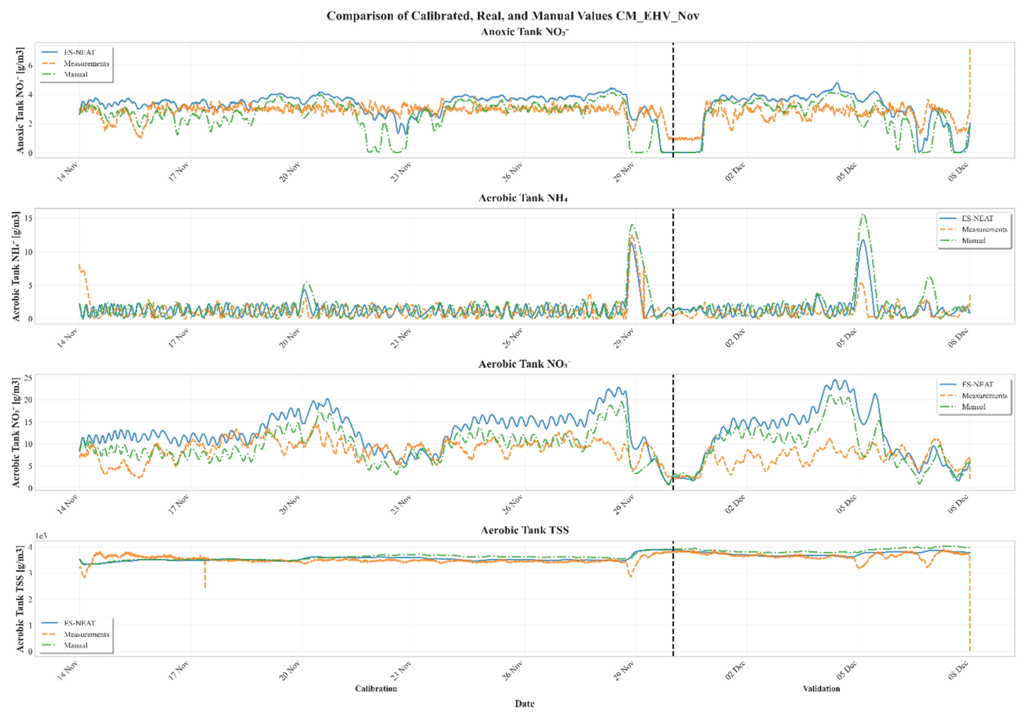
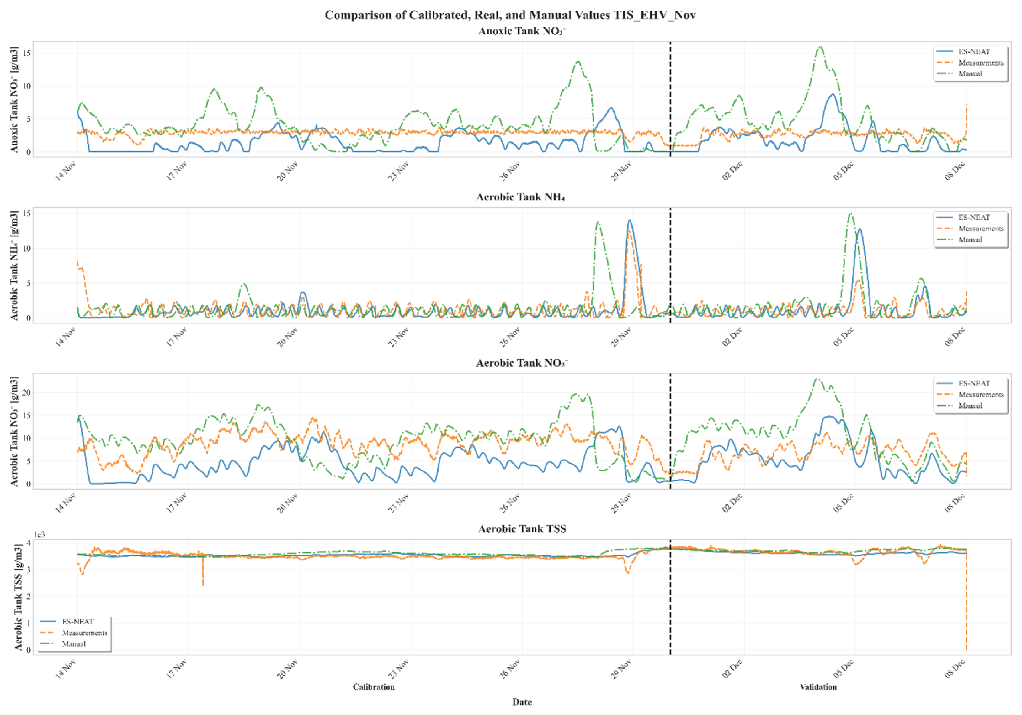
This appendix presents the time-series plots used to evaluate the model’s performance under different calibration scenarios. Each figure compares simulated and reference data for key process variables across the full operational period. The vertical dashed line marks the transition between the calibration (left) and validation (right) phases. All results are plotted using consistent time axes and units to facilitate visual comparison between scenarios.
Figure H1.
Time-series comparisons between observed and simulated effluent concentrations for TSS, NH4+, and NO3− in the aerobic tank and NO3− in the anoxic tank during July 2013 calibration and validation periods (TIS model only).
Figure H1.
Time-series comparisons between observed and simulated effluent concentrations for TSS, NH4+, and NO3− in the aerobic tank and NO3− in the anoxic tank during July 2013 calibration and validation periods (TIS model only).
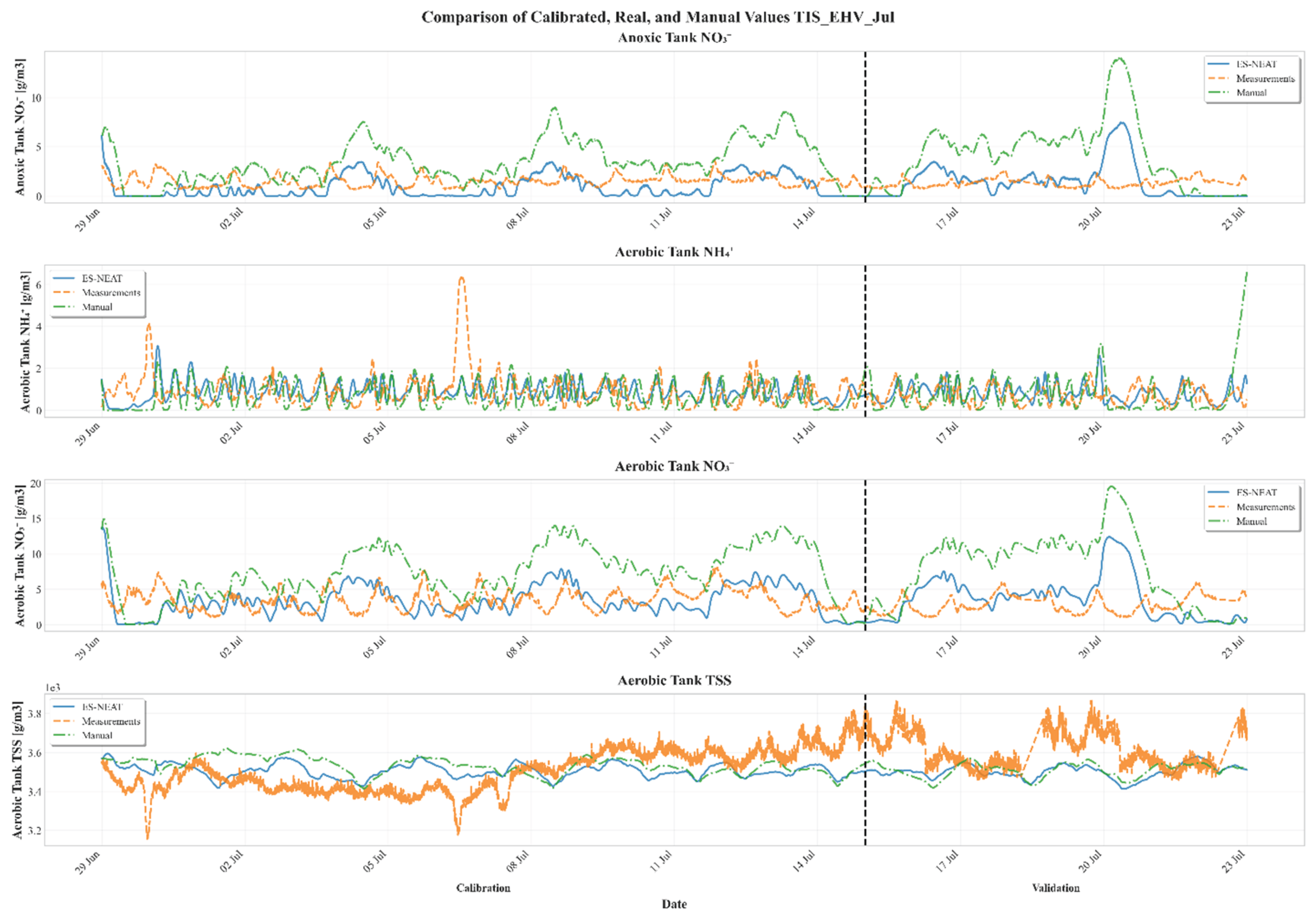
Figure H2.
Time-series comparisons between observed and simulated effluent concentrations for NO3− in the anoxic tank and for NH4+, NO3−, and TSS in the last tank during the September 2013 calibration and validation periods. The left panel corresponds to the CM and the right panel to the TIS model. Results are shown for Manual, PSO (only CM), and ES-NEAT calibration methods.
Figure H2.
Time-series comparisons between observed and simulated effluent concentrations for NO3− in the anoxic tank and for NH4+, NO3−, and TSS in the last tank during the September 2013 calibration and validation periods. The left panel corresponds to the CM and the right panel to the TIS model. Results are shown for Manual, PSO (only CM), and ES-NEAT calibration methods.
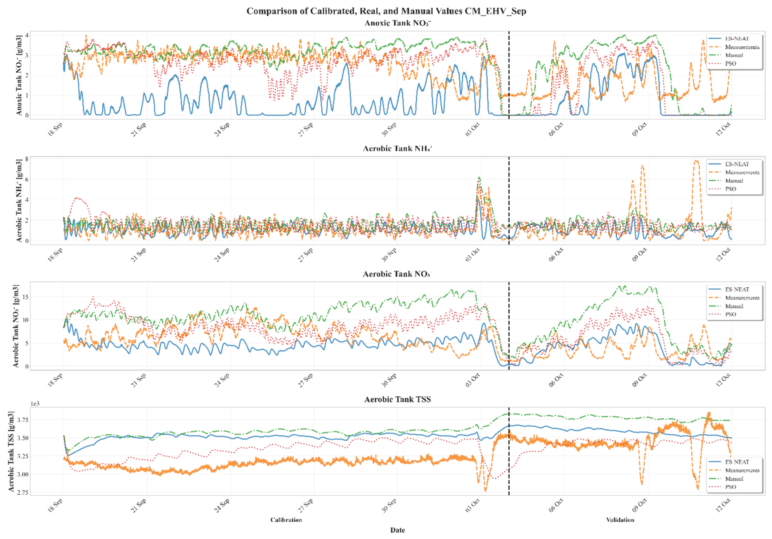
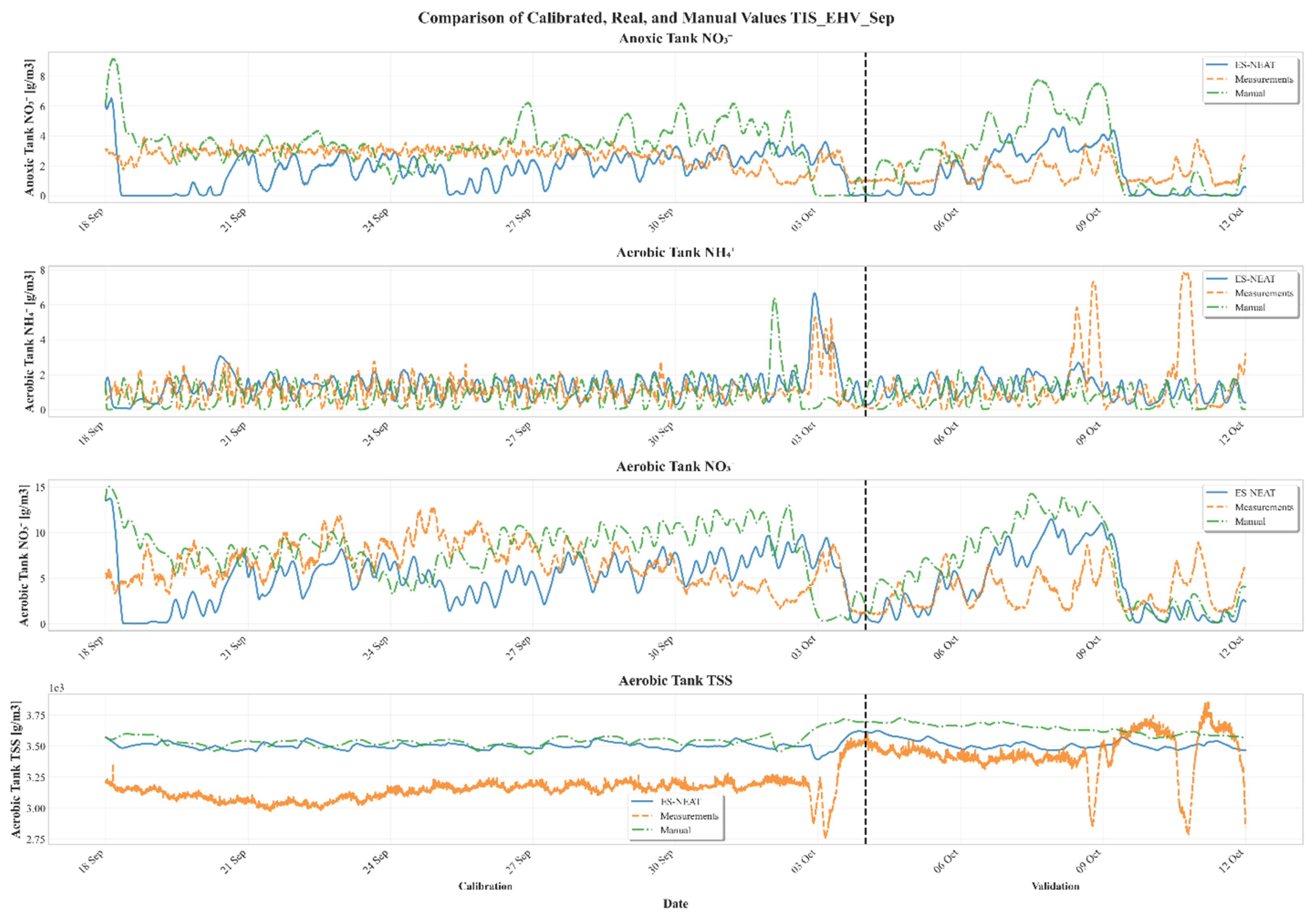
Figure H3.
Time-series comparisons between observed and simulated effluent concentrations for NO3− in the anoxic tank and for NH4+, NO3−, and TSS in the last tank during the November 2013 calibration and validation periods. The left panel corresponds to the CM and the right panel to the TIS model. Results are shown for Manual and ES-NEAT calibration methods.
Figure H3.
Time-series comparisons between observed and simulated effluent concentrations for NO3− in the anoxic tank and for NH4+, NO3−, and TSS in the last tank during the November 2013 calibration and validation periods. The left panel corresponds to the CM and the right panel to the TIS model. Results are shown for Manual and ES-NEAT calibration methods.
Appendix B. Variable-Level Performance Metrics
This appendix presents detailed calibration and validation performance metrics (KGE, R2, RMSE) for each monitored variable (ANOXIC_NO3, LAST_NH4, LAST_NO3, LAST_TSS) across all temporal scenarios (July, September, November) and calibration methods (Manual, PSO, ES-NEAT). Statistics include mean values, standard deviations, and 95% confidence intervals for each scenario-variable-method combination, enabling variable-specific trend identification and assessment of which effluent parameters benefited most from automated calibration approaches.

Table B1.
Variable-level performance metrics for Compartmental Model (CM) across calibration scenarios, methods, and monitoring locations.
Table B1.
Variable-level performance metrics for Compartmental Model (CM) across calibration scenarios, methods, and monitoring locations.
| Scenario | Variable | Period | Method | Metric | Mean | SD | CI_Lower | CI_Upper |
| Jul | ANOXIC_NO3 | Calibration | Manual | KGE | -0.47 | 0.136 | -0.687 | -0.254 |
| Jul | ANOXIC_NO3 | Calibration | NEAT | KGE | -0.368 | 0.219 | -0.717 | -0.019 |
| Jul | ANOXIC_NO3 | Calibration | PSO | KGE | -0.341 | 0.269 | -0.768 | 0.087 |
| Jul | ANOXIC_NO3 | Validation | Manual | KGE | -0.998 | 0.036 | -1.321 | -0.675 |
| Jul | ANOXIC_NO3 | Validation | NEAT | KGE | -1.436 | 0.014 | -1.562 | -1.311 |
| Jul | ANOXIC_NO3 | Validation | PSO | KGE | -1.547 | 0.019 | -1.72 | -1.374 |
| Jul | LAST_NH4 | Calibration | Manual | KGE | -0.013 | 0.084 | -0.147 | 0.12 |
| Jul | LAST_NH4 | Calibration | NEAT | KGE | -0.26 | 0.135 | -0.474 | -0.046 |
| Jul | LAST_NH4 | Calibration | PSO | KGE | -0.046 | 0.111 | -0.223 | 0.13 |
| Jul | LAST_NH4 | Validation | Manual | KGE | -0.187 | 0.103 | -1.108 | 0.735 |
| Jul | LAST_NH4 | Validation | NEAT | KGE | -0.119 | 0.083 | -0.864 | 0.625 |
| Jul | LAST_NH4 | Validation | PSO | KGE | 0.039 | 0.098 | -0.839 | 0.917 |
| Jul | LAST_NO3 | Calibration | Manual | KGE | -0.982 | 0.365 | -1.563 | -0.401 |
| Jul | LAST_NO3 | Calibration | NEAT | KGE | 0.016 | 0.119 | -0.174 | 0.206 |
| Jul | LAST_NO3 | Calibration | PSO | KGE | 0.008 | 0.169 | -0.261 | 0.276 |
| Jul | LAST_NO3 | Validation | Manual | KGE | -2.655 | 0.247 | -4.872 | -0.438 |
| Jul | LAST_NO3 | Validation | NEAT | KGE | -0.779 | 0.009 | -0.864 | -0.693 |
| Jul | LAST_NO3 | Validation | PSO | KGE | -0.905 | 0.058 | -1.424 | -0.386 |
| Jul | LAST_TSS | Calibration | Manual | KGE | 0.202 | 0.14 | -0.021 | 0.424 |
| Jul | LAST_TSS | Calibration | NEAT | KGE | 0.088 | 0.392 | -0.537 | 0.712 |
| Jul | LAST_TSS | Calibration | PSO | KGE | 0.079 | 0.261 | -0.336 | 0.495 |
| Jul | LAST_TSS | Validation | Manual | KGE | -0.097 | 0.238 | -2.24 | 2.046 |
| Jul | LAST_TSS | Validation | NEAT | KGE | 0.107 | 0.004 | 0.073 | 0.142 |
| Jul | LAST_TSS | Validation | PSO | KGE | -0.28 | 0.444 | -4.27 | 3.71 |
| Nov | ANOXIC_NO3 | Calibration | Manual | KGE | -1.563 | 1.458 | -3.883 | 0.758 |
| Nov | ANOXIC_NO3 | Calibration | NEAT | KGE | -0.52 | 0.536 | -1.374 | 0.333 |
| Nov | ANOXIC_NO3 | Validation | Manual | KGE | -0.208 | 0.795 | -7.347 | 6.932 |
| Nov | ANOXIC_NO3 | Validation | NEAT | KGE | -0.264 | 0.587 | -5.535 | 5.006 |
| Nov | LAST_NH4 | Calibration | Manual | KGE | -0.006 | 0.237 | -0.384 | 0.372 |
| Nov | LAST_NH4 | Calibration | NEAT | KGE | 0.24 | 0.41 | -0.412 | 0.892 |
| Nov | LAST_NH4 | Validation | Manual | KGE | -1.051 | 1.298 | -12.712 | 10.61 |
| Nov | LAST_NH4 | Validation | NEAT | KGE | -0.328 | 0.257 | -2.636 | 1.98 |
| Nov | LAST_NO3 | Calibration | Manual | KGE | -0.038 | 0.06 | -0.133 | 0.057 |
| Nov | LAST_NO3 | Calibration | NEAT | KGE | -0.338 | 0.203 | -0.662 | -0.015 |
| Nov | LAST_NO3 | Validation | Manual | KGE | -0.617 | 0.809 | -7.881 | 6.648 |
| Nov | LAST_NO3 | Validation | NEAT | KGE | -1.332 | 0.832 | -8.803 | 6.139 |
| Nov | LAST_TSS | Calibration | Manual | KGE | 0.282 | 0.283 | -0.168 | 0.732 |
| Nov | LAST_TSS | Calibration | NEAT | KGE | 0.253 | 0.279 | -0.191 | 0.698 |
| Nov | LAST_TSS | Validation | Manual | KGE | 0.331 | 0.348 | -2.791 | 3.454 |
| Nov | LAST_TSS | Validation | NEAT | KGE | 0.382 | 0.642 | -5.39 | 6.154 |
| Sep | ANOXIC_NO3 | Calibration | Manual | KGE | -0.08 | 0.036 | -0.137 | -0.022 |
| Sep | ANOXIC_NO3 | Calibration | NEAT | KGE | -0.672 | 0.454 | -1.395 | 0.05 |
| Sep | ANOXIC_NO3 | Calibration | PSO | KGE | -0.31 | 0.416 | -0.973 | 0.352 |
| Sep | ANOXIC_NO3 | Validation | Manual | KGE | -0.391 | 0.073 | -1.046 | 0.265 |
| Sep | ANOXIC_NO3 | Validation | NEAT | KGE | -0.022 | 0.052 | -0.491 | 0.447 |
| Sep | ANOXIC_NO3 | Validation | PSO | KGE | -0.169 | 0.077 | -0.857 | 0.519 |
| Sep | LAST_NH4 | Calibration | Manual | KGE | 0.053 | 0.183 | -0.239 | 0.344 |
| Sep | LAST_NH4 | Calibration | NEAT | KGE | 0.183 | 0.174 | -0.095 | 0.461 |
| Sep | LAST_NH4 | Calibration | PSO | KGE | -0.011 | 0.447 | -0.723 | 0.7 |
| Sep | LAST_NH4 | Validation | Manual | KGE | -0.121 | 0.201 | -1.923 | 1.68 |
| Sep | LAST_NH4 | Validation | NEAT | KGE | -0.022 | 0.218 | -1.984 | 1.941 |
| Sep | LAST_NH4 | Validation | PSO | KGE | -0.13 | 0.009 | -0.21 | -0.051 |
| Sep | LAST_NO3 | Calibration | Manual | KGE | -0.602 | 0.657 | -1.649 | 0.444 |
| Sep | LAST_NO3 | Calibration | NEAT | KGE | -0.066 | 0.327 | -0.587 | 0.455 |
| Sep | LAST_NO3 | Calibration | PSO | KGE | -0.261 | 0.29 | -0.723 | 0.2 |
| Sep | LAST_NO3 | Validation | Manual | KGE | -1.316 | 0.103 | -2.242 | -0.39 |
| Sep | LAST_NO3 | Validation | NEAT | KGE | 0.236 | 0.126 | -0.9 | 1.371 |
| Sep | LAST_NO3 | Validation | PSO | KGE | -0.268 | 0.013 | -0.383 | -0.153 |
| Sep | LAST_TSS | Calibration | Manual | KGE | -0.014 | 0.418 | -0.679 | 0.651 |
| Sep | LAST_TSS | Calibration | NEAT | KGE | -0.316 | 0.514 | -1.133 | 0.502 |
| Sep | LAST_TSS | Calibration | PSO | KGE | -0.202 | 0.524 | -1.037 | 0.632 |
| Sep | LAST_TSS | Validation | Manual | KGE | -0.12 | 0.643 | -5.899 | 5.66 |
| Sep | LAST_TSS | Validation | NEAT | KGE | 0.012 | 0.669 | -6.003 | 6.027 |
| Sep | LAST_TSS | Validation | PSO | KGE | -0.851 | 0.581 | -6.072 | 4.371 |
| Jul | ANOXIC_NO3 | Calibration | Manual | R2 | 0.043 | 0.028 | -0.001 | 0.088 |
| Jul | ANOXIC_NO3 | Calibration | NEAT | R2 | 0.013 | 0.014 | -0.009 | 0.035 |
| Jul | ANOXIC_NO3 | Calibration | PSO | R2 | 0.023 | 0.019 | -0.007 | 0.054 |
| Jul | ANOXIC_NO3 | Validation | Manual | R2 | 0.027 | 0.037 | -0.305 | 0.358 |
| Jul | ANOXIC_NO3 | Validation | NEAT | R2 | 0.083 | 0.059 | -0.443 | 0.608 |
| Jul | ANOXIC_NO3 | Validation | PSO | R2 | 0.08 | 0.113 | -0.932 | 1.092 |
| Jul | LAST_NH4 | Calibration | Manual | R2 | 0.017 | 0.018 | -0.011 | 0.045 |
| Jul | LAST_NH4 | Calibration | NEAT | R2 | 0.022 | 0.018 | -0.007 | 0.05 |
| Jul | LAST_NH4 | Calibration | PSO | R2 | 0.035 | 0.036 | -0.022 | 0.093 |
| Jul | LAST_NH4 | Validation | Manual | R2 | 0.035 | 0.026 | -0.197 | 0.267 |
| Jul | LAST_NH4 | Validation | NEAT | R2 | 0.032 | 0.032 | -0.255 | 0.32 |
| Jul | LAST_NH4 | Validation | PSO | R2 | 0.072 | 0.049 | -0.365 | 0.509 |
| Jul | LAST_NO3 | Calibration | Manual | R2 | 0.088 | 0.07 | -0.024 | 0.2 |
| Jul | LAST_NO3 | Calibration | NEAT | R2 | 0.036 | 0.033 | -0.017 | 0.088 |
| Jul | LAST_NO3 | Calibration | PSO | R2 | 0.061 | 0.068 | -0.048 | 0.169 |
| Jul | LAST_NO3 | Validation | Manual | R2 | 0.058 | 0.081 | -0.669 | 0.785 |
| Jul | LAST_NO3 | Validation | NEAT | R2 | 0.111 | 0.073 | -0.548 | 0.77 |
| Jul | LAST_NO3 | Validation | PSO | R2 | 0.119 | 0.119 | -0.952 | 1.189 |
| Jul | LAST_TSS | Calibration | Manual | R2 | 0.142 | 0.095 | -0.009 | 0.293 |
| Jul | LAST_TSS | Calibration | NEAT | R2 | 0.289 | 0.284 | -0.164 | 0.741 |
| Jul | LAST_TSS | Calibration | PSO | R2 | 0.155 | 0.131 | -0.053 | 0.363 |
| Jul | LAST_TSS | Validation | Manual | R2 | 0.05 | 0.055 | -0.446 | 0.545 |
| Jul | LAST_TSS | Validation | NEAT | R2 | 0.175 | 0.071 | -0.463 | 0.813 |
| Jul | LAST_TSS | Validation | PSO | R2 | 0.131 | 0.101 | -0.78 | 1.043 |
| Nov | ANOXIC_NO3 | Calibration | Manual | R2 | 0.115 | 0.215 | -0.228 | 0.457 |
| Nov | ANOXIC_NO3 | Calibration | NEAT | R2 | 0.142 | 0.259 | -0.27 | 0.553 |
| Nov | ANOXIC_NO3 | Validation | Manual | R2 | 0.517 | 0.316 | -2.319 | 3.353 |
| Nov | ANOXIC_NO3 | Validation | NEAT | R2 | 0.583 | 0.225 | -1.435 | 2.601 |
| Nov | LAST_NH4 | Calibration | Manual | R2 | 0.184 | 0.33 | -0.342 | 0.709 |
| Nov | LAST_NH4 | Calibration | NEAT | R2 | 0.216 | 0.376 | -0.382 | 0.815 |
| Nov | LAST_NH4 | Validation | Manual | R2 | 0.172 | 0.234 | -1.929 | 2.274 |
| Nov | LAST_NH4 | Validation | NEAT | R2 | 0.211 | 0.296 | -2.444 | 2.867 |
| Nov | LAST_NO3 | Calibration | Manual | R2 | 0.172 | 0.146 | -0.061 | 0.405 |
| Nov | LAST_NO3 | Calibration | NEAT | R2 | 0.176 | 0.184 | -0.116 | 0.469 |
| Nov | LAST_NO3 | Validation | Manual | R2 | 0.38 | 0.12 | -0.702 | 1.461 |
| Nov | LAST_NO3 | Validation | NEAT | R2 | 0.399 | 0.138 | -0.839 | 1.637 |
| Nov | LAST_TSS | Calibration | Manual | R2 | 0.225 | 0.246 | -0.167 | 0.617 |
| Nov | LAST_TSS | Calibration | NEAT | R2 | 0.163 | 0.148 | -0.072 | 0.398 |
| Nov | LAST_TSS | Validation | Manual | R2 | 0.414 | 0.429 | -3.44 | 4.269 |
| Nov | LAST_TSS | Validation | NEAT | R2 | 0.385 | 0.507 | -4.173 | 4.942 |
| Sep | ANOXIC_NO3 | Calibration | Manual | R2 | 0.021 | 0.042 | -0.045 | 0.088 |
| Sep | ANOXIC_NO3 | Calibration | NEAT | R2 | 0.022 | 0.032 | -0.029 | 0.073 |
| Sep | ANOXIC_NO3 | Calibration | PSO | R2 | 0.034 | 0.055 | -0.053 | 0.121 |
| Sep | ANOXIC_NO3 | Validation | Manual | R2 | 0.054 | 0.054 | -0.433 | 0.541 |
| Sep | ANOXIC_NO3 | Validation | NEAT | R2 | 0.053 | 0.031 | -0.228 | 0.333 |
| Sep | ANOXIC_NO3 | Validation | PSO | R2 | 0.127 | 0.107 | -0.831 | 1.084 |
| Sep | LAST_NH4 | Calibration | Manual | R2 | 0.175 | 0.333 | -0.355 | 0.705 |
| Sep | LAST_NH4 | Calibration | NEAT | R2 | 0.082 | 0.131 | -0.127 | 0.292 |
| Sep | LAST_NH4 | Calibration | PSO | R2 | 0.131 | 0.256 | -0.276 | 0.538 |
| Sep | LAST_NH4 | Validation | Manual | R2 | 0.097 | 0.104 | -0.833 | 1.027 |
| Sep | LAST_NH4 | Validation | NEAT | R2 | 0.071 | 0.031 | -0.208 | 0.351 |
| Sep | LAST_NH4 | Validation | PSO | R2 | 0.043 | 0.04 | -0.316 | 0.402 |
| Sep | LAST_NO3 | Calibration | Manual | R2 | 0.027 | 0.026 | -0.016 | 0.069 |
| Sep | LAST_NO3 | Calibration | NEAT | R2 | 0.071 | 0.108 | -0.1 | 0.243 |
| Sep | LAST_NO3 | Calibration | PSO | R2 | 0.073 | 0.106 | -0.096 | 0.242 |
| Sep | LAST_NO3 | Validation | Manual | R2 | 0.118 | 0.096 | -0.747 | 0.983 |
| Sep | LAST_NO3 | Validation | NEAT | R2 | 0.166 | 0.106 | -0.786 | 1.119 |
| Sep | LAST_NO3 | Validation | PSO | R2 | 0.192 | 0.061 | -0.353 | 0.738 |
| Sep | LAST_TSS | Calibration | Manual | R2 | 0.225 | 0.174 | -0.053 | 0.502 |
| Sep | LAST_TSS | Calibration | NEAT | R2 | 0.33 | 0.301 | -0.148 | 0.809 |
| Sep | LAST_TSS | Calibration | PSO | R2 | 0.213 | 0.113 | 0.033 | 0.392 |
| Sep | LAST_TSS | Validation | Manual | R2 | 0.238 | 0.226 | -1.793 | 2.269 |
| Sep | LAST_TSS | Validation | NEAT | R2 | 0.266 | 0.34 | -2.788 | 3.32 |
| Sep | LAST_TSS | Validation | PSO | R2 | 0.33 | 0.441 | -3.631 | 4.292 |
| Jul | ANOXIC_NO3 | Calibration | Manual | RMSE | 1.586 | 0.132 | 1.376 | 1.796 |
| Jul | ANOXIC_NO3 | Calibration | NEAT | RMSE | 1.455 | 0.08 | 1.328 | 1.581 |
| Jul | ANOXIC_NO3 | Calibration | PSO | RMSE | 1.407 | 0.096 | 1.255 | 1.559 |
| Jul | ANOXIC_NO3 | Validation | Manual | RMSE | 2.272 | 0.088 | 1.485 | 3.058 |
| Jul | ANOXIC_NO3 | Validation | NEAT | RMSE | 1.453 | 0.038 | 1.114 | 1.793 |
| Jul | ANOXIC_NO3 | Validation | PSO | RMSE | 1.471 | 0.034 | 1.169 | 1.772 |
| Jul | LAST_NH4 | Calibration | Manual | RMSE | 1.022 | 0.222 | 0.668 | 1.376 |
| Jul | LAST_NH4 | Calibration | NEAT | RMSE | 1.075 | 0.303 | 0.592 | 1.557 |
| Jul | LAST_NH4 | Calibration | PSO | RMSE | 0.966 | 0.272 | 0.533 | 1.398 |
| Jul | LAST_NH4 | Validation | Manual | RMSE | 0.825 | 0.069 | 0.21 | 1.441 |
| Jul | LAST_NH4 | Validation | NEAT | RMSE | 0.745 | 0.04 | 0.389 | 1.101 |
| Jul | LAST_NH4 | Validation | PSO | RMSE | 0.683 | 0.06 | 0.146 | 1.22 |
| Jul | LAST_NO3 | Calibration | Manual | RMSE | 5.883 | 1.389 | 3.672 | 8.093 |
| Jul | LAST_NO3 | Calibration | NEAT | RMSE | 2.183 | 0.396 | 1.553 | 2.813 |
| Jul | LAST_NO3 | Calibration | PSO | RMSE | 2.177 | 0.297 | 1.704 | 2.65 |
| Jul | LAST_NO3 | Validation | Manual | RMSE | 9.875 | 0.891 | 1.87 | 17.881 |
| Jul | LAST_NO3 | Validation | NEAT | RMSE | 3.716 | 0.253 | 1.441 | 5.991 |
| Jul | LAST_NO3 | Validation | PSO | RMSE | 4.12 | 0.52 | -0.551 | 8.79 |
| Jul | LAST_TSS | Calibration | Manual | RMSE | 120.484 | 43.606 | 51.097 | 189.872 |
| Jul | LAST_TSS | Calibration | NEAT | RMSE | 177.559 | 111.135 | 0.719 | 354.399 |
| Jul | LAST_TSS | Calibration | PSO | RMSE | 107.442 | 28.792 | 61.628 | 153.256 |
| Jul | LAST_TSS | Validation | Manual | RMSE | 133.965 | 14.904 | 0.056 | 267.874 |
| Jul | LAST_TSS | Validation | NEAT | RMSE | 155.082 | 3.123 | 127.026 | 183.137 |
| Jul | LAST_TSS | Validation | PSO | RMSE | 145.49 | 20.36 | -37.435 | 328.414 |
| Nov | ANOXIC_NO3 | Calibration | Manual | RMSE | 1.028 | 0.244 | 0.639 | 1.416 |
| Nov | ANOXIC_NO3 | Calibration | NEAT | RMSE | 0.828 | 0.128 | 0.625 | 1.032 |
| Nov | ANOXIC_NO3 | Validation | Manual | RMSE | 1.084 | 0.435 | -2.824 | 4.993 |
| Nov | ANOXIC_NO3 | Validation | NEAT | RMSE | 1.091 | 0.067 | 0.486 | 1.696 |
| Nov | LAST_NH4 | Calibration | Manual | RMSE | 1.566 | 0.482 | 0.799 | 2.333 |
| Nov | LAST_NH4 | Calibration | NEAT | RMSE | 1.167 | 0.338 | 0.628 | 1.705 |
| Nov | LAST_NH4 | Validation | Manual | RMSE | 2.457 | 2.013 | -15.631 | 20.544 |
| Nov | LAST_NH4 | Validation | NEAT | RMSE | 1.584 | 0.874 | -6.269 | 9.437 |
| Nov | LAST_NO3 | Calibration | Manual | RMSE | 3.239 | 0.694 | 2.134 | 4.344 |
| Nov | LAST_NO3 | Calibration | NEAT | RMSE | 5.354 | 1.122 | 3.569 | 7.139 |
| Nov | LAST_NO3 | Validation | Manual | RMSE | 5.234 | 0.449 | 1.197 | 9.271 |
| Nov | LAST_NO3 | Validation | NEAT | RMSE | 7.617 | 0.464 | 3.448 | 11.786 |
| Nov | LAST_TSS | Calibration | Manual | RMSE | 177.937 | 51.278 | 96.343 | 259.532 |
| Nov | LAST_TSS | Calibration | NEAT | RMSE | 144.327 | 56.155 | 54.972 | 233.681 |
| Nov | LAST_TSS | Validation | Manual | RMSE | 256.23 | 140.957 | -1010.22 | 1522.677 |
| Nov | LAST_TSS | Validation | NEAT | RMSE | 156.471 | 149.071 | -1182.88 | 1495.816 |
| Sep | ANOXIC_NO3 | Calibration | Manual | RMSE | 0.823 | 0.604 | -0.138 | 1.784 |
| Sep | ANOXIC_NO3 | Calibration | NEAT | RMSE | 2.171 | 0.561 | 1.278 | 3.064 |
| Sep | ANOXIC_NO3 | Calibration | PSO | RMSE | 0.907 | 0.302 | 0.426 | 1.387 |
| Sep | ANOXIC_NO3 | Validation | Manual | RMSE | 1.703 | 0.173 | 0.145 | 3.262 |
| Sep | ANOXIC_NO3 | Validation | NEAT | RMSE | 1.381 | 0.077 | 0.685 | 2.077 |
| Sep | ANOXIC_NO3 | Validation | PSO | RMSE | 1.401 | 0.307 | -1.354 | 4.156 |
| Sep | LAST_NH4 | Calibration | Manual | RMSE | 0.87 | 0.122 | 0.675 | 1.065 |
| Sep | LAST_NH4 | Calibration | NEAT | RMSE | 0.713 | 0.146 | 0.48 | 0.945 |
| Sep | LAST_NH4 | Calibration | PSO | RMSE | 0.997 | 0.324 | 0.482 | 1.512 |
| Sep | LAST_NH4 | Validation | Manual | RMSE | 1.51 | 0.758 | -5.302 | 8.322 |
| Sep | LAST_NH4 | Validation | NEAT | RMSE | 1.508 | 1.16 | -8.913 | 11.929 |
| Sep | LAST_NH4 | Validation | PSO | RMSE | 1.525 | 0.926 | -6.797 | 9.848 |
| Sep | LAST_NO3 | Calibration | Manual | RMSE | 5.633 | 2.759 | 1.243 | 10.023 |
| Sep | LAST_NO3 | Calibration | NEAT | RMSE | 3.251 | 1.461 | 0.926 | 5.576 |
| Sep | LAST_NO3 | Calibration | PSO | RMSE | 4.005 | 1.955 | 0.894 | 7.116 |
| Sep | LAST_NO3 | Validation | Manual | RMSE | 7.178 | 0.473 | 2.929 | 11.427 |
| Sep | LAST_NO3 | Validation | NEAT | RMSE | 2.785 | 0.839 | -4.757 | 10.327 |
| Sep | LAST_NO3 | Validation | PSO | RMSE | 4.102 | 0.515 | -0.523 | 8.726 |
| Sep | LAST_TSS | Calibration | Manual | RMSE | 436.808 | 29.651 | 389.627 | 483.989 |
| Sep | LAST_TSS | Calibration | NEAT | RMSE | 378.341 | 31.405 | 328.369 | 428.313 |
| Sep | LAST_TSS | Calibration | PSO | RMSE | 233.916 | 74.026 | 116.125 | 351.707 |
| Sep | LAST_TSS | Validation | Manual | RMSE | 371.807 | 2.454 | 349.76 | 393.854 |
| Sep | LAST_TSS | Validation | NEAT | RMSE | 228.335 | 30.557 | -46.211 | 502.881 |
| Sep | LAST_TSS | Validation | PSO | RMSE | 191.352 | 65.815 | -399.968 | 782.673 |
Table B2.
Variable-level performance metrics for Tank-in-Series Model (TIS) across calibration scenarios, methods, and monitoring locations.
Table B2.
Variable-level performance metrics for Tank-in-Series Model (TIS) across calibration scenarios, methods, and monitoring locations.
| Scenario | Variable | Period | Method | Metric | Mean | SD | CI_Lower | CI_Upper |
| Jul | ANOXIC_NO3 | Calibration | Manual | KGE | -1.923 | 1.146 | -3.748 | -0.099 |
| Jul | ANOXIC_NO3 | Calibration | NEAT | KGE | -0.403 | 0.249 | -0.798 | -0.007 |
| Jul | ANOXIC_NO3 | Validation | Manual | KGE | -6.37 | 3.778 | -40.312 | 27.573 |
| Jul | ANOXIC_NO3 | Validation | NEAT | KGE | -2.266 | 2.179 | -21.846 | 17.313 |
| Jul | LAST_NH4 | Calibration | Manual | KGE | 0.042 | 0.254 | -0.362 | 0.445 |
| Jul | LAST_NH4 | Calibration | NEAT | KGE | -0.056 | 0.095 | -0.206 | 0.095 |
| Jul | LAST_NH4 | Validation | Manual | KGE | -0.443 | 0.939 | -8.88 | 7.994 |
| Jul | LAST_NH4 | Validation | NEAT | KGE | 0.243 | 0.092 | -0.583 | 1.07 |
| Jul | LAST_NO3 | Calibration | Manual | KGE | -0.968 | 0.252 | -1.369 | -0.567 |
| Jul | LAST_NO3 | Calibration | NEAT | KGE | -0.072 | 0.141 | -0.296 | 0.152 |
| Jul | LAST_NO3 | Validation | Manual | KGE | -2.885 | 1.348 | -14.997 | 9.227 |
| Jul | LAST_NO3 | Validation | NEAT | KGE | -0.965 | 1.121 | -11.039 | 9.109 |
| Jul | LAST_TSS | Calibration | Manual | KGE | 0.111 | 0.165 | -0.151 | 0.372 |
| Jul | LAST_TSS | Calibration | NEAT | KGE | 0.035 | 0.118 | -0.153 | 0.223 |
| Jul | LAST_TSS | Validation | Manual | KGE | -0.179 | 0.147 | -1.495 | 1.137 |
| Jul | LAST_TSS | Validation | NEAT | KGE | -0.114 | 0.058 | -0.634 | 0.406 |
| Nov | ANOXIC_NO3 | Calibration | Manual | KGE | -5.624 | 4.183 | -12.28 | 1.031 |
| Nov | ANOXIC_NO3 | Calibration | NEAT | KGE | -2.402 | 1.776 | -5.228 | 0.424 |
| Nov | ANOXIC_NO3 | Validation | Manual | KGE | -3.709 | 2.894 | -29.714 | 22.296 |
| Nov | ANOXIC_NO3 | Validation | NEAT | KGE | -1.272 | 2.264 | -21.615 | 19.071 |
| Nov | LAST_NH4 | Calibration | Manual | KGE | -0.062 | 0.25 | -0.46 | 0.336 |
| Nov | LAST_NH4 | Calibration | NEAT | KGE | 0.332 | 0.465 | -0.408 | 1.071 |
| Nov | LAST_NH4 | Validation | Manual | KGE | -0.887 | 1.199 | -11.658 | 9.885 |
| Nov | LAST_NH4 | Validation | NEAT | KGE | -0.351 | 0.681 | -6.474 | 5.771 |
| Nov | LAST_NO3 | Calibration | Manual | KGE | -0.261 | 0.514 | -1.079 | 0.558 |
| Nov | LAST_NO3 | Calibration | NEAT | KGE | 0.168 | 0.005 | 0.16 | 0.176 |
| Nov | LAST_NO3 | Validation | Manual | KGE | -0.783 | 0.579 | -5.984 | 4.417 |
| Nov | LAST_NO3 | Validation | NEAT | KGE | -0.025 | 0.72 | -6.495 | 6.444 |
| Nov | LAST_TSS | Calibration | Manual | KGE | 0.1 | 0.364 | -0.479 | 0.679 |
| Nov | LAST_TSS | Calibration | NEAT | KGE | 0.079 | 0.528 | -0.76 | 0.919 |
| Nov | LAST_TSS | Validation | Manual | KGE | 0.202 | 0.247 | -2.022 | 2.425 |
| Nov | LAST_TSS | Validation | NEAT | KGE | 0.375 | 0.49 | -4.031 | 4.781 |
| Sep | ANOXIC_NO3 | Calibration | Manual | KGE | -1.548 | 0.636 | -2.56 | -0.535 |
| Sep | ANOXIC_NO3 | Calibration | NEAT | KGE | -1.091 | 1.081 | -2.81 | 0.628 |
| Sep | ANOXIC_NO3 | Validation | Manual | KGE | -1.361 | 0.027 | -1.602 | -1.121 |
| Sep | ANOXIC_NO3 | Validation | NEAT | KGE | -0.231 | 0.077 | -0.921 | 0.459 |
| Sep | LAST_NH4 | Calibration | Manual | KGE | -0.179 | 0.108 | -0.35 | -0.008 |
| Sep | LAST_NH4 | Calibration | NEAT | KGE | 0.239 | 0.152 | -0.003 | 0.481 |
| Sep | LAST_NH4 | Validation | Manual | KGE | -0.3 | 0.064 | -0.874 | 0.274 |
| Sep | LAST_NH4 | Validation | NEAT | KGE | -0.005 | 0.057 | -0.515 | 0.505 |
| Sep | LAST_NO3 | Calibration | Manual | KGE | -0.508 | 0.481 | -1.275 | 0.258 |
| Sep | LAST_NO3 | Calibration | NEAT | KGE | -0.024 | 0.254 | -0.428 | 0.38 |
| Sep | LAST_NO3 | Validation | Manual | KGE | -0.655 | 0.321 | -3.538 | 2.229 |
| Sep | LAST_NO3 | Validation | NEAT | KGE | -0.095 | 0.076 | -0.773 | 0.584 |
| Sep | LAST_TSS | Calibration | Manual | KGE | 0.051 | 0.331 | -0.475 | 0.577 |
| Sep | LAST_TSS | Calibration | NEAT | KGE | -0.073 | 0.368 | -0.659 | 0.512 |
| Sep | LAST_TSS | Validation | Manual | KGE | -0.244 | 0.604 | -5.674 | 5.185 |
| Sep | LAST_TSS | Validation | NEAT | KGE | 0.324 | 0.606 | -5.125 | 5.772 |
| Jul | ANOXIC_NO3 | Calibration | Manual | R2 | 0.01 | 0.008 | -0.003 | 0.023 |
| Jul | ANOXIC_NO3 | Calibration | NEAT | R2 | 0.009 | 0.01 | -0.007 | 0.025 |
| Jul | ANOXIC_NO3 | Validation | Manual | R2 | 0.187 | 0.211 | -1.713 | 2.087 |
| Jul | ANOXIC_NO3 | Validation | NEAT | R2 | 0.117 | 0.158 | -1.304 | 1.539 |
| Jul | LAST_NH4 | Calibration | Manual | R2 | 0.067 | 0.05 | -0.012 | 0.147 |
| Jul | LAST_NH4 | Calibration | NEAT | R2 | 0.029 | 0.033 | -0.023 | 0.081 |
| Jul | LAST_NH4 | Validation | Manual | R2 | 0.059 | 0.073 | -0.594 | 0.713 |
| Jul | LAST_NH4 | Validation | NEAT | R2 | 0.089 | 0.077 | -0.604 | 0.782 |
| Jul | LAST_NO3 | Calibration | Manual | R2 | 0.024 | 0.03 | -0.024 | 0.071 |
| Jul | LAST_NO3 | Calibration | NEAT | R2 | 0.012 | 0.021 | -0.021 | 0.046 |
| Jul | LAST_NO3 | Validation | Manual | R2 | 0.259 | 0.238 | -1.88 | 2.398 |
| Jul | LAST_NO3 | Validation | NEAT | R2 | 0.161 | 0.214 | -1.762 | 2.084 |
| Jul | LAST_TSS | Calibration | Manual | R2 | 0.089 | 0.138 | -0.131 | 0.309 |
| Jul | LAST_TSS | Calibration | NEAT | R2 | 0.035 | 0.035 | -0.02 | 0.09 |
| Jul | LAST_TSS | Validation | Manual | R2 | 0.023 | 0.002 | 0.008 | 0.039 |
| Jul | LAST_TSS | Validation | NEAT | R2 | 0.008 | 0.004 | -0.028 | 0.044 |
| Nov | ANOXIC_NO3 | Calibration | Manual | R2 | 0.069 | 0.078 | -0.056 | 0.194 |
| Nov | ANOXIC_NO3 | Calibration | NEAT | R2 | 0.058 | 0.066 | -0.046 | 0.163 |
| Nov | ANOXIC_NO3 | Validation | Manual | R2 | 0.131 | 0.001 | 0.118 | 0.143 |
| Nov | ANOXIC_NO3 | Validation | NEAT | R2 | 0.247 | 0.19 | -1.461 | 1.954 |
| Nov | LAST_NH4 | Calibration | Manual | R2 | 0.033 | 0.011 | 0.015 | 0.05 |
| Nov | LAST_NH4 | Calibration | NEAT | R2 | 0.365 | 0.331 | -0.161 | 0.891 |
| Nov | LAST_NH4 | Validation | Manual | R2 | 0.128 | 0.17 | -1.4 | 1.656 |
| Nov | LAST_NH4 | Validation | NEAT | R2 | 0.263 | 0.333 | -2.725 | 3.252 |
| Nov | LAST_NO3 | Calibration | Manual | R2 | 0.186 | 0.163 | -0.073 | 0.445 |
| Nov | LAST_NO3 | Calibration | NEAT | R2 | 0.236 | 0.037 | 0.177 | 0.294 |
| Nov | LAST_NO3 | Validation | Manual | R2 | 0.287 | 0.088 | -0.504 | 1.077 |
| Nov | LAST_NO3 | Validation | NEAT | R2 | 0.337 | 0.027 | 0.09 | 0.583 |
| Nov | LAST_TSS | Calibration | Manual | R2 | 0.09 | 0.07 | -0.022 | 0.201 |
| Nov | LAST_TSS | Calibration | NEAT | R2 | 0.233 | 0.252 | -0.169 | 0.634 |
| Nov | LAST_TSS | Validation | Manual | R2 | 0.369 | 0.323 | -2.531 | 3.27 |
| Nov | LAST_TSS | Validation | NEAT | R2 | 0.519 | 0.389 | -2.974 | 4.012 |
| Sep | ANOXIC_NO3 | Calibration | Manual | R2 | 0.031 | 0.043 | -0.038 | 0.099 |
| Sep | ANOXIC_NO3 | Calibration | NEAT | R2 | 0.04 | 0.039 | -0.022 | 0.101 |
| Sep | ANOXIC_NO3 | Validation | Manual | R2 | 0.133 | 0.03 | -0.137 | 0.402 |
| Sep | ANOXIC_NO3 | Validation | NEAT | R2 | 0.141 | 0.087 | -0.643 | 0.925 |
| Sep | LAST_NH4 | Calibration | Manual | R2 | 0.025 | 0.015 | 0.001 | 0.049 |
| Sep | LAST_NH4 | Calibration | NEAT | R2 | 0.205 | 0.305 | -0.279 | 0.69 |
| Sep | LAST_NH4 | Validation | Manual | R2 | 0.067 | 0.053 | -0.408 | 0.541 |
| Sep | LAST_NH4 | Validation | NEAT | R2 | 0.115 | 0.044 | -0.282 | 0.511 |
| Sep | LAST_NO3 | Calibration | Manual | R2 | 0.056 | 0.042 | -0.011 | 0.123 |
| Sep | LAST_NO3 | Calibration | NEAT | R2 | 0.077 | 0.073 | -0.04 | 0.194 |
| Sep | LAST_NO3 | Validation | Manual | R2 | 0.113 | 0.038 | -0.23 | 0.455 |
| Sep | LAST_NO3 | Validation | NEAT | R2 | 0.182 | 0.085 | -0.584 | 0.949 |
| Sep | LAST_TSS | Calibration | Manual | R2 | 0.14 | 0.18 | -0.146 | 0.426 |
| Sep | LAST_TSS | Calibration | NEAT | R2 | 0.245 | 0.254 | -0.16 | 0.65 |
| Sep | LAST_TSS | Validation | Manual | R2 | 0.167 | 0.002 | 0.146 | 0.188 |
| Sep | LAST_TSS | Validation | NEAT | R2 | 0.35 | 0.32 | -2.527 | 3.226 |
| Jul | ANOXIC_NO3 | Calibration | Manual | RMSE | 2.821 | 0.759 | 1.614 | 4.029 |
| Jul | ANOXIC_NO3 | Calibration | NEAT | RMSE | 1.348 | 0.083 | 1.216 | 1.48 |
| Jul | ANOXIC_NO3 | Validation | Manual | RMSE | 4.492 | 1.441 | -8.452 | 17.436 |
| Jul | ANOXIC_NO3 | Validation | NEAT | RMSE | 1.786 | 1.021 | -7.385 | 10.957 |
| Jul | LAST_NH4 | Calibration | Manual | RMSE | 0.932 | 0.316 | 0.429 | 1.436 |
| Jul | LAST_NH4 | Calibration | NEAT | RMSE | 0.873 | 0.291 | 0.41 | 1.336 |
| Jul | LAST_NH4 | Validation | Manual | RMSE | 0.923 | 0.467 | -3.269 | 5.114 |
| Jul | LAST_NH4 | Validation | NEAT | RMSE | 0.517 | 0.056 | 0.018 | 1.016 |
| Jul | LAST_NO3 | Calibration | Manual | RMSE | 5.392 | 1.125 | 3.602 | 7.183 |
| Jul | LAST_NO3 | Calibration | NEAT | RMSE | 2.516 | 0.269 | 2.088 | 2.943 |
| Jul | LAST_NO3 | Validation | Manual | RMSE | 7.471 | 1.37 | -4.834 | 19.776 |
| Jul | LAST_NO3 | Validation | NEAT | RMSE | 3.532 | 1.615 | -10.979 | 18.043 |
| Jul | LAST_TSS | Calibration | Manual | RMSE | 122.193 | 37.477 | 62.559 | 181.827 |
| Jul | LAST_TSS | Calibration | NEAT | RMSE | 107.589 | 19.198 | 77.041 | 138.137 |
| Jul | LAST_TSS | Validation | Manual | RMSE | 143.35 | 14.828 | 10.127 | 276.572 |
| Jul | LAST_TSS | Validation | NEAT | RMSE | 146.485 | 1.829 | 130.054 | 162.916 |
| Nov | ANOXIC_NO3 | Calibration | Manual | RMSE | 2.829 | 1.075 | 1.118 | 4.54 |
| Nov | ANOXIC_NO3 | Calibration | NEAT | RMSE | 2.073 | 0.244 | 1.685 | 2.462 |
| Nov | ANOXIC_NO3 | Validation | Manual | RMSE | 4.126 | 0.013 | 4.008 | 4.244 |
| Nov | ANOXIC_NO3 | Validation | NEAT | RMSE | 1.861 | 0.98 | -6.94 | 10.662 |
| Nov | LAST_NH4 | Calibration | Manual | RMSE | 2.049 | 1.652 | -0.58 | 4.679 |
| Nov | LAST_NH4 | Calibration | NEAT | RMSE | 1.158 | 0.564 | 0.261 | 2.055 |
| Nov | LAST_NH4 | Validation | Manual | RMSE | 2.325 | 1.952 | -15.217 | 19.867 |
| Nov | LAST_NH4 | Validation | NEAT | RMSE | 1.607 | 1.259 | -9.706 | 12.919 |
| Nov | LAST_NO3 | Calibration | Manual | RMSE | 4.292 | 1.113 | 2.52 | 6.064 |
| Nov | LAST_NO3 | Calibration | NEAT | RMSE | 5.129 | 0.213 | 4.79 | 5.468 |
| Nov | LAST_NO3 | Validation | Manual | RMSE | 6.247 | 1.346 | -5.85 | 18.343 |
| Nov | LAST_NO3 | Validation | NEAT | RMSE | 3.439 | 1.385 | -9.001 | 15.88 |
| Nov | LAST_TSS | Calibration | Manual | RMSE | 172.79 | 37.397 | 113.283 | 232.297 |
| Nov | LAST_TSS | Calibration | NEAT | RMSE | 119.319 | 55.946 | 30.297 | 208.34 |
| Nov | LAST_TSS | Validation | Manual | RMSE | 141.745 | 119.131 | -928.6 | 1212.091 |
| Nov | LAST_TSS | Validation | NEAT | RMSE | 132.24 | 107.92 | -837.386 | 1101.865 |
| Sep | ANOXIC_NO3 | Calibration | Manual | RMSE | 1.633 | 0.73 | 0.471 | 2.794 |
| Sep | ANOXIC_NO3 | Calibration | NEAT | RMSE | 1.541 | 0.556 | 0.656 | 2.426 |
| Sep | ANOXIC_NO3 | Validation | Manual | RMSE | 2.587 | 0.152 | 1.224 | 3.95 |
| Sep | ANOXIC_NO3 | Validation | NEAT | RMSE | 1.437 | 0.301 | -1.266 | 4.139 |
| Sep | LAST_NH4 | Calibration | Manual | RMSE | 1.111 | 0.409 | 0.46 | 1.762 |
| Sep | LAST_NH4 | Calibration | NEAT | RMSE | 0.769 | 0.139 | 0.548 | 0.99 |
| Sep | LAST_NH4 | Validation | Manual | RMSE | 1.667 | 1.059 | -7.849 | 11.182 |
| Sep | LAST_NH4 | Validation | NEAT | RMSE | 1.5 | 0.963 | -7.15 | 10.149 |
| Sep | LAST_NO3 | Calibration | Manual | RMSE | 4.096 | 1.497 | 1.714 | 6.477 |
| Sep | LAST_NO3 | Calibration | NEAT | RMSE | 3.601 | 0.898 | 2.172 | 5.029 |
| Sep | LAST_NO3 | Validation | Manual | RMSE | 5.198 | 0.619 | -0.36 | 10.755 |
| Sep | LAST_NO3 | Validation | NEAT | RMSE | 3.476 | 0.528 | -1.271 | 8.222 |
| Sep | LAST_TSS | Calibration | Manual | RMSE | 407.389 | 35.31 | 351.203 | 463.575 |
| Sep | LAST_TSS | Calibration | NEAT | RMSE | 364.218 | 47.415 | 288.77 | 439.665 |
| Sep | LAST_TSS | Validation | Manual | RMSE | 265.179 | 17.207 | 110.583 | 419.776 |
| Sep | LAST_TSS | Validation | NEAT | RMSE | 166.267 | 85.339 | -600.47 | 933.003 |
Appendix C. Transfer Learning Effectiveness Analysis
This appendix quantifies transfer learning effectiveness through correlation analysis of sequential recalibrations (July→September→November). For each variable and performance metric, Pearson correlation coefficients assess whether progressive improvements occurred across recalibration episodes. Statistical significance (FDR-corrected p-values) and interpretation classifications distinguish variables exhibiting cumulative learning benefits from those constrained by structural limitations. Analysis assumes standalone recalibrations without transfer learning would require computational time equivalent to July baseline scenarios.
Table C1.
Transfer learning correlation analysis for Compartmental Model (CM) showing variable-specific progressive improvement patterns.
Table C1.
Transfer learning correlation analysis for Compartmental Model (CM) showing variable-specific progressive improvement patterns.
| Scenario | Variable | Period | Method | Metric | Mean | SD | CI_Lower | CI_Upper |
| Jul | ANOXIC_NO3 | Calibration | Manual | KGE | -0.470 | 0.136 | -0.687 | -0.254 |
| Jul | ANOXIC_NO3 | Calibration | NEAT | KGE | -0.368 | 0.219 | -0.717 | -0.019 |
| Jul | ANOXIC_NO3 | Calibration | PSO | KGE | -0.341 | 0.269 | -0.768 | 0.087 |
| Jul | ANOXIC_NO3 | Validation | Manual | KGE | -0.998 | 0.036 | -1.321 | -0.675 |
| Jul | ANOXIC_NO3 | Validation | NEAT | KGE | -1.436 | 0.014 | -1.562 | -1.311 |
| Jul | ANOXIC_NO3 | Validation | PSO | KGE | -1.547 | 0.019 | -1.720 | -1.374 |
| Jul | LAST_NH4 | Calibration | Manual | KGE | -0.013 | 0.084 | -0.147 | 0.120 |
| Jul | LAST_NH4 | Calibration | NEAT | KGE | -0.260 | 0.135 | -0.474 | -0.046 |
| Jul | LAST_NH4 | Calibration | PSO | KGE | -0.046 | 0.111 | -0.223 | 0.130 |
| Jul | LAST_NH4 | Validation | Manual | KGE | -0.187 | 0.103 | -1.108 | 0.735 |
| Jul | LAST_NH4 | Validation | NEAT | KGE | -0.119 | 0.083 | -0.864 | 0.625 |
| Jul | LAST_NH4 | Validation | PSO | KGE | 0.039 | 0.098 | -0.839 | 0.917 |
| Jul | LAST_NO3 | Calibration | Manual | KGE | -0.982 | 0.365 | -1.563 | -0.401 |
| Jul | LAST_NO3 | Calibration | NEAT | KGE | 0.016 | 0.119 | -0.174 | 0.206 |
| Jul | LAST_NO3 | Calibration | PSO | KGE | 0.008 | 0.169 | -0.261 | 0.276 |
| Jul | LAST_NO3 | Validation | Manual | KGE | -2.655 | 0.247 | -4.872 | -0.438 |
| Jul | LAST_NO3 | Validation | NEAT | KGE | -0.779 | 0.009 | -0.864 | -0.693 |
| Jul | LAST_NO3 | Validation | PSO | KGE | -0.905 | 0.058 | -1.424 | -0.386 |
| Jul | LAST_TSS | Calibration | Manual | KGE | 0.202 | 0.140 | -0.021 | 0.424 |
| Jul | LAST_TSS | Calibration | NEAT | KGE | 0.088 | 0.392 | -0.537 | 0.712 |
| Jul | LAST_TSS | Calibration | PSO | KGE | 0.079 | 0.261 | -0.336 | 0.495 |
| Jul | LAST_TSS | Validation | Manual | KGE | -0.097 | 0.238 | -2.240 | 2.046 |
| Jul | LAST_TSS | Validation | NEAT | KGE | 0.107 | 0.004 | 0.073 | 0.142 |
| Jul | LAST_TSS | Validation | PSO | KGE | -0.280 | 0.444 | -4.270 | 3.710 |
| Nov | ANOXIC_NO3 | Calibration | Manual | KGE | -1.563 | 1.458 | -3.883 | 0.758 |
| Nov | ANOXIC_NO3 | Calibration | NEAT | KGE | -0.520 | 0.536 | -1.374 | 0.333 |
| Nov | ANOXIC_NO3 | Validation | Manual | KGE | -0.208 | 0.795 | -7.347 | 6.932 |
| Nov | ANOXIC_NO3 | Validation | NEAT | KGE | -0.264 | 0.587 | -5.535 | 5.006 |
| Nov | LAST_NH4 | Calibration | Manual | KGE | -0.006 | 0.237 | -0.384 | 0.372 |
| Nov | LAST_NH4 | Calibration | NEAT | KGE | 0.240 | 0.410 | -0.412 | 0.892 |
| Nov | LAST_NH4 | Validation | Manual | KGE | -1.051 | 1.298 | -12.712 | 10.610 |
| Nov | LAST_NH4 | Validation | NEAT | KGE | -0.328 | 0.257 | -2.636 | 1.980 |
| Nov | LAST_NO3 | Calibration | Manual | KGE | -0.038 | 0.060 | -0.133 | 0.057 |
| Nov | LAST_NO3 | Calibration | NEAT | KGE | -0.338 | 0.203 | -0.662 | -0.015 |
| Nov | LAST_NO3 | Validation | Manual | KGE | -0.617 | 0.809 | -7.881 | 6.648 |
| Nov | LAST_NO3 | Validation | NEAT | KGE | -1.332 | 0.832 | -8.803 | 6.139 |
| Nov | LAST_TSS | Calibration | Manual | KGE | 0.282 | 0.283 | -0.168 | 0.732 |
| Nov | LAST_TSS | Calibration | NEAT | KGE | 0.253 | 0.279 | -0.191 | 0.698 |
| Nov | LAST_TSS | Validation | Manual | KGE | 0.331 | 0.348 | -2.791 | 3.454 |
| Nov | LAST_TSS | Validation | NEAT | KGE | 0.382 | 0.642 | -5.390 | 6.154 |
| Sep | ANOXIC_NO3 | Calibration | Manual | KGE | -0.080 | 0.036 | -0.137 | -0.022 |
| Sep | ANOXIC_NO3 | Calibration | NEAT | KGE | -0.672 | 0.454 | -1.395 | 0.050 |
| Sep | ANOXIC_NO3 | Calibration | PSO | KGE | -0.310 | 0.416 | -0.973 | 0.352 |
| Sep | ANOXIC_NO3 | Validation | Manual | KGE | -0.391 | 0.073 | -1.046 | 0.265 |
| Sep | ANOXIC_NO3 | Validation | NEAT | KGE | -0.022 | 0.052 | -0.491 | 0.447 |
| Sep | ANOXIC_NO3 | Validation | PSO | KGE | -0.169 | 0.077 | -0.857 | 0.519 |
| Sep | LAST_NH4 | Calibration | Manual | KGE | 0.053 | 0.183 | -0.239 | 0.344 |
| Sep | LAST_NH4 | Calibration | NEAT | KGE | 0.183 | 0.174 | -0.095 | 0.461 |
| Sep | LAST_NH4 | Calibration | PSO | KGE | -0.011 | 0.447 | -0.723 | 0.700 |
| Sep | LAST_NH4 | Validation | Manual | KGE | -0.121 | 0.201 | -1.923 | 1.680 |
| Sep | LAST_NH4 | Validation | NEAT | KGE | -0.022 | 0.218 | -1.984 | 1.941 |
| Sep | LAST_NH4 | Validation | PSO | KGE | -0.130 | 0.009 | -0.210 | -0.051 |
| Sep | LAST_NO3 | Calibration | Manual | KGE | -0.602 | 0.657 | -1.649 | 0.444 |
| Sep | LAST_NO3 | Calibration | NEAT | KGE | -0.066 | 0.327 | -0.587 | 0.455 |
| Sep | LAST_NO3 | Calibration | PSO | KGE | -0.261 | 0.290 | -0.723 | 0.200 |
| Sep | LAST_NO3 | Validation | Manual | KGE | -1.316 | 0.103 | -2.242 | -0.390 |
| Sep | LAST_NO3 | Validation | NEAT | KGE | 0.236 | 0.126 | -0.900 | 1.371 |
| Sep | LAST_NO3 | Validation | PSO | KGE | -0.268 | 0.013 | -0.383 | -0.153 |
| Sep | LAST_TSS | Calibration | Manual | KGE | -0.014 | 0.418 | -0.679 | 0.651 |
| Sep | LAST_TSS | Calibration | NEAT | KGE | -0.316 | 0.514 | -1.133 | 0.502 |
| Sep | LAST_TSS | Calibration | PSO | KGE | -0.202 | 0.524 | -1.037 | 0.632 |
| Sep | LAST_TSS | Validation | Manual | KGE | -0.120 | 0.643 | -5.899 | 5.660 |
| Sep | LAST_TSS | Validation | NEAT | KGE | 0.012 | 0.669 | -6.003 | 6.027 |
| Sep | LAST_TSS | Validation | PSO | KGE | -0.851 | 0.581 | -6.072 | 4.371 |
| Jul | ANOXIC_NO3 | Calibration | Manual | R2 | 0.043 | 0.028 | -0.001 | 0.088 |
| Jul | ANOXIC_NO3 | Calibration | NEAT | R2 | 0.013 | 0.014 | -0.009 | 0.035 |
| Jul | ANOXIC_NO3 | Calibration | PSO | R2 | 0.023 | 0.019 | -0.007 | 0.054 |
| Jul | ANOXIC_NO3 | Validation | Manual | R2 | 0.027 | 0.037 | -0.305 | 0.358 |
| Jul | ANOXIC_NO3 | Validation | NEAT | R2 | 0.083 | 0.059 | -0.443 | 0.608 |
| Jul | ANOXIC_NO3 | Validation | PSO | R2 | 0.080 | 0.113 | -0.932 | 1.092 |
| Jul | LAST_NH4 | Calibration | Manual | R2 | 0.017 | 0.018 | -0.011 | 0.045 |
| Jul | LAST_NH4 | Calibration | NEAT | R2 | 0.022 | 0.018 | -0.007 | 0.050 |
| Jul | LAST_NH4 | Calibration | PSO | R2 | 0.035 | 0.036 | -0.022 | 0.093 |
| Jul | LAST_NH4 | Validation | Manual | R2 | 0.035 | 0.026 | -0.197 | 0.267 |
| Jul | LAST_NH4 | Validation | NEAT | R2 | 0.032 | 0.032 | -0.255 | 0.320 |
| Jul | LAST_NH4 | Validation | PSO | R2 | 0.072 | 0.049 | -0.365 | 0.509 |
| Jul | LAST_NO3 | Calibration | Manual | R2 | 0.088 | 0.070 | -0.024 | 0.200 |
| Jul | LAST_NO3 | Calibration | NEAT | R2 | 0.036 | 0.033 | -0.017 | 0.088 |
| Jul | LAST_NO3 | Calibration | PSO | R2 | 0.061 | 0.068 | -0.048 | 0.169 |
| Jul | LAST_NO3 | Validation | Manual | R2 | 0.058 | 0.081 | -0.669 | 0.785 |
| Jul | LAST_NO3 | Validation | NEAT | R2 | 0.111 | 0.073 | -0.548 | 0.770 |
| Jul | LAST_NO3 | Validation | PSO | R2 | 0.119 | 0.119 | -0.952 | 1.189 |
| Jul | LAST_TSS | Calibration | Manual | R2 | 0.142 | 0.095 | -0.009 | 0.293 |
| Jul | LAST_TSS | Calibration | NEAT | R2 | 0.289 | 0.284 | -0.164 | 0.741 |
| Jul | LAST_TSS | Calibration | PSO | R2 | 0.155 | 0.131 | -0.053 | 0.363 |
| Jul | LAST_TSS | Validation | Manual | R2 | 0.050 | 0.055 | -0.446 | 0.545 |
| Jul | LAST_TSS | Validation | NEAT | R2 | 0.175 | 0.071 | -0.463 | 0.813 |
| Jul | LAST_TSS | Validation | PSO | R2 | 0.131 | 0.101 | -0.780 | 1.043 |
| Nov | ANOXIC_NO3 | Calibration | Manual | R2 | 0.115 | 0.215 | -0.228 | 0.457 |
| Nov | ANOXIC_NO3 | Calibration | NEAT | R2 | 0.142 | 0.259 | -0.270 | 0.553 |
| Nov | ANOXIC_NO3 | Validation | Manual | R2 | 0.517 | 0.316 | -2.319 | 3.353 |
| Nov | ANOXIC_NO3 | Validation | NEAT | R2 | 0.583 | 0.225 | -1.435 | 2.601 |
| Nov | LAST_NH4 | Calibration | Manual | R2 | 0.184 | 0.330 | -0.342 | 0.709 |
| Nov | LAST_NH4 | Calibration | NEAT | R2 | 0.216 | 0.376 | -0.382 | 0.815 |
| Nov | LAST_NH4 | Validation | Manual | R2 | 0.172 | 0.234 | -1.929 | 2.274 |
| Nov | LAST_NH4 | Validation | NEAT | R2 | 0.211 | 0.296 | -2.444 | 2.867 |
| Nov | LAST_NO3 | Calibration | Manual | R2 | 0.172 | 0.146 | -0.061 | 0.405 |
| Nov | LAST_NO3 | Calibration | NEAT | R2 | 0.176 | 0.184 | -0.116 | 0.469 |
| Nov | LAST_NO3 | Validation | Manual | R2 | 0.380 | 0.120 | -0.702 | 1.461 |
| Nov | LAST_NO3 | Validation | NEAT | R2 | 0.399 | 0.138 | -0.839 | 1.637 |
| Nov | LAST_TSS | Calibration | Manual | R2 | 0.225 | 0.246 | -0.167 | 0.617 |
| Nov | LAST_TSS | Calibration | NEAT | R2 | 0.163 | 0.148 | -0.072 | 0.398 |
| Nov | LAST_TSS | Validation | Manual | R2 | 0.414 | 0.429 | -3.440 | 4.269 |
| Nov | LAST_TSS | Validation | NEAT | R2 | 0.385 | 0.507 | -4.173 | 4.942 |
| Sep | ANOXIC_NO3 | Calibration | Manual | R2 | 0.021 | 0.042 | -0.045 | 0.088 |
| Sep | ANOXIC_NO3 | Calibration | NEAT | R2 | 0.022 | 0.032 | -0.029 | 0.073 |
| Sep | ANOXIC_NO3 | Calibration | PSO | R2 | 0.034 | 0.055 | -0.053 | 0.121 |
| Sep | ANOXIC_NO3 | Validation | Manual | R2 | 0.054 | 0.054 | -0.433 | 0.541 |
| Sep | ANOXIC_NO3 | Validation | NEAT | R2 | 0.053 | 0.031 | -0.228 | 0.333 |
| Sep | ANOXIC_NO3 | Validation | PSO | R2 | 0.127 | 0.107 | -0.831 | 1.084 |
| Sep | LAST_NH4 | Calibration | Manual | R2 | 0.175 | 0.333 | -0.355 | 0.705 |
| Sep | LAST_NH4 | Calibration | NEAT | R2 | 0.082 | 0.131 | -0.127 | 0.292 |
| Sep | LAST_NH4 | Calibration | PSO | R2 | 0.131 | 0.256 | -0.276 | 0.538 |
| Sep | LAST_NH4 | Validation | Manual | R2 | 0.097 | 0.104 | -0.833 | 1.027 |
| Sep | LAST_NH4 | Validation | NEAT | R2 | 0.071 | 0.031 | -0.208 | 0.351 |
| Sep | LAST_NH4 | Validation | PSO | R2 | 0.043 | 0.040 | -0.316 | 0.402 |
| Sep | LAST_NO3 | Calibration | Manual | R2 | 0.027 | 0.026 | -0.016 | 0.069 |
| Sep | LAST_NO3 | Calibration | NEAT | R2 | 0.071 | 0.108 | -0.100 | 0.243 |
| Sep | LAST_NO3 | Calibration | PSO | R2 | 0.073 | 0.106 | -0.096 | 0.242 |
| Sep | LAST_NO3 | Validation | Manual | R2 | 0.118 | 0.096 | -0.747 | 0.983 |
| Sep | LAST_NO3 | Validation | NEAT | R2 | 0.166 | 0.106 | -0.786 | 1.119 |
| Sep | LAST_NO3 | Validation | PSO | R2 | 0.192 | 0.061 | -0.353 | 0.738 |
| Sep | LAST_TSS | Calibration | Manual | R2 | 0.225 | 0.174 | -0.053 | 0.502 |
| Sep | LAST_TSS | Calibration | NEAT | R2 | 0.330 | 0.301 | -0.148 | 0.809 |
| Sep | LAST_TSS | Calibration | PSO | R2 | 0.213 | 0.113 | 0.033 | 0.392 |
| Sep | LAST_TSS | Validation | Manual | R2 | 0.238 | 0.226 | -1.793 | 2.269 |
| Sep | LAST_TSS | Validation | NEAT | R2 | 0.266 | 0.340 | -2.788 | 3.320 |
| Sep | LAST_TSS | Validation | PSO | R2 | 0.330 | 0.441 | -3.631 | 4.292 |
| Jul | ANOXIC_NO3 | Calibration | Manual | RMSE | 1.586 | 0.132 | 1.376 | 1.796 |
| Jul | ANOXIC_NO3 | Calibration | NEAT | RMSE | 1.455 | 0.080 | 1.328 | 1.581 |
| Jul | ANOXIC_NO3 | Calibration | PSO | RMSE | 1.407 | 0.096 | 1.255 | 1.559 |
| Jul | ANOXIC_NO3 | Validation | Manual | RMSE | 2.272 | 0.088 | 1.485 | 3.058 |
| Jul | ANOXIC_NO3 | Validation | NEAT | RMSE | 1.453 | 0.038 | 1.114 | 1.793 |
| Jul | ANOXIC_NO3 | Validation | PSO | RMSE | 1.471 | 0.034 | 1.169 | 1.772 |
| Jul | LAST_NH4 | Calibration | Manual | RMSE | 1.022 | 0.222 | 0.668 | 1.376 |
| Jul | LAST_NH4 | Calibration | NEAT | RMSE | 1.075 | 0.303 | 0.592 | 1.557 |
| Jul | LAST_NH4 | Calibration | PSO | RMSE | 0.966 | 0.272 | 0.533 | 1.398 |
| Jul | LAST_NH4 | Validation | Manual | RMSE | 0.825 | 0.069 | 0.210 | 1.441 |
| Jul | LAST_NH4 | Validation | NEAT | RMSE | 0.745 | 0.040 | 0.389 | 1.101 |
| Jul | LAST_NH4 | Validation | PSO | RMSE | 0.683 | 0.060 | 0.146 | 1.220 |
| Jul | LAST_NO3 | Calibration | Manual | RMSE | 5.883 | 1.389 | 3.672 | 8.093 |
| Jul | LAST_NO3 | Calibration | NEAT | RMSE | 2.183 | 0.396 | 1.553 | 2.813 |
| Jul | LAST_NO3 | Calibration | PSO | RMSE | 2.177 | 0.297 | 1.704 | 2.650 |
| Jul | LAST_NO3 | Validation | Manual | RMSE | 9.875 | 0.891 | 1.870 | 17.881 |
| Jul | LAST_NO3 | Validation | NEAT | RMSE | 3.716 | 0.253 | 1.441 | 5.991 |
| Jul | LAST_NO3 | Validation | PSO | RMSE | 4.120 | 0.520 | -0.551 | 8.790 |
| Jul | LAST_TSS | Calibration | Manual | RMSE | 120.484 | 43.606 | 51.097 | 189.872 |
| Jul | LAST_TSS | Calibration | NEAT | RMSE | 177.559 | 111.135 | 0.719 | 354.399 |
| Jul | LAST_TSS | Calibration | PSO | RMSE | 107.442 | 28.792 | 61.628 | 153.256 |
| Jul | LAST_TSS | Validation | Manual | RMSE | 133.965 | 14.904 | 0.056 | 267.874 |
| Jul | LAST_TSS | Validation | NEAT | RMSE | 155.082 | 3.123 | 127.026 | 183.137 |
| Jul | LAST_TSS | Validation | PSO | RMSE | 145.490 | 20.360 | -37.435 | 328.414 |
| Nov | ANOXIC_NO3 | Calibration | Manual | RMSE | 1.028 | 0.244 | 0.639 | 1.416 |
| Nov | ANOXIC_NO3 | Calibration | NEAT | RMSE | 0.828 | 0.128 | 0.625 | 1.032 |
| Nov | ANOXIC_NO3 | Validation | Manual | RMSE | 1.084 | 0.435 | -2.824 | 4.993 |
| Nov | ANOXIC_NO3 | Validation | NEAT | RMSE | 1.091 | 0.067 | 0.486 | 1.696 |
| Nov | LAST_NH4 | Calibration | Manual | RMSE | 1.566 | 0.482 | 0.799 | 2.333 |
| Nov | LAST_NH4 | Calibration | NEAT | RMSE | 1.167 | 0.338 | 0.628 | 1.705 |
| Nov | LAST_NH4 | Validation | Manual | RMSE | 2.457 | 2.013 | -15.631 | 20.544 |
| Nov | LAST_NH4 | Validation | NEAT | RMSE | 1.584 | 0.874 | -6.269 | 9.437 |
| Nov | LAST_NO3 | Calibration | Manual | RMSE | 3.239 | 0.694 | 2.134 | 4.344 |
| Nov | LAST_NO3 | Calibration | NEAT | RMSE | 5.354 | 1.122 | 3.569 | 7.139 |
| Nov | LAST_NO3 | Validation | Manual | RMSE | 5.234 | 0.449 | 1.197 | 9.271 |
| Nov | LAST_NO3 | Validation | NEAT | RMSE | 7.617 | 0.464 | 3.448 | 11.786 |
| Nov | LAST_TSS | Calibration | Manual | RMSE | 177.937 | 51.278 | 96.343 | 259.532 |
| Nov | LAST_TSS | Calibration | NEAT | RMSE | 144.327 | 56.155 | 54.972 | 233.681 |
| Nov | LAST_TSS | Validation | Manual | RMSE | 256.230 | 140.957 | -1010.218 | 1522.677 |
| Nov | LAST_TSS | Validation | NEAT | RMSE | 156.471 | 149.071 | -1182.875 | 1495.816 |
| Sep | ANOXIC_NO3 | Calibration | Manual | RMSE | 0.823 | 0.604 | -0.138 | 1.784 |
| Sep | ANOXIC_NO3 | Calibration | NEAT | RMSE | 2.171 | 0.561 | 1.278 | 3.064 |
| Sep | ANOXIC_NO3 | Calibration | PSO | RMSE | 0.907 | 0.302 | 0.426 | 1.387 |
| Sep | ANOXIC_NO3 | Validation | Manual | RMSE | 1.703 | 0.173 | 0.145 | 3.262 |
| Sep | ANOXIC_NO3 | Validation | NEAT | RMSE | 1.381 | 0.077 | 0.685 | 2.077 |
| Sep | ANOXIC_NO3 | Validation | PSO | RMSE | 1.401 | 0.307 | -1.354 | 4.156 |
| Sep | LAST_NH4 | Calibration | Manual | RMSE | 0.870 | 0.122 | 0.675 | 1.065 |
| Sep | LAST_NH4 | Calibration | NEAT | RMSE | 0.713 | 0.146 | 0.480 | 0.945 |
| Sep | LAST_NH4 | Calibration | PSO | RMSE | 0.997 | 0.324 | 0.482 | 1.512 |
| Sep | LAST_NH4 | Validation | Manual | RMSE | 1.510 | 0.758 | -5.302 | 8.322 |
| Sep | LAST_NH4 | Validation | NEAT | RMSE | 1.508 | 1.160 | -8.913 | 11.929 |
| Sep | LAST_NH4 | Validation | PSO | RMSE | 1.525 | 0.926 | -6.797 | 9.848 |
| Sep | LAST_NO3 | Calibration | Manual | RMSE | 5.633 | 2.759 | 1.243 | 10.023 |
| Sep | LAST_NO3 | Calibration | NEAT | RMSE | 3.251 | 1.461 | 0.926 | 5.576 |
| Sep | LAST_NO3 | Calibration | PSO | RMSE | 4.005 | 1.955 | 0.894 | 7.116 |
| Sep | LAST_NO3 | Validation | Manual | RMSE | 7.178 | 0.473 | 2.929 | 11.427 |
| Sep | LAST_NO3 | Validation | NEAT | RMSE | 2.785 | 0.839 | -4.757 | 10.327 |
| Sep | LAST_NO3 | Validation | PSO | RMSE | 4.102 | 0.515 | -0.523 | 8.726 |
| Sep | LAST_TSS | Calibration | Manual | RMSE | 436.808 | 29.651 | 389.627 | 483.989 |
| Sep | LAST_TSS | Calibration | NEAT | RMSE | 378.341 | 31.405 | 328.369 | 428.313 |
| Sep | LAST_TSS | Calibration | PSO | RMSE | 233.916 | 74.026 | 116.125 | 351.707 |
| Sep | LAST_TSS | Validation | Manual | RMSE | 371.807 | 2.454 | 349.760 | 393.854 |
| Sep | LAST_TSS | Validation | NEAT | RMSE | 228.335 | 30.557 | -46.211 | 502.881 |
| Sep | LAST_TSS | Validation | PSO | RMSE | 191.352 | 65.815 | -399.968 | 782.673 |
Table C2.
Transfer learning correlation analysis for Tank-in-Series Model (TIS) showing variable-specific progressive improvement patterns.
Table C2.
Transfer learning correlation analysis for Tank-in-Series Model (TIS) showing variable-specific progressive improvement patterns.
| Scenario | Variable | Period | Method | Metric | Mean | SD | CI_Lower | CI_Upper |
| Jul | ANOXIC_NO3 | Calibration | Manual | KGE | -1.923 | 1.146 | -3.748 | -0.099 |
| Jul | ANOXIC_NO3 | Calibration | NEAT | KGE | -0.403 | 0.249 | -0.798 | -0.007 |
| Jul | ANOXIC_NO3 | Validation | Manual | KGE | -6.370 | 3.778 | -40.312 | 27.573 |
| Jul | ANOXIC_NO3 | Validation | NEAT | KGE | -2.266 | 2.179 | -21.846 | 17.313 |
| Jul | LAST_NH4 | Calibration | Manual | KGE | 0.042 | 0.254 | -0.362 | 0.445 |
| Jul | LAST_NH4 | Calibration | NEAT | KGE | -0.056 | 0.095 | -0.206 | 0.095 |
| Jul | LAST_NH4 | Validation | Manual | KGE | -0.443 | 0.939 | -8.880 | 7.994 |
| Jul | LAST_NH4 | Validation | NEAT | KGE | 0.243 | 0.092 | -0.583 | 1.070 |
| Jul | LAST_NO3 | Calibration | Manual | KGE | -0.968 | 0.252 | -1.369 | -0.567 |
| Jul | LAST_NO3 | Calibration | NEAT | KGE | -0.072 | 0.141 | -0.296 | 0.152 |
| Jul | LAST_NO3 | Validation | Manual | KGE | -2.885 | 1.348 | -14.997 | 9.227 |
| Jul | LAST_NO3 | Validation | NEAT | KGE | -0.965 | 1.121 | -11.039 | 9.109 |
| Jul | LAST_TSS | Calibration | Manual | KGE | 0.111 | 0.165 | -0.151 | 0.372 |
| Jul | LAST_TSS | Calibration | NEAT | KGE | 0.035 | 0.118 | -0.153 | 0.223 |
| Jul | LAST_TSS | Validation | Manual | KGE | -0.179 | 0.147 | -1.495 | 1.137 |
| Jul | LAST_TSS | Validation | NEAT | KGE | -0.114 | 0.058 | -0.634 | 0.406 |
| Nov | ANOXIC_NO3 | Calibration | Manual | KGE | -5.624 | 4.183 | -12.280 | 1.031 |
| Nov | ANOXIC_NO3 | Calibration | NEAT | KGE | -2.402 | 1.776 | -5.228 | 0.424 |
| Nov | ANOXIC_NO3 | Validation | Manual | KGE | -3.709 | 2.894 | -29.714 | 22.296 |
| Nov | ANOXIC_NO3 | Validation | NEAT | KGE | -1.272 | 2.264 | -21.615 | 19.071 |
| Nov | LAST_NH4 | Calibration | Manual | KGE | -0.062 | 0.250 | -0.460 | 0.336 |
| Nov | LAST_NH4 | Calibration | NEAT | KGE | 0.332 | 0.465 | -0.408 | 1.071 |
| Nov | LAST_NH4 | Validation | Manual | KGE | -0.887 | 1.199 | -11.658 | 9.885 |
| Nov | LAST_NH4 | Validation | NEAT | KGE | -0.351 | 0.681 | -6.474 | 5.771 |
| Nov | LAST_NO3 | Calibration | Manual | KGE | -0.261 | 0.514 | -1.079 | 0.558 |
| Nov | LAST_NO3 | Calibration | NEAT | KGE | 0.168 | 0.005 | 0.160 | 0.176 |
| Nov | LAST_NO3 | Validation | Manual | KGE | -0.783 | 0.579 | -5.984 | 4.417 |
| Nov | LAST_NO3 | Validation | NEAT | KGE | -0.025 | 0.720 | -6.495 | 6.444 |
| Nov | LAST_TSS | Calibration | Manual | KGE | 0.100 | 0.364 | -0.479 | 0.679 |
| Nov | LAST_TSS | Calibration | NEAT | KGE | 0.079 | 0.528 | -0.760 | 0.919 |
| Nov | LAST_TSS | Validation | Manual | KGE | 0.202 | 0.247 | -2.022 | 2.425 |
| Nov | LAST_TSS | Validation | NEAT | KGE | 0.375 | 0.490 | -4.031 | 4.781 |
| Sep | ANOXIC_NO3 | Calibration | Manual | KGE | -1.548 | 0.636 | -2.560 | -0.535 |
| Sep | ANOXIC_NO3 | Calibration | NEAT | KGE | -1.091 | 1.081 | -2.810 | 0.628 |
| Sep | ANOXIC_NO3 | Validation | Manual | KGE | -1.361 | 0.027 | -1.602 | -1.121 |
| Sep | ANOXIC_NO3 | Validation | NEAT | KGE | -0.231 | 0.077 | -0.921 | 0.459 |
| Sep | LAST_NH4 | Calibration | Manual | KGE | -0.179 | 0.108 | -0.350 | -0.008 |
| Sep | LAST_NH4 | Calibration | NEAT | KGE | 0.239 | 0.152 | -0.003 | 0.481 |
| Sep | LAST_NH4 | Validation | Manual | KGE | -0.300 | 0.064 | -0.874 | 0.274 |
| Sep | LAST_NH4 | Validation | NEAT | KGE | -0.005 | 0.057 | -0.515 | 0.505 |
| Sep | LAST_NO3 | Calibration | Manual | KGE | -0.508 | 0.481 | -1.275 | 0.258 |
| Sep | LAST_NO3 | Calibration | NEAT | KGE | -0.024 | 0.254 | -0.428 | 0.380 |
| Sep | LAST_NO3 | Validation | Manual | KGE | -0.655 | 0.321 | -3.538 | 2.229 |
| Sep | LAST_NO3 | Validation | NEAT | KGE | -0.095 | 0.076 | -0.773 | 0.584 |
| Sep | LAST_TSS | Calibration | Manual | KGE | 0.051 | 0.331 | -0.475 | 0.577 |
| Sep | LAST_TSS | Calibration | NEAT | KGE | -0.073 | 0.368 | -0.659 | 0.512 |
| Sep | LAST_TSS | Validation | Manual | KGE | -0.244 | 0.604 | -5.674 | 5.185 |
| Sep | LAST_TSS | Validation | NEAT | KGE | 0.324 | 0.606 | -5.125 | 5.772 |
| Jul | ANOXIC_NO3 | Calibration | Manual | R2 | 0.010 | 0.008 | -0.003 | 0.023 |
| Jul | ANOXIC_NO3 | Calibration | NEAT | R2 | 0.009 | 0.010 | -0.007 | 0.025 |
| Jul | ANOXIC_NO3 | Validation | Manual | R2 | 0.187 | 0.211 | -1.713 | 2.087 |
| Jul | ANOXIC_NO3 | Validation | NEAT | R2 | 0.117 | 0.158 | -1.304 | 1.539 |
| Jul | LAST_NH4 | Calibration | Manual | R2 | 0.067 | 0.050 | -0.012 | 0.147 |
| Jul | LAST_NH4 | Calibration | NEAT | R2 | 0.029 | 0.033 | -0.023 | 0.081 |
| Jul | LAST_NH4 | Validation | Manual | R2 | 0.059 | 0.073 | -0.594 | 0.713 |
| Jul | LAST_NH4 | Validation | NEAT | R2 | 0.089 | 0.077 | -0.604 | 0.782 |
| Jul | LAST_NO3 | Calibration | Manual | R2 | 0.024 | 0.030 | -0.024 | 0.071 |
| Jul | LAST_NO3 | Calibration | NEAT | R2 | 0.012 | 0.021 | -0.021 | 0.046 |
| Jul | LAST_NO3 | Validation | Manual | R2 | 0.259 | 0.238 | -1.880 | 2.398 |
| Jul | LAST_NO3 | Validation | NEAT | R2 | 0.161 | 0.214 | -1.762 | 2.084 |
| Jul | LAST_TSS | Calibration | Manual | R2 | 0.089 | 0.138 | -0.131 | 0.309 |
| Jul | LAST_TSS | Calibration | NEAT | R2 | 0.035 | 0.035 | -0.020 | 0.090 |
| Jul | LAST_TSS | Validation | Manual | R2 | 0.023 | 0.002 | 0.008 | 0.039 |
| Jul | LAST_TSS | Validation | NEAT | R2 | 0.008 | 0.004 | -0.028 | 0.044 |
| Nov | ANOXIC_NO3 | Calibration | Manual | R2 | 0.069 | 0.078 | -0.056 | 0.194 |
| Nov | ANOXIC_NO3 | Calibration | NEAT | R2 | 0.058 | 0.066 | -0.046 | 0.163 |
| Nov | ANOXIC_NO3 | Validation | Manual | R2 | 0.131 | 0.001 | 0.118 | 0.143 |
| Nov | ANOXIC_NO3 | Validation | NEAT | R2 | 0.247 | 0.190 | -1.461 | 1.954 |
| Nov | LAST_NH4 | Calibration | Manual | R2 | 0.033 | 0.011 | 0.015 | 0.050 |
| Nov | LAST_NH4 | Calibration | NEAT | R2 | 0.365 | 0.331 | -0.161 | 0.891 |
| Nov | LAST_NH4 | Validation | Manual | R2 | 0.128 | 0.170 | -1.400 | 1.656 |
| Nov | LAST_NH4 | Validation | NEAT | R2 | 0.263 | 0.333 | -2.725 | 3.252 |
| Nov | LAST_NO3 | Calibration | Manual | R2 | 0.186 | 0.163 | -0.073 | 0.445 |
| Nov | LAST_NO3 | Calibration | NEAT | R2 | 0.236 | 0.037 | 0.177 | 0.294 |
| Nov | LAST_NO3 | Validation | Manual | R2 | 0.287 | 0.088 | -0.504 | 1.077 |
| Nov | LAST_NO3 | Validation | NEAT | R2 | 0.337 | 0.027 | 0.090 | 0.583 |
| Nov | LAST_TSS | Calibration | Manual | R2 | 0.090 | 0.070 | -0.022 | 0.201 |
| Nov | LAST_TSS | Calibration | NEAT | R2 | 0.233 | 0.252 | -0.169 | 0.634 |
| Nov | LAST_TSS | Validation | Manual | R2 | 0.369 | 0.323 | -2.531 | 3.270 |
| Nov | LAST_TSS | Validation | NEAT | R2 | 0.519 | 0.389 | -2.974 | 4.012 |
| Sep | ANOXIC_NO3 | Calibration | Manual | R2 | 0.031 | 0.043 | -0.038 | 0.099 |
| Sep | ANOXIC_NO3 | Calibration | NEAT | R2 | 0.040 | 0.039 | -0.022 | 0.101 |
| Sep | ANOXIC_NO3 | Validation | Manual | R2 | 0.133 | 0.030 | -0.137 | 0.402 |
| Sep | ANOXIC_NO3 | Validation | NEAT | R2 | 0.141 | 0.087 | -0.643 | 0.925 |
| Sep | LAST_NH4 | Calibration | Manual | R2 | 0.025 | 0.015 | 0.001 | 0.049 |
| Sep | LAST_NH4 | Calibration | NEAT | R2 | 0.205 | 0.305 | -0.279 | 0.690 |
| Sep | LAST_NH4 | Validation | Manual | R2 | 0.067 | 0.053 | -0.408 | 0.541 |
| Sep | LAST_NH4 | Validation | NEAT | R2 | 0.115 | 0.044 | -0.282 | 0.511 |
| Sep | LAST_NO3 | Calibration | Manual | R2 | 0.056 | 0.042 | -0.011 | 0.123 |
| Sep | LAST_NO3 | Calibration | NEAT | R2 | 0.077 | 0.073 | -0.040 | 0.194 |
| Sep | LAST_NO3 | Validation | Manual | R2 | 0.113 | 0.038 | -0.230 | 0.455 |
| Sep | LAST_NO3 | Validation | NEAT | R2 | 0.182 | 0.085 | -0.584 | 0.949 |
| Sep | LAST_TSS | Calibration | Manual | R2 | 0.140 | 0.180 | -0.146 | 0.426 |
| Sep | LAST_TSS | Calibration | NEAT | R2 | 0.245 | 0.254 | -0.160 | 0.650 |
| Sep | LAST_TSS | Validation | Manual | R2 | 0.167 | 0.002 | 0.146 | 0.188 |
| Sep | LAST_TSS | Validation | NEAT | R2 | 0.350 | 0.320 | -2.527 | 3.226 |
| Jul | ANOXIC_NO3 | Calibration | Manual | RMSE | 2.821 | 0.759 | 1.614 | 4.029 |
| Jul | ANOXIC_NO3 | Calibration | NEAT | RMSE | 1.348 | 0.083 | 1.216 | 1.480 |
| Jul | ANOXIC_NO3 | Validation | Manual | RMSE | 4.492 | 1.441 | -8.452 | 17.436 |
| Jul | ANOXIC_NO3 | Validation | NEAT | RMSE | 1.786 | 1.021 | -7.385 | 10.957 |
| Jul | LAST_NH4 | Calibration | Manual | RMSE | 0.932 | 0.316 | 0.429 | 1.436 |
| Jul | LAST_NH4 | Calibration | NEAT | RMSE | 0.873 | 0.291 | 0.410 | 1.336 |
| Jul | LAST_NH4 | Validation | Manual | RMSE | 0.923 | 0.467 | -3.269 | 5.114 |
| Jul | LAST_NH4 | Validation | NEAT | RMSE | 0.517 | 0.056 | 0.018 | 1.016 |
| Jul | LAST_NO3 | Calibration | Manual | RMSE | 5.392 | 1.125 | 3.602 | 7.183 |
| Jul | LAST_NO3 | Calibration | NEAT | RMSE | 2.516 | 0.269 | 2.088 | 2.943 |
| Jul | LAST_NO3 | Validation | Manual | RMSE | 7.471 | 1.370 | -4.834 | 19.776 |
| Jul | LAST_NO3 | Validation | NEAT | RMSE | 3.532 | 1.615 | -10.979 | 18.043 |
| Jul | LAST_TSS | Calibration | Manual | RMSE | 122.193 | 37.477 | 62.559 | 181.827 |
| Jul | LAST_TSS | Calibration | NEAT | RMSE | 107.589 | 19.198 | 77.041 | 138.137 |
| Jul | LAST_TSS | Validation | Manual | RMSE | 143.350 | 14.828 | 10.127 | 276.572 |
| Jul | LAST_TSS | Validation | NEAT | RMSE | 146.485 | 1.829 | 130.054 | 162.916 |
| Nov | ANOXIC_NO3 | Calibration | Manual | RMSE | 2.829 | 1.075 | 1.118 | 4.540 |
| Nov | ANOXIC_NO3 | Calibration | NEAT | RMSE | 2.073 | 0.244 | 1.685 | 2.462 |
| Nov | ANOXIC_NO3 | Validation | Manual | RMSE | 4.126 | 0.013 | 4.008 | 4.244 |
| Nov | ANOXIC_NO3 | Validation | NEAT | RMSE | 1.861 | 0.980 | -6.940 | 10.662 |
| Nov | LAST_NH4 | Calibration | Manual | RMSE | 2.049 | 1.652 | -0.580 | 4.679 |
| Nov | LAST_NH4 | Calibration | NEAT | RMSE | 1.158 | 0.564 | 0.261 | 2.055 |
| Nov | LAST_NH4 | Validation | Manual | RMSE | 2.325 | 1.952 | -15.217 | 19.867 |
| Nov | LAST_NH4 | Validation | NEAT | RMSE | 1.607 | 1.259 | -9.706 | 12.919 |
| Nov | LAST_NO3 | Calibration | Manual | RMSE | 4.292 | 1.113 | 2.520 | 6.064 |
| Nov | LAST_NO3 | Calibration | NEAT | RMSE | 5.129 | 0.213 | 4.790 | 5.468 |
| Nov | LAST_NO3 | Validation | Manual | RMSE | 6.247 | 1.346 | -5.850 | 18.343 |
| Nov | LAST_NO3 | Validation | NEAT | RMSE | 3.439 | 1.385 | -9.001 | 15.880 |
| Nov | LAST_TSS | Calibration | Manual | RMSE | 172.790 | 37.397 | 113.283 | 232.297 |
| Nov | LAST_TSS | Calibration | NEAT | RMSE | 119.319 | 55.946 | 30.297 | 208.340 |
| Nov | LAST_TSS | Validation | Manual | RMSE | 141.745 | 119.131 | -928.600 | 1212.091 |
| Nov | LAST_TSS | Validation | NEAT | RMSE | 132.240 | 107.920 | -837.386 | 1101.865 |
| Sep | ANOXIC_NO3 | Calibration | Manual | RMSE | 1.633 | 0.730 | 0.471 | 2.794 |
| Sep | ANOXIC_NO3 | Calibration | NEAT | RMSE | 1.541 | 0.556 | 0.656 | 2.426 |
| Sep | ANOXIC_NO3 | Validation | Manual | RMSE | 2.587 | 0.152 | 1.224 | 3.950 |
| Sep | ANOXIC_NO3 | Validation | NEAT | RMSE | 1.437 | 0.301 | -1.266 | 4.139 |
| Sep | LAST_NH4 | Calibration | Manual | RMSE | 1.111 | 0.409 | 0.460 | 1.762 |
| Sep | LAST_NH4 | Calibration | NEAT | RMSE | 0.769 | 0.139 | 0.548 | 0.990 |
| Sep | LAST_NH4 | Validation | Manual | RMSE | 1.667 | 1.059 | -7.849 | 11.182 |
| Sep | LAST_NH4 | Validation | NEAT | RMSE | 1.500 | 0.963 | -7.150 | 10.149 |
| Sep | LAST_NO3 | Calibration | Manual | RMSE | 4.096 | 1.497 | 1.714 | 6.477 |
| Sep | LAST_NO3 | Calibration | NEAT | RMSE | 3.601 | 0.898 | 2.172 | 5.029 |
| Sep | LAST_NO3 | Validation | Manual | RMSE | 5.198 | 0.619 | -0.360 | 10.755 |
| Sep | LAST_NO3 | Validation | NEAT | RMSE | 3.476 | 0.528 | -1.271 | 8.222 |
| Sep | LAST_TSS | Calibration | Manual | RMSE | 407.389 | 35.310 | 351.203 | 463.575 |
| Sep | LAST_TSS | Calibration | NEAT | RMSE | 364.218 | 47.415 | 288.770 | 439.665 |
| Sep | LAST_TSS | Validation | Manual | RMSE | 265.179 | 17.207 | 110.583 | 419.776 |
| Sep | LAST_TSS | Validation | NEAT | RMSE | 166.267 | 85.339 | -600.470 | 933.003 |
Appendix D. Paired T-Test Statistical Comparison
This appendix provides paired t-test results comparing ES-NEAT versus Manual calibration performance across all scenarios and metrics. For each scenario-metric combination, mean differences, standard deviations, Cohen’s d effect sizes, and confidence intervals quantify performance differentials. Both raw and FDR-corrected p-values enable identification of statistically significant improvements while controlling for multiple comparison inflation. Results directly assess ES-NEAT superiority claims through rigorous statistical hypothesis testing.
Table D1.
Paired t-test results comparing ES-NEAT versus Manual calibration for Compartmental Model (CM).
Table D1.
Paired t-test results comparing ES-NEAT versus Manual calibration for Compartmental Model (CM).
| Scenario | Jul | Sep | Nov | Jul | Sep | Nov | Jul | Sep | Nov |
| Comparison | NEAT vs Manual | NEAT vs Manual | NEAT vs Manual | NEAT vs Manual | NEAT vs Manual | NEAT vs Manual | NEAT vs Manual | NEAT vs Manual | NEAT vs Manual |
| Metric | KGE | KGE | KGE | R2 | R2 | R2 | RMSE | RMSE | RMSE |
| Mean_Difference | 0.266 | 0.141 | 0.160 | 0.031 | 0.014 | 0.008 | 10.054 | -22.292 | -13.536 |
| SD | 0.692 | 0.713 | 0.698 | 0.109 | 0.122 | 0.073 | 48.724 | 44.960 | 35.794 |
| Cohens_d | 0.384 | 0.198 | 0.229 | 0.282 | 0.113 | 0.113 | 0.206 | -0.496 | -0.378 |
| T_Statistic | 1.880 | 0.972 | 1.123 | 1.379 | 0.555 | 0.552 | 1.011 | -2.429 | -1.853 |
| P_Value | 0.073 | 0.341 | 0.273 | 0.181 | 0.584 | 0.586 | 0.323 | 0.023 | 0.077 |
| CI_Lower | -0.027 | -0.160 | -0.135 | -0.015 | -0.038 | -0.022 | -10.520 | -41.277 | -28.651 |
| CI_Upper | 0.558 | 0.442 | 0.455 | 0.077 | 0.065 | 0.039 | 30.629 | -3.307 | 1.579 |
| N_Pairs | 24 | 24 | 24 | 24 | 24 | 24 | 24 | 24 | 24 |
| P_Value_Raw | 0.073 | 0.341 | 0.273 | 0.181 | 0.584 | 0.586 | 0.323 | 0.023 | 0.077 |
| P_Value_FDR | 0.218 | 0.341 | 0.341 | 0.543 | 0.586 | 0.586 | 0.323 | 0.070 | 0.115 |
| Significant_Raw | FALSE | FALSE | FALSE | FALSE | FALSE | FALSE | FALSE | TRUE | FALSE |
| Significant_FDR | FALSE | FALSE | FALSE | FALSE | FALSE | FALSE | FALSE | FALSE | FALSE |
Table D2.
Paired t-test results comparing ES-NEAT versus Manual calibration for Tank-in-Series Model (TIS).
Table D2.
Paired t-test results comparing ES-NEAT versus Manual calibration for Tank-in-Series Model (TIS).
| Scenario | Jul | Sep | Nov | Jul | Sep | Nov | Jul | Sep | Nov |
| Comparison | NEAT vs Manual | NEAT vs Manual | NEAT vs Manual | NEAT vs Manual | NEAT vs Manual | NEAT vs Manual | NEAT vs Manual | NEAT vs Manual | NEAT vs Manual |
| Metric | KGE | KGE | KGE | R2 | R2 | R2 | RMSE | RMSE | RMSE |
| Mean_Difference | 0.939 | 0.419 | 0.996 | -0.030 | 0.078 | 0.123 | -3.495 | -15.846 | -10.322 |
| SD | 1.314 | 0.477 | 1.643 | 0.059 | 0.198 | 0.205 | 11.460 | 34.764 | 25.960 |
| Cohens_d | 0.714 | 0.877 | 0.606 | -0.511 | 0.396 | 0.603 | -0.305 | -0.456 | -0.398 |
| T_Statistic | 3.500 | 4.295 | 2.970 | -2.502 | 1.938 | 2.952 | -1.494 | -2.233 | -1.948 |
| P_Value | 0.002 | 0.000 | 0.007 | 0.020 | 0.065 | 0.007 | 0.149 | 0.036 | 0.064 |
| CI_Lower | 0.384 | 0.217 | 0.302 | -0.055 | -0.005 | 0.037 | -8.335 | -30.526 | -21.284 |
| CI_Upper | 1.493 | 0.620 | 1.690 | -0.005 | 0.162 | 0.210 | 1.344 | -1.166 | 0.640 |
| N_Pairs | 24 | 24 | 24 | 24 | 24 | 24 | 24 | 24 | 24 |
| P_Value_Raw | 0.002 | 0.000 | 0.007 | 0.020 | 0.065 | 0.007 | 0.149 | 0.036 | 0.064 |
| P_Value_FDR | 0.003 | 0.001 | 0.007 | 0.030 | 0.065 | 0.021 | 0.149 | 0.096 | 0.096 |
| Significant_Raw | TRUE | TRUE | TRUE | TRUE | FALSE | TRUE | FALSE | TRUE | FALSE |
| Significant_FDR | TRUE | TRUE | TRUE | TRUE | FALSE | TRUE | FALSE | FALSE | FALSE |
Appendix E. Mixed-Effects Model Interaction Analysis
This appendix presents linear mixed-effects model outputs assessing population-level main effects and interactions between calibration method, temporal scenario, and monitored variable. Effect estimates, standard errors, z-statistics, and FDR-corrected p-values identify which factors significantly influenced model performance while accounting for hierarchical data structure and repeated measures. Separate analyses for KGE, R2, and RMSE metrics reveal metric-specific sensitivity patterns to methodological and operational factors. When mixed models failed convergence, fallback ANOVA results are provided with explicit limitations noted.
Table E1.
Mixed-effects model coefficients and interaction effects for Compartmental Model (CM) performance metrics.
Table E1.
Mixed-effects model coefficients and interaction effects for Compartmental Model (CM) performance metrics.
| Effect | Estimate | P_Value | CI_Lower | CI_Upper | P_Value_FDR | Significant_FDR | Metric |
| Intercept | -0.62 | 0.00 | -0.92 | -0.32 | 0.00 | TRUE | KGE |
| Method[T.NEAT] | 0.11 | 0.51 | -0.22 | 0.43 | 0.75 | FALSE | KGE |
| Method[T.PSO] | 0.15 | 0.42 | -0.22 | 0.53 | 0.72 | FALSE | KGE |
| Variable[T.LAST_NH4] | 0.50 | 0.00 | 0.18 | 0.83 | 0.02 | TRUE | KGE |
| Variable[T.LAST_NO3] | -0.22 | 0.18 | -0.55 | 0.10 | 0.42 | FALSE | KGE |
| Variable[T.LAST_TSS] | 0.76 | 0.00 | 0.44 | 1.09 | 0.00 | TRUE | KGE |
| Scenario[T.Nov] | 0.09 | 0.57 | -0.21 | 0.39 | 0.78 | FALSE | KGE |
| Scenario[T.Sep] | 0.11 | 0.40 | -0.15 | 0.38 | 0.72 | FALSE | KGE |
| Period[T.Validation] | -0.28 | 0.01 | -0.50 | -0.06 | 0.06 | FALSE | KGE |
| Method[T.NEAT]:Variable[T.LAST_NH4] | 0.02 | 0.94 | -0.44 | 0.48 | 0.99 | FALSE | KGE |
| Method[T.PSO]:Variable[T.LAST_NH4] | -0.03 | 0.89 | -0.55 | 0.48 | 0.99 | FALSE | KGE |
| Method[T.NEAT]:Variable[T.LAST_NO3] | 0.47 | 0.05 | 0.01 | 0.93 | 0.18 | FALSE | KGE |
| Method[T.PSO]:Variable[T.LAST_NO3] | 0.45 | 0.09 | -0.07 | 0.96 | 0.24 | FALSE | KGE |
| Method[T.NEAT]:Variable[T.LAST_TSS] | -0.16 | 0.48 | -0.62 | 0.30 | 0.75 | FALSE | KGE |
| Method[T.PSO]:Variable[T.LAST_TSS] | -0.49 | 0.06 | -1.00 | 0.02 | 0.19 | FALSE | KGE |
| Group Var | 0.21 | 0.27 | -0.16 | 0.58 | 0.57 | FALSE | KGE |
| Group x Method[T.NEAT] Cov | -0.03 | 0.88 | -0.38 | 0.33 | 0.99 | FALSE | KGE |
| Method[T.NEAT] Var | 0.00 | 0.99 | -0.51 | 0.51 | 0.99 | FALSE | KGE |
| Group x Method[T.PSO] Cov | -0.09 | FALSE | KGE | ||||
| Method[T.NEAT] x Method[T.PSO] Cov | 0.01 | 0.95 | -0.40 | 0.42 | 0.99 | FALSE | KGE |
| Method[T.PSO] Var | 0.04 | FALSE | KGE | ||||
| Intercept | 0.00 | 0.95 | -0.12 | 0.13 | 1.00 | FALSE | R2 |
| Method[T.NEAT] | 0.01 | 0.77 | -0.07 | 0.10 | 1.00 | FALSE | R2 |
| Method[T.PSO] | -0.01 | 0.92 | -0.10 | 0.09 | 1.00 | FALSE | R2 |
| Variable[T.LAST_NH4] | 0.01 | 0.80 | -0.07 | 0.10 | 1.00 | FALSE | R2 |
| Variable[T.LAST_NO3] | 0.02 | 0.66 | -0.07 | 0.10 | 1.00 | FALSE | R2 |
| Variable[T.LAST_TSS] | 0.10 | 0.02 | 0.02 | 0.19 | 0.30 | FALSE | R2 |
| Scenario[T.Nov] | 0.17 | 0.04 | 0.01 | 0.33 | 0.31 | FALSE | R2 |
| Scenario[T.Sep] | 0.05 | 0.45 | -0.09 | 0.19 | 1.00 | FALSE | R2 |
| Period[T.Validation] | 0.08 | 0.20 | -0.04 | 0.21 | 0.84 | FALSE | R2 |
| Method[T.NEAT]:Variable[T.LAST_NH4] | -0.02 | 0.70 | -0.14 | 0.10 | 1.00 | FALSE | R2 |
| Method[T.PSO]:Variable[T.LAST_NH4] | 0.01 | 0.88 | -0.12 | 0.15 | 1.00 | FALSE | R2 |
| Method[T.NEAT]:Variable[T.LAST_NO3] | 0.00 | 1.00 | -0.12 | 0.12 | 1.00 | FALSE | R2 |
| Method[T.PSO]:Variable[T.LAST_NO3] | 0.02 | 0.73 | -0.11 | 0.16 | 1.00 | FALSE | R2 |
| Method[T.NEAT]:Variable[T.LAST_TSS] | 0.04 | 0.48 | -0.08 | 0.16 | 1.00 | FALSE | R2 |
| Method[T.PSO]:Variable[T.LAST_TSS] | 0.04 | 0.54 | -0.09 | 0.18 | 1.00 | FALSE | R2 |
| Group Var | 0.99 | 0.16 | -0.38 | 2.36 | 0.84 | FALSE | R2 |
| Group x Method[T.NEAT] Cov | 0.03 | 0.95 | -0.95 | 1.01 | 1.00 | FALSE | R2 |
| Method[T.NEAT] Var | 0.00 | FALSE | R2 | ||||
| Group x Method[T.PSO] Cov | -0.20 | FALSE | R2 | ||||
| Method[T.NEAT] x Method[T.PSO] Cov | -0.01 | FALSE | R2 | ||||
| Method[T.PSO] Var | 0.04 | FALSE | R2 | ||||
| Intercept | -13.33 | 0.27 | -37.02 | 10.36 | 1.00 | FALSE | RMSE |
| Method[T.NEAT] | 0.10 | 1.00 | -34.90 | 35.10 | 1.00 | FALSE | RMSE |
| Method[T.PSO] | -7.01 | 0.73 | -46.71 | 32.69 | 1.00 | FALSE | RMSE |
| Variable[T.LAST_NH4] | -0.02 | 1.00 | -35.03 | 34.98 | 1.00 | FALSE | RMSE |
| Variable[T.LAST_NO3] | 4.43 | 0.80 | -30.57 | 39.43 | 1.00 | FALSE | RMSE |
| Variable[T.LAST_TSS] | 246.73 | 0.00 | 211.72 | 281.73 | 0.00 | TRUE | RMSE |
| Scenario[T.Nov] | 2.05 | 0.81 | -14.64 | 18.73 | 1.00 | FALSE | RMSE |
| Scenario[T.Sep] | 45.70 | FALSE | RMSE | ||||
| Period[T.Validation] | -3.78 | 0.65 | -20.05 | 12.49 | 1.00 | FALSE | RMSE |
| Method[T.NEAT]:Variable[T.LAST_NH4] | -0.32 | 0.99 | -49.82 | 49.18 | 1.00 | FALSE | RMSE |
| Method[T.PSO]:Variable[T.LAST_NH4] | -0.20 | 0.99 | -55.55 | 55.14 | 1.00 | FALSE | RMSE |
| Method[T.NEAT]:Variable[T.LAST_NO3] | -1.89 | 0.94 | -51.39 | 47.61 | 1.00 | FALSE | RMSE |
| Method[T.PSO]:Variable[T.LAST_NO3] | -2.25 | 0.94 | -57.59 | 53.10 | 1.00 | FALSE | RMSE |
| Method[T.NEAT]:Variable[T.LAST_TSS] | -32.56 | 0.20 | -82.06 | 16.94 | 1.00 | FALSE | RMSE |
| Method[T.PSO]:Variable[T.LAST_TSS] | -78.05 | 0.01 | -133.39 | -22.71 | 0.05 | FALSE | RMSE |
| Group Var | 0.00 | 1.00 | -0.38 | 0.38 | 1.00 | FALSE | RMSE |
| Group x Method[T.NEAT] Cov | 0.00 | 1.00 | -0.18 | 0.18 | 1.00 | FALSE | RMSE |
| Method[T.NEAT] Var | 0.00 | FALSE | RMSE | ||||
| Group x Method[T.PSO] Cov | 0.00 | 1.00 | -0.65 | 0.65 | 1.00 | FALSE | RMSE |
| Method[T.NEAT] x Method[T.PSO] Cov | 0.00 | FALSE | RMSE | ||||
| Method[T.PSO] Var | 0.00 | 1.00 | -1.18 | 1.18 | 1.00 | FALSE | RMSE |
Table E2.
Mixed-effects model coefficients and interaction effects for Tank-in-Series Model (TIS) performance metrics.
Table E2.
Mixed-effects model coefficients and interaction effects for Tank-in-Series Model (TIS) performance metrics.
| Effect | Estimate | P_Value | CI_Lower | CI_Upper | P_Value_FDR | Significant_FDR | Metric |
| Intercept | -3.30 | 0.00 | -4.05 | -2.54 | 0.00 | TRUE | KGE |
| Method[T.NEAT] | 2.01 | 0.00 | 1.26 | 2.76 | 0.00 | TRUE | KGE |
| Variable[T.LAST_NH4] | 3.07 | 0.00 | 2.34 | 3.80 | 0.00 | TRUE | KGE |
| Variable[T.LAST_NO3] | 2.43 | 0.00 | 1.70 | 3.16 | 0.00 | TRUE | KGE |
| Variable[T.LAST_TSS] | 3.33 | 0.00 | 2.60 | 4.06 | 0.00 | TRUE | KGE |
| Scenario[T.Nov] | -0.08 | 0.81 | -0.78 | 0.61 | 0.81 | FALSE | KGE |
| Scenario[T.Sep] | 0.31 | 0.37 | -0.37 | 1.00 | 0.52 | FALSE | KGE |
| Period[T.Validation] | -0.21 | 0.48 | -0.80 | 0.38 | 0.52 | FALSE | KGE |
| Method[T.NEAT]:Variable[T.LAST_NH4] | -1.68 | 0.00 | -2.71 | -0.65 | 0.00 | TRUE | KGE |
| Method[T.NEAT]:Variable[T.LAST_NO3] | -1.25 | 0.02 | -2.28 | -0.21 | 0.03 | TRUE | KGE |
| Method[T.NEAT]:Variable[T.LAST_TSS] | -1.97 | 0.00 | -3.00 | -0.93 | 0.00 | TRUE | KGE |
| Group Var | 0.39 | 0.15 | -0.15 | 0.93 | 0.24 | FALSE | KGE |
| Group x Method[T.NEAT] Cov | -0.21 | 0.48 | -0.78 | 0.37 | 0.52 | FALSE | KGE |
| Method[T.NEAT] Var | 0.11 | 0.45 | -0.17 | 0.39 | 0.52 | FALSE | KGE |
| Intercept | 0.00 | 1.00 | -0.09 | 0.09 | 1.00 | FALSE | R2 |
| Method[T.NEAT] | 0.01 | 0.91 | -0.09 | 0.10 | 1.00 | FALSE | R2 |
| Variable[T.LAST_NH4] | -0.02 | 0.67 | -0.10 | 0.07 | 1.00 | FALSE | R2 |
| Variable[T.LAST_NO3] | 0.06 | 0.18 | -0.03 | 0.14 | 0.50 | FALSE | R2 |
| Variable[T.LAST_TSS] | 0.06 | 0.17 | -0.03 | 0.14 | 0.50 | FALSE | R2 |
| Scenario[T.Nov] | 0.10 | 0.08 | -0.01 | 0.21 | 0.35 | FALSE | R2 |
| Scenario[T.Sep] | 0.03 | 0.48 | -0.06 | 0.12 | 0.95 | FALSE | R2 |
| Period[T.Validation] | 0.09 | 0.00 | 0.03 | 0.15 | 0.02 | TRUE | R2 |
| Method[T.NEAT]:Variable[T.LAST_NH4] | 0.12 | 0.04 | 0.00 | 0.24 | 0.30 | FALSE | R2 |
| Method[T.NEAT]:Variable[T.LAST_NO3] | 0.01 | 0.87 | -0.11 | 0.13 | 1.00 | FALSE | R2 |
| Method[T.NEAT]:Variable[T.LAST_TSS] | 0.07 | 0.23 | -0.05 | 0.19 | 0.54 | FALSE | R2 |
| Group Var | 0.00 | 1.00 | -0.59 | 0.59 | 1.00 | FALSE | R2 |
| Group x Method[T.NEAT] Cov | 0.00 | 1.00 | -0.97 | 0.97 | 1.00 | FALSE | R2 |
| Method[T.NEAT] Var | 0.52 | 0.54 | -1.16 | 2.21 | 0.95 | FALSE | R2 |
| Intercept | -11.70 | 0.41 | -39.65 | 16.24 | 0.91 | FALSE | RMSE |
| Method[T.NEAT] | -1.20 | 0.95 | -35.99 | 33.60 | 0.99 | FALSE | RMSE |
| Variable[T.LAST_NH4] | -1.41 | 0.94 | -36.20 | 33.38 | 0.99 | FALSE | RMSE |
| Variable[T.LAST_NO3] | 2.30 | 0.90 | -32.49 | 37.09 | 0.99 | FALSE | RMSE |
| Variable[T.LAST_TSS] | 214.36 | 0.00 | 179.57 | 249.15 | 0.00 | TRUE | RMSE |
| Scenario[T.Nov] | 4.87 | 0.65 | -16.08 | 25.83 | 0.99 | FALSE | RMSE |
| Scenario[T.Sep] | 50.84 | 0.00 | 30.70 | 70.97 | 0.00 | TRUE | RMSE |
| Period[T.Validation] | -12.01 | 0.20 | -30.46 | 6.44 | 0.56 | FALSE | RMSE |
| Method[T.NEAT]:Variable[T.LAST_NH4] | 0.77 | 0.98 | -48.44 | 49.97 | 0.99 | FALSE | RMSE |
| Method[T.NEAT]:Variable[T.LAST_NO3] | -0.31 | 0.99 | -49.51 | 48.90 | 0.99 | FALSE | RMSE |
| Method[T.NEAT]:Variable[T.LAST_TSS] | -35.22 | 0.16 | -84.43 | 13.98 | 0.56 | FALSE | RMSE |
| Group Var | 0.00 | FALSE | RMSE | ||||
| Group x Method[T.NEAT] Cov | 0.00 | FALSE | RMSE | ||||
| Method[T.NEAT] Var | 0.00 | FALSE | RMSE |
Appendix F. Parameter Stability Classification
This appendix characterizes parameter variability across recalibration scenarios through coefficient of variation (CV) analysis for all 33 calibrated parameters. Parameters are classified as Stable (CV < 10%), Moderate (10% ≤ CV < 20%), or Variable (CV ≥ 20%) based on consistency across July-September-November scenarios. Classification distributions by parameter functional group (nitrogen content, kinetic rates, settler characteristics, etc.) identify potentially fixable parameters for future calibration dimensionality reduction. Mean deviations from default and manually calibrated values quantify scenario-specific adjustment magnitudes.
Table F1.
ES-NEAT parameter stability classification and variability statistics for Compartmental Model (CM).
Table F1.
ES-NEAT parameter stability classification and variability statistics for Compartmental Model (CM).
| Parameter | Group | CV_% | Range width | Classification | Mean_Dev_from_Default_% | Mean_Dev_from_Manual_% |
| i_N_BM | Nitrogen Content | 0.00 | 0 | Stable | 7.14 | 7.14 |
| K_NH_AUT | Half-Saturation | 0.00 | 0 | Stable | 66.00 | 580.00 |
| K_fe | Half-Saturation | 0.00 | 0 | Stable | 12.50 | 12.50 |
| i_TSS_BM | TSS Fractions | 2.80 | 0.04 | Stable | 8.52 | 8.52 |
| in.f_S_F | Influent Fractions | 4.45 | 0.03 | Stable | 11.97 | 11.97 |
| in.F_VSS_TSS | Influent Fractions | 4.95 | 0.06 | Stable | 5.41 | 5.41 |
| PST.E_R_XCOD_DW | Settler (PST) | 6.67 | 0.1 | Stable | 11.76 | 11.76 |
| i_N_X_S | Nitrogen Content | 7.53 | 0.005 | Stable | 4.17 | 4.17 |
| i_TSS_X_I | TSS Fractions | 8.07 | 0.13 | Stable | 8.44 | 8.44 |
| K_NH | Half-Saturation | 8.66 | 0.01 | Stable | 33.33 | 33.33 |
| i_N_X_I | Nitrogen Content | 8.77 | 0.004 | Stable | 31.67 | 31.67 |
| i_TSS_X_S | TSS Fractions | 8.92 | 0.13 | Stable | 6.22 | 6.22 |
| Y_AUT | Growth & Yield | 12.37 | 0.05 | Moderate | 8.33 | 8.33 |
| K_NO | Half-Saturation | 13.32 | 0.1 | Moderate | 13.33 | 13.33 |
| SST.v0 | Settler (SST) | 13.50 | 113 | Moderate | 11.81 | 11.81 |
| Y_H | Growth & Yield | 14.07 | 0.13 | Moderate | 14.67 | 14.67 |
| in.f_S_A | Influent Fractions | 17.27 | 0.13 | Moderate | 11.40 | 11.40 |
| mu_H | Growth & Yield | 21.98 | 2.3 | Variable | 17.22 | 17.22 |
| i_N_S_I | Nitrogen Content | 23.41 | 0.005 | Variable | 30.00 | 62.63 |
| mu_AUT | Growth & Yield | 24.05 | 0.5 | Variable | 23.33 | 23.33 |
| in.f_X_S | Influent Fractions | 25.80 | 0.27 | Variable | 27.91 | 27.91 |
| i_N_S_F | Nitrogen Content | 26.49 | 0.013 | Variable | 21.11 | 21.11 |
| PST.E_R_XII_DW | Settler (PST) | 26.96 | 0.25 | Variable | 20.26 | 20.26 |
| K_O | Half-Saturation | 33.86 | 0.13 | Variable | 25.00 | 25.00 |
| b_H | Decay Rates | 37.78 | 0.34 | Variable | 32.50 | 32.50 |
| k_h | Growth & Yield | 39.61 | 2.6 | Variable | 35.56 | 35.56 |
| SST.r_H | Settler (SST) | 42.86 | 0.0006 | Variable | 41.90 | 41.90 |
| SST.r_P | Settler (SST) | 44.95 | 0.0041 | Variable | 84.15 | 84.15 |
| SST.f_ns | Settler (SST) | 45.83 | 0.0009 | Variable | 338.60 | 338.60 |
| b_AUT | Decay Rates | 51.63 | 0.11 | Variable | 33.33 | 33.33 |
| K_F | Half-Saturation | 53.99 | 2.6 | Variable | 38.33 | 38.33 |
| K_O_AUT | Half-Saturation | 57.74 | 0.3 | Variable | 40.00 | 40.00 |
| K_X | Half-Saturation | 61.49 | 0.09 | Variable | 40.00 | 40.00 |
Table F2.
ES-NEAT parameter stability classification and variability statistics for Tank-in-Series Model (TIS).
Table F2.
ES-NEAT parameter stability classification and variability statistics for Tank-in-Series Model (TIS).
| Parameter | Group | CV_% | Range | Classification | Mean_Dev_from_Default_% | Mean_Dev_from_Manual_% |
| in.f_S_A | Influent Fractions | 0.00 | 0 | Stable | 15.79 | 15.79 |
| K_X | Half-Saturation | 0.00 | 0 | Stable | 10.00 | 10.00 |
| in.F_VSS_TSS | Influent Fractions | 2.44 | 0.03 | Stable | 4.05 | 4.05 |
| PST.E_R_XCOD_DW | Settler (PST) | 4.03 | 0.05 | Stable | 15.69 | 15.69 |
| i_TSS_X_I | TSS Fractions | 4.81 | 0.06 | Stable | 4.00 | 4.00 |
| i_TSS_X_S | TSS Fractions | 6.55 | 0.09 | Stable | 6.67 | 6.67 |
| SST.v0 | Settler (SST) | 7.09 | 56 | Stable | 4.01 | 4.01 |
| i_TSS_BM | TSS Fractions | 7.23 | 0.11 | Stable | 12.59 | 12.59 |
| i_N_X_I | Nitrogen Content | 9.12 | 0.003 | Stable | 8.33 | 8.33 |
| i_N_X_S | Nitrogen Content | 9.12 | 0.005 | Stable | 20.83 | 20.83 |
| in.f_S_F | Influent Fractions | 11.45 | 0.07 | Moderate | 21.37 | 21.37 |
| K_NO | Half-Saturation | 13.32 | 0.1 | Moderate | 13.33 | 13.33 |
| K_fe | Half-Saturation | 14.29 | 1 | Moderate | 12.50 | 12.50 |
| Y_H | Growth & Yield | 14.58 | 0.13 | Moderate | 26.93 | 26.93 |
| b_H | Decay Rates | 15.85 | 0.17 | Moderate | 34.17 | 34.17 |
| i_N_S_F | Nitrogen Content | 15.91 | 0.009 | Moderate | 12.22 | 12.22 |
| in.f_X_S | Influent Fractions | 16.25 | 0.17 | Moderate | 21.71 | 21.71 |
| PST.E_R_XII_DW | Settler (PST) | 16.37 | 0.15 | Moderate | 13.73 | 13.73 |
| SST.r_P | Settler (SST) | 17.86 | 0.001 | Moderate | 13.05 | 13.05 |
| i_N_BM | Nitrogen Content | 18.90 | 0.025 | Moderate | 14.29 | 14.29 |
| mu_AUT | Growth & Yield | 20.15 | 0.4 | Variable | 16.67 | 16.67 |
| Y_AUT | Growth & Yield | 22.91 | 0.12 | Variable | 22.22 | 22.22 |
| K_F | Half-Saturation | 24.74 | 1.8 | Variable | 18.33 | 18.33 |
| K_O | Half-Saturation | 26.28 | 0.13 | Variable | 33.33 | 33.33 |
| SST.f_ns | Settler (SST) | 27.27 | 0.0006 | Variable | 382.46 | 382.46 |
| i_N_S_I | Nitrogen Content | 27.32 | 0.013 | Variable | 140.00 | 27.27 |
| K_O_AUT | Half-Saturation | 33.33 | 0.2 | Variable | 40.00 | 40.00 |
| SST.r_H | Settler (SST) | 34.64 | 0.0003 | Variable | 18.75 | 18.75 |
| mu_H | Growth & Yield | 35.34 | 4.5 | Variable | 27.22 | 27.22 |
| K_NH | Half-Saturation | 39.03 | 0.04 | Variable | 33.33 | 33.33 |
| k_h | Growth & Yield | 46.21 | 3.5 | Variable | 55.56 | 55.56 |
| K_NH_AUT | Half-Saturation | 69.47 | 0.58 | Variable | 56.67 | 766.67 |
| b_AUT | Decay Rates | 81.34 | 0.23 | Variable | 60.00 | 60.00 |
Table F3.
ES-NEAT, Manual, PSO, and Default parameters for July, September, and November scenarios for Tank-in-Series Model (TIS) and Compartimental Model (CM).
Table F3.
ES-NEAT, Manual, PSO, and Default parameters for July, September, and November scenarios for Tank-in-Series Model (TIS) and Compartimental Model (CM).
| Scenario | All | All | Jul | Sep | Nov | Jul | Sep | Nov | Jul | Sep |
| Model | Both | Both | CM | CM | CM | TIS | TIS | TIS | CM | CM |
| Method | Default | Manual | NEAT | NEAT | NEAT | NEAT | NEAT | NEAT | PSO | PSO |
| .i_N_BM | 0.07 | 0.07 | 0.075 | 0.075 | 0.075 | 0.065 | 0.085 | 0.06 | 0.06 | 0.055 |
| .i_N_S_F | 0.03 | 0.03 | 0.037 | 0.024 | 0.024 | 0.033 | 0.028 | 0.024 | 0.033 | 0.019 |
| .i_N_S_I | 0.01 | 0.033 | 0.014 | 0.009 | 0.014 | 0.018 | 0.023 | 0.031 | 0.005 | 0.031 |
| .i_N_X_I | 0.02 | 0.02 | 0.025 | 0.029 | 0.025 | 0.018 | 0.021 | 0.018 | 0.025 | 0.029 |
| .i_N_X_S | 0.04 | 0.04 | 0.035 | 0.04 | 0.04 | 0.03 | 0.035 | 0.03 | 0.045 | 0.025 |
| .i_TSS_BM | 0.9 | 0.9 | 0.85 | 0.81 | 0.81 | 0.77 | 0.74 | 0.85 | 0.81 | 0.85 |
| .i_TSS_X_I | 0.75 | 0.75 | 0.81 | 0.74 | 0.87 | 0.74 | 0.74 | 0.68 | 0.68 | 0.65 |
| .i_TSS_X_S | 0.75 | 0.75 | 0.74 | 0.84 | 0.71 | 0.71 | 0.65 | 0.74 | 0.74 | 0.68 |
| .K_F | 4 | 4 | 1 | 3.6 | 2.8 | 3.6 | 5.4 | 3.6 | 3.6 | 2.8 |
| .K_NH | 0.05 | 0.05 | 0.07 | 0.07 | 0.06 | 0.06 | 0.07 | 0.03 | 0.03 | 0.08 |
| .K_NH_AUT | 1 | 0.05 | 0.34 | 0.34 | 0.34 | 0.77 | 0.34 | 0.19 | 0.19 | 0.19 |
| .K_NO | 0.5 | 0.5 | 0.4 | 0.4 | 0.5 | 0.4 | 0.5 | 0.4 | 0.4 | 0.3 |
| .K_O | 0.2 | 0.2 | 0.27 | 0.14 | 0.18 | 0.18 | 0.27 | 0.31 | 0.27 | 0.27 |
| .K_O_AUT | 0.5 | 0.5 | 0.2 | 0.2 | 0.5 | 0.4 | 0.2 | 0.3 | 0.3 | 0.8 |
| .K_X | 0.1 | 0.1 | 0.03 | 0.07 | 0.12 | 0.09 | 0.09 | 0.09 | 0.07 | 0.09 |
| .K_fe | 4 | 4 | 3.5 | 3.5 | 3.5 | 3 | 3.5 | 4 | 4.5 | 2.5 |
| .b_AUT | 0.15 | 0.15 | 0.16 | 0.05 | 0.11 | 0.05 | 0.28 | 0.11 | 0.11 | 0.05 |
| .b_H | 0.4 | 0.4 | 0.62 | 0.28 | 0.45 | 0.54 | 0.62 | 0.45 | 0.45 | 0.62 |
| .k_h | 3 | 3 | 4.5 | 3.6 | 1.9 | 5.4 | 1.9 | 4.5 | 2.8 | 1 |
| .mu_AUT | 1 | 1 | 0.8 | 1.3 | 1.2 | 1.1 | 0.8 | 1.2 | 1.1 | 0.8 |
| .mu_H | 6 | 6 | 5.2 | 6.4 | 4.1 | 6.4 | 4.1 | 8.6 | 8.6 | 9.8 |
| .Y_AUT | 0.24 | 0.24 | 0.25 | 0.2 | 0.25 | 0.2 | 0.32 | 0.28 | 0.23 | 0.3 |
| .Y_H | 0.625 | 0.625 | 0.49 | 0.49 | 0.62 | 0.44 | 0.4 | 0.53 | 0.44 | 0.53 |
| .PST.E_R_XCOD_DW | 0.85 | 0.85 | 0.8 | 0.7 | 0.75 | 0.75 | 0.7 | 0.7 | 0.7 | 0.75 |
| .PST.E_R_XII_DW | 0.51 | 0.51 | 0.6 | 0.35 | 0.45 | 0.45 | 0.55 | 0.4 | 0.45 | 0.35 |
| .in.f_S_A | 0.38 | 0.38 | 0.44 | 0.31 | 0.38 | 0.44 | 0.44 | 0.44 | 0.44 | 0.44 |
| .in.f_S_F | 0.39 | 0.39 | 0.36 | 0.34 | 0.33 | 0.34 | 0.27 | 0.31 | 0.29 | 0.29 |
| .in.f_X_S | 0.43 | 0.43 | 0.66 | 0.52 | 0.39 | 0.52 | 0.61 | 0.44 | 0.48 | 0.66 |
| .in.F_VSS_TSS | 0.74 | 0.74 | 0.72 | 0.66 | 0.72 | 0.69 | 0.72 | 0.72 | 0.63 | 0.72 |
| .SST.f_ns | 0.000228 | 0.000228 | 0.0005 | 0.0014 | 0.0011 | 0.0014 | 0.0011 | 0.0008 | 0.0005 | 0.0008 |
| .SST.r_H | 0.000576 | 0.000576 | 0.001 | 0.0007 | 0.0004 | 0.0003 | 0.0006 | 0.0006 | 0.0007 | 0.001 |
| .SST.r_P | 0.00286 | 0.00286 | 0.0039 | 0.008 | 0.0039 | 0.0029 | 0.0039 | 0.0029 | 0.0018 | 0.0039 |
| .SST.v0 | 474 | 474 | 475 | 419 | 362 | 475 | 419 | 475 | 362 | 419 |
Appendix G. Recalibration Frequency Performance Analysis
This appendix evaluates recalibration frequency effects on Compartmental Model performance under varying temporal intervals (4-month, 2-month, 3-week). For each frequency scenario, pre-recalibration performance degradation and post-recalibration recovery are quantified through KGE, R2, and RMSE metrics and percentage improvements. The common evaluation period (October 15–November 10) enables direct comparison of model persistence under extended versus frequent recalibration regimes. Results inform optimal recalibration interval selection balancing prediction accuracy maintenance against computational resource constraints.
Table G1.
Recalibration frequency impact on Compartmental Model (CM) performance degradation and recovery across temporal intervals.
Table G1.
Recalibration frequency impact on Compartmental Model (CM) performance degradation and recovery across temporal intervals.
| Frequency | 4-month | 4-month | 2-month | 2-month | 3-week | 3-week |
| Last_Calibration | Jul | Jul | Sep | Sep | Nov | Nov |
| Method | NEAT | Manual | NEAT | Manual | NEAT | Manual |
| KGE_Before | -0.65 | -0.68 | -0.60 | -0.68 | -0.25 | -0.68 |
| KGE_After | -0.15 | -0.13 | -0.09 | -0.13 | -0.03 | -0.13 |
| KGE_Improvement_% | -2.33 | -108.90 | 74.88 | -108.90 | -614.63 | -108.90 |
| R2_Before | 0.02 | 0.00 | 0.01 | 0.00 | 0.03 | 0.00 |
| R2_After | 0.06 | 0.08 | 0.10 | 0.08 | 0.09 | 0.08 |
| R2_Improvement_% | 460.09 | 2740.69 | 2107.70 | 2740.69 | 6714.07 | 2740.69 |
| RMSE_Before | 113.24 | 60.16 | 80.19 | 60.16 | 62.33 | 60.16 |
| RMSE_After | 36.03 | 45.82 | 42.51 | 45.82 | 33.46 | 45.82 |
| RMSE_Improvement_% | -33.21 | -47.64 | -45.01 | -47.64 | -31.56 | -47.64 |
Figure G1.
Time-series comparisons between observed versus simulated effluent concentrations for NO3− in the anoxic tank and for NH4+, NO3−, and TSS in the last tank during different recalibration frequencies: (a) 4-month, (b) 2-month, and (c) 3-week intervals for the October 30–November 29 evaluation period.
Figure G1.
Time-series comparisons between observed versus simulated effluent concentrations for NO3− in the anoxic tank and for NH4+, NO3−, and TSS in the last tank during different recalibration frequencies: (a) 4-month, (b) 2-month, and (c) 3-week intervals for the October 30–November 29 evaluation period.
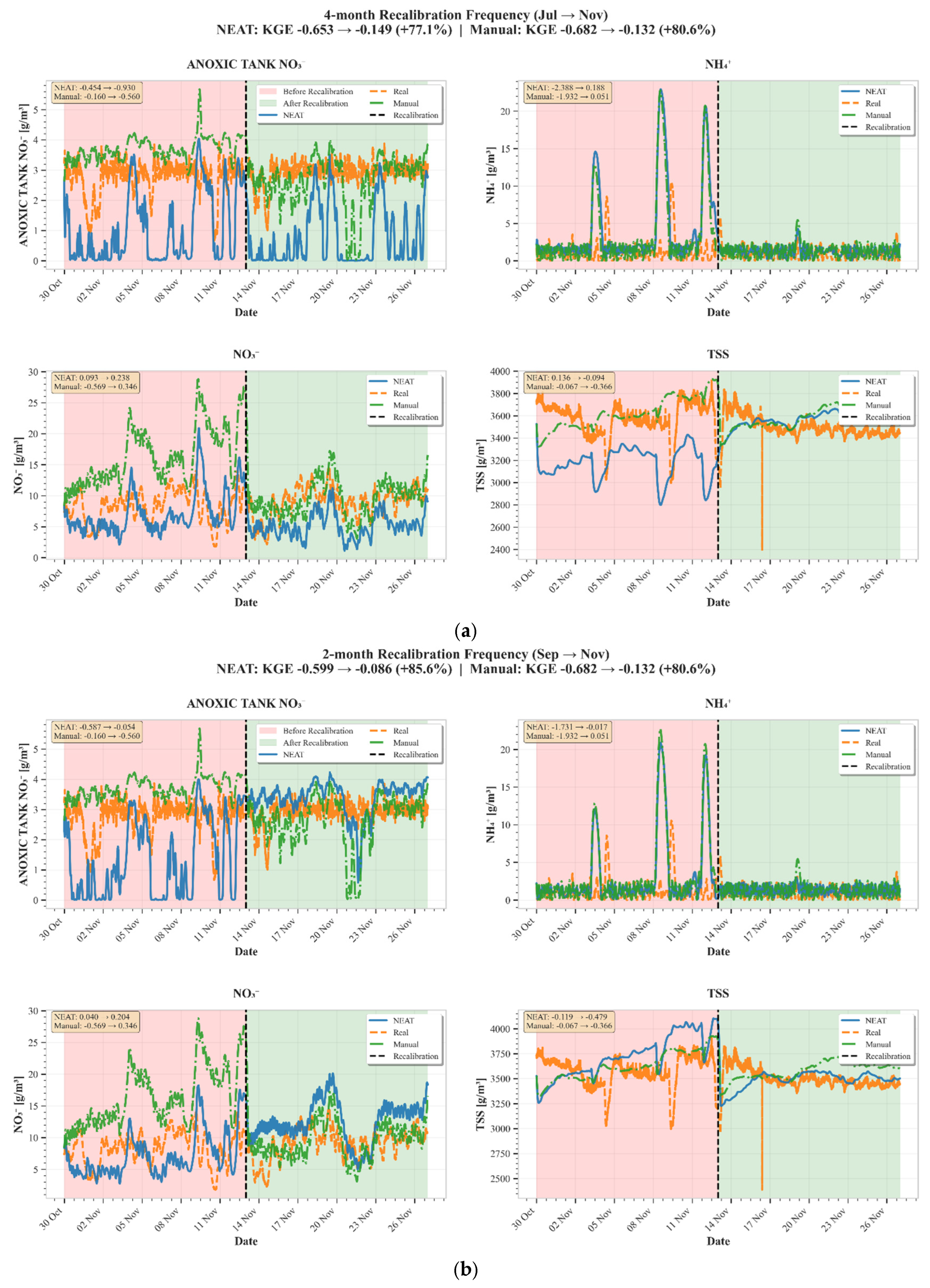
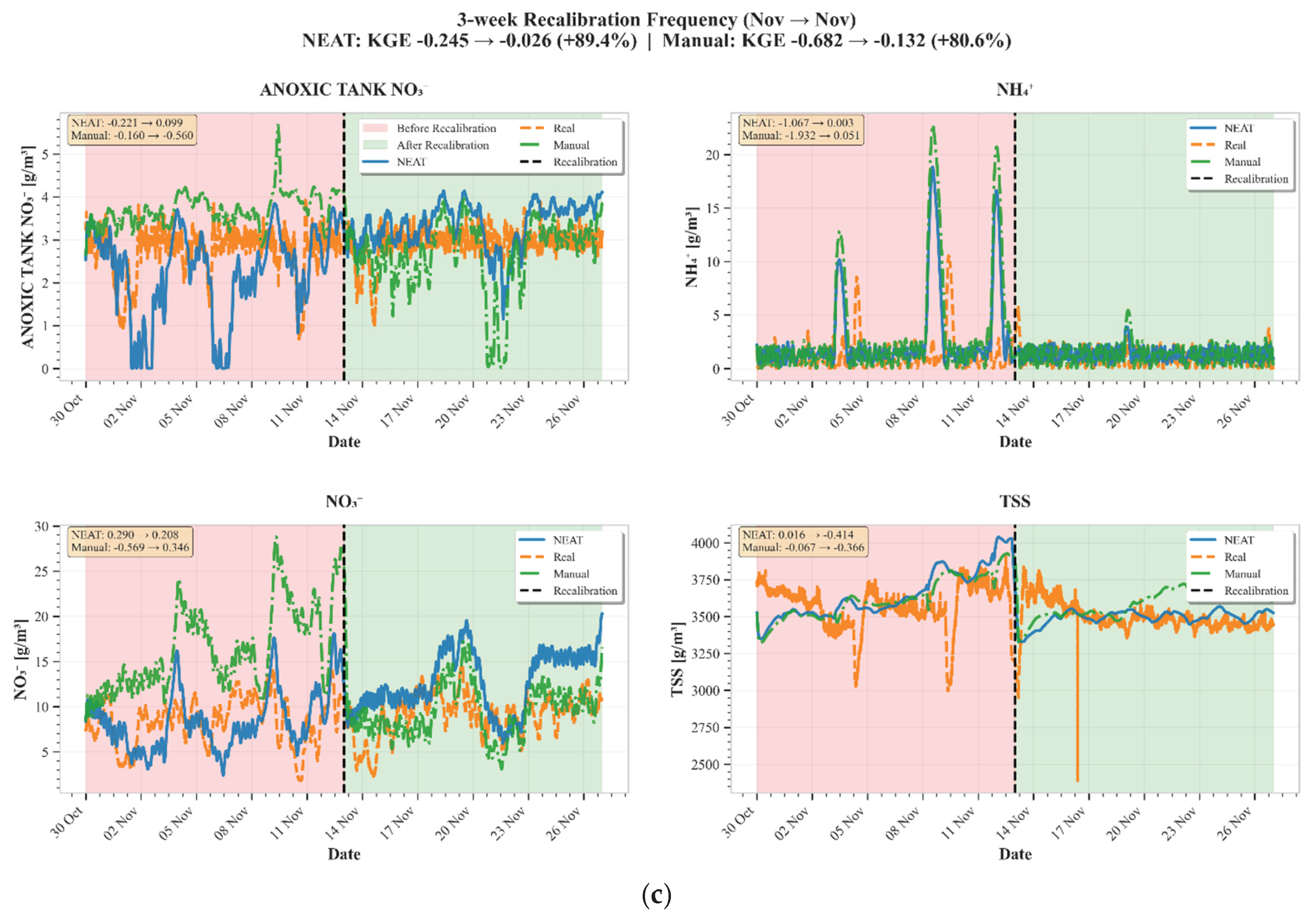
Appendix H. Secondary Metrics
In addition to KGE, two complementary metrics were calculated for validation and comprehensive performance reporting:
Root Mean Squared Error (RMSE): Quantifies the average magnitude of prediction errors, calculated as:
where yi represents observed values, ŷi represents simulated values, and n is the number of observations. RMSE was calculated for each target variable independently, and the final reported RMSE represented the average across all variables.
Coefficient of Determination (R2): Measures the proportion of variance in observed data explained by the model, calculated as:
where ȳ is the mean of observed values. Similar to KGE and RMSE, R2 was computed for each target variable, with the final metric representing the average across all variables.
References
- Amerlinck, Y. (2015). Model refinements in view of wastewater treatment plant optimization: Improving the balance in sub-model detail. http://hdl.handle.net/1854/LU-6952234.
- Benedetti, L.; Batstone, D.J.; De Baets, B.; Nopens, I.; Vanrolleghem, P.A. Global sensitivity analysis of biochemical, design and operational parameters of the Benchmark Simulation Model no. 2. In Proceedings of the iEMSs2008: International Congress on Environmental Modelling and Software, Barcelona, Spain, 7–10 July 2008. [Google Scholar]
- Borzooei, S.; Daneshgar, S.; Torfs, E.; Rehman, U.; Duchi, S.; Peeters, R.; Weijers, S.; Nopens, I. Next-Generation Compartmental Models for Applications in Digital Twinning of WRRFs. In Proceedings of the 8th IWA Water Resource Recovery Modelling Seminar, Stellenbosch, South Africa, 18–22 January 2023. [Google Scholar] [CrossRef]
- Bürger, R.; Diehl, S.; Nopens, I. A consistent modelling methodology for secondary settling tanks in wastewater treatment. Water Res. 2011, 45, 2247–2260. [Google Scholar] [CrossRef] [PubMed]
- Chen, J.; N’Doye, I.; Myshkevych, Y.; Alouini, M.-S.; Hong, P.-Y.; Laleg-Kirati, T.-M. Viral particle prediction in wastewater treatment plants using nonlinear lifelong learning models. npj Clean Water 2025, 8, 28. [Google Scholar] [CrossRef]
- Cierkens, K.; Nopens, I.; De Keyser, W.; Van Hulle, S.; Plano, S.; Torfs, E.; Amerlinck, Y.; Benedetti, L.; van Nieuwenhuijzen, A.; Weijers, S.; et al. Integrated model-based zoptimization at the WWTP of Eindhoven. Water Pract. Technol. 2012, 7, wpt2012035. [Google Scholar] [CrossRef]
- Corominas, L.; Garrido-Baserba, M.; Villez, K.; Olsson, G.; Cortés, U.; Poch, M. Transforming data into knowledge for improved wastewater treatment operation: A critical review of techniques. Environ. Model. Softw. 2018, 106, 89–103. [Google Scholar] [CrossRef]
- Daneshgar, S.; Polesel, F.; Borzooei, S.; Sørensen, H.R.; Peeters, R.; Weijers, S.; Nopens, I.; Torfs, E. A full--scale operational digital twin for a water resource recovery facility—A case study of Eindhoven Water Resource Recovery Facility. Water Environ. Res. 2024, 96, 11016. [Google Scholar] [CrossRef]
- De Mulder, C. Tying up Loose Ends: Optimization of Data Treatment and Hydrodynamic Model Structure of the Eindhoven Wastewater Treatment Plant Model. Ph.D. Dissertation, Faculty of Bioscience Engineering, Ghent University, Ghent, Belgium, 2019. [Google Scholar]
- De Mulder, C.; Flameling, T.; Weijers, S.; Amerlinck, Y.; Nopens, I. An open software package for data reconciliation and gap filling in preparation of water and resource recovery facility modeling. Environ. Model. Softw. 2018, 107, 186–198. [Google Scholar] [CrossRef]
- DHI. WEST: Modelling Biological Wastewater Treatment; DHI Group: Des Moines, IA, USA, 2022. [Google Scholar]
- Duarte, M.S.; Martins, G.; Oliveira, P.; Fernandes, B.; Ferreira, E.C.; Alves, M.M.; Lopes, F.; Pereira, M.A.; Novais, P. A review of computational modeling in Wastewater Treatment Processes. ACS EST Water 2023, 4, 784–804. [Google Scholar] [CrossRef]
- EnviroSim Associates Ltd. User Manual for BioWin 3.0; EnviroSim Associates Ltd.: Hamilton, ON, Canada, 2008. [Google Scholar]
- Esmaeili, H.; Afshar Kazemi, M.A.; Radfar, R.; Pilevari, N. From chaotic errors to natural curves: Real-coded genetic calibration of Wastewater Treatment Systems. Int. J. Environ. Sci. Technol. 2025, 22, 13557–13570. [Google Scholar] [CrossRef]
- Gomez, C.; Solon, K.; Haest, P.-J.; Morley, M.; Nopens, I.; Torfs, E. Enhancing accuracy and efficiency in calibration of drinking water distribution networks through evolutionary artificial neural networks and expert systems. J. Hydroinformatics 2025, 27, 1554–1578. [Google Scholar] [CrossRef]
- Gupta, H.V.; Kling, H.; Yilmaz, K.K.; Martinez, G.F. Decomposition of the mean squared error and NSE performance criteria: Implications for improving hydrological modelling. Journal of Hydrology 2009, 377, 80–91. [Google Scholar] [CrossRef]
- Hansen, B.D.; Hansen, T.B.; Moeslund, T.B.; Jensen, D.G. Data-driven drift detection in real process tanks: Bridging the gap between academia and Practice. Water 2022, 14, 926. [Google Scholar] [CrossRef]
- Henze, M.; Gujer, W.; Mino, T.; van Loosedrecht, M. Activated sludge models ASM1, ASM2, ASM2d and ASM3. Water Intell. Online 2006, 5, 9781780402369. [Google Scholar] [CrossRef]
- Hulsbeek, J.J.W.; Kruit, J.; Roeleveld, P.J.; van Loosdrecht, M.C.M. A practical protocol for dynamic modelling of Activated Sludge Systems. Water Sci. Technol. 2002, 45, 127–136. [Google Scholar] [CrossRef]
- Hydromantis Environmental Software Solutions Inc. GPS-X Technical Reference; Hydromantis Environmental Software Solutions Inc.: Hamilton, ON, Canada, 2017. [Google Scholar]
- Kaisler, S. Expert systems: An overview. IEEE J. Ocean. Eng. 1986, 11, 442–448. [Google Scholar] [CrossRef]
- Koksal, E.S.; Aydin, E. A hybrid approach of transfer learning and physics-informed modelling: Improving dissolved oxygen concentration prediction in an industrial wastewater treatment plant. Chem. Eng. Sci. 2025, 304, 121088. [Google Scholar] [CrossRef]
- Lumley, D.J.; Polesel, F.; Refstrup Sørensen, H.; Gustafsson, L.-G. Connecting Digital Twins to control collections systems and water resource recovery facilities: From Siloed to integrated urban (waste)water management. Water Pract. Amp; Technol. 2024, 19, 2267–2278. [Google Scholar] [CrossRef]
- Martins, A.C.; Silva, M.C.; Benetti, A.D. Evaluation and optimization of ASM1 parameters using large-scale WWTP monitoring data from a subtropical climate region in Brazil. Water Pract. Technol. 2021, 17, 268–284. [Google Scholar] [CrossRef]
- Melcer, H.; Dold, P.L.; Jones, R.M.; Bye, C.M.; Takács, I.; Stensel, H.D.; Wilson, A.W.; Sun, P.; Bury, S. Methods for Wastewater Characterization in Activated Sludge Modeling (WERF Project 99-WWF-3); Water Environment Research Foundation: Alexandria, VA, USA, 2003. [Google Scholar]
- Miranda, L.J.V. PySwarms: A research toolkit for Particle Swarm Optimization in Python. J. Open Source Softw. 2018, 3, 433. [Google Scholar] [CrossRef]
- Mnih, V.; Kavukcuoglu, K.; Silver, D.; Graves, A.; Antonoglou, I.; Wierstra, D.; Riedmiller, M. Playing Atari with deep reinforcement learning. arXiv 2013, arXiv:1312.5602. [Google Scholar] [CrossRef]
- Mustajab, A.H.; Lyu, H.; Rizvi, Z.; Wuttke, F. Physics-informed neural networks for high-frequency and multi-scale problems using transfer learning. Appl. Sci. 2024, 14, 3204. [Google Scholar] [CrossRef]
- Peirovi Minaee, R.; Afsharnia, M.; Moghaddam, A.; Ebrahimi, A.A.; Askarishahi, M.; Mokhtari, M. Calibration of water quality model for distribution networks using genetic algorithm, particle swarm optimization, and hybrid methods. MethodsX 2019, 6, 540–548. [Google Scholar] [CrossRef]
- Petersen, B.; Gernaey, K.; Devisscher, M.; Dochain, D.; Vanrolleghem, P.A. A simplified method to assess structurally identifiable parameters in monod-based activated sludge models. Water Res. 2003, 37, 2893–2904. [Google Scholar] [CrossRef] [PubMed]
- Pisa, I.; Morell, A.; Vilanova, R.; Vicario, J.L. Transfer learning in Wastewater Treatment Plant Control Design: From conventional to long short-term memory-based controllers. Sensors 2021, 21, 6315. [Google Scholar] [CrossRef]
- Prantikos, K.; Chatzidakis, S.; Tsoukalas, L.H.; Heifetz, A. Physics-informed neural network with transfer learning (TL-PINN) based on domain similarity measure for prediction of nuclear reactor transients. Sci. Rep. 2023, 13, 16840. [Google Scholar] [CrossRef]
- Protoulis, T.; Kalogeropoulos, I.; Kordatos, I.; Sarimveis, H.; Alexandridis, A. A machine learning dynamic modelling scheme for wastewater treatment plants using cooperative particle swarm optimization and neural networks. Comput. Aid. Chem. Eng. 2023, 52, 1789–1794. [Google Scholar] [CrossRef]
- Rashid, M.M.; Mhaskar, P.; Swartz, C.L.E. Optimizing wastewater treatment through artificial intelligence: Recent advances and future prospects. Water Sci. Technol. 2024, 90, 1067–1091. [Google Scholar] [CrossRef]
- Rehman, U. (2016). Next generation bioreactor models for wastewater treatment systems by means of detailed combined modelling of mixing and biokinetics. http://hdl.handle.net/1854/LU-8109100.
- Rieger, L.; Gillot, S.; Langergraber, G.; Ohtsuki, T.; Shaw, A.; Takacs, I.; Winkler, S. Guidelines for Using Activated Sludge Models; IWA Publishing: London, UK. [CrossRef]
- Rodríguez-Alonso, C.; Pena-Regueiro, I.; García, Ó. Digital Twin Platform for water treatment plants using microservices architecture. Sensors 2024, 24, 1568. [Google Scholar] [CrossRef] [PubMed]
- Ruela, I.C.S.; Carvalho, T.M.N.; Alves, R.; Rocha, G.H.O.; Rocher, V.; Poch, M.; Sin, G. A review of computational modeling in wastewater treatment processes. ACS EST Water 2023, 3, 908–931. [Google Scholar] [CrossRef]
- Samuelsson, O.; Lindblom, E.U.; Björk, A.; Carlsson, B. To calibrate or not to calibrate, that is the question. Water Res. 2023, 229, 119338. [Google Scholar] [CrossRef]
- Sin, G.; Al, R. Activated sludge models at the crossroad of Artificial Intelligence—A perspective on advancing process modeling. npj Clean Water 2021, 4, 16. [Google Scholar] [CrossRef]
- Sin, G.; Gernaey, K.V.; Lantz, A.E. Good modeling practice for pat applications: Propagation of input uncertainty and sensitivity analysis. Biotechnol. Prog. 2009, 25, 1043–1053. [Google Scholar] [CrossRef]
- Sin, G.; De Pauw, D.J.W.; Weijers, S.; Vanrolleghem, P.A. An efficient approach to automate the manual trial and error calibration of activated sludge models. Biotechnol. Bioeng. 2007, 100, 516–528. [Google Scholar] [CrossRef]
- Sin, G.; Vanhulle, S.; Depauw, D.; Vangriensven, A.; Vanrolleghem, P. A critical comparison of systematic calibration protocols for Activated Sludge Models: A SWOT analysis. Water Res. 2005, 39, 2459–2474. [Google Scholar] [CrossRef] [PubMed]
- Stanley, K.O.; Miikkulainen, R. Evolving neural networks through augmenting topologies. Evol. Comput. 2002, 10, 99–127. [Google Scholar] [CrossRef] [PubMed]
- Stentoft, P.A.; Munk-Nielsen, T.; Møller, J.K.; Madsen, H.; Valverde-Pérez, B.; Mikkelsen, P.S.; Vezzaro, L. Prioritize effluent quality, operational costs or global warming?—Using predictive control of wastewater aeration for flexible management of objectives in WRRFs. Water Res. 2021, 196, 116960. [Google Scholar] [CrossRef] [PubMed]
- Tay, J.-H. Development of a settling model for primary settling tanks. Water Res. 1982, 16, 1413–1417. [Google Scholar] [CrossRef]
- Torfs, E.; Nicolaï, N.; Daneshgar, S.; Copp, J.B.; Haimi, H.; Ikumi, D.; Johnson, B.; Plosz, B.B.; Snowling, S.; Townley, L.R.; et al. The transition of WRRF models to Digital Twin Applications. Water Sci. Technol. 2022, 85, 2840–2853. [Google Scholar] [CrossRef]
- Vanrolleghem, P.A.; Insel, G.; Petersen, B.; Sin, G.; De Pauw, D.; Nopens, I.; Dovermann, H.; Weijers, S.; Gernaey, K. A Comprehensive Model Calibration Procedure for Activated Sludge Models. In Proceedings of the 76th Annual Conference of the Water Environment Federation, Los Angeles, CA, USA, 11–15 October 2003. [Google Scholar]
- Xie, F.; Tian, C.; Ma, X.; Ji, L.; Zhao, B.; Danish, M.E.; Gao, F.; Yang, Z. Seasonal temperature effects on EPS composition and sludge settling performance in full-scale wastewater treatment plant: Mechanisms and mitigation strategies. Fermentation 2025, 11, 532. [Google Scholar] [CrossRef]
- Ye, G.; Wan, J.; Deng, Z.; Wang, Y.; Chen, J.; Zhu, B.; Ji, S. Prediction of effluent total nitrogen and energy consumption in wastewater treatment plants: Bayesian Optimization Machine Learning Methods. Bioresour. Technol. 2024, 395, 130361. [Google Scholar] [CrossRef] [PubMed]
- Yu, H.; Wang, Y.; Li, T.; Gan, Q.; Qu, D.; Qu, F. Calibrating activated sludge models through hyperparameter optimization: A new framework for Wastewater Treatment Plant Simulation. npj Clean Water 2025, 8, 80. [Google Scholar] [CrossRef]
- Zheng, Y.; Zhang, X.; Zhou, Y.; Zhang, Y.; Zhang, T.; Farmani, R. Deep representation learning enables cross-basin water quality prediction under data-scarce conditions. npj Clean Water 2025, 8, 33. [Google Scholar] [CrossRef]
- Zhou, M.; Mei, G. Transfer learning-based coupling of smoothed finite element method and physics-informed neural network for solving elastoplastic inverse problems. Mathematics 2023, 11, 2529. [Google Scholar] [CrossRef]
- Zhu, A.; Guo, J.; Ni, B.-J.; Wang, S.; Yang, Q.; Peng, Y. A novel protocol for model calibration in biological wastewater treatment. Sci. Rep. 2015, 5, 8493. [Google Scholar] [CrossRef] [PubMed]
Figure 1.
Schematic representation of the Eindhoven WRRF layout (Daneshgar et al., 2024).
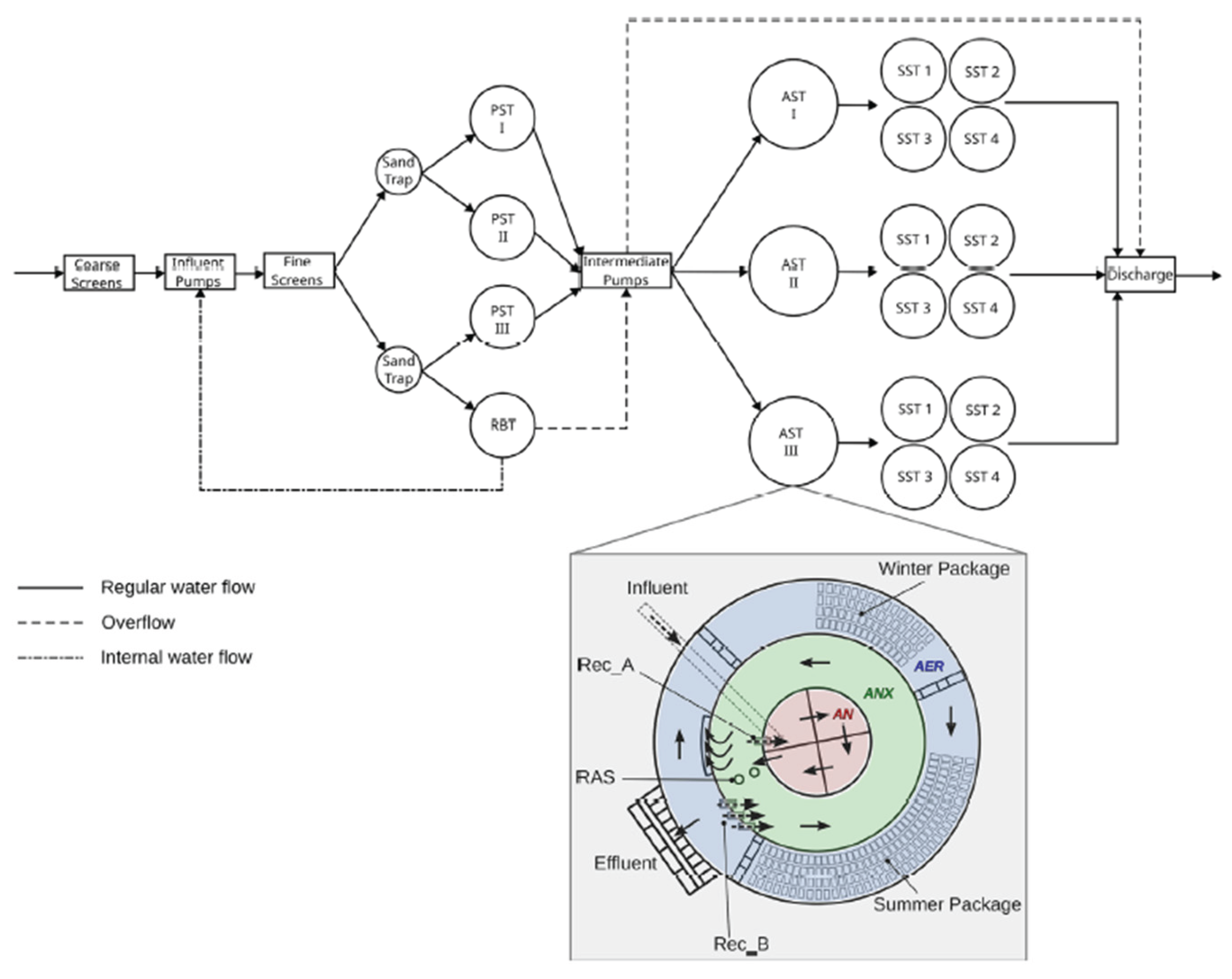
Figure 2.
Influent flow and concentrations for July, September, and November 2013 scenarios were used as calibration and validation datasets.
Figure 2.
Influent flow and concentrations for July, September, and November 2013 scenarios were used as calibration and validation datasets.
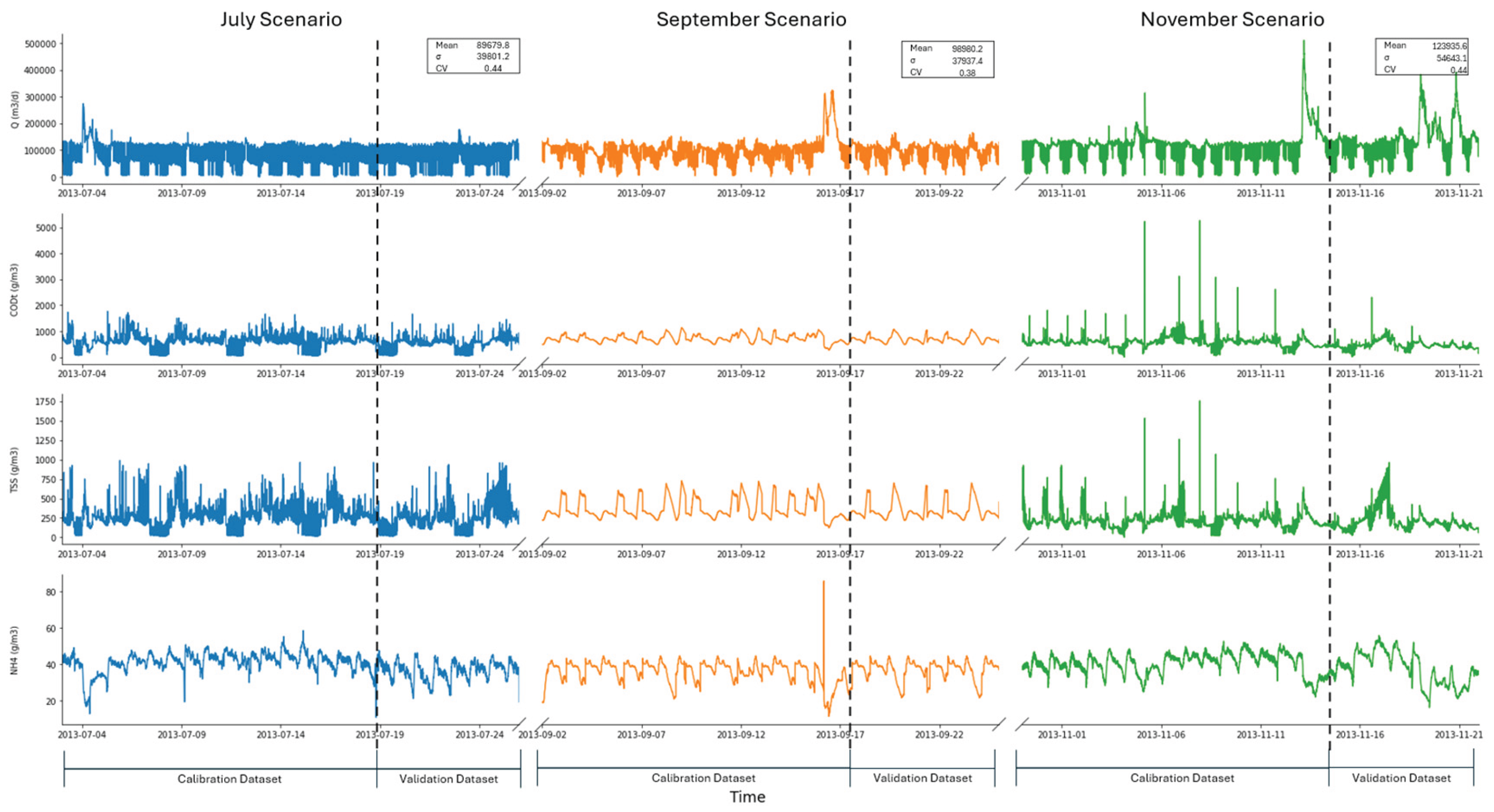
Figure 3.
Conceptual scheme of the ES-NEAT recalibration methodology.
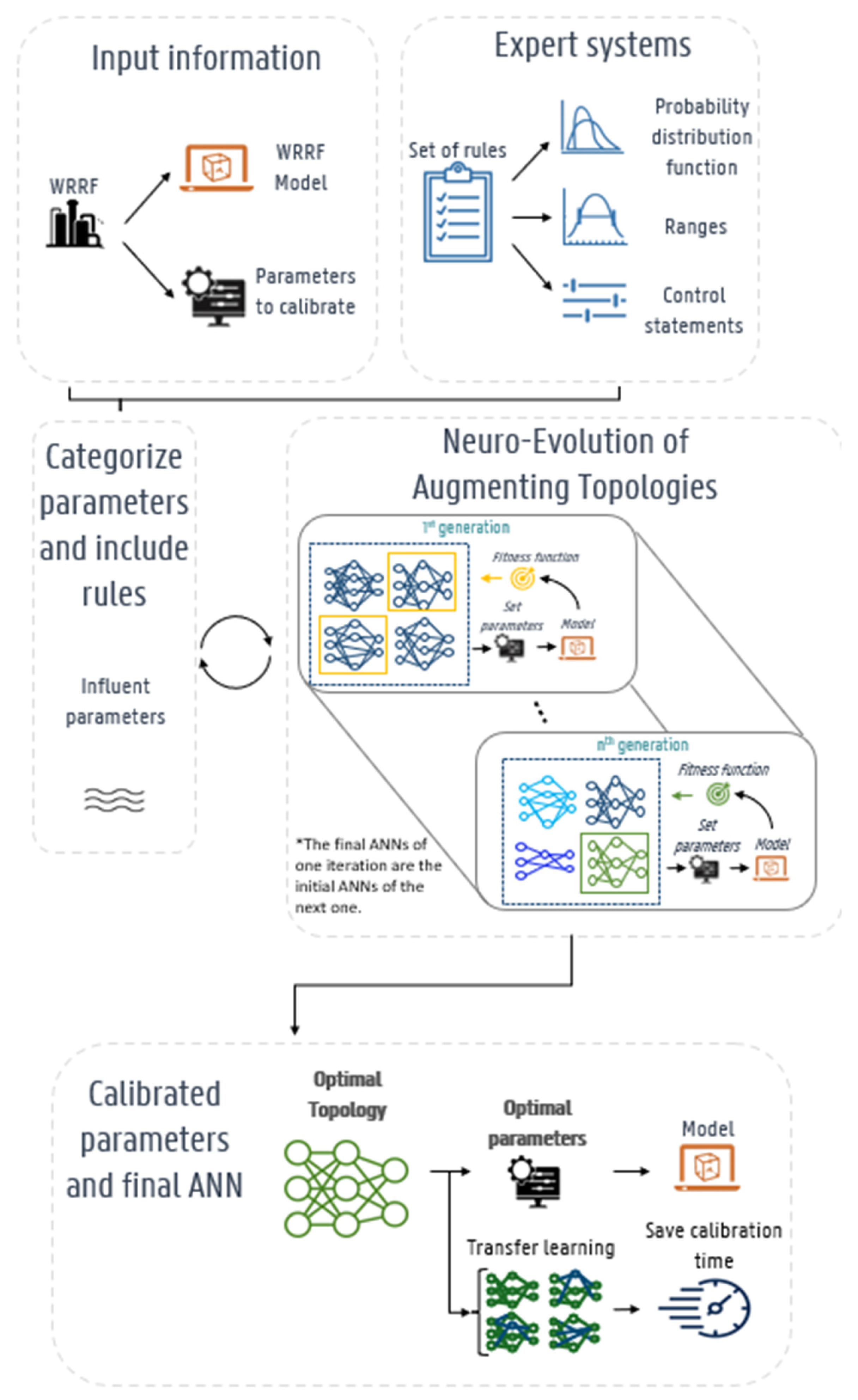
Figure 4.
Time-series comparisons between observed and simulated effluent concentrations for TSS, NH4+, and NO3− in the aerobic tank and NO3− in the anoxic tank during July 2013 calibration and validation periods (CM model only).
Figure 4.
Time-series comparisons between observed and simulated effluent concentrations for TSS, NH4+, and NO3− in the aerobic tank and NO3− in the anoxic tank during July 2013 calibration and validation periods (CM model only).
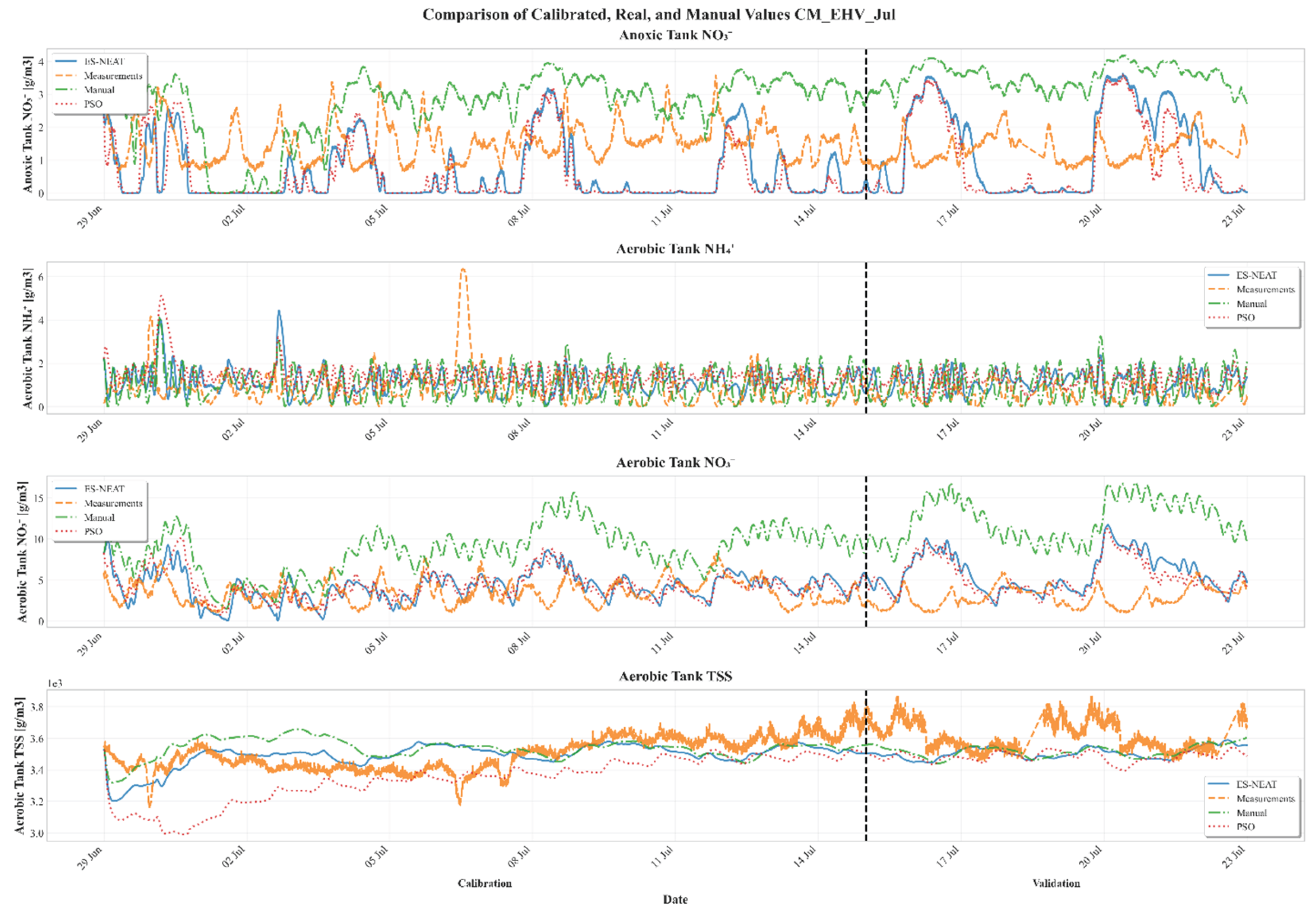
Figure 5.
Time-series comparisons of Aerobic Tank TSS for different recalibration frequencies (4-month, 2-month, 3-week intervals) during October 30–November 29 evaluation (CM model only). Shaded regions indicate degradation before recalibration and recovery post-recalibration.
Figure 5.
Time-series comparisons of Aerobic Tank TSS for different recalibration frequencies (4-month, 2-month, 3-week intervals) during October 30–November 29 evaluation (CM model only). Shaded regions indicate degradation before recalibration and recovery post-recalibration.
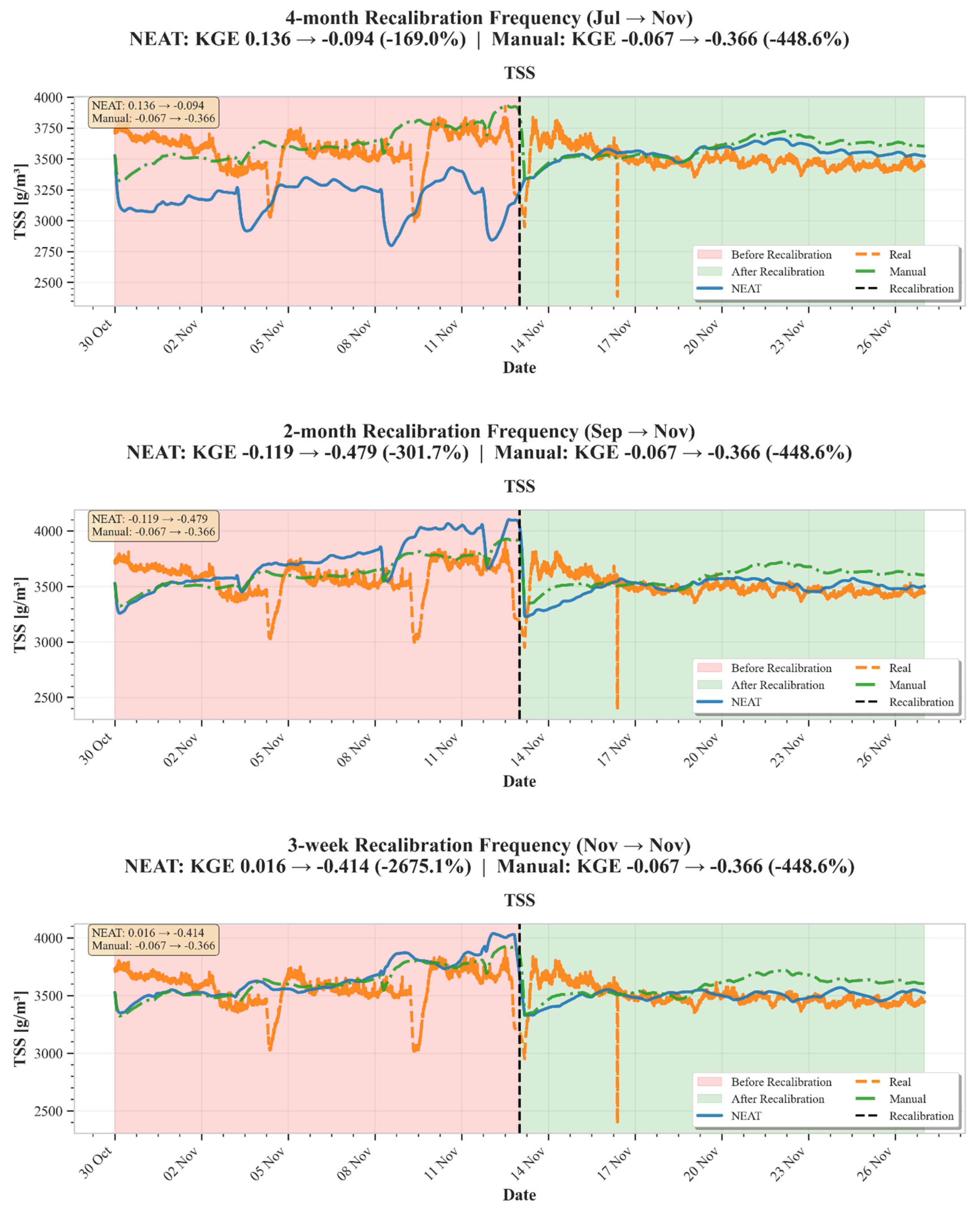
Table 1.
Calibration parameters implemented in the analysis of the Eindhoven WRRF model.
| Parameter | Symbol | Group | Default value | Bottom Limit | Upper Limit |
| Nitrogen content of biomass X_H, X_PAO, X_AUT | i_N_BM | Composition parameters | 0.07 | 0.05 | 0.09 |
| Nitrogen content of soluble substrate S_F | i_N_S_F | Composition parameters | 0.03 | 0.015 | 0.05 |
| Nitrogen content of inert soluble COD S_I | i_N_S_I | Composition parameters | 0.01 | 0.005 | 0.04 |
| Nitrogen content of inert particulate COD X_I | i_N_X_I | Composition parameters | 0.02 | 0.01 | 0.04 |
| Nitrogen content of particulate substrate X_S | i_N_X_S | Composition parameters | 0.04 | 0.02 | 0.06 |
| TSS to biomass ratio for X_H, X_PAO, X_AUT | i_TSS_BM | Composition parameters | 0.9 | 0.7 | 1 |
| TSS to X_I ratio | i_TSS_X_I | Composition parameters | 0.75 | 0.65 | 0.9 |
| TSS to X_S ratio | i_TSS_X_S | Composition parameters | 0.75 | 0.65 | 0.9 |
| Saturation/inhibition coefficient for growth on S_F | K_F | Kinetic | 4 | 1 | 8 |
| Saturation coefficient for ammonium (nutrient) | K_NH | Kinetic | 0.05 | 0.01 | 0.1 |
| Saturation coefficient of autotrophs for ammonium | K_NH_AUT | Kinetic | 1 | 0.05 | 1.2 |
| Saturation/inhibition coefficient for nitrate | K_NO | Kinetic | 0.5 | 0.1 | 0.8 |
| Saturation/inhibition coefficient for oxygen | K_O | Kinetic | 0.2 | 0.05 | 0.4 |
| Saturation/inhibition coefficient of autotrophs for oxygen | K_O_AUT | Kinetic | 0.5 | 0.2 | 1 |
| Saturation coefficient for particulate COD | K_X | Kinetic | 0.1 | 0.03 | 0.2 |
| Saturation coefficient for fermentation on S_F | K_fe | Kinetic | 4 | 2 | 6 |
| Decay rate for autotrophic biomass | b_AUT | Kinetic | 0.15 | 0.05 | 0.5 |
| Decay rate for heterotrophic biomass | b_H | Kinetic | 0.4 | 0.1 | 0.8 |
| Maximum hydrolysis rate | k_h | Kinetic | 3 | 1 | 8 |
| Maximum growth rate | mu_AUT | Kinetic | 1 | 0.5 | 1.4 |
| Maximum growth rate on substrate | mu_H | Kinetic | 6 | 3 | 12 |
| Yield For Autotrophic Biomass | Y_AUT | Stoichiometry | 0.24 | 0.15 | 0.35 |
| Yield For Heterotrophic Biomass | Y_H | Stoichiometry | 0.625 | 0.4 | 0.75 |
| Removal efficiency for particulate COD at dry weather flows | PST.E_R_XCOD_DW | Primary settler | 0.51 | 0.6 | 1 |
| Removal efficiency for inert inorganic particulates at dry weather flows | PST.E_R_XII_DW | Primary settler | 0.85 | 0.3 | 0.7 |
| Fraction of fermentation products (S_A) in the soluble COD | in.f_S_A | Influent fractionation | 0.38 | 0.25 | 0.5 |
| Fraction of fermentable readily biodegradable products (S_F) in the soluble COD | in.f_S_F | Influent fractionation | 0.39 | 0.25 | 0.4 |
| Fraction slowly biodegradable substrate (X_S) in the particulate COD | in.f_X_S | Influent fractionation | 0.43 | 0.35 | 0.7 |
| VSS to TSS ratio | in.F_VSS_TSS | Influent fractionation | 0.74 | 0.6 | 0.85 |
| Non-settleable fraction of suspended solids | SST.f_ns | Secondary settler | 0.00023 | 0.0005 | 0.003 |
| Settling parameter (hindered settling) | SST.r_H | Secondary settler | 0.00058 | 0.0002 | 0.0012 |
| Settling parameter (low concentration) | SST.r_P | Secondary settler | 0.00286 | 0.0008 | 0.009 |
| Maximum theoretical settling velocity | SST.v0 | Secondary settler | 474 | 250 | 700 |
Table 2.
Experimental design structure for recalibration analysis.
| Variable | # Components | Description |
| Model Structure | 2 | Tank-in-Series (TIS) and Compartmental Model (CM) |
| Temporal Scenario | 3 | July 2013, September 2013, November 2013 |
| Calibration Method | Varies by scenario | July: ES-NEAT, PSO, Original calibration; September & November: ES-NEAT, Original calibration |
| Target Variable | 4 | Anoxic zone NO3−, End of aeration zone NH4+, End of aeration zone NO3−, End of aeration zone TSS |
| Temporal Period | 3 per scenario | Days 1-8, Days 9-16, Days 17-24 of each 24-day calibration scenario |
| Performance Metric | 3 | KGE, R2, RMSE |
Table 3.
Comparative calibration and validation performance (KGE, R2, RMSE) and computational efficiency (iterations, computation time) for different calibration methods across scenarios and model structures.
Table 3.
Comparative calibration and validation performance (KGE, R2, RMSE) and computational efficiency (iterations, computation time) for different calibration methods across scenarios and model structures.
| Manual calibration | Calculated | Jul TIS | Jul CM | Sep TIS | Sep CM | Nov TIS | Nov CM | |
| KGE | Calibration | -0.836 | -0.333 | -0.204 | 0.110 | -1.162 | 0.099 | |
| Validation | -2.627 | -0.981 | -0.706 | -0.545 | -1.295 | -0.492 | ||
| Total | -1.732 | -0.657 | -0.455 | -0.217 | -1.229 | -0.196 | ||
| R2 | Calibration | 0.014 | 0.003 | 0.043 | 0.142 | 0.042 | 0.188 | |
| Validation | 0.052 | 0.019 | 0.064 | 0.059 | 0.124 | 0.252 | ||
| Total | 0.033 | 0.011 | 0.054 | 0.100 | 0.083 | 0.220 | ||
| RMSE | Calibration | 33.945 | 33.725 | 103.937 | 111.383 | 46.419 | 47.340 | |
| Validation | 39.213 | 36.843 | 68.773 | 95.577 | 44.509 | 71.036 | ||
| Total | 36.579 | 35.284 | 86.355 | 103.480 | 45.464 | 59.188 | ||
| PSO calibration | Calculated | Jul TIS | Jul CM | Sep TIS | Sep CM | Nov TIS | Nov CM | |
| KGE | Calibration | -0.125 | 0.017 | 0.065 | -0.069 | -0.109 | 0.240 | |
| Validation | -0.877 | -0.562 | -0.107 | -0.069 | -0.312 | -0.356 | ||
| Total | -0.501 | -0.272 | -0.021 | -0.069 | -0.210 | -0.058 | ||
| R2 | Calibration | 0.004 | 0.085 | 0.148 | 0.050 | 0.260 | 0.225 | |
| Validation | 0.073 | 0.091 | 0.092 | 0.052 | 0.280 | 0.305 | ||
| Total | 0.039 | 0.088 | 0.120 | 0.051 | 0.270 | 0.265 | ||
| RMSE | Calibration | 28.413 | 51.685 | 93.150 | 96.439 | 34.313 | 39.945 | |
| Validation | 38.162 | 40.254 | 45.868 | 58.825 | 40.019 | 49.770 | ||
| Total | 33.287 | 45.969 | 69.509 | 77.632 | 37.166 | 44.858 | ||
| Computational Time (hours) | 10 | 12 | 3 | 4 | 5 | 6 | ||
| Number of generations | 100 | 100 | 11 | 14 | 19 | 24 | ||
| PSO calibration | Calculated | Jul CM | Sep CM | |||||
| KGE | Calibration | 0.037 | -0.040 | |||||
| Validation | -0.671 | -0.197 | ||||||
| Total | -0.317 | -0.118 | ||||||
| R2 | Calibration | 0.033 | 0.040 | |||||
| Validation | 0.049 | 0.074 | ||||||
| Total | 0.041 | 0.057 | ||||||
| RMSE | Calibration | 28.723 | 62.217 | |||||
| Validation | 38.123 | 51.031 | ||||||
| Total | 33.423 | 56.624 | ||||||
| Computational Time (hours) | 12 | 12 | ||||||
| Number of generations | 100 | 100 | ||||||
Disclaimer/Publisher’s Note: The statements, opinions and data contained in all publications are solely those of the individual author(s) and contributor(s) and not of MDPI and/or the editor(s). MDPI and/or the editor(s) disclaim responsibility for any injury to people or property resulting from any ideas, methods, instructions or products referred to in the content. |
© 2025 by the authors. Licensee MDPI, Basel, Switzerland. This article is an open access article distributed under the terms and conditions of the Creative Commons Attribution (CC BY) license (http://creativecommons.org/licenses/by/4.0/).
Copyright: This open access article is published under a Creative Commons CC BY 4.0 license, which permit the free download, distribution, and reuse, provided that the author and preprint are cited in any reuse.