Submitted:
07 November 2025
Posted:
10 November 2025
You are already at the latest version
Abstract
Subsea drilling rig main shaft bearings are among the critical rotating components of the rig, and their health status directly affects the efficiency and reliability of the drilling system. However, in the deep-sea high-pressure and intense-noise liquid environment, the vibration signals of the bearings attenuate rapidly, resulting in an extremely low Signal-to-Noise Ratio (SNR) for the fault features, posing a challenge to bearing health monitoring. In recent years, Deep Neural Network (DNN)- based fault diagnosis methods for subsea drilling rig bearings have become a research hotspot in the field due to their strong capability for deep fault feature mining. Nevertheless, their reliance on high-power consumption computational resources restricts their widespread application in subsea monitoring scenarios. To address the above issues, this paper proposes an innovative fault diagnosis method for subsea drilling rig bearings based on Population Coding combined with an Adaptive Threshold k-Winner-Take-All (k-WTA) mechanism. This method introduces the Adaptive Threshold k-WTA mechanism during the population coding process of the SNN’s Gaussian receptive field. This not only sparsely filters the activation values but also optimizes energy efficiency by reducing the amplitude of spike emission. This effectively utilizes the feature representation capability of Population Coding and the activation sparsity of the k-WTA mechanism to realize a high anti-noise, lower-energy-consumption fault diagnosis solution for subsea drilling rig main shaft bearings. The experimental results demonstrate that, in the accuracy and generalization experiments, the proposed method achieves high diagnostic accuracy on both the CWRU benchmark dataset and the self-collected deep-sea testbed dataset, reflecting strong generalization and robustness. The results on the real bearing Paderborn benchmark dataset highlight the importance of feature selection tailored to specific operating conditions. Additionally, in the noise robustness and energy efficiency experiments, the proposed method shows significant advantages in both noise resistance and energy efficiency.
Keywords:
subsea drilling rig
; main shaft bearings
; fault diagnosis
; spiking neural network
; k-WTA
; low power consumption
1. Introduction
With the increasing depletion of terrestrial resources worldwide, the ocean has become a vital strategic field for resource exploration and development in the 21st century [1,2]. As the core equipment for the exploitation of marine oil and gas resources, subsea drilling rigs operate long-term in extreme environments characterized by deep-sea high pressure, intense corrosion, and variable loads. This poses extremely high demands on the equipment’s safety and reliability. The Subsea Drilling Rig Main Shaft Bearings serve as critical rotating components that transmit power and receive the shock loads from drilling. Consequently, their health condition directly influences the equipment’s operational reliability and working efficiency.
Unlike land-based equipment, the operating environment for subsea drilling rig bearings is exceptionally harsh. The strong damping effect of the deep-sea liquid medium causes the vibration signals generated by bearing faults to rapidly attenuate. Concurrently, drilling operations, ocean currents, and marine biological activity all generate significant background noise. This results in the collected bearing vibration signals generally exhibiting characteristics of a low Signal-to-Noise Ratio and weak fault features.Furthermore, the scarcity of energy resources in offshore and deep-sea environments imposes stringent requirements on the power consumption of the diagnostic system. Therefore, researching a diagnostic method that can accurately and reliably identify subsea drilling rig main shaft bearing faults against a strong noise background while also ensuring low energy consumption is of practical significance for guaranteeing the safety of marine engineering equipment and improving resource extraction efficiency.
Methodologies for bearing fault diagnosis are typically bifurcated into model-driven and data-driven categories. Model-driven techniques depend heavily on detailed physical models and expert-level domain knowledge, which complicates the creation of precise models for harsh operational settings, such as deep-sea conditions. In contrast, data-driven methodologies leverage bearing fault training data to model the intricate, non-linear mapping from raw sensory input to the fault dimension, reducing the dependency on a priori knowledge. These methodologies are generally categorized into Machine Learning (ML) and Deep Learning (DL) branches. Classic ML approaches, like Principal Component Analysis (PCA) [3,4,5], Support Vector Machine (SVM) [6,7,8,9], and k-Nearest Neighbor (KNN) [10,11,12], are adept at identifying lower-level patterns from the data. Their performance, however, is contingent upon the quality of hand-crafted feature extraction. For these methods, it remains difficult to accurately characterize and differentiate weak, highly-distorted fault features, especially within the complex high-pressure, high-noise environments.
Deep Learning methods, through complex network architectures, can adaptively represent the internal correlations of the data and extract deep and robust hidden details from raw data, effectively bypassing the strong reliance of traditional methods on manual expertise. For example, Convolutional Neural Network (CNN) [13,14,15,16] excel in feature extraction, while Long Short-Term Memory network (LSTM) [17,18,19] are proficient at capturing the temporal dependencies of vibration signals. Furthermore, Autoencoders (AE) [20,21,22,23] and Deep Belief Networks (DBN) [24,25,26] are also frequently used for feature dimensionality reduction and deep learning.Although Deep Learning demonstrates excellent diagnostic accuracy, its over-reliance on high-power computing resources creates a new contradiction with the stringent condition of limited power supply for deep-sea monitoring equipment.
As the third-generation neural network, the SNN has been introduced into the field of fault diagnosis, thanks to its event-driven operational mechanism and its potential for processing complex spatiotemporal information [27,28]. SNN neurons only emit a spike when receiving sufficient stimuli. This sparse and asynchronous computational approach provides SNN with a natural ability for noise suppression and inherent low power consumption characteristics. However, the application of SNN in the fault diagnosis of marine engineering equipment, particularly in the specific scenario of subsea drilling rig bearing diagnosis, is still in its nascent stage.Therefore, this paper proposes a subsea drilling rig bearing fault diagnosis method based on Adaptive Threshold k-Winner-Take-All (k-WTA) combined with Population Coding, aiming to construct an efficient, highly robust, and low-power fault diagnosis model.
We conducted comprehensive experimental validation of the proposed method on two types of datasets: one type consists of publicly available land-based benchmark datasets (including CWRU and Paderborn University dataset), and the other consists of a self-developed deep-sea drilling platform bearing fault dataset, which simulates real-world operating conditions. In terms of diagnostic accuracy and generalization ability, the method achieves state-of-the-art (SOTA) levels of high accuracy on the CWRU benchmark, while its differentiated performance on the PU dataset emphasizes the critical importance of feature selection tailored to specific operating conditions. Regarding noise robustness, the method significantly outperforms baseline models on artificially noise-augmented datasets, and more importantly, it maintains high diagnostic accuracy on the self-collected deep-sea testbed dataset, which inherently contains strong noise and signal attenuation, demonstrating its robustness in real-world harsh environments. Finally, in terms of energy efficiency, the proposed method shows significant advantages over traditional ANN and standard SNN models across all three datasets, highlighting its potential for low-power monitoring applications in deep-sea environments.Based on the existing research, the main contributions of this paper are concentrated in the following three aspects:
- Targeted Methodological Application: This paper presents a novel application of Spiking Neural Network, specifically leveraging its low power consumption and event-driven advantages to address the unique challenges of low signal-to-noise ratio and high power consumption in underwater drilling rig bearing fault diagnosis.
- Technical Contribution: We propose a novel encoding strategy that integrates Gaussian Receptive Field-based encoding with the adaptive-threshold k-Winner-Takes-All mechanism in SNN. This innovative combination effectively optimizes energy efficiency by reducing pulse amplitude and frequency without compromising the transmission of information.
- Validation and Proof:Through extensive experiments on both publicly available benchmark datasets (CWRU and PU) and a self-developed testbed dataset, we systematically validate the performance of the proposed method across three core metrics: diagnostic accuracy, noise robustness, and energy efficiency. The experimental results demonstrate that the proposed method offers a comprehensive advantage in terms of accuracy, robustness, and power consumption, showcasing its potential for low-power monitoring applications in deep-sea environments.
Section 2 provides a detailed description of the proposed method, including signal preprocessing and feature extraction techniques tailored to the characteristics of deep-sea environments, the core spike encoding mechanism, the SNN neuron model, and the model’s training strategy. Section 3 presents the experimental study, which focuses on three core dimensions: diagnostic accuracy, noise robustness, and energy efficiency. Finally, Section 4 briefly summarizes the research findings and discusses potential directions for future work.
2. Methodology
The proposed diagnostic procedure for bearing faults is outlined in Figure 1. First, the raw vibration signal of the subsea drilling rig main shaft bearing is collected via an accelerometer sensor. Second, to extract high-quality input fault features, the Local Mean Decomposition (LMD) method is applied to the raw vibration signal, decomposing it into a linear combination of a series of Product Functions (PFs). Third, the extracted features are transformed into stable, high-information-content, and low-amplitude spike information through Gaussian Receptive Field Population Encoding combined with the Adaptive Threshold k-WTA mechanism. Subsequently, the SNN is trained using the Surrogate Gradient-based Backpropagation (BP) algorithm. Fourth, the encoded features are input into the trained SNN model to achieve the final bearing fault diagnosis. The key technical aspects are detailed in the subsequent sections.
2.1. LMD-Based Feature Extraction
The complexity of stratum drilling, rolling element skidding, and faults generating multiple shocks, all overlaid by the complex background noise of the subsea drilling rig, results in the main shaft bearing fault vibration signals having complex and overlapping frequency bands. To minimize the influence of non-linear factors and meet the subsequent requirements for stability and linearity of the input signal, preprocessing the raw vibration signal with a suitable signal processing algorithm is necessary. A variety of signal processing techniques are prevalent in the literature for bearing fault diagnosis, including established methods like Fourier Transform (FT), Wavelet Transform (WT), Empirical Mode Decomposition (EMD), and LMD. Nonetheless, these algorithms exhibit certain inadequacies when applied to the highly complex vibration signals originating from subsea main shaft bearings. To illustrate, the FT, while capable of intuitively presenting the frequency makeup of a signal, is inherently ill-suited for processing non-stationary signals. Given that subsea drilling rigs operate in complex geological strata, with continuous changes in shock, vibration, and load during the drilling process, the signals lack the required statistical properties of stationary signals.The WT possesses the characteristic of scale contraction, allowing it to analyze local features of a signal in both time and frequency, making it suitable for non-stationary signals. Nevertheless, the empirical nature of selecting the wavelet basis function and the complex computation of the Continuous Wavelet Transform limit its application in real-time scenarios.The EMD often suffers from the problem of mode mixing when dealing with pulse interference and strong noise in the vibration signals of subsea drilling rig bearings, which can render the analysis results unusable.The LMD method can decompose non-linear signals with multiple superimposed vibration modes into a series of single-component signals, each possessing an instantaneous amplitude and instantaneous frequency. These components are PFs, which can be represented in the form of an Amplitude Modulation (AM) signal multiplied by a Frequency Modulation (FM) signal. By adopting a more localized and robust decomposition strategy, LMD generally proves to be more advantageous in processing complex signals. Therefore, this paper will process the raw subsea drilling rig bearing vibration signal using LMD and extract the fault features from the resulting Product Functions. The brief implementation procedure is as follows:
- For a given signal , the first step is to identify all its local extreme points . Based on these extreme points, two numerical values are constructed: the local mean and the local envelope :where i denotes the index of the PF, j denotes the iteration number during the decomposition process and k denotes the index of the extreme value.
- Using the moving average method to generate the local mean function and the envelope function , and subtracting the local mean function from the signal , yields a detrended signal :
- Normalize the detrended signal by dividing it by the local envelope function to obtain an ideal purely Frequency-Modulated signal :
- If does not satisfy the criterion for a purely FM signal, then is taken as the new input signal, and the aforementioned Steps 1-3 are repeated until the convergence condition is met. If the iteration converges, the final purely FM signal is multiplied by the product of all local envelope functions obtained during all iteration steps. The result is the final Product Function :where l refers to the maximum number of iterations.
- Subtract the extracted from the original signal to obtain the residue signal :
- Take as the new input signal, and repeat the entire aforementioned procedure to extract the next PF component, until the final residue signal becomes a monotonic function and can no longer be decomposed. The original signal will then be decomposed as:
The components (Product Functions) generated by the LMD process remain information-dense and voluminous. Utilizing these components directly as an input feature vector would create a high-dimensional feature space, which in turn would substantially increase the computational complexity of the training algorithm. Therefore, the decomposed PF signals and the residual signal must be refined to extract the most representative and discriminative fault features of the subsea drilling rig bearings for use as input feature values.Therefore, we use the first five PF signals and one residual signal obtained from LMD decomposition as the input signals for fault feature extraction, as shown in Figure 2.
In the high-pressure fluid environment of the deep sea, the high-density damping fluid acts as damping medium, leading to the attenuation of bearing vibration energy. This high-pressure environment also alters the time-varying stiffness and modal characteristics of the system through fluid-structure interaction effects. Consequently, the selection of fault features must prioritize indicators capable of capturing the signal’s intrinsic waveform structure or periodicity, while exhibiting scale-invariance to the amplitude attenuation induced by the external environment. Specifically, this paper extracts five features from each PF component and the residual signal: Kurtosis, Crest Factor, Impulse Factor, Spectral Energy, and Spectral Kurtosis, as shown in Table 1.
The variables used in Table 1 are defined as follows: N is the total number of sampling points in the signal segment, is the discrete time-domain signal (PF component or residual), is the mean value of the time-domain signal , is the Root Mean Square (RMS) value of the time-domain signal , is the Discrete Fourier Transform (DFT) coefficient of the signal at the k-th frequency bin, is the power spectrum estimate (e.g., ) at the k-th frequency bin, is the center frequency of the k-th frequency bin, is the center frequency of the analysis band, and is the maximum absolute value (peak value) of the signal .
2.2. SNN Configuration for Subsea Diagnosis
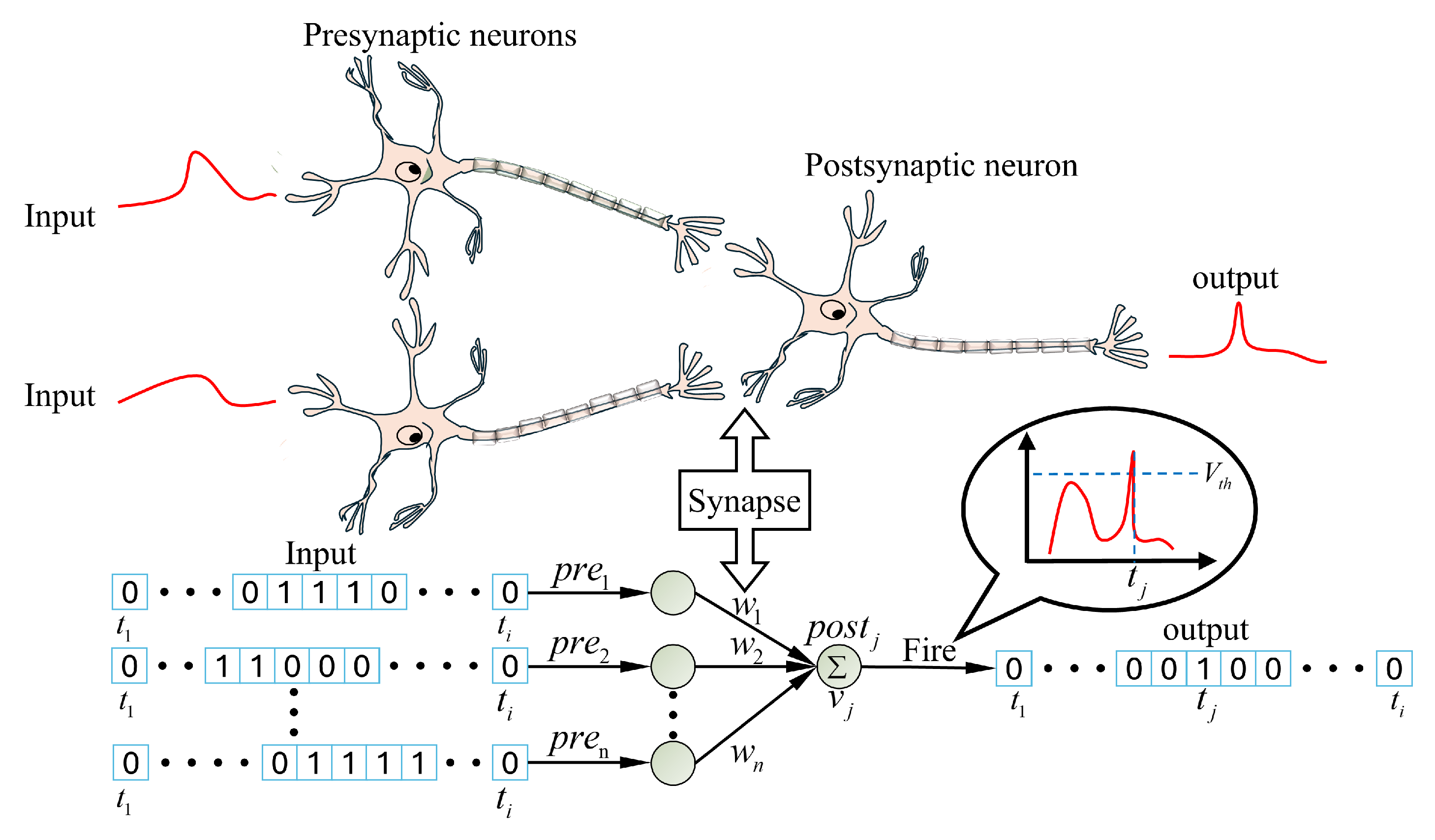
The computation of the Spiking Neural Network (SNN) is based on discrete action potentials rather than continuous values, simulating the behavior patterns of biological neurons. In the SNN, information is transmitted in the form of spikes from presynaptic neurons to postsynaptic neurons. The logical core lies in the dynamic change of the membrane potential.
When a postsynaptic neuron receives any incoming spike, its membrane potential increases accordingly. The function of this membrane potential is the continuous accumulation and integration of all received signals over time. Once the neuron’s membrane potential level reaches and surpasses a predetermined firing threshold, it immediately responds by emitting a new output spike. Immediately thereafter, the neuron’s membrane potential is reset to its resting potential state in preparation for the next round of information processing. The architectural design of the SNN and this event-driven spike generation and reset mechanism are illustrated in detail in Figure 4.
Figure 3.
Spiking neuron information transfer Process.
2.2.1. Proposed Encoding Mechanism
Unlike the continuous floating-point activation value transmission mode of Artificial Neural Network (ANN), the SNN utilizes discrete spike emissions occurring at precise time points to transmit complex information. This event-driven computational style and spike sparsity allow SNN to reduce computational activity, achieving the advantages of low power consumption and high efficiency. Therefore, for classifying subsea drilling rig bearing faults using the SNN, an appropriate encoding scheme is required to convert the aforementioned feature information into spike sequences.
Current spike encoding methods are mainly categorized into Rate Coding, Temporal Coding, and Population Coding.Rate Coding expresses information through the average spiking activity but does not rely on precise spike timing, offering strong robustness. However, it requires prolonged integration and statistics collection, leading to high latency, and the frequent spiking activity results in higher computational power consumption.Temporal Coding utilizes the precise time of spike firing to encode information. It can transmit information with the minimum number of spikes, achieving extremely low computational power consumption and ultra-low latency response speeds. Nevertheless, the limitation of Temporal Coding is its reliance on precise spike timing, making it more sensitive to noise caused by the environment or hardware, and typically requiring more complex architectures and algorithms for processing.Population Coding represents information through the coordinated activity of a group of neurons, achieving strong robustness against random noise and perturbations, as well as accurate representation of feature values. When combined with sparse representation, it can also bring about significant low-power consumption advantages.
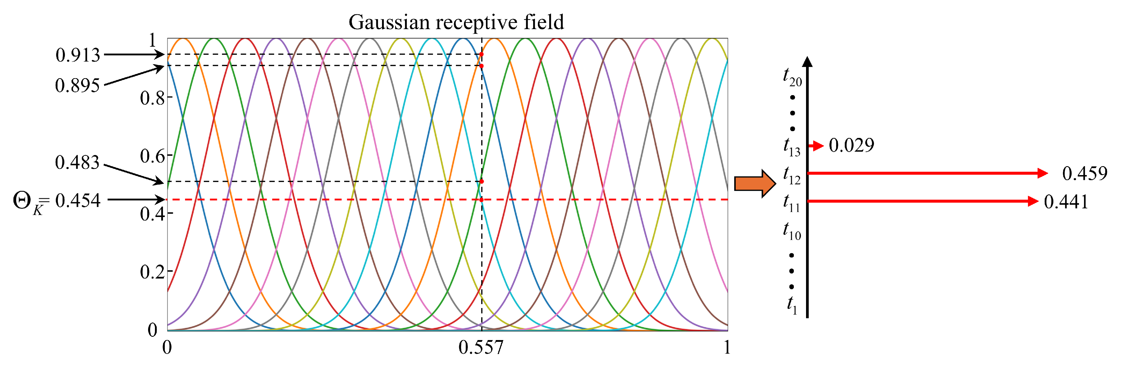
Therefore, we propose a spike encoding method based on Gaussian Receptive Fields combined with an Adaptive Threshold k-Winner-Take-All (k-WTA) mechanism. This method skillfully utilizes the feature redundancy of Population Coding and the activation sparsity of the Adaptive k-WTA mechanism to simultaneously satisfy the dual requirements of anti-noise capability and low power consumption in the deep-sea edge computing environment. The implementation steps are as follows:
First, to map features of different scales to a unified range, the entire dataset must be scaled globally, as follows:
where and are the minimum and maximum values in the extracted feature set, respectively.
Set the encoding population to consist of N neurons, where each neuron defines a unique Gaussian tuning curve T. The center position and the Gaussian receptive field width for the i-th neuron are defined as:
where is a hyperparameter .
Substitute into the receptive field defined by N Gaussian tuning curves to calculate the raw activation intensity for each neuron:
where is the maximum activation intensity, which is usually set to 1.
Perform Adaptive Threshold k-WTA screening on the activation values to retain the K neurons with the highest activation intensity in the set .
Define the K-th highest activation intensity as the adaptive threshold . The final output intensity is then derived through a comparison operation with the adaptive threshold :
The final feature F is then encoded into a spike sequence . For instance, a normalized real-valued feature of is encoded within a Gaussian receptive field consisting of neurons. Subsequently, the activation values are sparsely filtered using the Adaptive Threshold mechanism and the k-WTA competitive strategy, yielding a sparse output vector ( ). This encoding and competition process is detailed in Figure 4.
Figure 4.
Real-valued feature encoding process.
2.2.2. AdEx Neuron Model
This paper adopts the Adaptive Exponential Integrate-and-Fire (AdEx) [29] model as the neuron model for the SNN, as this model strikes a good balance between dynamical richness and computational complexity. The AdEx model functions as a hybrid dynamical system, where its behavior is collectively defined by continuous threshold dynamics and discrete spike firing events. The formula for the discrete-time update of the membrane voltage of the j-th postsynaptic AdEx neuron is defined as:
where is the leak conductance, is the resting potential, is spike sharpness, is the effective threshold potential, is the synaptic weight between the i-th presynaptic neuron and the j-th postsynaptic neuron, is the spike sequence output of the i-th presynaptic neuron and is the adaptation variable, defined as follows:
where is the time step, is the adaptation time constant, and b is a hyperparameter.
The triggering condition for the AdEx neuron’s spike firing event is when the membrane potential exceeds a set peak voltage .The instantaneous reset rules are as follows:
where is the output value of the j-th postsynaptic neuron at time step , is the resting voltage, and a is a hyperparameter.
2.2.3. Model Training Strategy
Currently, there are three main types of mainstream training algorithms for Spiking Neural Networks: the bio-inspired Spike-Timing-Dependent Plasticity (STDP) [30], the indirect ANN-SNN Conversion method [31], and the direct training approach of Surrogate Gradient Descent [32].The STDP algorithm boasts high biological plausibility but often suffers from limited diagnostic accuracy, making it difficult to satisfy the requirements of industrial scenarios. While the ANN-SNN conversion method can inherit the high accuracy of the source ANN, its drawback is that the converted SNN often requires consuming many time steps during inference to precisely approximate the source network’s performance. This dependency leads to high latency in model inference.
Given the practical demands for real-time performance and low power consumption in subsea drilling rig fault diagnosis, the Surrogate Gradient Descent method—as a direct training approach—is able to achieve high diagnostic accuracy while constructing low-latency, high-energy-efficiency diagnostic models. This makes it the optimal choice for simultaneously addressing the performance and edge deployment efficiency requirements for subsea bearing fault diagnosis.Therefore, this paper will adopt Surrogate Gradient Descent as the training method for the Spiking Neural Network. A brief introduction to the SNN training method based on Surrogate Gradient Descent is presented below.
For multiclass classification tasks like bearing fault diagnosis, the most commonly used and robust choice is the combination of Cross-Entropy Loss and Softmax. Their definitions are as follows:
where is the one-hot encoding of the true label, is the probability of class j given by the Softmax function, and is the total number of spikes emitted by the output neuron of class i.
The complete gradient formula for the hidden layer weights is expressed as:
where is the connection weight between the i-th neuron in the -th layer and the j-th neuron in the l-th layer, is the error signal of the k-th neuron in the -th layer at time step t, is the membrane voltage of the j-th neuron in the l-th layer at time step t , is the firing threshold voltage, is the spike output of the i-th neuron in the -th layer at time step t,and is the Arctangent Surrogate Gradient Function, defined by the derivative as:
In the above expression, represents the membrane potential relative to the threshold, while , the adjustable parameter controlling the gradient steepness, is set to 25.
The update formula for the connection weight is as follows:
where is the learning rate.
3. Experiment
To systematically evaluate the performance of the bearing fault diagnosis method proposed in this paper, a series of diagnostic experiments are conducted in this chapter.Given the current lack of a recognized public benchmark dataset for deep-sea operating conditions, and to ensure experimental objectivity and comparability, we introduce two public terrestrial benchmark datasets (CWRU and Paderborn) to test the model’s fundamental effectiveness and generalization capability. Secondly, to examine the model’s actual performance and practical value under the target operating conditions, this study also utilizes a bearing dataset collected from the "Subsea Drilling Rig Main Spindle Condition Simulation Test Rig," which was built by our research team, to verify the model’s true performance in the final target application scenario.
The content of this chapter is organized as follows: Section 3 introduces the datasets, Section 3.2 details the experimental design, and Section 3.3 compares and analyzes the experimental results. All experiments were conducted on a Windows 11 (64-bit) operating system. The hardware configuration was an Intel® Core™ i9-13980HX CPU with 16.0 GB of RAM, and the software environment was implemented based on Anaconda Navigator and PyCharm.
3.1. Dataset Introduction
3.1.1. CWRU Dataset
The CWRU bearing dataset, published by the university’s Bearing Data Center [33], is an internationally recognized benchmark dataset for rolling element bearing fault diagnosis.The data for this dataset was collected from a specially constructed test platform. This platform primarily consists of a 2-horsepower (HP) drive motor, a power test meter , a torque sensor, and control electronics. The experimental bearing was installed on the motor’s main shaft to support the rotor .
The CWRU dataset introduces single-point faults separately on the IR, OR, and rolling elements of the test bearings using Electro-Discharge Machining technology. Each fault location includes three different levels of damage severity, with fault diameters of 0.007 inches, 0.014 inches, and 0.021 inches, respectively.Vibration signals were acquired by accelerometers installed on the motor casings at both the drive end and the fan end. The data acquisition utilized two main sampling frequencies: 12 kHz and 48 kHz. The experiments covered four different motor load conditions, ranging from 0 to 3 horsepower, simulating the bearing’s operational status under various loads.
The CWRU dataset covers a variety of motor loads, fault locations, and fault scales. To ensure the representativeness and comparability of the experimental results, this study selected specific, typical operating conditions for model validation (detailed bearing selections are shown in Table 2).
During the sample extraction phase, all vibration signals were segmented into samples with a length of 4096 sampling points. For each fault state, 100 data samples were extracted, resulting in a total of 1000 samples, to ensure a sufficient sample size for training and testing.
3.1.2. Paderborn University Dataset
The Paderborn University dataset dataset (PU) [34], provided by Paderborn University in Germany, is another internationally recognized benchmark for bearing fault diagnosis. Unlike the artificial EDM faults in the CWRU dataset, it primarily contains real, naturally formed faults generated through accelerated life tests. The data for this set was collected from a modular test rig, as shown in Figure 5, which is capable of simulating different rotational speeds, loads, and radial force conditions.The fault types within the dataset are diverse, including pitting caused by fatigue, plastic deformation, and indentations resulting from particle contamination. Vibration signals were captured by an accelerometer mounted on the bearing housing, while the test rig also recorded operating parameters such as motor current, speed, and temperature.
Since the fault characteristics in the Paderborn University dataset more closely resemble the actual degradation states of bearings in industrial practice, their signal features are often more complex and subtle. Therefore, the core purpose of employing this dataset in our study is to test the proposed method’s generalization capability and robustness when faced with more complex, realistic fault signals. The bearing types and codes selected for this experiment are shown in Table 3.
3.1.3. Target Application Dataset
As mentioned in Section 3, the CWRU and Paderborn datasets are benchmarks from standard terrestrial, air-based environments. They cannot replicate the unique physical challenges of deep-sea conditions, especially the rapid attenuation of vibration signals and strong ambient noise caused by high-density fluid damping. To verify the proposed method’s true performance in the target environment, this study uses a self-built Target Application Dataset.
This dataset was collected from the "Subsea drilling rig main shaft condition simulation test bench," whose structure is shown in Figure 6, and which was built by our research team. Due to the excessive size of an actual deep-sea drilling rig, which prevents it from being placed inside a sealed chamber for testing, a simulated, scaled-down drilling rig equipped with the same QJ305M bearing as the actual equipment was used for pressurized experiments. The detailed geometric parameters of the bearing are provided in Table 4.
During the experiment, the simulated drilling rig was placed inside a pressurized chamber. Water was continuously injected into the chamber and pressurized to 60 MPa to simulate the high hydrostatic pressure environment of the deep sea. Under this environment, the platform’s hydraulic system applied an alternating load to the bearing to simulate the effects of complex drilling impact loads experienced in real-world scenarios. The bearing operated at a constant speed of 3600 RPM, and vibration signals were collected by a piezoelectric accelerometer installed radially on the main bearing seat, with the sampling frequency set to 12000 Hz.
This experiment includes four bearing health states: Normal, Inner Race fault, Outer Race fault, and Rolling Element fault. All faults were manufactured using Electrical Discharge Machining with a uniform fault size of 0.8 mm. A total of 160 data samples were extracted for each state, with each sample containing 4096 sampling points. This ultimately formed a deep-sea bearing diagnosis dataset containing 640 samples. This dataset serves as the final validation stage for this research, with its core purpose being to test the model’s true performance and practical value under the low Signal-to-Noise Ratio and strong attenuation challenges described in the introduction.
3.2. Experimental Design
To evaluate the proposed method with respect to three core indicators—high diagnostic accuracy, strong noise robustness, and low power consumption—we design an experimental protocol along three dimensions: diagnostic accuracy and generalization verification, anti-noise performance verification, and energy-efficiency analysis. Section 3.2.1 assesses the diagnostic accuracy and generalization capability of the proposed method under standard operating conditions using land-based benchmark datasets (CWRU and PU). Section 3.2.2 evaluates the model’s robustness to noise by artificially injecting Gaussian white noise with different signal-to-noise ratios into the test sets of the land-based benchmark datasets. For the self-collected dataset, which was acquired under real operating conditions and already contains relatively strong environmental noise, we do not add additional artificial white noise; instead, we directly evaluate the model on the raw data as a supplementary verification of its anti-noise capability under real-world conditions. Section 3.2.3 further examines the advantage of the proposed adaptive-threshold k-WTA mechanism in reducing energy consumption. The detailed experimental parameter settings are provided in the subsequent subsections.
3.2.1. Diagnostic Accuracy and Generalization Verification
To ensure experimental reproducibility, this section first presents the general configuration and parameter settings of the proposed model. At the encoding level, the spike input of the SNN is obtained using a Gaussian Receptive Field (GRF)–based encoding method combined with the adaptive-threshold k-WTA mechanism (see Section 2.2.1 for details). The GRF width factor is set to 0.8, the competition parameter K to 4, and the final input dimensionality is fixed at 600.
Regarding neuronal dynamics, the model adopts the AdEx neuron as its basic unit, with the following parameters: leak conductance , resting potential , effective threshold , and spike slope factor . The adaptation parameters , a, and b are set to , 2, and , respectively, and the membrane reset potential is .
The general training hyperparameters are as follows: the optimizer is Adam, the loss function is cross-entropy, the learning rate , the temporal window length time steps, and the batch size is 32. In terms of network architecture, specific topological adjustments are made to address the diagnostic challenges of different datasets. For the CWRU dataset, the SNN adopts a fully connected structure with neuron layers configured as 600–120–60–4 (corresponding to four fault categories), and the total number of training epochs is set to 30. For the Paderborn dataset, which contains more complex natural fault characteristics, the network is configured as 600–400–200–3 (corresponding to three fault categories), and the total number of epochs is increased to 50 to ensure sufficient convergence and the ability to distinguish subtle fault features
For the CWRU dataset, we utilized all 1000 available samples, covering 10 distinct fault classes, to evaluate the fundamental monitoring performance of the proposed SNN method. To ensure a more comprehensive and stable assessment of the model’s generalization performance and robustness, this experiment employed the k-Fold Cross-Validation method. Specifically, the entire sample set was randomly and equally partitioned into k mutually exclusive subsets. In each validation fold, one subset was designated as the test set, and the remaining subsets were input into the network for training. The model utilized the training set data from that fold to optimize the weights and biases, and its generalization performance was assessed using the test set of that fold. In this study, we set , implementing a 5-fold cross-validation. In each iteration, the data was partitioned into an training set and a test set. The overall performance of the classifier was then reported as the average accuracy across these k experiments.
Furthermore, to visually demonstrate the network’s ability to discriminate fault features in the latent space, we also present the feature visualization result obtained using the t-distributed Stochastic Neighbor Embedding (t-SNE) [35] method for one of the 5-folds.
To assess the generalization performance and robustness of the proposed method under real, naturally developed faults, the Paderborn University (PU) dataset was employed. Since the PU dataset contains multiple independent bearing instances with distinct damage origins, a rigorous instance-based cross-validation strategy was adopted rather than simple random partitioning. Specifically, all samples were grouped by bearing set (each set typically containing bearings with inner-race, outer-race, and rolling-element faults from a single experimental run), and a “leave-one-set-out” k-fold protocol was used. In each fold, one complete bearing set was held out for testing, while the remaining sets were used for training, ensuring that the model was always evaluated on an entirely unseen set of physical wear characteristics. This protocol is summarized in Table 3. The overall diagnostic performance was reported as the average accuracy across all validation folds.
Furthermore, beyond average accuracy, the results were analyzed using a Confusion Matrix to quantify the specific difficulties the model encounters in discriminating between the subtle, overlapping fault signatures inherent to naturally occurring wear. We also present a feature visualization obtained using the t-SNE method for a selected fold to further illustrate the separability of the learned representations.
3.2.2. Anti-Noise Performance Verification
This experiment is designed to quantitatively assess the robustness of the proposed SNN method against noise interference, which is a critical challenge in subsea environments. The validation strategy specifically evaluates how well the model maintains its diagnostic accuracy as the SNR decreases.
Since both the CWRU and PU datasets we used were collected under low-noise laboratory conditions, we added artificial Gaussian white noise to the clean test samples to simulate different noise intensities. The noise injection process followed the standard definition of SNR, calculated as:
Where denotes the average power of the original vibration signal and denotes the average power of the added noise.
Specifically, we tested a comprehensive range of noise conditions by varying the SNR from down to (i.e., , , …, , …, ) in uniform increments of . The models trained on the clean data (as defined in Section 3.2.2) were directly evaluated on these noisy test sets. The results are reported by plotting the diagnostic accuracy as a function of the SNR level for all comparison methods.
the subsea drilling rig dataset inherently contains strong environmental noise and signal attenuation due to its unique acquisition environment. therefore, its diagnostic result serves as a direct supplementary validation of the model’s robustness under real, complex noise conditions, and no additional artificial noise is injected into this dataset.to ensure reliable performance assessment despite the limited sample size (640 samples), the entire dataset will be rigorously evaluated using the 5-fold cross-validation method. the data partitioning process and the method for reporting the average accuracy will be consistent with the k-fold protocol detailed for the cwru dataset in Section 3.2.1. Furthermore, the overall diagnostic performance will be analyzed in detail not only by average accuracy but also through the presentation of a confusion matrix. this is essential to precisely quantify the model’s discriminative ability across different fault categories under the challenging, real-world low-snr conditions. the snn model parameters for this validation will strictly follow the general configurations established at the beginning of Section 3.2.
3.2.3. Energy-Efficiency Analysis
To fully demonstrate the energy-efficiency advantage of the proposed SNN model, we conducted a theoretical energy comparison following established neuromorphic computing methodologies [36,37]. The key objective is to verify whether the proposed adaptive-threshold k-WTA mechanism can effectively reduce power consumption by increasing neuronal sparsity.
The baseline models include: (1) a conventional artificial neural network (ANN) with the same network topology as the proposed SNN, and (2) a standard SNN with identical AdEx neuron parameters but without the k-WTA mechanism. The energy estimation is based on 45 nm CMOS technology, where a 32-bit ANN multiply-accumulate (MAC) operation consumes approximately , while an SNN accumulation (AC) operation consumes about .
Following the methodology in [37], the total number of operations in the ANN for the convolution and fully connected layers is given by:
Where denotes the kernel width (height), the number of input (output) channels, the height (width) of the output feature map, and the number of input (output) features.
For the iso-architectural SNN, the number of operations depends on the average spike rate of each layer:
where
and denotes the total number of spikes in layer l over all timesteps divided by the number of neurons in that layer. A spike rate of 1 (every neuron firing once) implies that the number of operations for ANN and SNN is the same (though the operations are MAC in ANN and AC in SNN), while lower spike rates indicate higher sparsity and, consequently, a lower number of effective operations.
In our energy estimation, we first measure the spike rates of each layer for the different models, then compute the corresponding operation counts and theoretical compute energy using the above formulas and per-operation costs. This allows a fair comparison of energy efficiency among the proposed SNN, the baseline ANN, and the standard SNN without k-WTA, with the quantitative results reported in the subsequent section.
3.3. Results Comparison And Analysis
This section, adhering to the experimental protocol defined in Section 3.2, will sequentially present and analyze the model’s experimental results in three aspects: diagnostic accuracy, noise robustness, and power consumption.
3.3.1. Diagnostic Accuracy Results
First, the experimental results on the CWRU benchmark dataset are presented and analyzed. Adhering to the 5-fold cross-validation protocol for the CWRU dataset, defined in Section 3.2.2, we report the diagnostic performance of the proposed method under this 5-fold validation, as shown in Table 5.
To demonstrate the superiority of the proposed approach, we further compare the diagnostic accuracy on the CWRU benchmark with several representative state-of-the-art (SOTA) fault diagnosis methods. The results of our method and the competing approaches are summarized in Table 6. Specifically, existing advanced methods evaluated on the CWRU bearing dataset include the Diagnosisformer model based on multi-feature parallel fusion and attention mechanisms proposed in Ref. [38] (average accuracy = 99.85%), the Probabilistic Shock Response Model (PSRM) proposed in Ref. [27] (average accuracy = 99.38%), and the Variational Kernel CNN (VKCNN) proposed in Ref. [39], which achieved 100% accuracy.
In comparison, our proposed SNN-based method (results computed from Table 5) achieved a high mean validation accuracy of 99.75% with a low standard deviation of ±0.16% (calculated as the average of the testing accuracy across all 5 folds). Although this does not reach the perfect accuracy reported in Ref. [39], it remains highly competitive, performing on par with other SOTA methods such as PSRM (99.38%) and Diagnosisformer (99.85%). This demonstrates that the proposed method ranks among the leading diagnostic approaches, exhibiting excellent generalization and robustness in classical bearing fault diagnosis tasks.
To further verify the feature separability, Figure 7 visualizes one cross-validation fold using t-SNE. Distinct fault categories form highly compact and well-separated clusters in the latent space, visually confirming that the model has learned highly discriminative feature representations, which explains the achieved high classification accuracy.
Secondly, for the PU dataset, to rigorously evaluate the model’s generalization capability on more complex, unseen bearings, we conducted a 5-fold cross-validation based on specific bearing instances. As detailed in Table 3, the dataset was divided into five distinct groups. Each group contained one H, one IR and one OR bearing from the set of real damaged bearings. The validation was conducted using a "Leave-One-Group-Out" strategy, where the model was trained on four groups and tested on the one held-out group.
The overall quantitative result from this 5-fold cross-validation was an average validation accuracy of only 57.47%, with a high standard deviation of 12.55%, as detailed in Table 7. This significant variance highlights the extreme challenge posed by this dataset, with accuracy ranging from a high of 73.92% (Fold 3) to as low as 36.02% (Fold 5).
The t-SNE visualizations in Figure 8 visually confirm this difficulty, showing significant overlap and poor separation of the feature clusters across all folds. The aggregate confusion matrix in Figure 9 quantifies this, showing high confusion, particularly between fault states and the ’Normal’ condition.
The low accuracy observed on the PU dataset could potentially be attributed to three factors, though further investigation is required to confirm these hypotheses. The first factor is related to the Leave-One-Group-Out strategy used in the 5-fold cross-validation. This approach, while effective in many scenarios, might not be ideal for evaluating generalization on more complex and unseen bearings, particularly when the dataset contains a wide range of fault types. It is possible that the specific way in which the dataset was split could have hindered the model’s ability to generalize effectively. The second factor is the potential mismatch between the selected features and the characteristics of the PU dataset. The features used (e.g., Kurtosis, Crest Factor, Spectral Energy) were chosen to be robust to amplitude attenuation in deep-sea environments. These features, however, may not be well-suited for the more subtle and complex fault modes present in the PU dataset, which was collected under standard in-air conditions. Lastly, the subtle differences between fault types in the real bearings of the PU dataset, such as pitting versus indentation, could be difficult to capture using the pulse-based features employed in this study.
To further investigate these potential factors, an additional experiment was conducted focusing solely on the data from Fold 5 (bearings K005, KI21, and KA30), which produced the poorest results in the 5-fold cross-validation. By training and testing the model exclusively on this data, the influence of the cross-validation strategy was effectively isolated. The results indicated that the model still struggled to converge, with a training accuracy of only 42.02% and a test accuracy of 43.27%. This suggests that the low accuracy is not solely attributable to the validation strategy but might instead be related to the feature mismatch and the complexity of fault types in the PU dataset.
These findings suggest that the features optimized for deep-sea environments, which focus on detecting amplitude variations due to fluid damping, may not be the most suitable for distinguishing fault types in a standard in-air dataset like the PU dataset. The features used in the current model, such as Kurtosis, Crest Factor, and Spectral Energy, are robust to amplitude attenuation and are effective at detecting impulsive events, such as bearing faults, in fluid-damped conditions. However, the PU dataset contains real-world faults, such as pitting and indentation, which involve more subtle variations in the signal that may not be captured well by these pulse-centric features. These fault types are likely to exhibit more nuanced changes in the signal that require different types of features for accurate classification.
This analysis points to the importance of tailoring feature extraction methods to the specific characteristics of the dataset, particularly when the fault types are complex and the operating conditions differ significantly from those for which the features were originally optimized.
3.3.2. Noise Robustness Experimental Results
This section presents the results of the experiment described in Section 3.2.2, which aims to evaluate the robustness of the proposed method under low SNR conditions—a key challenge in subsea operating environments. Following the experimental setup in Section 3.2.2, the CWRU test samples were contaminated with Gaussian white noise of varying intensities (SNR ranging from 10 dB to -10 dB), while the model was consistently trained on clean data. For the PU dataset, additional noise injection was not conducted, as its baseline diagnostic performance was relatively limited, making further noise degradation uninformative for comparative analysis.
Figure 10 illustrates the accuracy–SNR curves of the proposed method and several baseline approaches on the CWRU dataset [40]. As shown, all methods maintained high diagnostic accuracy under high-SNR conditions (SNR > 4 dB). However, as noise intensity increased and SNR decreased, the performance of all models declined, albeit at different rates. Among them, SVM exhibited the highest sensitivity to noise and almost completely failed when SNR fell below 0 dB, with its accuracy dropping to approximately 10%. WDCNN and GRU performed slightly better, but their accuracies at 0 dB fell to around 82% and below 96%, respectively.
In contrast, the Proposed Method achieved the best performance across all noise levels and showed remarkable stability under severe noise. At 0 dB, it still achieved 98.5% accuracy; at -4 dB, the accuracy remained 94%, whereas the standard SNN and WDCNN dropped to approximately 82% and 70%, respectively. Even under the extremely harsh condition of -10 dB, the proposed method maintained an accuracy of about 65%. These results clearly demonstrate the strong robustness of the proposed approach under severe noise interference, confirming its ability to effectively extract and discriminate fault features that are heavily masked by noise.
Following the preceding noise robustness experiments, we further validated the proposed model using our self-collected subsea drilling rig dataset. This dataset simulates a deep-sea, high-pressure environment and features a significantly lower signal-to-noise ratio (SNR) compared to the terrestrial benchmark datasets. This enables a more realistic assessment of the model’s diagnostic robustness under harsh operating conditions.The experimental parameter design is similar to that of the previous two datasets. At the encoding layer, we still employ the Gaussian Receptive Field with a width factor and a competition parameter , combined with the adaptive threshold k-WTA mechanism. The AdEx neuron parameters remain unchanged.The SNN training parameters are also largely unchanged; however, the SNN architecture (layer design) was modified to 600-200-120-4. For details, please refer to the Section 3.2.1.
To ensure stable and comparable performance assessment despite the limited sample size (640 samples), this experiment employed the same 5-fold cross-validation protocol used for the CWRU dataset. The experimental results are summarized in Table 8.
The proposed model achieved a high average training accuracy of 99.48% and an average validation (test) accuracy of 94.94% (±2.85%), confirming its capability to effectively isolate and identify bearing fault features even in a high-noise, deep-sea environment. To further examine class-wise diagnostic behavior, the aggregated confusion matrix across the 5 folds is presented in Figure 11. The diagonal dominance of the matrix indicates strong overall discriminative performance, with recall rates of 96%, 91%, 94%, and 98% across the four fault categories. Minor misclassifications are observed between class 1 and class 3 (9%) and between class 2 and class 0 (6%), which collectively account for the observed 94.94% average accuracy. These small deviations are mainly attributed to the intense background noise and signal complexity inherent to real subsea conditions.
Figure 12 further visualizes the t-SNE projection of test samples from the self-collected dataset. Compared to the clearly separated fault clusters observed in the CWRU results, the subsea dataset exhibits slightly overlapping cluster boundaries, particularly between class 1 and class 3, and between class 0 and class 2. Nevertheless, most samples still form distinct and compact clusters, demonstrating that the proposed model maintains strong discriminative power and practical anti-interference capability even under severe low-SNR conditions.
3.3.3. Power Consumption Results
This section presents the results of power consumption experiment, which aims to quantitatively assess the core advantage of the proposed method in terms of low power consumption. Following the estimation method described in Section 3.2.3, we performed theoretical energy consumption estimates for the proposed SNN, a conventional ANN with the same topology, and a standard SNN (without the k-WTA mechanism), based on the 45 nm CMOS technology energy benchmark (where each MAC operation in the ANN consumes and each AC operation in the SNN consumes ). The key to the estimation is measuring the average spike firing rate of the SNN model during inference tasks. Figure 13 summarizes the energy consumption results of all three models on three datasets during a single inference task.
The proposed method achieved the lowest energy consumption across all three datasets, demonstrating significant energy efficiency advantages. On the CWRU dataset, the estimated energy consumption of the proposed method is only 0.173 nJ, a reduction of 68.72% compared to the equivalent ANN model (0.553 nJ), and a reduction of 26.07% compared to the standard SNN (0.234 nJ). On the more complex PU dataset, although the overall energy consumption increased due to the larger network structure, the proposed method (0.705 nJ) still outperforms the baseline models, reducing energy consumption by 73.6% compared to the ANN (2.671 nJ) and by 28.6% compared to the standard SNN (0.988 nJ). Finally, on the self-collected dataset simulating real deep-sea conditions, the proposed method again achieved the lowest energy consumption (0.487 nJ), reducing energy by 53.1% compared to the ANN (1.038 nJ) and by 26.1% compared to the standard SNN (0.659 nJ).
In conclusion, the proposed method demonstrates the most energy-efficient solution across benchmark conditions (CWRU), complex real-world conditions (PU), and the target operational conditions. This advantage is primarily attributed to the low-amplitude firing and high sparsity enabled by the adaptive-threshold k-WTA mechanism. Combined with the strong diagnostic accuracy and noise robustness validated in Section 3.3.1 and Section 3.3.2, the proposed method exhibits comprehensive advantages in terms of accuracy, robustness, and power consumption, showing potential for low-power monitoring applications in deep-sea environments.
4. Conclusions and Future Work
This paper addresses the dual challenges faced by subsea drilling rig bearings operating in high-pressure, intense-noise liquid environments—namely, the weak fault signals easily submerged by noise, and the high power consumption of traditional deep learning models. To overcome these issues, we proposed an optimized SNN fault diagnosis method.
The core of this research lies in the comprehensive optimization of the SNN diagnostic workflow to optimally adapt it to deep-sea operating conditions: we employed LMD for feature enhancement, selected an appropriate spike encoding mechanism for efficient signal conversion, and utilized surrogate gradient descent to ensure the SNN model possesses high accuracy and low latency. This multi-stage optimization fully leverages the SNN’s event-driven intrinsic anti-noise capability and its sparse computing for low power consumption.
Experimental studies were conducted on the public CWRU dataset and a self-collected deep-sea simulated dataset. The results show that the proposed SNN model demonstrates significant performance superiority compared to mainstream Machine Learning and Deep Learning methods, all while maintaining high diagnostic accuracy. Notably, in terms of theoretical energy consumption estimation, our model achieved approximately a 5.5 times reduction in energy consumption compared to an ANN baseline model of the same scale. This strongly proves that the method meets the real-time and high-reliability requirements for subsea bearing fault diagnosis while offering a low-power solution for edge deployment.
Next, our future work should focus on realizing the hardware acceleration and deployment of the model on Field-Programmable Gate Arrays (FPGAs) or dedicated neuromorphic chips, and obtaining actual running power consumption data. This will provide direct technical verification for the low-power integration of deep-sea monitoring equipment. Furthermore, future research can explore the integration of novel spiking neuron models to further enhance the SNN’s generalization capability in complex, variable working condition diagnosis tasks.
Author Contributions
Conceptualization, J.W.H., J.B.H., and Z.H.C.; Methodology, J.B.H. and J.W.H.; Software, J.W.H.; Validation, J.W.H., Y.X.Z., and T.L.Y.; Formal Analysis, J.W.H.; Investigation, J.W.H.; Data Curation, J.W.H.; Writing—Original Draft Preparation, J.W.H.; Writing—Review and Editing, J.B.H. and Z.H.C.; Visualization, J.W.H.; Supervision, J.B.H.; Project Administration, J.B.H.; Funding Acquisition, J.B.H. All authors have read and agreed to the published version of the manuscript.
Funding
This research was developed with the help of Grant 24B0434 funded by the Research Foundation of Education Bureau of Hunan Province, and Grant CX20251535 funded by the Hunan Province Graduate Student Research Innovation Project. The APC was funded by the Research Foundation of Education Bureau of Hunan Province.
Acknowledgments
The authors gratefully acknowledge the support of the Case Western Reserve University Bearing Data Center for providing the public bearing fault datasets used in this study. This research was also supported by the National-local Joint Engineering Laboratory of Marine Mineral Resources Exploration Equipment and Safety Technology, Hunan University of Science and Technology.
Conflicts of Interest
The authors declare no conflicts of interest.
References
- Guo, X.; Fan, N.; Liu, Y.; Liu, X.; Wang, Z.; Xie, X.; Jia, Y. Deep seabed mining: Frontiers in engineering geology and environment. International Journal of Coal Science & Technology 2023, 10, 23. [Google Scholar] [CrossRef]
- Leal Filho, W.; Abubakar, I.R.; Nunes, C.; Platje, J.; Ozuyar, P.G.; Will, M.; Nagy, G.J.; Al-Amin, A.Q.; Hunt, J.D.; Li, C. Deep seabed mining: A note on some potentials and risks to the sustainable mineral extraction from the oceans. Journal of Marine Science and Engineering 2021, 9, 521. [Google Scholar] [CrossRef]
- You, K.; Qiu, G.; Gu, Y. Rolling bearing fault diagnosis using hybrid neural network with principal component analysis. Sensors 2022, 22, 8906. [Google Scholar] [CrossRef] [PubMed]
- Zhao, K.; Xiao, J.; Li, C.; Xu, Z.; Yue, M. Fault diagnosis of rolling bearing using CNN and PCA fractal based feature extraction. Measurement 2023, 223, 113754. [Google Scholar] [CrossRef]
- Al Mamun, A.; Bappy, M.M.; Mudiyanselage, A.S.; Li, J.; Jiang, Z.; Tian, Z.; Fuller, S.; Falls, T.; Bian, L.; Tian, W. Multi-channel sensor fusion for real-time bearing fault diagnosis by frequency-domain multilinear principal component analysis. The International Journal of Advanced Manufacturing Technology 2023, 124, 1321–1334. [Google Scholar] [CrossRef]
- Zhou, J.; Xiao, M.; Niu, Y.; Ji, G. Rolling bearing fault diagnosis based on WGWOA-VMD-SVM. Sensors 2022, 22, 6281. [Google Scholar] [CrossRef]
- Kumar, R.; Anand, R. Bearing fault diagnosis using multiple feature selection algorithms with SVM. Progress in Artificial Intelligence 2024, 13, 119–133. [Google Scholar] [CrossRef]
- Wang, B.; Qiu, W.; Hu, X.; Wang, W. A rolling bearing fault diagnosis technique based on recurrence quantification analysis and Bayesian optimization SVM. Applied Soft Computing 2024, 156, 111506. [Google Scholar] [CrossRef]
- Li, Y.; Sun, Q.; Xu, H.; Li, X.; Fang, Z.; Yao, W. Rolling bearing fault diagnosis based on SVM optimized with adaptive quantum DE algorithm. Shock and Vibration 2022, 2022, 8126464. [Google Scholar] [CrossRef]
- Chaleshtori, A.E.; Aghaie, A. An enhanced statistical feature fusion approach using an improved distance evaluation algorithm and weighted K-nearest neighbor for bearing fault diagnosis. arXiv preprint arXiv:2509.21219 2025.
- Vishwendra, M.A.; Salunkhe, P.S.; Patil, S.V.; Shinde, S.A.; Shinde, P.; Desavale, R.; Jadhav, P.; Dharwadkar, N.V. A novel method to classify rolling element bearing faults using K-nearest neighbor machine learning algorithm. ASCE-ASME Journal of Risk and Uncertainty in Engineering Systems, Part B: Mechanical Engineering 2022, 8, 031202. [Google Scholar] [CrossRef]
- Kumar, H.; Upadhyaya, G. Fault diagnosis of rolling element bearing using continuous wavelet transform and K-nearest neighbour. Materials today: proceedings 2023, 92, 56–60. [Google Scholar] [CrossRef]
- Song, X.; Cong, Y.; Song, Y.; Chen, Y.; Liang, P. A bearing fault diagnosis model based on CNN with wide convolution kernels. Journal of Ambient Intelligence and Humanized Computing 2022, 13, 4041–4056. [Google Scholar] [CrossRef]
- Jiang, L.; Shi, C.; Sheng, H.; Li, X.; Yang, T. Lightweight CNN architecture design for rolling bearing fault diagnosis. Measurement Science and Technology 2024, 35, 126142. [Google Scholar] [CrossRef]
- Wang, H.; Liu, Z.; Peng, D.; Cheng, Z. Attention-guided joint learning CNN with noise robustness for bearing fault diagnosis and vibration signal denoising. ISA transactions 2022, 128, 470–484. [Google Scholar] [CrossRef] [PubMed]
- Niu, G.; Liu, E.; Wang, X.; Ziehl, P.; Zhang, B. Enhanced discriminate feature learning deep residual CNN for multitask bearing fault diagnosis with information fusion. IEEE Transactions on Industrial Informatics 2022, 19, 762–770. [Google Scholar] [CrossRef]
- An, Y.; Zhang, K.; Liu, Q.; Chai, Y.; Huang, X. Rolling bearing fault diagnosis method base on periodic sparse attention and LSTM. IEEE Sensors Journal 2022, 22, 12044–12053. [Google Scholar] [CrossRef]
- Wang, L.; Zhao, W. An ensemble deep learning network based on 2D convolutional neural network and 1D LSTM with self-attention for bearing fault diagnosis. Applied Soft Computing 2025, 172, 112889. [Google Scholar] [CrossRef]
- Zhang, X.; Kong, J.; Zhao, Y.; Qian, W.; Xu, X. A deep-learning model with improved capsule networks and LSTM filters for bearing fault diagnosis. Signal, Image and Video Processing 2023, 17, 1325–1333. [Google Scholar] [CrossRef]
- Luo, S.; Huang, X.; Wang, Y.; Luo, R.; Zhou, Q. Transfer learning based on improved stacked autoencoder for bearing fault diagnosis. Knowledge-Based Systems 2022, 256, 109846. [Google Scholar] [CrossRef]
- Zhao, Y.; Hao, H.; Chen, Y.; Zhang, Y. Novelty detection and fault diagnosis method for bearing faults based on the hybrid deep autoencoder network. Electronics 2023, 12, 2826. [Google Scholar] [CrossRef]
- Hu, H.X.; Cao, C.; Hu, Q.; Zhang, Y.; Lin, Z.Z. A real-time bearing fault diagnosis model based on siamese convolutional autoencoder in industrial internet of things. IEEE Internet of Things Journal 2023, 11, 3820–3831. [Google Scholar] [CrossRef]
- Wang, M.; Yu, J.; Leng, H.; Du, X.; Liu, Y. Bearing fault detection by using graph autoencoder and ensemble learning. Scientific Reports 2024, 14, 5206. [Google Scholar] [CrossRef] [PubMed]
- Gao, S.; Xu, L.; Zhang, Y.; Pei, Z. Rolling bearing fault diagnosis based on SSA optimized self-adaptive DBN. ISA transactions 2022, 128, 485–502. [Google Scholar] [CrossRef] [PubMed]
- Jin, Z.; He, D.; Wei, Z. Intelligent fault diagnosis of train axle box bearing based on parameter optimization VMD and improved DBN. Engineering Applications of Artificial Intelligence 2022, 110, 104713. [Google Scholar] [CrossRef]
- Zhang, X.; Geng, Y.; Zhao, J.; Jiang, W. Bearing Fault diagnosis based on improved DBN combining attention mechanism. In Proceedings of the 2022 International Joint Conference on Neural Networks (IJCNN). IEEE, 2022, pp. 01–08.
- Zuo, L.; Xu, F.; Zhang, C.; Xiahou, T.; Liu, Y. A multi-layer spiking neural network-based approach to bearing fault diagnosis. Reliability Engineering & System Safety 2022, 225, 108561. [Google Scholar]
- Zuo, L.; Ding, Y.; Jing, M.; Yang, K.; Chen, B.; Yu, Y. Toward end-to-end bearing fault diagnosis for industrial scenarios with spiking neural networks. arXiv preprint arXiv:2408.11067 2024.
- Aamir, S.A.; Müller, P.; Kiene, G.; Kriener, L.; Stradmann, Y.; Grübl, A.; Schemmel, J.; Meier, K. A mixed-signal structured AdEx neuron for accelerated neuromorphic cores. IEEE transactions on biomedical circuits and systems 2018, 12, 1027–1037. [Google Scholar] [CrossRef]
- Caporale, N.; Dan, Y. Spike timing–dependent plasticity: a Hebbian learning rule. Annu. Rev. Neurosci. 2008, 31, 25–46. [Google Scholar] [CrossRef]
- Bu, T.; Fang, W.; Ding, J.; Dai, P.; Yu, Z.; Huang, T. Optimal ANN-SNN conversion for high-accuracy and ultra-low-latency spiking neural networks. arXiv preprint arXiv:2303.04347 2023.
- Neftci, E.O.; Mostafa, H.; Zenke, F. Surrogate gradient learning in spiking neural networks: Bringing the power of gradient-based optimization to spiking neural networks. IEEE Signal Processing Magazine 2019, 36, 51–63. [Google Scholar] [CrossRef]
- University, C.W.R. Case Western Reserve University Bearing Data Center Website, 2024. Accessed: 2024-11-02.
- Lessmeier, C.; Kimotho, J.K.; Zimmer, D.; Sextro, W. Condition monitoring of bearing damage in electromechanical drive systems by using motor current signals of electric motors: A benchmark data set for data-driven classification. In Proceedings of the PHM society European conference, 2016, Vol. 3.
- Maaten, L.v.d.; Hinton, G. Visualizing data using t-SNE. Journal of machine learning research 2008, 9, 2579–2605. [Google Scholar]
- Horowitz, M. 1.1 computing’s energy problem (and what we can do about it). In Proceedings of the 2014 IEEE international solid-state circuits conference digest of technical papers (ISSCC). IEEE, 2014, pp. 10–14.
- Rathi, N.; Roy, K. Diet-snn: A low-latency spiking neural network with direct input encoding and leakage and threshold optimization. IEEE Transactions on Neural Networks and Learning Systems 2021, 34, 3174–3182. [Google Scholar] [CrossRef]
- Hou, Y.; Wang, J.; Chen, Z.; Ma, J.; Li, T. Diagnosisformer: An efficient rolling bearing fault diagnosis method based on improved Transformer. Engineering Applications of Artificial Intelligence 2023, 124, 106507. [Google Scholar] [CrossRef]
- Chen, G.; Tang, G.; Zhu, Z. VKCNN: An interpretable variational kernel convolutional neural network for rolling bearing fault diagnosis. Advanced Engineering Informatics 2024, 62, 102705. [Google Scholar] [CrossRef]
- Jin, G.; Zhu, T.; Akram, M.W.; Jin, Y.; Zhu, C. An adaptive anti-noise neural network for bearing fault diagnosis under noise and varying load conditions. IEEE access 2020, 8, 74793–74807. [Google Scholar] [CrossRef]
Figure 1.
The proposed bearing fault diagnosis framework.
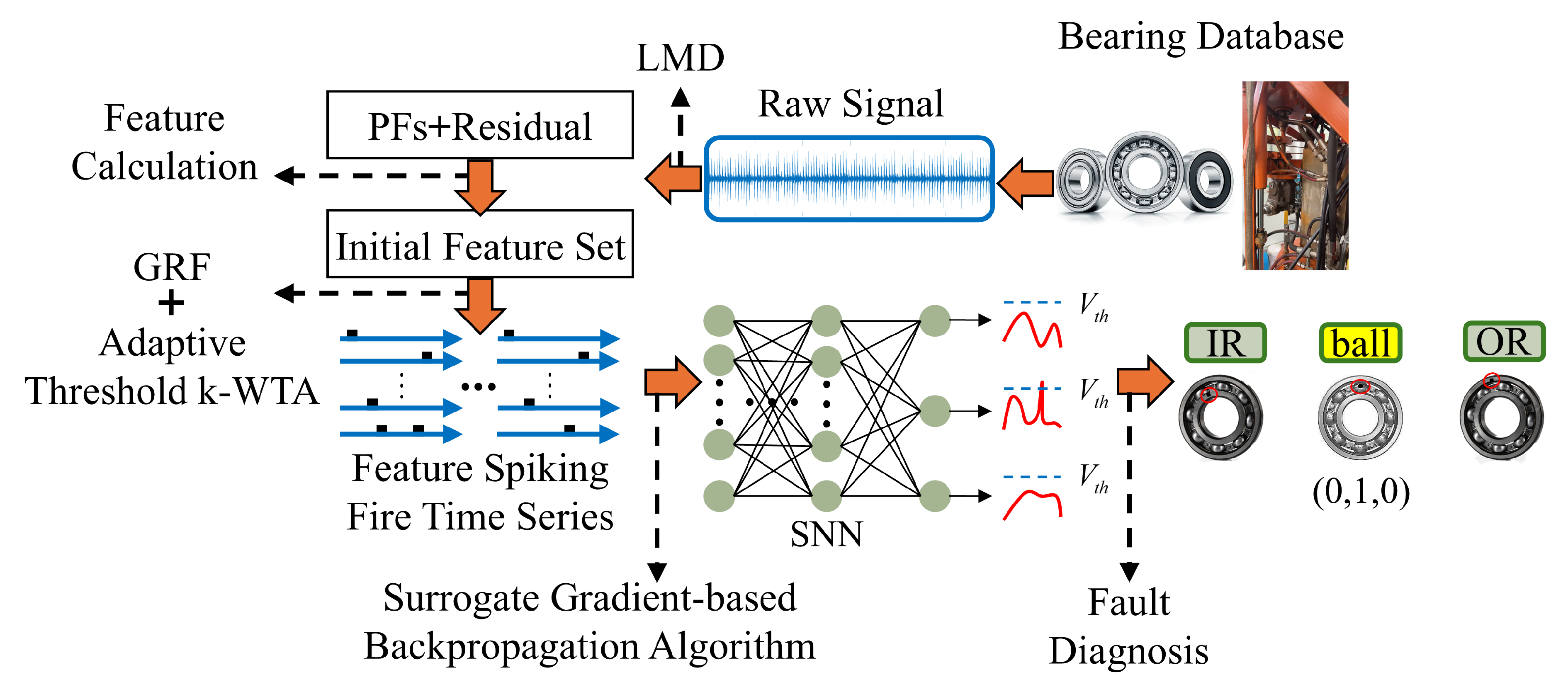
Figure 2.
LMD extracted PFs and residual signal from CWRU data.
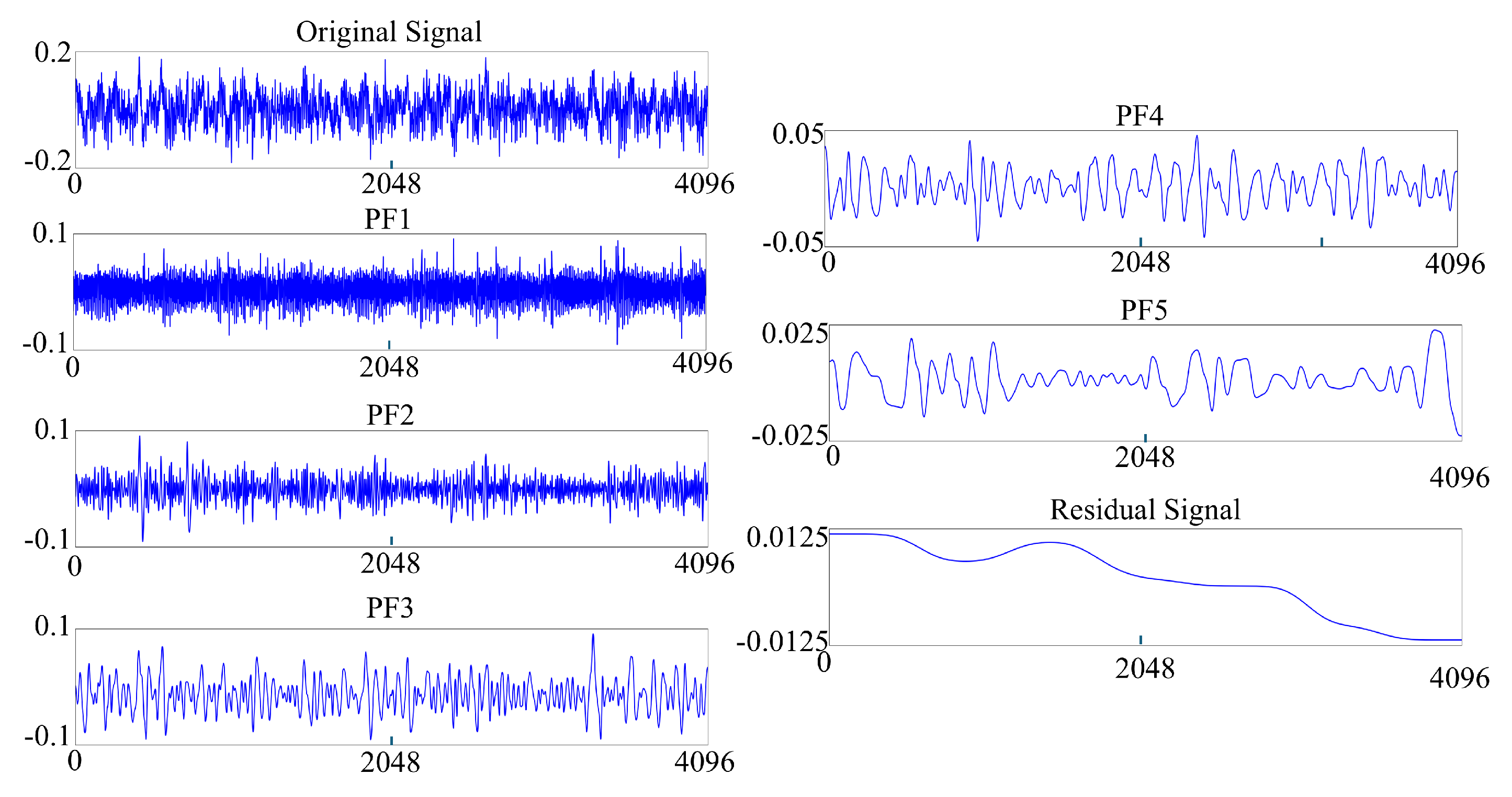
Figure 5.
The test rig used by the Paderborn University datase [34].
Figure 5.
The test rig used by the Paderborn University datase [34].
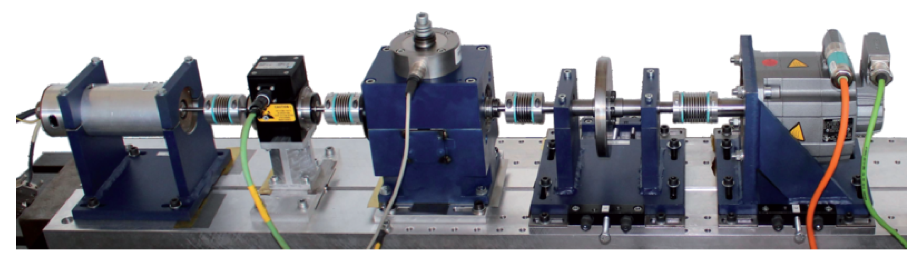
Figure 6.
Subsea drilling rig main shaft condition simulation test bench.
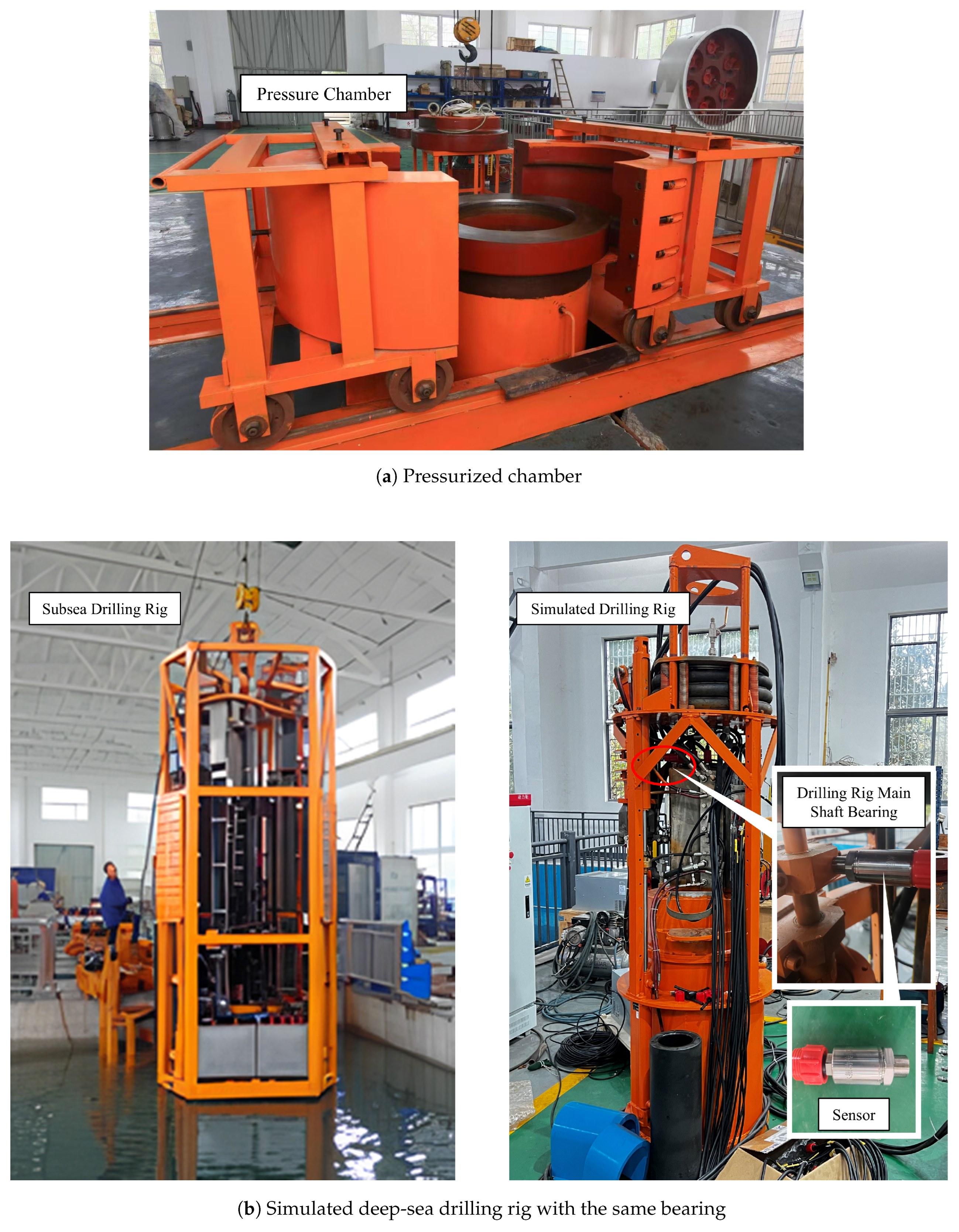
Figure 7.
T-SNE-based Fault Feature Visualization for the CWRU Dataset (Result of 5-Fold Cross-Validation).
Figure 7.
T-SNE-based Fault Feature Visualization for the CWRU Dataset (Result of 5-Fold Cross-Validation).
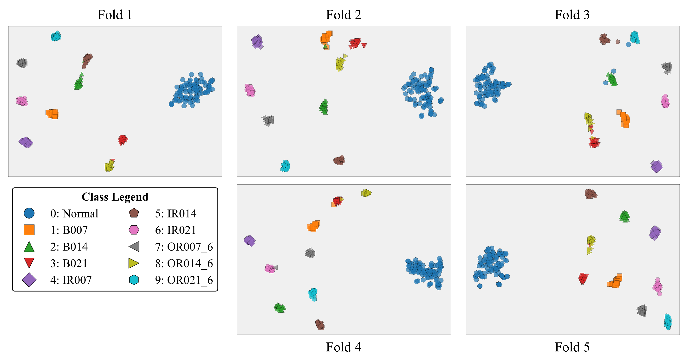
Figure 8.
T-SNE-based Fault Feature Visualization for the Paderborn University dataset (Result of 5-Fold Cross-Validation).
Figure 8.
T-SNE-based Fault Feature Visualization for the Paderborn University dataset (Result of 5-Fold Cross-Validation).
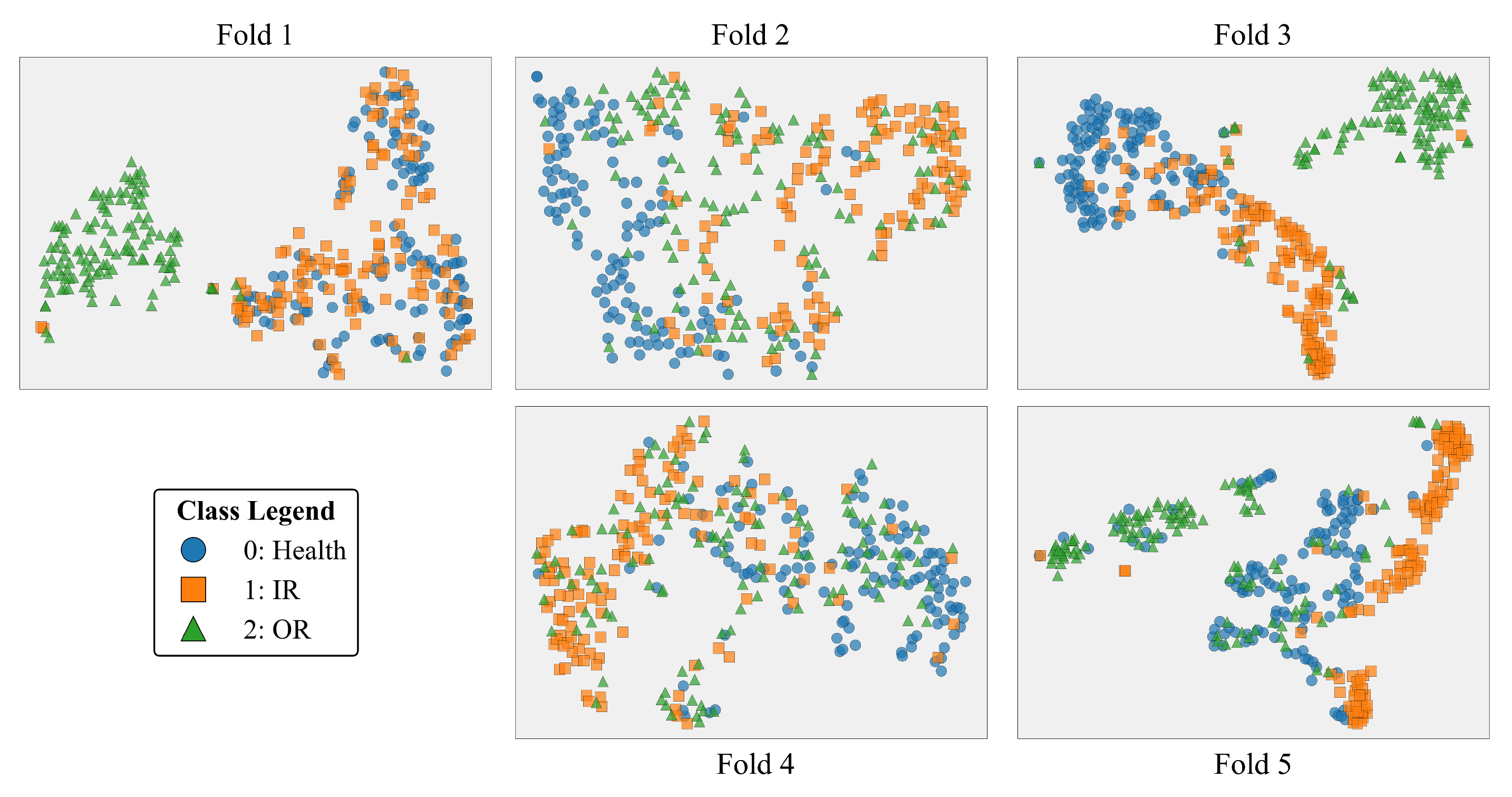
Figure 9.
Aggregated 5-fold cross-validation confusion matrix for the PU dataset.
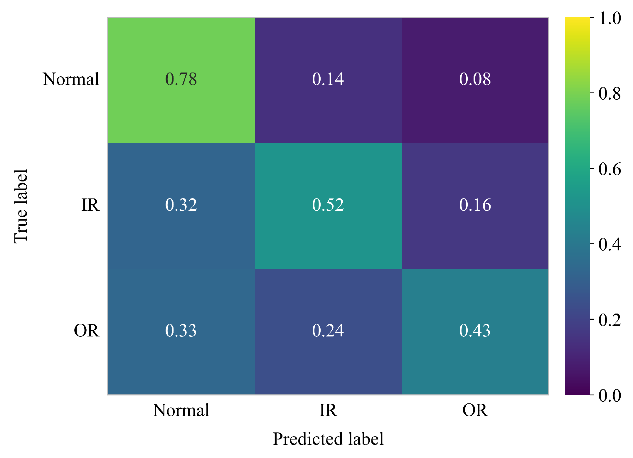
Figure 10.
Noise robustness comparison of different methods on the CWRU dataset.
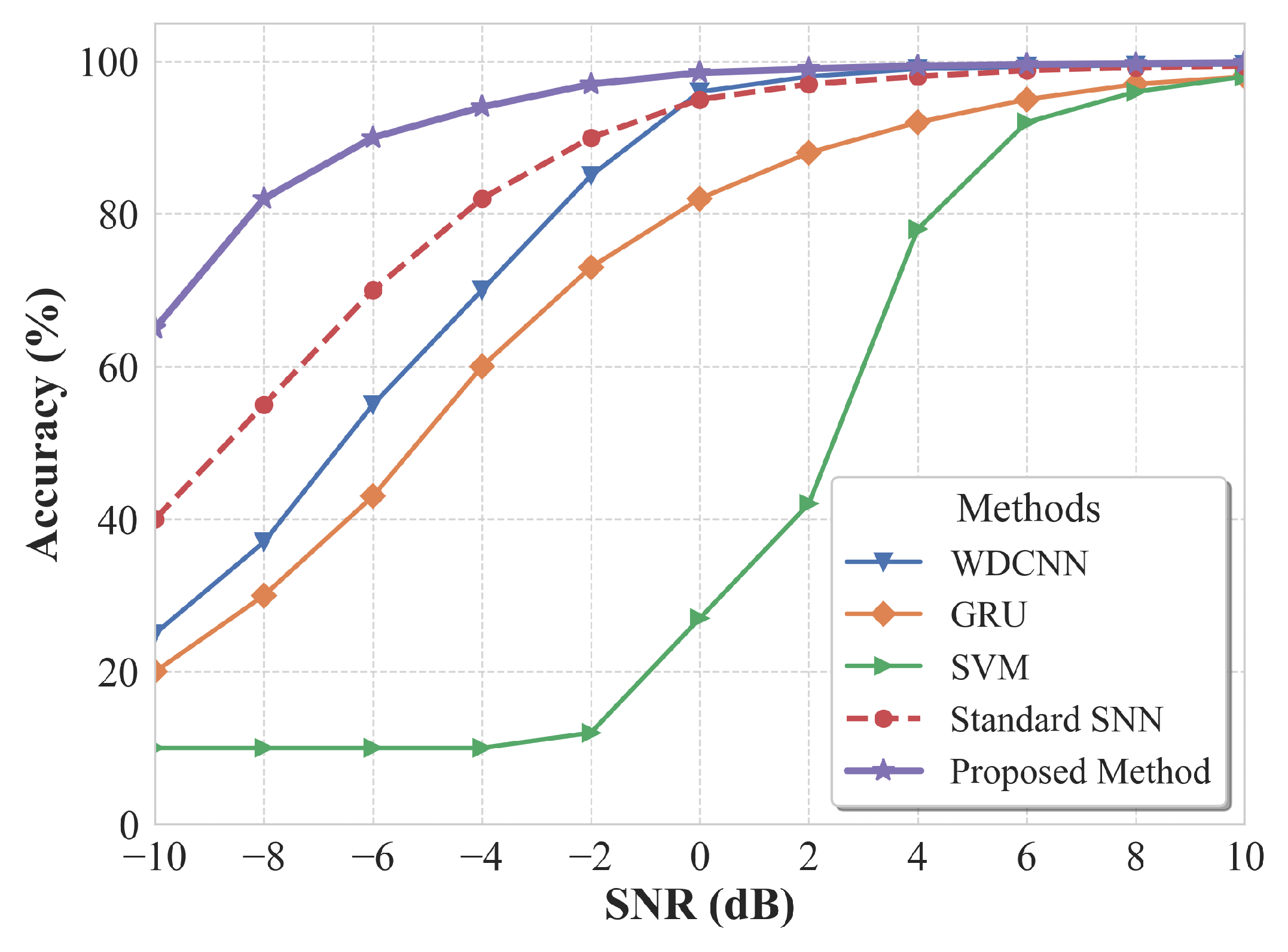
Figure 11.
Aggregated 5-fold cross-validation confusion matrix for the self-collected dataset.
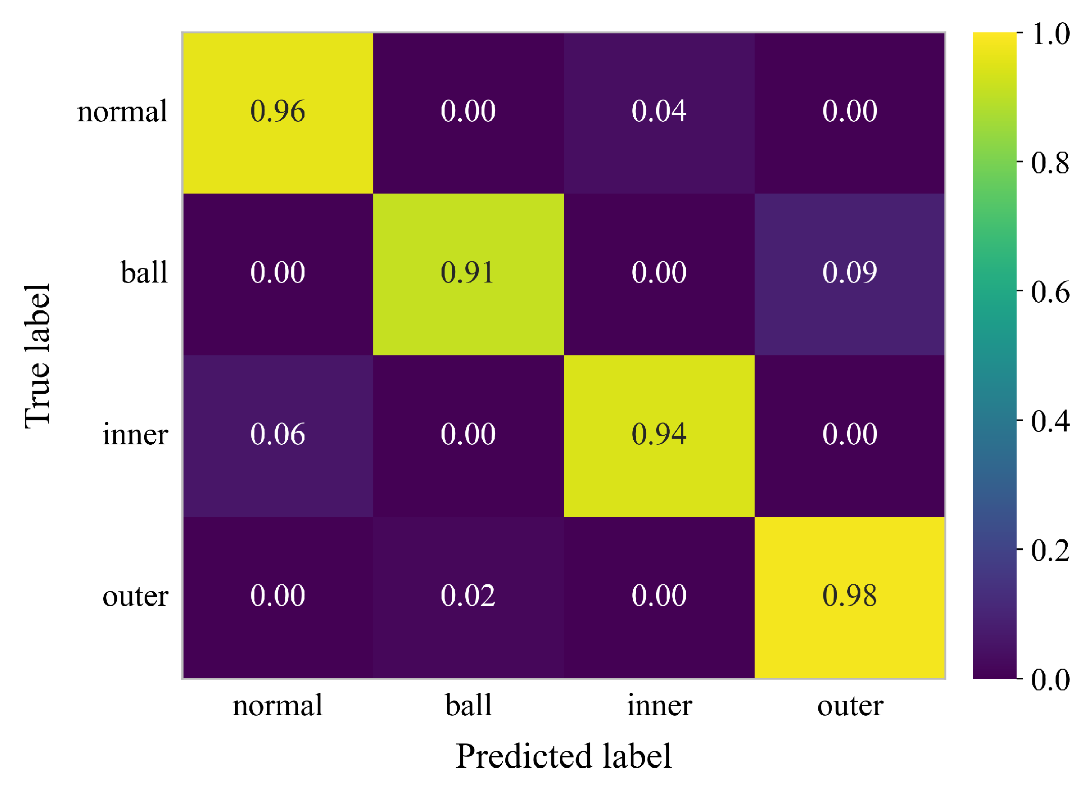
Figure 12.
T-SNE-based Fault Feature Visualization for the self-built dataset (Result of 5-Fold Cross-Validation).
Figure 12.
T-SNE-based Fault Feature Visualization for the self-built dataset (Result of 5-Fold Cross-Validation).
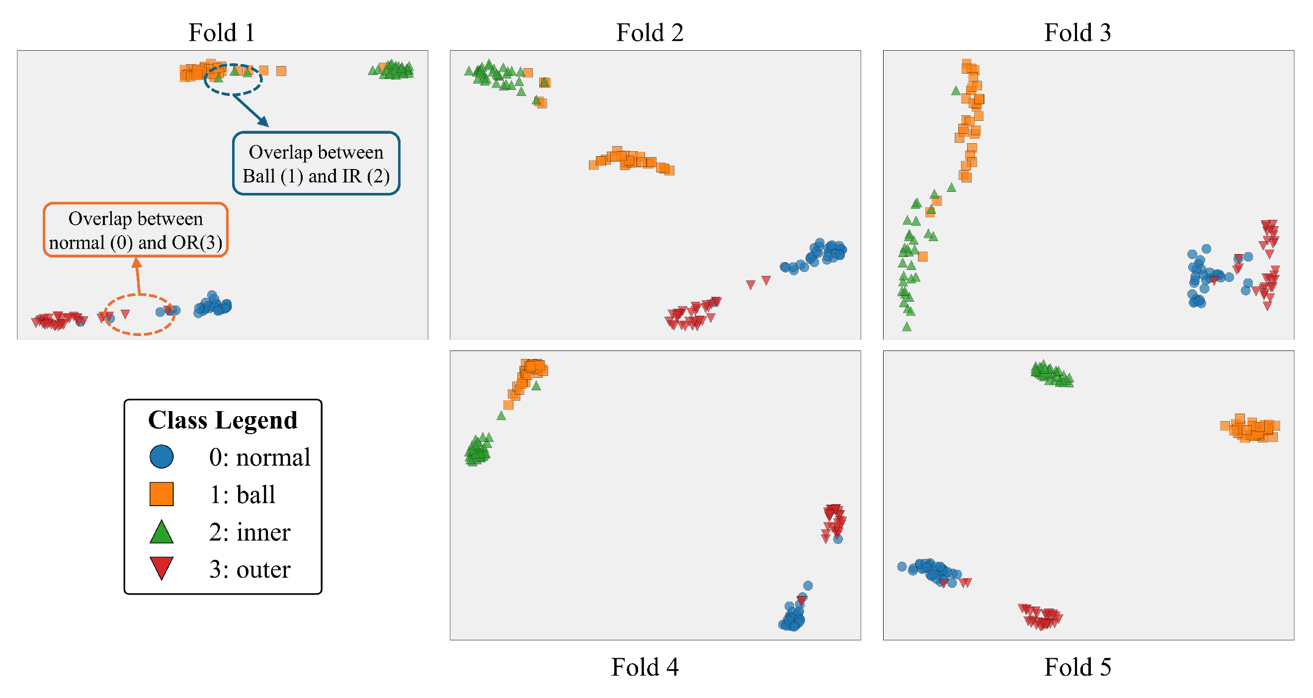
Figure 13.
Energy consumption comparison.
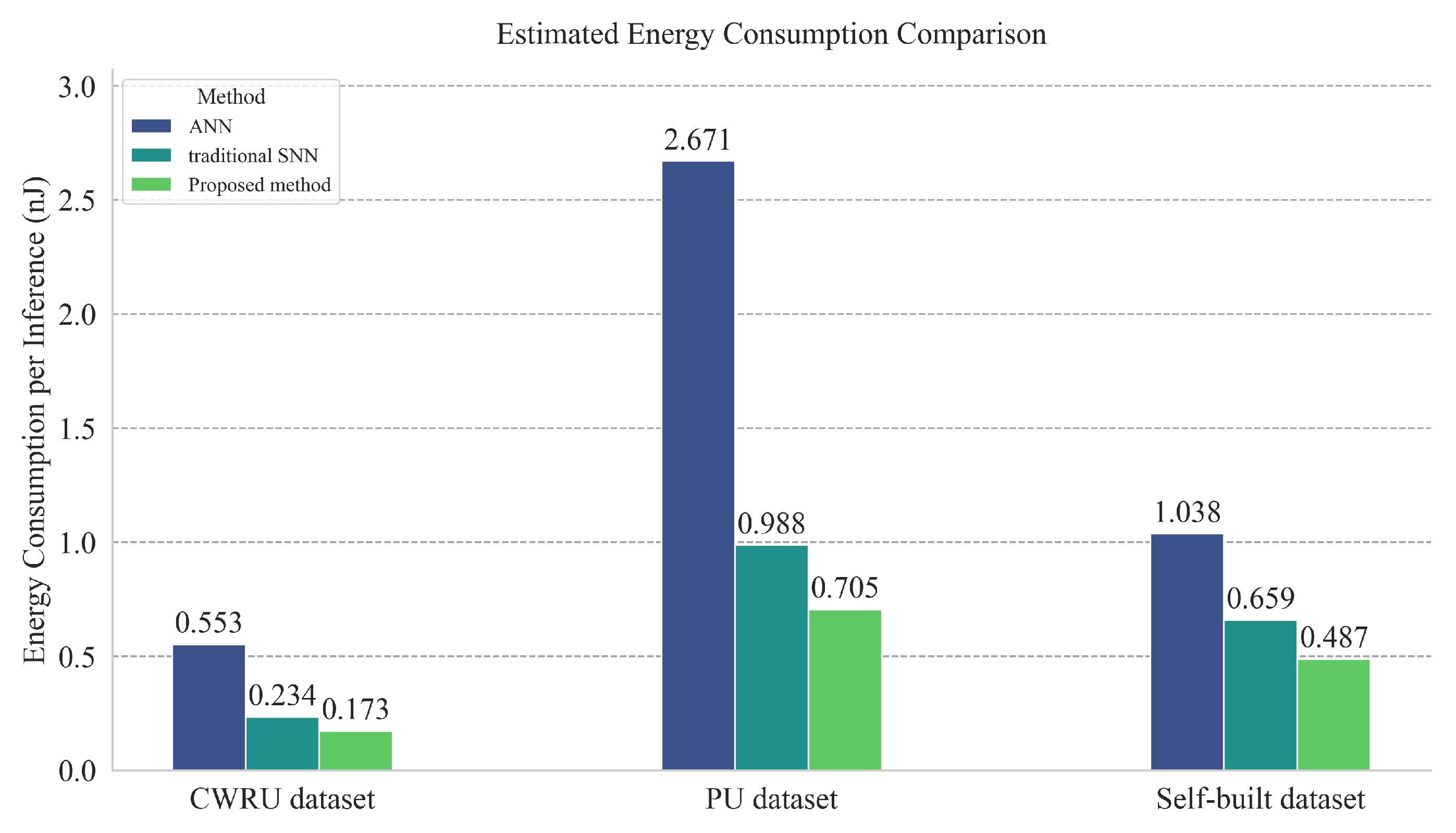

Table 1.
The statistical features derived from each PF component.
| Feature | Mathematical Formulation |
| Kurtosis | |
| Crest Factor | |
| Impulse Factor | |
| Spectral Energy | |
| Spectral Kurtosis |
Table 2.
Sample bearings from the CWRU dataset.
| Bearing code | Bearing label | Sample size | Bearing code | Bearing label | Sample size |
|---|---|---|---|---|---|
| Normal | 0 | 100 | IR014 | 5 | 100 |
| B007 | 1 | 100 | IR021 | 6 | 100 |
| B014 | 2 | 100 | OR007_6 | 7 | 100 |
| B021 | 3 | 100 | OR014_6 | 8 | 100 |
| IR007 | 4 | 100 | OR021_6 | 9 | 100 |
Table 3.
The samples chosen from the real damaged bearings.
| Bearing code | Bearing name | Bearing code | Bearing name | Bearing code | Bearing name |
|---|---|---|---|---|---|
| K001 | H1 | KI04 | IR1 | KA04 | OR1 |
| K002 | H2 | KI14 | IR2 | KA15 | OR2 |
| K003 | H3 | KI16 | IR3 | KA16 | OR3 |
| K004 | H4 | KI18 | IR4 | KA22 | OR4 |
| K005 | H5 | KI21 | IR5 | KA30 | OR5 |
Table 4.
Geometric parameters of the bearing.
| Parameter | Symbol | Value |
|---|---|---|
| Pitch diameter | ||
| Roller diameter | d | |
| Contact angle | ||
| Number of rollers | Z | 10 |
Table 5.
Diagnostic accuracy (%) across the 5-folds of the CWRU dataset.
| Fold Index | 1 | 2 | 3 | 4 | 5 |
|---|---|---|---|---|---|
| Training | 100.00 | 99.92 | 100 | 99.75 | 99.92 |
| Testing | 99.95 | 99.94 | 99.97 | 99.95 | 99.63 |
Table 6.
Comparison of diagnostic accuracy on the CWRU bearing dataset.
| Model | Accuracy (%) | Reference |
| Diagnosisformer | [38] | |
| PSRM | [27] | |
| VKCNN | [39] | |
| Proposed Method | — |
Table 7.
Accuracy per fold on the Paderborn dataset (%).
| Fold Index | 1 | 2 | 3 | 4 | 5 |
|---|---|---|---|---|---|
| Training | 70.16 | 73.66 | 67.67 | 70.03 | 75.54 |
| Testing | 64.78 | 56.45 | 73.92 | 56.18 | 36.02 |
Table 8.
Accuracy per fold on the self-built dataset (%).
| Fold Index | 1 | 2 | 3 | 4 | 5 |
|---|---|---|---|---|---|
| Training | 95.80 | 96.60 | 97.99 | 98.60 | 98.52 |
| Testing | 93.70 | 95.28 | 94.06 | 96.83 | 96.75 |
Disclaimer/Publisher’s Note: The statements, opinions and data contained in all publications are solely those of the individual author(s) and contributor(s) and not of MDPI and/or the editor(s). MDPI and/or the editor(s) disclaim responsibility for any injury to people or property resulting from any ideas, methods, instructions or products referred to in the content. |
© 2025 by the authors. Licensee MDPI, Basel, Switzerland. This article is an open access article distributed under the terms and conditions of the Creative Commons Attribution (CC BY) license (http://creativecommons.org/licenses/by/4.0/).
Copyright: This open access article is published under a Creative Commons CC BY 4.0 license, which permit the free download, distribution, and reuse, provided that the author and preprint are cited in any reuse.


