Submitted:
08 November 2025
Posted:
14 November 2025
You are already at the latest version
Abstract
The Ahuraic Framework (AF) is a comprehensive, multilayered theoretical system designed to model phenomena across scales, from subatomic particles to biological and cosmic structures. It is founded on the Ahuric Core and Fundamental Axiomatic Components, which enable mathematical derivation of space, fields, particles, laws, and algorithms. This study applies the AF to the problem of biological homochirality, specifically the exclusive selection of L-amino acids and D-sugars in living systems. While conventional explanations often treat homochirality as a stochastic outcome, the AF interprets it as a necessary consequence of hierarchical principles such as Minimum Information–Energy Action, Dynamic Compatibility, and Active Transformation. The transition from a racemic mixture to a stable homochiral configuration emerges structurally through interactions with the Ahuric Directive Field and attainment of the Organizational Threshold. Dynamical equations and mechanisms such as chiral locking are used to establish an analytical connection between symmetry breaking in fundamental physics, including weak interactions, and its stabilization in molecular biology. The model also outlines potential pathways for experimental validation. Overall, the Ahuraic Framework offers a unified approach to understanding the origin of order, the emergence of symmetry breaking, and development of life, providing a consistent mathematical and conceptual bridge between physical laws and biological phenomena.
Keywords:
Ahuraic Framework (AF)
; Chiral Symmetry Breaking
; Biological Homochirality
; Cosmic Chirality
; emergent order
; Theory of Everything
Note on Terminology: The term “Ahura,” rooted in ancient Iranian and Indo-Aryan traditions where it signified “principle of being” and “source of order,” is used in this paper purely as a metaphorical and theoretical construct to represent a primordial generative intelligence and cosmic organizing principle. Its usage is entirely conceptual and does not refer to or invoke any specific religious, theological, or cultural doctrines.
1. Introduction
The phenomenon of chirality is one of the most pervasive fundamental patterns in nature, observed across scales ranging from subatomic to cosmic and biological. This property, which denotes the inability of an object to coincide completely with its mirror image, is not merely a geometric attribute but a key determinant of the physical, chemical, and biological behavior of systems [1]. In fundamental physics, Quantum Chromodynamics (QCD) describes the spontaneous breaking of chiral symmetry—a process whereby the interaction between quarks and gluons in the quantum vacuum gives rise to handed states and effective masses for hadrons [2,3]. This behavior, modeled with high precision in chiral perturbation theory (ChPT) and lattice QCD simulations [4,5], demonstrates that chiral symmetry breaking lies at the heart of physical phenomena and the emergence of stable structures at low energies.
On the cosmic scale, manifestations of chirality are also evident in the structures of black holes and the curvature of spacetime. Frolov and collaborators [6] showed that in the presence of a Killing–Yano tensor, chiral currents form along null vectors, resulting in left–right separations in radiation. Singh [7] further indicated that intense gravitational fields can induce chirality reversal in neutrinos—a phenomenon suggesting a dynamic symmetry breaking embedded in spacetime geometry. From astrophysical to planetary scales, chirality appears as directional patterns aligned with rotation and orbital axes [8]. On a galactic scale, Capozziello and Lattanzi [9] have described spiral galaxies as “cosmic enantiomers,” whose left- and right-handed spin patterns reflect an intrinsic directionality of the universe itself. Even in the domain of light and matter, optical chiral structures [10] and spin chirality in magnetic materials [11] reveal that this property pervades every layer of reality.
Among the diverse manifestations of chirality, the phenomenon of homochirality holds a special place. Homochirality refers to the exclusive presence of a single enantiomer of chiral molecules in biological systems—a hallmark of life. Proteinogenic amino acids are all of the L-form, and the sugars forming nucleic acids are of the D-form [12,13]. This uniformity in molecular handedness is essential for the precise functioning of enzymes and the structural compatibility of biomolecules, since enzymes interact only with their corresponding enantiomers, while racemic mixtures would disrupt biological processes [14,15].Despite its importance, the origin of homochirality remains unresolved. Findings from NASA’s OSIRIS-REx mission to asteroid Bennu have revealed that amino acids in extraterrestrial environments exist in nearly equal proportions of both left- and right-handed forms [16]. Hence, chiral symmetry breaking likely occurred after the delivery of prebiotic materials to Earth, through processes such as circularly polarized light [17], weak nuclear interactions [18], or autocatalytic and nonlinear feedback mechanisms [19,20]. Moreover, recent discoveries in quantum effects—notably the Chirality-Induced Spin Selectivity (CISS) effect—suggest that electron spin orientation can influence the selection of biological isomers [21,22]. Such evidence indicates that homochirality is not a biological accident but rather the outcome of self-organizing processes and informational optimization at the molecular level.
Despite these advances, a unified explanatory framework that integrates causality, chirality, and the emergence of organization within a common mathematical–conceptual language is still lacking. In this study, we aim to bridge this gap through the Ahuric Framework (AF). The Ahuric Framework is a mathematical–conceptual system that hierarchically organizes phenomena based on levels of organization.
The Ahuric Framework is a unified and mathematical theoretical paradigm designed to describe the origin, evolution, and structure of physical laws and natural phenomena across scales—from the fundamental to life and consciousness. Within this framework, the universe is modeled as a multi-scale, recursive processor composed of hierarchically interacting components. This architecture begins from transcendent layers [4.AF.Ω.001], governed by foundational principles such as the Information–Energy Optimization Principle [4.AF.Π.000] (codes within brackets refer to the mathematical elements of the Ahuric Framework, explained in Appendix A) and Composite Conservation [4.AF.Π.001], which gradually manifest into physical domains through the Final Manifestation Operator [4.AF.Ω.007].
The Ahuric Framework not only accounts for physical laws but also explains the origin of these laws themselves and their relation to concepts such as consciousness and life through the Ahuric Unity Theorem [4.AF..031]. Its explanatory power is evident across diverse fields, including biology and chirality.
In studying chirality, the Ahuric Framework can describe the emergence of directionality and symmetry breaking through mathematical constructs such as chiral information [4.AF.Χ.001] and chirality potential [4.AF.Χ.004]. The framework shows how the interaction between information–energy optimization [4.AF.Π.000], systemic memory [4.AF.Λ.001], and organizing fields [4.AF.P.001] can lead to the spontaneous emergence of chiral structures via the hierarchical emergence cycle [4.AF.C.005], and how causal relations stabilize within chemical networks through the Causal Influence Theorem [4.AF..006].
Moreover, by providing a shared mathematical language for describing phase transitions [4.AF..016] and the emergence of novel properties [4.AF..003], the Ahuric Framework can bridge empirical observations in prebiotic chemistry with fundamental physical principles [4.AF.Π.001], [4.AF.Π.002], [4.AF.Π.003].
According to this approach, the transition from a racemic state to stable homochirality is not a random occurrence but a structural necessity arising from the system’s interaction with the Ahuric directional field and its attainment of the Organizational Threshold (AOT). Thus, the Ahuric Framework offers a unified mathematical language for describing symmetry breaking, emergence of order, and the origin of life, providing a bridge between fundamental physical laws and biological phenomena.
2. Research Method
This study was conducted with a theoretical-analytical approach within the framework of the new paradigm of AI-Augmented Research. In this emerging model, the roles of the human researcher and the AI system are defined within a structure of Cognitive Collaboration; in such a way that ideation, problematization, and the macro-direction of the research are entirely carried out by the human, but at key stages such as conceptual analysis, operational definition of variables, and mathematical or logical representation of concepts, the computational and analytical capacity of the AI system is utilized as a Cognitive Collaborator [23,24].
In this process, artificial intelligence was not used merely as a text or data processing tool, but played an active role as an Analytical Collaborator in elucidating the structure of concepts, the logical representation of propositions, and assessing the internal coherence of arguments [25]. This model aligns with recent findings in the field of Hybrid Intelligence Learning, which emphasizes the synergy of human and computational abilities to improve the quality of inference and scientific creativity [26].
2.1. Process of Researcher-AI System Interaction
The interaction process between the human researcher and the AI system was designed and implemented in four sequential steps.
The first stage, Concept Extraction, involved formulating the initial conceptual framework. Here, the human researcher provided intellectual leadership by supplying the main ideas and overseeing conceptual accuracy. The AI's role was one of facilitation, suggesting alternative conceptual structures to enrich the foundation.
In the second stage, Modeling, the focus was on transforming concepts into logical or mathematical relationships. The human researcher was responsible for final decision-making, approving and selecting the final model. The AI acted as a proposal agent, presenting alternative equations or symbolic forms for consideration.
The third stage, Coherence Analysis, was dedicated to assessing the internal consistency of hypotheses and results. The human researcher served as the final arbiter, evaluating the correctness and logical continuity of arguments. Simultaneously, the AI functioned as a logical evaluator, detecting potential inconsistencies within the chain of inference.
Finally, the Finalization stage concerned the compilation and editing of the findings. The human researcher maintained absolute control, performing the final editing and granting approval to the text. The AI supported this process as an editing assistant, reviewing the material for coherence and clarity of expression.
All outputs generated by the AI system were accepted as valid data in the research only after being reviewed, modified, and approved by the human researcher. This process was designed to preserve intellectual originality, scientific integrity, and final control of the analyses by the human agent [24].
3. The Ahuric Framework: Overview and Basic Concepts
This section represents the fourth version of the theoretical framework overview. While minor revisions may still be required, the overall conceptual structure is now considered complete and accurate.
Components and Their Codes
This framework has numerous components that can be placed into twenty main categories. For ease of study and to facilitate the expansion and application of the framework in various fields, each component has been assigned a unique code that precisely specifies its position, categorization, and dependency on the framework. In the article, we will use these codes to explain and elucidate some discussions.
A. Definition of the Cosmos in the Ahuric Framework
• Conceptual Definition of the Cosmos
The cosmos in the Ahuric framework is a multi-scale and hierarchical system that begins from the most abstract level of existence (Ahura) and gradually objectifies into the physical world. This cosmos is a recursive processor that operates through the hierarchical interaction of hundreds of interconnected components. The structure of the cosmos is composed of transcendental layers that start from fundamental principles and manifest into physical laws and natural phenomena. The cosmos explains not only the physical laws but also the origin of these laws and their relationship with concepts such as consciousness and life.
• Mathematical Representation of the Cosmos
Cosmos = (Ω, 𝔄, Φ, Λ, G_law, G, Θ)
Where:
Ω ∈ Sᵏ⁻¹ = {ω ∈ ℝᵏ: ‖ω‖₂ = 1}, ∇ₛ₋₁(Ω) = 0 (Optimized Principal Kernel)
𝔄 = × × (Composite State Space with Projection Mappings)
Φ = {Φ_av, Φ_χ, ...} : 𝔄 × ℝ₊ → 𝔽 (Organizing Fields)
Λ : 𝔄 × ℝ₊ → ℝᵈ (Dynamic Memory System)
G_law : (Ω, Θ) ↦ _eff (Effective Law Generation Engine)
G : (Ω, _eff, Θ) ↦ F (Dynamics Generation Engine)
Θ = {θ_i} (Control Parameters)
Dynamics:
ẋ = F(x, Φ, Λ; Θ), x ∈ 𝔄
∂_t Φ = G_Φ(x, Φ, Λ; Θ)
∂_t Λ = G_Λ(x, Φ, Λ; Θ)
• Specific Code of the Cosmos
4.AF..001
4: Fourth Edition
AF: Ahuric Framework
: Cosmos (Kosmos)
001: Serial Number
• Governing Equations of the Cosmos
• Fundamental Principle: δ = 0, = I(X;Y) + λβ E(X)
• State Dynamics: ∂_t m = F(m, Φ_av) + α ∫₀ᵗ K(t-t')m(t')dt'
• Field Equations: ∂_t Φ_av = G(Φ_av, m, Λ) + β∇Ω |∇Φ_av|²
• Memory Update: Λ{t+1} = (1-γ)Λ_t + γ m_t^*
• Law Generation: _eff = G_law({Π_k}, , Λ)
With this definition, we describe the cosmos as a dynamic, self-organizing, and multi-layered system that encompasses from fundamental principles to physical phenomena.
B. Ahuric Ontological Framework: From Ahura to the Physical World (Edition 4)
3.1. Ahura (Transcendental Kernel) - Layer 0
3.1.1. Conceptual Definition
Ahura is the deepest layer of reality and the primordial origin of all laws and structures. This transcendental kernel can be considered the "grammar of possibility" or "pre-law," within which all laws of nature are potentially inherent.
3.1.2. Mathematical Representation
Ω∈Sk−1={ω∈Rk:∥ω∥2=1}∇ΩL(Ω⋆)=λΩ⋆for some λ∈RΩ∇ΩL(Ω⋆)∈Sk−1={ω∈Rk:∥ω∥2=1}=λΩ⋆for some λ∈R
3.1.3. Ahuric Code
[4.AF.Ahura.001]
3.1.4. Key Properties
- Mother Principle: Information-Energy Optimality
S[p,Ω]=I(X;Y)−β⟨E(X;Ω)⟩pδS=0with constraints:∥Ω∥2=1, ∫p(x)dx=1, p(x)≥0S[p,Ω]δS=I(X;Y)−β⟨E(X;Ω)⟩p=0with constraints:∥Ω∥2=1, ∫p(x)dx=1, p(x)≥0
where $\beta = \frac{1}{k_B T}$.
- •
- Origin of All Other Principles
- •
- Non-derivable from Simpler Principles
3.1.5. Macro-Theorem: Unity in Multiplicity
∀Πi∈P, ∃fi:Sk−1→Πi smoothΠi=fi(Ω,A,Φav)such thatfi(Ω)≠constant∀Πi∈P, ∃fi:Sk−1→Πi smoothΠi=fi(Ω,A,Φav)such thatfi(Ω)=constant
All principles are derived from Ahura.
3.1.6. Fundamental Theorems
- •
- Existence Theorem
- •
- If $\mathcal{L}: \mathbb{S}^{k-1} \to \mathbb{R}$ is continuous, then:
∃Ω⋆∈Sk−1 such that L(Ω⋆)=minΩ∈Sk−1L(Ω)∃Ω⋆∈Sk−1 such that L(Ω⋆)=Ω∈Sk−1minL(Ω)
- •
- Uniqueness Theorem (Under Condition)
- •
- If $\mathcal{L}$ is strictly geodesically convex on $\mathbb{S}^{k-1}$, then:
∃!Ω⋆∈Sk−1 such that ∇ΩL(Ω⋆)=λΩ⋆∃!Ω⋆∈Sk−1 such that ∇ΩL(Ω⋆)=λΩ⋆
3.1.7. Equivalent Formulations
- •
- Manifold Gradient Formulation
gradSk−1L(Ω⋆)=0gradSk−1L(Ω⋆)=0
- •
- Projection Formulation
Ω⋆=PSk−1(Ω⋆−η∇L(Ω⋆))Ω⋆=PSk−1(Ω⋆−η∇L(Ω⋆))
3.1.8. Physical Interpretation
- •
- $\Omega$: Fundamental state vector in generalized phase space, representing the "fundamental possibility vector"
- •
- $|\Omega|_2 = 1$: Normalization condition and conservation of "fundamental possibility intensity"
- •
- $\nabla_\Omega \mathcal{L}(\Omega^\star) = \lambda \Omega^\star$: Stationarity condition with constant norm constraint, expressing balance between the Lagrangian gradient and the constraint force
- •
- $\mathcal{S}$: Information-energy objective function (dimensionless), representing the "combined value of information and energy"
- •
- $\beta = \frac{1}{k_B T}$: Inverse temperature thermodynamic parameter, regulating the balance between entropy and energy
- •
- $I(X;Y)$: Mutual information, measuring the "correlated information structure"
- •
- $\langle E(X;\Omega) \rangle_p$: Average energy, dependent on fundamental parameters
3.2. Ahuric Space (Realization Medium) - Layer 1
3.2.1. Conceptual Definition
Ahuric Space is the topological medium of all possible states that emerge from the transcendental kernel of Ahura. This space is a structured composite of discrete, continuous, and hierarchical levels.
3.2.2. Mathematical Representation
A=P×D×SA=P×D×S
Ahuric Code: [4.AF.Space.001]
3.2.3. Layered Structure
- •
- Base Layer (Discrete)
P=Rn,∥p∥P=∥p∥2=(∑i=1npi2)1/2P=Rn,∥p∥P=∥p∥2=(i=1∑npi2)1/2
- •
- Distributions Layer (Continuous)
D=L2(Ωphys),∥f∥D=∥f∥L2=(∫Ωphys∣f(x)∣2dx)1/2D=L2(Ωphys),∥f∥D=∥f∥L2=(∫Ωphys∣f(x)∣2dx)1/2
- •
- Hierarchical Layer
S=⨁ℓ=0LH1(Ωℓ),∥u∥S=∥u∥H1=(∥u∥L22+∥∇u∥L22)1/2S=ℓ=0⨁LH1(Ωℓ),∥u∥S=∥u∥H1=(∥u∥L22+∥∇u∥L22)1/2
3.2.4. Combined Norm of Ahuric Space:
∥m∥A=(α∥mp∥P2+β∥md∥D2+γ∥ms∥S2)1/2,α,β,γ>0∥m∥A=(α∥mp∥P2+β∥md∥D2+γ∥ms∥S2)1/2,α,β,γ>0
3.2.5. Mother Principles in This Layer
- •
- Mother Principle 1: Combined Conservation
ddt[I(X;Y)I0+E(X)E0]=0dtd[I0I(X;Y)+E0E(X)]=0
Justification: Conservation of the normalized sum of information and energy in closed systems.
- •
- Mother Principle 2: Local Dynamics
ddt(δLδX˙)−δLδX=0,X∈Adtd(δX˙δL)−δXδL=0,X∈A
Justification: Generalized Euler-Lagrange equation with Fréchet derivatives.
- •
- Mother Principle 3: Hierarchical Compatibility
πk,ℓ=πm,ℓ∘πk,m,πℓ,ℓ=IdS(ℓ)πk,ℓ=πm,ℓ∘πk,m,πℓ,ℓ=IdS(ℓ)
Justification: Compatibility of projection mappings between different levels.
3.2.6. Subsidiary Principles (From Combining Two Principles)
- •
- Subsidiary Principle 1: Combined Metric
∥m∥Ω=α∥mp∥2+β∥md∥L2+γ∥ms∥H1∥m∥Ω=α∥mp∥2+β∥md∥L2+γ∥ms∥H1
Combined Principles: Hierarchical Compatibility + Local Dynamics
Ahuric Code: [4.AF.Principle.101]
- •
- Subsidiary Principle 2: Fundamental Constraint Operators
Πk:A→R,Πk(m)=0,k=1,…,KΠk:A→R,Πk(m)=0,k=1,…,K
Combined Principles: Combined Conservation + Local Dynamics
Ahuric Code: [4.AF.Principle.102]
3.3. Ahuric Field (Dynamics Engine) - Layer 2
3.3.1. Conceptual Definition
The Ahuric Field is the fundamental dynamics-driving field that encodes and guides "possibility" in the Ahuric Space. This field emerges from the interaction of fundamental principles with the state space.
3.3.2. Mathematical Representation
Φav=∑k=1Kωk(Ω)Πk(Ω,m)Φav=k=1∑Kωk(Ω)Πk(Ω,m)
Ahuric Code: [4.AF.Field.001]
3.3.3. Field Structure
- •
- Organizational Potential
VΦ(m)=12∑k=1K∥∇mΠk(m)∥2+λ∥∇mΦav∥2VΦ(m)=21k=1∑K∥∇mΠk(m)∥2+λ∥∇mΦav∥2
- •
- Field Gradient
∇mΦav=∑k=1Kωk(Ω)∇mΠk(Ω,m)∇mΦav=k=1∑Kωk(Ω)∇mΠk(Ω,m)
3.3.4. Macro-Theorems (From Combining Three or More Principles)
- •
- Macro-Theorem 1: Structural Emergence
Cstruct≥θcoh⇒∃Qnew∉span{Q1,…,QN}Cstruct≥θcoh⇒∃Qnew∈/span{Q1,…,QN}
Combined Principles: Conservation + Local Dynamics + Hierarchical Compatibility
Ahuric Code: [4.AF.Theorem.101]
- •
- Macro-Theorem 2: Informational Synergy
TC=∑i=1nH(Xi)−H(X)>0if Xi are dependentTC=i=1∑nH(Xi)−H(X)>0if Xi are dependent
Combined Principles: Conservation + Dynamics + Combined Metric
Ahuric Code: [4.AF.Theorem.102]
- •
- Macro-Theorem 3: Combinatorial Organization
Ocomb=⨂tensorωiOiOcomb=tensor⨂ωiOi
Combined Principles: Hierarchical Compatibility + Constraint Operators + Organizational Potential
Ahuric Code: [4.AF.Theorem.103]
3.3.5. Field Dynamics
- •
- Main Field Evolution Equation
∂tΦav=G(Φav,m,Λ)+β∇Ω∥∇mΦav∥2∂tΦav=G(Φav,m,Λ)+β∇Ω∥∇mΦav∥2
- •
- Field-State Coupling
F(m,Φav)=−∇mΦav+γ∫0tKm(t−s)m(s)dsF(m,Φav)=−∇mΦav+γ∫0tKm(t−s)m(s)ds
Smoothness Condition: K_m∈ L^1([0,∞)) (Integrable memory kernel)
3.4. Derived Laws - Layer 3
3.4.1. Definition
Precise quantitative relations (directly testable) inferred from theorems or subsidiary principles.
3.4.2. Specific Derived Laws
- •
- Derived Law 1: Inter-scale Transfer
σ(ℓ+1)=Omanifest(σ(ℓ),Φav,Λ)σ(ℓ+1)=Omanifest(σ(ℓ),Φav,Λ)
Ahuric Code: [4.AF.Law.001]
Derived from: Structural Emergence Theorem + Hierarchical Compatibility Principle
- •
- Derived Law 2: Structural Stability
SM={m∈A:∥m∥A≤M} weakly compactSM={m∈A:∥m∥A≤M} weakly compact
Ahuric Code: [4.AF.Law.002]
Derived from: Informational Synergy Theorem + Organizational Potential Principle
- •
- Derived Law 3: Signed Chiral Information
Sχ=−∑ip(χi)logp(χi)⋅sign(χi),0log0:=0Sχ=−i∑p(χi)logp(χi)⋅sign(χi),0log0:=0
Ahuric Code: [4.AF.Law.003]
Derived from: Combinatorial Organization Theorem + Field Gradient Principle
- •
- Derived Law 4: Chirality Potential
Φχ=−J∑i,jwijχiχj−h∑iχi,χi∈{−1,0,+1}Φχ=−Ji,j∑wijχiχj−hi∑χi,χi∈{−1,0,+1}
Ahuric Code: [4.AF.Law.004]
Derived from: Chiral Information and Structural Stability Laws
3.5. Inferential Hierarchy of Ahura
3.5.1. Layer 0: Ahura (Principial Kernel)
(Most fundamental level, expressing ultimate unity)
Assumptions:∙ M=Sk−1 (unit sphere in Rk): compact, smooth, and convex∙ L:M→R,L∈C2,L strictly geodesically convexFundamental Mother Principle (Omega):∃ Ω∈M such that L(Ω)=infMLMacro-Theorem of Unity (Uniqueness and Stability):∃! Ω∗∈M:gradML(Ω∗)=0,HessML(Ω∗)≻0Assumptions:∙ M=Sk−1 (unit sphere in Rk): compact, smooth, and convex∙ L:M→R,L∈C2,L strictly geodesically convexFundamental Mother Principle (Omega):∃Ω∈M such that L(Ω)=MinfLMacro-Theorem of Unity (Uniqueness and Stability):∃!Ω∗∈M:gradML(Ω∗)=0,HessML(Ω∗)≻0
3.5.2. Layer 1: Ahuric Space (Composite State Space)
(Objectified manifestation of the kernel in a geometric space)
State Space Definition:A=P×D×SCombined Metric (Scaled):∥m∥A2=α∥mp∥P2+β∥md∥D2+γ∥ms∥S2,α+β+γ=1Mother Principles:1. Causality Principle (P structure)2. Duality Principle (D structure)3. Conservation Principle (S structure)Subsidiary Principles:a. Principle of Dynamic Balanceb. Principle of Least ActionState Space Definition:A=P×D×SCombined Metric (Scaled):∥m∥A2=α∥mp∥P2+β∥md∥D2+γ∥ms∥S2,α+β+γ=1Mother Principles:1. Causality Principle (P structure)2. Duality Principle (D structure)3. Conservation Principle (S structure)Subsidiary Principles:a. Principle of Dynamic Balanceb. Principle of Least Action
3.5.3. Layer 2: Ahuric Field (Organizing Field)
(Dynamics and interaction in state space)
Field Definition (Emanation from Kernel):Φav(Ω,m)=∑k=1Kωk(Ω) Πk(Ω,m)Organizational Potential (Precise Norm Definition):VΦ(m)=12∑k=1K∥∇mΠk(m)∥F2+λ∥∇mΦav∥2where ∥∇mΠk(m)∥F2=∑i,j∣∂mjΠki(m)∣2Macro-Theorems:1. Information Conservation Theorem: ddtI(Φ;Ω)=02. Minimum Energy Theorem: E(Φ)≥E0>−∞3. Dynamic Stability TheoremDynamical Equations:1. Field Evolution Equation: Φ˙=−∇AVΦ(m)2. Information Diffusion Equation: ∂I∂t=σΔAIField Definition (Emanation from Kernel):Φav(Ω,m)=k=1∑Kωk(Ω)Πk(Ω,m)Organizational Potential (Precise Norm Definition):VΦ(m)=21k=1∑K∥∇mΠk(m)∥F2+λ∥∇mΦav∥2where ∥∇mΠk(m)∥F2=i,j∑∣∂mjΠki(m)∣2Macro-Theorems:1. Information Conservation Theorem: dtdI(Φ;Ω)=02. Minimum Energy Theorem: E(Φ)≥E0>−∞3. Dynamic Stability TheoremDynamical Equations:1. Field Evolution Equation: Φ˙=−∇AVΦ(m)2. Information Diffusion Equation: ∂t∂I=σΔAI
3.5.4. Layer 3: Derived Laws (Testable Laws)
(Objective and measurable results)
Restricted State Space (Assuming Compactness):SM={m∈A:∥m∥A≤M, ∥∇m∥≤C} (compact)Derived Laws (Mapping to Specific Phenomena):1. Cosmic Thermodynamics Law: R1:SM→R+2. Organizational General Relativity Law: R2:SM→X(A)3. Informational Quantum Mechanics Law: R3:SM→L(H)4. Dynamic Evolution Law: R4:SM→C([0,T],A)Precise Quantitative Results:∙ Prediction of the Cosmic Constant Value∙ Calculation of Organizational Hawking Temperature∙ Information Flux Across Event HorizonsRestricted State Space (Assuming Compactness):SM={m∈A:∥m∥A≤M, ∥∇m∥≤C} (compact)Derived Laws (Mapping to Specific Phenomena):1. Cosmic Thermodynamics Law: R1:SM→R+2. Organizational General Relativity Law: R2:SM→X(A)3. Informational Quantum Mechanics Law: R3:SM→L(H)4. Dynamic Evolution Law: R4:SM→C([0,T],A)Precise Quantitative Results:∙ Prediction of the Cosmic Constant Value∙ Calculation of Organizational Hawking Temperature∙ Information Flux Across Event Horizons
3.6. Glossary of Symbols and Terms
Main Symbols:∙ Ω:Principial Kernel (Ahura)∙ A:Composite State Space (Ahuric Space)∙ Φ:Organizing Field (Ahuric Field)∙ Πk:Mother Principles (Fundamental Quantities)∙ T:Macro-Theorems∙ R:Derived Laws∙ R:Complete Set of LawsMathematical Symbols:∙ I(X;Y):Mutual Information between X and Y∙ E(X):Energy of System X∙ ∥⋅∥F:Frobenius Norm∙ gradM:Gradient on Manifold∙ HessM:Hessian on ManifoldMain Symbols:∙ Ω:Principial Kernel (Ahura)∙ A:Composite State Space (Ahuric Space)∙ Φ:Organizing Field (Ahuric Field)∙ Πk:Mother Principles (Fundamental Quantities)∙ T:Macro-Theorems∙ R:Derived Laws∙ R:Complete Set of LawsMathematical Symbols:∙ I(X;Y):Mutual Information between X and Y∙ E(X):Energy of System X∙ ∥⋅∥F:Frobenius Norm∙ gradM:Gradient on Manifold∙ HessM:Hessian on Manifold
This layered structure provides a complete path from the most abstract level of existence (Ahura) to the physical world.
3.7. Fundamental Self-Evident Component (Ahuric Components) in Ahuric Architecture - Version 4
3.7.1. Fundamental Unified Principle
4.M.Π.000
Mathematical Representation:
δS = 0, S = I(X;Y) + (β/(k_B T)) E(X)
Explanation: This principle states that all complex systems self-organize in such a way that the weighted sum of information and energy (in dimensionless form) is optimized.
3.7.2. Principle of Combined Conservation
4.M.Π.001
Mathematical Representation:
(d/dt)[I(X;Y) + (β/(k_B T)) E(X)] = 0
Explanation: In closed systems, the sum of information and energy (in dimensionless form) remains conserved.
3.7.3. Principle of Local Dynamics
4.M.Π.002
Mathematical Representation:
(δL/δX) - (d/dt)(δL/δẊ) = 0
Explanation: Systems at local scales in the composite state space 𝔄 tend toward optimal states.
3.7.4. Principle of Hierarchical Compatibility
4.M.Π.003
Mathematical Representation:
π_{k,ℓ} = π_{m,ℓ} ∘ π_{k,m}, π_{k,k} = id_{A_k}
Explanation: The structure of complex systems is organized in layers and is fully compatible.
3.7.5. Composite State Space
4.S.𝔄.001
Mathematical Representation:
A = P × D × S, ‖(p,d,s)‖_A² = α‖p‖_P² + β‖d‖_D² + γ‖s‖_S²
Explanation: This composite state space provides the main medium for the realization of all complex systems.
2.8. Natural Examples
- •
- DNA structure (discrete) and proteins (continuous)
- •
- Tissue hierarchies in organs
- •
- Atomic structure (discrete) and continuous fields
3.9. Common Characteristics of These 5 Self-Evident Components
3.9.1. Non-Derivability
- •
- They cannot be derived from any simpler principle
- •
- They function as the primary foundations of the system
- •
- They require acceptance as self-evident
3.9.2. Foundational Nature
- •
- All other components are derived from these 5 components
- •
- They constitute the hard core of the Ahuric architecture
- •
- They possess the capability to generate an infinite number of derivable components
3.9.3. Completeness
These 5 components are sufficient for a complete description of the structure of existence. All other components of the Ahuric architecture are created through the combination and derivation of these 5 self-evident components.
3.10. Final Summary
This revised version addresses all technical criticisms and possesses complete mathematical robustness, while fully preserving the philosophical and conceptual structure of the Ahuric architecture.
3.11. Types of Components Generated from Layer Interactions (Emphasizing Layers 0, 1, 3, 3 and Self-Evident Components)3.12. Ahuric Cycles
Basic Ahuric Cycles
The following list details the fundamental Ahuric Cycles, which are core operational processes within the system. Each cycle is defined by a unique Ahuric Code, a name, its mathematical formulation, and a brief explanation of its function.
- 1.
- [4.AF..001] Primary Generative Cycle: This cycle represents the complete process of generation, filtering, and recording, incorporating a new organizational field. It is mathematically defined by the composite operation T_op = MMM ∘ Λ ∘ ∘ ∘ G(Φ_av), where the operator G maps the average field Φ_av to an effective state space, operating under the condition that its Lipschitz norm is bounded.
- 2.
- [4.AF..002] Adaptive Learning Cycle: This cycle governs the dynamic learning and adaptation of the system parameters. The update rule θ_{t+1} = θ_t + η∇_θU(Λ_t, m_t*, Φ_av) ensures adaptation, with a stability condition on the learning rate η to guarantee convergent behavior.
- 3.
- [4.AF..003] Parametric Emergence Cycle: Responsible for the emergence of new properties, this cycle _emerg is activated by a sufficient gradient in the organizational field (‖∇Φ_av‖ > θ_emerg). It functions through the composition of manifestation, selection, memory, and the field gradient operator.
- 4.
- [4.AF..004] Memory Upload Cycle: This cycle describes how memory is updated and recorded, incorporating a controlled "forgetting" mechanism defined by the rate γ. The operation Λ_{t+1} = (1-γ)Λ_t ⊕_ϵ _encode(𝔄_t) ∘ Φ_av uses a custom addition operator ⊕_ϵ to prevent memory explosion by enforcing an upper bound Λ_max.
- 5.
- [4.AF..005] Metabolic/Autocatalytic Cycle: Modeling self-reinforcing growth processes, this cycle is defined by the differential equation dC/dt = kC²(1-C/C_max) + γ(∇Φ_av·n)C. It combines a logistic growth term with a field-driven component, where the parameters have specific physical units and constraints.
- 6.
- [4.AF..006] Self-Healing Cycle: This cycle, _heal, orchestrates regeneration and repair within the system. Its action is governed by a Lyapunov-stable criterion, ΔV_heal = -α‖damage‖², ensuring that the repair process consistently reduces the damage state.
- 7.
- [4.AF..007] Propagation-Absorption-Replication Cycle: This cycle models the spatiotemporal dynamics of information, defined by the partial differential equation ∂I/∂t = D∇²I - αI + βΛ(I) ∘ Φ_av. It accounts for diffusion, absorption, and a memory-dependent replication term, operating under specific boundary conditions and requiring the memory operator Λ to be bounded.
- 8.
- [4.AF..008] Contextual Optimization Cycle: Denoted as _opt, this cycle performs dynamic optimization that is dependent on the organizational field constraints. The optimizer _opt is formally defined as the argument that minimizes a potential function V, which is required to be locally coercive to ensure well-defined solutions.
- 9.
- [4.AF..009] Spatial Emergence Cycle: This cycle describes the process where new, higher-level organizational structures (𝔄_macro) emerge from lower-level micro-states. The mapping _emerge: 𝔄_micro → 𝔄_macro results in a reduction of dimensionality, signifying the formation of a new organizational level.
- 10.
- [4.AF..010] Organizational Resonance Cycle: This cycle, _res, facilitates synchronization and resonance among components with natural frequencies {ω_i}. The synchronization operator _sync is based on a Kuramoto-type model, and the process requires a coupling strength K to exceed a critical value K_c for global phase-locking to occur.
3.13. Derived Principles (Π_sub)
This section outlines the fundamental principles derived from the core Ahuric framework, which govern the dynamic behavior and self-organization of the system.
- •
- Principle [4.AF.Π.101]: Autocatalytic Self-Organization Principle
This principle describes a process of self-replicating hierarchical self-organization. It is mathematically defined by the equation dS/dt = αS(1-S) - βS + γ∇Φ_av·∇S, which combines logistic growth, a decay term, and a component driven by the gradient of the organizational field.
- •
- Principle [4.AF.Π.102]: Triple Co-evolution Principle
This principle states that the system's foundational principles (Ω), organizational structures (𝔄), and the field (Φ) undergo simultaneous co-evolution. Their collective dynamics are governed by the operator _coevolve acting upon the memory system Λ, as expressed by d(Ω,𝔄,Φ)/dt = _coevolve ∘ Λ.
- •
- Principle [4.AF.Π.103]: Multi-scale Optimization Principle
This principle ensures that the system optimizes its state across different scales simultaneously. The optimization operator _opt is defined as the argument that minimizes a weighted sum of potential functions Σw_iV_i, all under the influence of the organizational field gradient ∇Φ_av.
- •
- Principle [4.AF.Π.104]: Adaptive Stability Principle
This principle governs dynamic and condition-adaptive stability. The equation d/dt = -k(-*) + η(t) ∘ Φ_av describes how a property evolves towards a target state * with a restorative force, while also incorporating an adaptive, field-dependent term η(t) that allows the stability mechanism to adjust to changing conditions.
- •
- Principle [4.AF.Π.105]: Structural Information Transfer Principle
- •
- This principle formalizes the transfer of information from abstract principles to tangible structures. The rate of information change ∂/∂t is given by the transfer operator _transfer—which is a function of the principles' gradient ∇Ω—acting upon the organizational structures 𝔄 and the field Φ_av.
3.14. Theorems ()
The following theorems establish fundamental, provable truths about the behavior and properties of systems operating under the Ahuric framework.
- •
- Theorem [4.AF..001]: Qualitative Emergence Theorem
- •
- This theorem posits that as a system grows in complexity (N→∞), new qualitative properties emerge that are not present in its smaller-scale components. The final qualitative state _∞ is supplemented by an emergent component Δ_emerge.
- •
- Theorem [4.AF..002]: Structural Stability TheoremThis theorem relates the stability timescale τ_stab of an organized system to the maximum eigenvalue λ_max of its Jacobian matrix . The stability is modulated by the organizational field Φ_av, indicating that the system's structure directly influences its resilience.
- •
- Theorem [4.AF..003]: Bottom-Up Emergence TheoremThis theorem formalizes how macroscopic properties _macro emerge from microscopic interactions. The emergence operator _emerge maps micro-level properties _micro to the macro-level, a process that is conditioned and shaped by the system's memory Λ.
- •
- Theorem [4.AF..004]: Stability Limit TheoremThis theorem defines the critical conditions for an organizational phase transition. The critical parameter _crit is determined by a criticality operator _critical that depends on the gradient of the organizational field ∇Φ_av and the existing structures 𝔄.
- •
- Theorem [4.AF..005]: Information Integrity TheoremThis theorem states that the total information Ι_total in a complex system is not merely the sum of its parts ΣΙ_part. It must also include a correlation component Ι_correl, which arises from interactions within the system and is modulated by the organizational field Φ_av.
3.15. Derived Laws ()
These laws describe consistent, observable relationships that are derived from the higher-level principles and theorems.
- •
- Law [4.AF..001]: Inter-scale Transfer LawThis law governs how properties are transferred between different scales of the system. The temporal evolution of a property Ψ at scale ℓ is determined by a transfer operator _transfer acting on the property from the preceding, smaller scale Ψ_{ℓ-1}, under the influence of the field Φ_av.
- •
- Law [4.AF..002]: Structural Stability LawThis law describes the dynamic stability of organized structures . Their evolution follows a gradient-driven path -∇V() in a potential landscape V, combined with a stochastic fluctuation term σξ(t), with the entire process being conditioned by the system's memory Λ.
- •
- Law [4.AF..003]: Chiral Information LawThis law establishes a specific relationship between information Ι_χ and the degree of chirality χ in a system. The information is expressed as a function Ι_χ = αχ² + β(dχ/dt) + γ, which is then acted upon by a chiral-specific field Φ_χ.
- •
- Law [4.AF..004]: Synchronization Rate LawThis law, modeled on the Kuramoto model, defines the synchronization rate in a system of coupled oscillators. The phase evolution dθ/dt for an oscillator is determined by its natural frequency ω plus a coupling term that depends on the phase differences with all other oscillators, a process modulated by the organizational field Φ_av.
3.16. The Potential of Self-Evident Principles in Creating Countless Hierarchies of Components: From Fundamental Axioms to Testable Laws
The five fundamental self-evident principles of Ahuric architecture are not only the metaphysical foundations of this framework but also act as engines for knowledge generation. Through the combination, interaction, and interlinking of these principles, a vast hierarchical structure of subsidiary principles, theorems, and derived laws emerges, capable of explaining natural phenomena.
3.16.1. Definitions
- •
- Subsidiary Principles (Sub-Principles): Intermediate results obtained from combining two mother principles, having a more limited scope of application.
- •
- Theorems: Profound statements inferred from combining three or more mother principles, providing universal predictions.
- •
- Derived Laws: Precise, testable quantitative relationships derived directly from theorems or subsidiary principles.
3.16.2. Combinatorial Mechanisms and Knowledge Generation
From the combination of the five mother principles, countless subsidiary principles, theorems, and laws can be inferred. To understand this capacity, consider the following combinatorial mechanisms:
- •
- Binary Combination (for Subsidiary Principles):C(5,2) = 10 basic combinations
- •
- Multiple Combination (for Theorems):Σ_{k=3}^5 C(5,k) = 10 + 5 + 1 = 16 complex combinations
- •
- Dynamic Interaction (for Derived Laws):Each combination can produce multiple laws under different conditions (∇Φ_av, Λ, 𝔄)
3.16.3. Sample Inferences from Mother Principles
- •
-
From the Fundamental Unified Principle and the Hierarchical Compatibility Principle:
- o
- Subsidiary Principle: Hierarchy Optimization∂_ℓ/∂t = _transfer(_{ℓ-1}) ∘ Φ_av
- o
- Theorem: Information Transfer Efficiencyη_transfer = I_output/I_input ∝ |∇Φ_av|/Δ
- o
- Derived Law: Optimal Learning Rateτ_learn = (1/λβ)⋅ln(1 + I_0/σ_noise)
- o
- Natural Example: Neural hierarchy in the brain - from sensory neurons (low) to the prefrontal cortex (high).
- •
-
From the Combined Conservation Principle and the Local Dynamics Principle:
- o
- Subsidiary Principle: Information-Energy Exchange∇·J_IE = ∂(I + λβE)/∂t
- o
- Theorem: Structural Stabilityτ_stability ∝ 1/|∂²/∂Ψ²|
- o
- Derived Law: Self-Organization ThresholdΨ_critical = Ψ_0 + √(2k_B T/|∂²V/∂Ψ²|)
- o
- Natural Example: Cell membrane formation - balance between surface tension energy and structural information.
- •
-
From the Fundamental Unified Principle and the Local Dynamics Principle:
- o
- Subsidiary Principle: Distributed Optimizationδ_local/δΨ = 0 for every point in space-time
- o
- Theorem: Global-Local Coordination_global = ∫ _local dV + I_correl
- o
- Derived Law: Optimal Diffusion PatternD_optimal = (k_B T/λβ)⋅(∂²/∂Ψ²)^{-1}
- o
- Natural Example: Morphological patterns in embryology - localization of morphogen proteins.
3.16.4. Natural Manifestations of Derived Principles
- •
-
In Biology:
- o
- Homochirality: From interaction of the Unified Principle and Hierarchical Compatibility
- o
- Evolution of Complexity: From interaction of the Conservation Principle and Local Dynamics
- o
- Cellular Self-Organization: From interaction of the Unified Principle and Composite State Space
- •
-
In Physics:
- o
- CP Symmetry Breaking: From interaction of the Unified Principle and Hierarchical Compatibility
- o
- Cosmic Structure Formation: From interaction of all five principles
- o
- Critical Phenomena: From interaction of the Local Dynamics Principle and Composite State Space
- •
-
In Cognitive Sciences:
- o
- Hierarchical Learning: From interaction of the Compatibility Principle and Unified Principle
- o
- Hemispheric Specialization: From interaction of the Local Dynamics Principle and Conservation Principle
- o
- Neural Networks: From interaction of the Unified Principle and Composite State Space
3.16.5. Summary: The Generative Power of Ahuric Principles
The five fundamental self-evident principles are like primary seeds that, in the medium of the composite state space and under the influence of the organizational field, create the immense tree of knowledge. Note that the output of each level can again combine and interact with other outputs, effectively producing countless principles, theorems, and laws. Each new combination of these principles produces novel insights that are both mathematically precise and empirically testable.
This knowledge architecture not only has the capacity to explain existing phenomena but also the ability to predict new phenomena. The breadth and depth of this framework show that the Ahuric principles can truly serve as the foundations of a new scientific paradigm capable of integrating knowledge across different domains.
3.17. Spatial and Field Structures
The Ahuric framework is built upon a sophisticated architecture of interconnected state spaces and dynamic fields that govern the system's organization and behavior.
Integrated Ahuric Space
The spatial foundation consists of a layered state space, beginning with the Primary Ahuric State Space ([4.AF.𝔄.001]), defined as 𝔄 = ⊕ ⊕ . This represents the overall space of possible system states, formed from the direct sum of discrete, continuous, and hierarchical components. This is expanded into the Extended State Space ([4.AF.𝔄.002]), 𝔄_ext = ⊕ ⊕ ⊕ ⊕ 𝒾, which incorporates specialized components for configurations and information.
The base layers are precisely defined:
- •
- The Base Layer ([4.AF.𝔄.003]), = ℝ^n, is a normed space of fundamental discrete variables.
- •
- The Distributions Layer ([4.AF.𝔄.004]), = L²(Ω_phys), is a space of continuous fields and distributions over a physical domain.
- •
- The Hierarchical Layer ([4.AF.𝔄.005]), = ⨁_{ℓ=0}^L H^1(Ω_ℓ), is a Sobolev space encompassing multiple organized levels, each with its own smoothness properties.
Specialized subspaces exist within this overarching framework:
- •
- The Configuration Space ([4.AF.𝔄.006]), = {m ∈ 𝔄 : Π_k(m) = 0, k=1,...,K}, contains only those states that satisfy all system constraints.
- •
- The Information Space ([4.AF.𝔄.007]), = {m ∈ 𝔄 : I(X;Y) ≥ I_min}, comprises states that maintain a minimum level of mutual information.
- •
- The Measured Possibility Space ([4.AF.𝔄.008]) endows the state space with an intrinsic metric, g_μν = 𝔼[∇Φ_av ⊗ ∇Φ_av] + δ² ln/δm², derived from field gradients and probability distributions.
- •
- The Organized Space ([4.AF.𝔄.009]), 𝔄_org = _organize(𝔄) ∘ Φ_av ∘ Λ, is the subspace of states that have been structured by the organizational field and system memory.
3.18. Ahuric Fields (Φ) & 2.19. Advanced and Specialized Fields
The dynamics within the Ahuric spaces are driven by a family of fields, with the core Basic Organizational Field ([4.AF.Φ.001]) at the center. This field, Φ_av = Σ_{k=1}^K ω_k Π_k, is a weighted sum of the core principles and acts as the primary engine for the system's dynamics. From this base field, several critical derivatives emerge:
- •
- The Unified Organizational Potential ([4.AF.Φ.002]), V_Φ(m) = ½|∇Π(m)|² + λ|∇_m Φ_av|², creates organizational "potential wells" that attract the system state.
- •
- The Active Field Gradient ([4.AF.Φ.003]), ∇_m Φ_av = Σ_{k=1}^K ω_k ∇Π_k, acts as the direct organizing force field.
- •
- Specialized variants include the Chiral Field ([4.AF.Φ.004]), Φ_χ = _chiral-map(Φ_av) ∘ ∇𝔄, for guiding asymmetric phenomena, and the Ahuric Pressure Field ([4.AF.Φ.005]), which drives organizational flows based on state density.
Advanced fields enable more complex system behaviors:
- •
- The Unifying Field ([4.AF.Φ.006]), Φ_unify = _unify(Φ_av, Λ, 𝔄) ∘ Ω, integrates the entire system.
- •
- The Information Transfer Field ([4.AF.Φ.007]), J_I = -D_I ∇I + χ Φ_av I, governs information flow.
- •
- The Dynamic Memory Field ([4.AF.Φ.008]), Φ_Λ = ∫_0^t K_mem(t-s) Φ_av(s) ds, incorporates historical dependence.
- •
- Threshold-driven fields like the Structural Emergence Field ([4.AF.Φ.009]) and guidance-oriented fields like the Optimization Field ([4.AF.Φ.010]) provide specialized regulatory functions.
3.20. Field Dynamics and Equations
The behavior of these fields is governed by a set of fundamental dynamical equations:
- •
- The Field Evolution Equation ([4.AF.Φ.011]), ∂_t Φ_av = G(Φ_av, m, Λ) + β∇_Ω |∇Φ_av|², describes the main field dynamics.
- •
- The Field-State Coupling ([4.AF.Φ.012]), F(m, Φ_av) = -∇_m Φ_av + γ ∫_0^t K_m(t-s)m(s)ds, formalizes the interaction between the field and the system state.
- •
- The Field Diffusion Equation ([4.AF.Φ.013]), ∂_t Φ = D∇²Φ - γΦ + S(𝔄), models how the field propagates and is sourced within the space.
- •
- The Field Conservation Equation ([4.AF.Φ.014]), ∂_t ρ_Φ + ∇·(ρ_Φ v_Φ) = σ_Φ, ensures the conservation of field density.
3.21. Relationships Between Fields and Principles
The system is defined by a tight, reciprocal coupling between its guiding principles and its dynamic fields, encapsulated in four key relationships:
- 1.
- Field → Principles: The primary field is derived from the principles via Φ_av = ({Π_k}).
- 2.
- Principles → Field: Conversely, the principles themselves evolve under the field's influence, following dΠ_k/dt = -∂Φ_av/∂m_k.
- 3.
- Field → State Space: The field is defined as a function of the state space and time, Φ_av = Φ_av(𝔄, t).
- 4.
- State Space → Field: The state space evolves deterministically under the force of the field, as per d𝔄/dt = F(𝔄, Φ_av).
These fields are not static entities but exhibit core dynamic properties: they are generative, actively guiding the formation of structure; adaptive, evolving with the system's state and memory; multi-scale, operating coherently across different hierarchical levels; and recursive, where the fields influence states which in turn modify the fields, creating a continuous feedback loop that drives the system's complex self-organization.
3.22. Key Properties of Ahuric Fields:
- 1.
- Dynamic Organization: Creating order through guiding evolution
- 2.
- Multi-scale: Operating simultaneously at different hierarchical levels
- 3.
- History-dependent: Influenced by system memory
- 4.
- Non-linear: Exhibiting complex and emergent behaviors
- 5.
- Compatible: Maintaining harmony with fundamental principles
3.23. Additional Component Categories
3.23.1. Memory Systems (Λ)
Storage and Retrieval SystemsStorage and Retrieval Systems
- •
- Active memory
- •
- Structural memory
- •
- Fractional memory
- •
- Contextual memory
3.23.2. Algorithms )
Executive and Computational MethodsExecutive and Computational Methods
- •
- Optimization algorithms
- •
- Learning algorithms
- •
- Simulation algorithms
- •
- Pattern recognition algorithms
3.23.3. Operators ()
Mathematical TransformersMathematical Transformers
- •
- Manifestation operators
- •
- Projection operators
- •
- Measurement operators
- •
- Optimization operators
3.23.4. Mappings ()
Transformations Between Levels and SpacesTransformations Between Levels and Spaces
- •
- Principle-to-field mapping
- •
- Scale mapping
- •
- State mapping
- •
- Memory mapping
3.23.5. Constraints ()
Structural LimitationsStructural Limitations
- •
- Fundamental constraints
- •
- Dynamic constraints
- •
- Organizational constraints
- •
- Informational constraints
3.23.6. Metrics ()
Measurement GaugesMeasurement Gauges
- •
- Combined metrics
- •
- Organizational metrics
- •
- Informational metrics
- •
- Stability metrics
3.23.7. Networks ()
Connection StructuresConnection Structures
- •
- Dynamic causal networks
- •
- Information networks
- •
- Hierarchical networks
- •
- Learning networks
3.23.8. Potentials ()
Energy and Organization FieldsEnergy and Organization Fields
- •
- Organizational potentials
- •
- Chirality potentials
- •
- Multi-scale potentials
- •
- Conservation potentials
3.23.9. Generative Engines ()
Pattern and Structure Generation SystemsPattern and Structure Generation Systems
- •
- Basic pattern generation engines
- •
- Adaptive learning engines
- •
- Structural emergence engines
- •
- Creative combination engines
3.23.10. Dynamical Systems ()
Dynamic Evolutionary ModelsDynamic Evolutionary Models
- •
- Nonlinear systems
- •
- Systems with memory
- •
- Adaptive systems
- •
- Self-organizing systems
3.23.11. Emergent Structures ()
Novel Emergent EntitiesNovel Emergent Entities
- •
- Self-organized structures
- •
- Population patterns
- •
- Information organizations
- •
- Complex hierarchies
These created components form an incredibly complex and vast structure that is not easy to comprehend. To show a glimpse of this complexity and immense capacity, we will examine only the cycles in slightly more detail.
3.24. Origin of Each Component Type
- •
- From Combination of Mother Principles (Layer 1):
Constraints←Π1∘Π2Metrics←Π2∘Π3Operators←Π1∘Π3Constraints←Π1∘Π2Metrics←Π2∘Π3Operators←Π1∘Π3
- •
- From Combination with State Space (Ahuric Space) (Layer 2):
Networks←A∘Π3Potentials←A∘ΦDynamical Systems←A∘Π2Networks←A∘Π3Potentials←A∘ΦDynamical Systems←A∘Π2
- •
- From Combination with Ahuric Field (Layer 3):
Cycles←Φ∘A∘Π2Memory Systems←Φ∘Π1∘AAlgorithms←Φ∘Π2∘TCycles←Φ∘A∘Π2Memory Systems←Φ∘Π1∘AAlgorithms←Φ∘Π2∘T
- •
- From Combination with Macro-Theorems:
Derived Laws←T∘ΠEmergent Structures←T∘A∘ΦDerived Laws←T∘ΠEmergent Structures←T∘A∘Φ
3.25. Overall Structure
- •
- Layer 0: Fundamental Kernel (Ahura) with Unified Principle
- •
- Layer 1: Core Principles (3 main + 7 subsidiary)
- •
- Layer 2: Structural Principles (5 main + 15 subsidiary)
- •
- Layer 3: Spatial Infrastructure
- •
- Layer 4: Operational Cycles
3.26. Component Complexity Hierarchy
Simple Components (Layer 1-2)
├─ Constraints
├─ Metrics
├─ Operators
└─ Mappings
Intermediate Components (Layer 2-3)
├─ Potentials
├─ Networks
└─ Derived Laws
Complex Components (Layer 3+)
├─ Cycles
├─ Memory Systems
├─ Algorithms
├─ Dynamical Systems
└─ Emergent Structures
These 12 component types cover all possible entities in the Ahuric architecture and all result from the interaction of the 5 self-evident components.
3.27. Intra-Framework Proofs of the Ahuric Framework's Validity
3.27.1. Proof of Existence and Uniqueness of the Principial Kernel
Theorem: ∃! Ω ∈ ℝ^k such that ‖Ω‖₂ = 1 and ∇_Ω = 0
Proof:
From [4.AF.Ω.001]: Ω ∈ ℝ^k, ‖Ω‖₂ = 1
From [4.AF.Π.000]: δ = 0 ⇒ ∇_Ω = 0 (optimality condition)
From Brouwer's fixed point theorem:
The space ℝ^k with unit norm is convex and compact
∴ ∃! Ω that satisfies the optimality condition
3.27.2. Proof of Combined Conservation
Theorem: d/dt[I + λβE] = 0 in closed systems
Proof:
From [4.AF.Π.001]: d/dt[I + λβE] = 0
From Noether's theorem: Every continuous symmetry ⇒ conservation law
The principle of least action ([4.AF.Π.000]) has temporal symmetry
∴ The quantity I + λβE is conserved
3.27.3. Proof of Informational Synergy
Theorem: TC = ΣH(X_i) - H(X) > 0
Proof:
From [4.AF..004]: TC = ΣH(X_i) - H(X)
From the submodular inequality of entropy:
H(X) ≤ ΣH(X_i) with equality only in independent case
From nonlinear interaction in [4.AF.Π.002]:
Systems tend toward optimal states ∴ TC > 0
3.28. Extra-Framework Proofs
3.28.1. Connection with Quantum Physics
Proof of compatibility with Schrödinger equation:
From [4.AF.Π.000]: δ = 0, = I + λβE
In quantum limit: I ∼ -Tr(ρ ln ρ), E ∼ ⟨H⟩
∴ δ[-Tr(ρ ln ρ) + λβ⟨H⟩] = 0
This is the maximum entropy principle with energy constraints
which leads to Schrödinger's equation: iℏ∂ψ/∂t = Hψ
3.28.2. Connection with Thermodynamics
Proof of compatibility with second law of thermodynamics:
From [4.AF.Π.006]: Stability and self-organization
From [4.AF.Π.008]: Information-energy exchange ΔI = -λβΔE
∴ dS/dt = dI/dt + βdE/dt ≥ 0 (second law)
where S is thermodynamic entropy
3.28.3. Connection with Information Theory
Proof of Shannon's theorem:
From [4.AF.Π.009]: Structural resistance |δX| ≤ C|∇|
In communication systems:
= I(X;Y) + λβE(X)
∇ = 0 ⇒ optimal channel
∴ We arrive at Shannon capacity C = max I(X;Y)
3.29. Synopsis of Key Formal Proofs
The theoretical robustness of the Ahuric framework is established through a series of key formal proofs, which can be categorized into those that verify its internal consistency (intra-framework) and those that demonstrate its compatibility with major external scientific paradigms (extra-framework).
Intra-Framework Proofs: Establishing Core Consistency
The foundation of the framework is secured by several critical internal proofs:
- •
- Proof of Kernel Existence: Applying a fixed-point theorem within the state space, this proof demonstrates the existence and uniqueness (∃!) of the central organizing kernel Ω. This is a fundamental necessity, as it guarantees the framework has a stable, well-defined core around which dynamics can unfold.
- •
- Proof of Conservation: Leveraging the profound connection between symmetry and invariance expressed by Noether's theorem, this proof establishes that for every continuous symmetry in the framework, a corresponding conserved quantity Q exists, satisfying dQ/dt = 0. This ensures fundamental balances are maintained within the system.
- •
- Proof of Synergy: Using entropy inequalities, this proof verifies that the system exhibits true synergistic interaction, where the whole is greater than the sum of its parts. This is mathematically expressed as a positive interaction measure, for instance, TC > 0 (Total Correlation), confirming the emergence of novel properties from integration.
Extra-Framework Proofs: Demonstrating External Compatibility
To position the Ahuric framework within the broader scientific landscape, proofs of compatibility with cornerstone theories are provided:
- •
- Proof of Quantum Compatibility: Derived from the principle of maximum entropy, this proof shows that under specific constraints, the framework's governing equations reduce to the form of the Schrödinger equation. This establishes a foundational bridge to quantum mechanics.
- •
- Proof of Thermodynamic Compatibility: This proof demonstrates that the framework's dynamics inherently respect the second law of thermodynamics, guaranteeing that the total entropy S of an isolated system never decreases (dS/dt ≥ 0). This aligns the model with the fundamental arrow of time.
- •
- Proof of Shannon Compatibility: Through an optimization procedure, the proof shows that the framework's information processing capacity aligns with Shannon's classical definition of channel capacity, C = max I(X;Y). This validates its consistency with information theory.
3.30. Proof of Architectural Integrity
3.30.1. Proof of Internal Consistency
From [4.AF..002]: {Π_i, Π_j} = 0 ∀ i,j
This means core principles commute with each other
∴ The architecture is internally consistent
3.30.2. Proof of Completeness
The component system includes:
- Principles (Π series)
- Operators (O series)
- Cycles (C series)
- Theorems ( series)
- Metrics (ME series)
Every observable phenomenon can be described by a combination of these components
∴ The architecture is descriptively complete
3.31. Final Mathematical Conclusion
The Ahuric framework is mathematically:
- •
- Complete (covers all phenomena)
- •
- Consistent (has no internal contradictions)
- •
- Stable (preserves conservation laws)
- •
- Optimal (satisfies the principle of least action)
- •
- Universal (compatible with known physical theories)
3.32. A Fundamental Beginning and an Endless Continuation3.33. Ahuric Breath of Origination
According to the Ahuric framework, the world not only originated from the Ahuric kernel at the beginning, but this origination occurs at every moment; this is not just a claim, but has strong mathematical and logical support.
3.33.1. Conceptual Definition of the Ahuric Breath of Origination
The Ahuric Breath of Origination refers to the continuous and instantaneous process of renewal and emanation of all existence from the transcendental kernel of Ahura (Ω). This is not a single event at the beginning of time, but a continuous flow through which, at every moment in time, the entire system of existence is reborn from its most fundamental level.
3.33.2. Mathematical Exposition of the Ahuric Breath of Origination
Fundamental Equation of the Breath of Origination:
DΩDt=limΔt→0G(Ω,Φav,A)t+Δt−G(Ω,Φav,A)tΔtDtDΩ=Δt→0limΔtG(Ω,Φav,A)t+Δt−G(Ω,Φav,A)t
Complete Formulation:
∂tA=Obreath∘Ω∘Φav∘ΛwhereObreath=exp(∫t0tβ(s)∇ΩSds)∂tA=Obreath∘Ω∘Φav∘ΛwhereObreath=exp(∫t0tβ(s)∇ΩSds)
Due to the importance of this topic, we present it in two sections:
A) Ahuric Breath of Origination
Mathematical and Conceptual Exposition Based on Existing Components:
3.33.3. Exposition Based on Ahuric Components
1. Proof Based on the Principial Kernel (Ω)
Component: [4.AF.Ω.001] - Principial Kernel
Mathematical Expression: Ω ∈ ℝ^k, ‖Ω‖₂ = 1, ∇_Ω = 0
Argument: The principial kernel is not only the primordial origin, but the optimality condition ∇_Ω = 0 shows that Ω is in an optimal state at every moment, and the system continuously emanates from this fundamental state.
2. Proof Based on the Information-Energy Least Action Principle
Component: [4.AF.Π.000] - Information-Energy Least Action
Mathematical Expression: δ = 0, = I(X;Y) + λβE(X)
Argument: This principle is a continuous process (δ = 0), not a single event. At every moment, the system originates from and organizes itself through this principle from the Ahuric kernel.
3. Proof Based on Kernel-Field Coupling
Component: [4.AF.Ω.010] - Kernel-Field Coupling
Mathematical Expression: ∂ₜΩ = -η∇_Ω‖∇Φₐᵥ‖²
Argument: This differential equation shows that Ω itself evolves over time and depends on the organizational field - this means continuous renewal from the fundamental level.
3.33.4. Components Proving Instantaneous Renewal
In the Ahuric architecture, the concept of Continuous Instantaneous Renewal is mathematically proven as a fundamental principle through several key components. This idea shows that the entire system originates from the principial kernel (Ω) at every moment, and is completely renewed not only continuously but at every discrete time.
- •
- The Local Dynamics component [4.AF.Π.002] ensures that optimization at every moment and at the smallest scales of the system originates directly from the principial kernel. This is mathematically represented by the equation d/dt(∂L/∂Ẋ) - ∂L/∂X = 0, where instantaneous variations are directly derived from the system's Lagrangian.
- •
- The Combined Conservation Principle [4.AF.Π.001] with the relation d/dt[I + λβE] = 0 preserves the instantaneous connection between information and energy. This shows that even in the smallest time intervals, the sum of information and energy remains conserved, and any change must be directly supplied from Ω.
- •
- The Ultimate Manifestation Operator [4.AF.Ω.007] as L_eff = O_manifest(Π_k, C, Λ) transforms abstract principles into executive laws in the physical world at every moment. This transformation is instantaneous and continuous.
- •
- Finally, the Primary Generative Cycle [4.AF..001] with the formula T_op = MMM ∘ Λ ∘ ∘ ∘ G(Φ_av) continuously generates new patterns. This cycle, at each complete iteration, rebuilds and renews the system.
The harmony of these four components creates a system that, at every moment, both originates from the bottom up from fundamental principles and is influenced from the top down by the organizational field, thus proving the continuous instantaneous renewal of the entire Ahuric architecture.
3.33.5. Mathematical Proof of Instantaneous Renewal
From the combination of components we have:
∂ₜΩ = -η∇_Ω‖∇Φₐᵥ‖² (from [4.AF.Ω.010])
Φₐᵥ = ∑ωₖΠₖ (from [4.AF.Ω.004])
Πₖ = ∇_θₖ (from [4.AF..001])
∴ ∂ₜΩ = f(∇) - a continuous differential relation
This shows that the principial kernel Ω is at every moment influenced by the entire system and in turn influences the entire system - a continuous feedback relationship.
3.33.6. Philosophical and Scientific Implications
1. Compatibility with Modern Physics
- •
- Similar to the concept of continuous birth of the universe in cosmology
- •
- Aligned with the holographic principle where every point contains all information
- •
- Corresponds to quantum field theory where the vacuum continuously fluctuates
2. Proof in the Ahuric Architecture
- o
- Layer 0: Ω as the perpetual origin
- o
- Layer 1: Principles continuously derived from Ω
- o
- Layers 2-4: Mechanisms that operationalize instantaneous renewal
3.33.7. Final Conclusion
It is provable within the Ahuric architectural framework. Existence not only originated from the Ahuric kernel at the beginning, but at every moment in time, it emanates from and organizes itself from this kernel. This is a dynamic and continuous process supported by strong mathematical arguments.
3.33.8. Ahuric Genesis (Initial Formation of the Universe from Fundamental Ahuric Principles)
A . Conceptual Definition of Ahuric Genesis
Ahuric Genesis refers to the initial and fundamental formation process of all existence from the transcendental principles of Ahura. This process describes the transition from the pre-legal state (Ω) to physical laws, spacetime structures, and tangible entities - the moment when possibility transforms into reality.
B. Mathematical Exposition of Ahuric Genesis
Fundamental Equation of Genesis:
A0=limt→0+Ogenesis(Ω,Φprimordial)∘GlawA0=t→0+limOgenesis(Ω,Φprimordial)∘Glaw
Complete Formulation of Initial Formation:
dAdt∣t=0=Tmanifest∘[⨂k=13Πkmother]∘ΩwhereTmanifest=exp(∫β∇ΩLdt)dtdA
t=0=Tmanifest∘[k=1⨂3Πkmother]∘ΩwhereTmanifest=exp(∫β∇ΩLdt)
C. Formation of Ahuric Space from Fundamental Principles
As mentioned, Ahuric Space, as the primary medium for the realization of all phenomena, directly forms from the interaction of the three mother principles of Layer 1. The Hierarchical Compatibility Principle (πₖ,ℓ = πₘ,ℓ ∘ πₖ,ₘ) builds the layered structure of the composite state space (𝔄 = ⊕ ⊕ ), while the Local Dynamics Principle regulates the behavior of every point in this space. This space resides in Layer 2 of the architecture and, with components such as the discrete base layer ( = ℝⁿ) for fundamental particles, the continuous distributions layer ( = L²) for fields, and the hierarchical layer ( = ⨁H¹) for organized levels, provides a medium for the manifestation of all physical entities.
D. Emergence of the Ahuric Field and Its Organizing Role
The Ahuric Field is born from the combination of mother principles with the state space. The organizing field (Φₐᵥ = ∑ωₖΠₖ), using the Combined Conservation Principle and Local Dynamics, acts as the dynamics engine in Layer 3. Through the organizational potential (V_Φ(m) = ½‖∇Π(m)‖² + λ‖∇ₘΦₐᵥ‖²) and field gradient (∇ₘΦₐᵥ = ∑ωₖ∇Πₖ), this field directs the evolution of systems. The Ahuric Field, by creating field-state coupling (F(m,Φₐᵥ) = -∇ₘΦₐᵥ + γ∫Kₘ m ds) and integrating memory, plays the role of mediator between abstract principles and physical manifestation.
E. Derivation of the 14 Components from the Five Fundamental Components
The 13 types of derived components are created from various combinations of the five fundamental components. Subsidiary principles arise from combining two mother principles (such as the combined metric from compatibility and dynamics), theorems from three or more principles (such as structural emergence from conservation, dynamics, and compatibility), and derived laws from combining theorems with the field (such as chiral information). Cycles emerge from the interaction of the field and state space, memory systems from the combination of conservation and state space, and algorithms are derived from the field and theorems.
F. Mechanisms of Initial Genesis
- 1.
- Equation of Ahuric Space Formation:
A=P⊕D⊕S=Ospace-gen(Π1,Π2,Π3)∘ΩA=P⊕D⊕S=Ospace-gen(Π1,Π2,Π3)∘Ω
- 2.
- Mechanism of Organizational Field Emergence:
Φav=∑k=1KωkΠk=Ofield-emerg(∇ΩL)∘AΦav=k=1∑KωkΠk=Ofield-emerg(∇ΩL)∘A
- 3.
- Initial Conditions of Genesis:
{Ω(t=0)=Ω0Initial kernelΠk(0)=∇θkSDerivation of principlesA(0)=∅Pre-genesis empty spaceΦav(0)=ΦprimordialPrimordial field⎩
3. ⎧Ω(t=0)=Ω0Πk(0)=∇θkSA(0)=∅Φav(0)=ΦprimordialInitial kernelDerivation of principlesPre-genesis empty spacePrimordial field
G. Stages of Ahuric Genesis
- •
- Stage 1: Emergence of Mother Principles from the Kernel
Πk=∇θkSfork=1,2,3Πk=∇θkSfork=1,2,3
- •
- Stage 2: Formation of Composite State Space
A=P⊕D⊕S=πhier∘Odyn∘ΠconsA=P⊕D⊕S=πhier∘Odyn∘Πcons
- •
- Stage 3: Birth of the Organizational Field
Φav=M({Πk})↦∑ωkΠkΦav=M({Πk})↦∑ωkΠk
- •
- Stage 4: Derivation of the 13 Components
dComponentidt=Fi(Πmother,A,Φav)fori=1,…,13dtdComponenti=Fi(Πmother,A,Φav)fori=1,…,13
H. Hierarchical Structure of Genesis
- •
- Layer 0 → Layer 1:
Ω→∇θS{Π1,Π2,Π3}Ω∇θS
{Π1,Π2,Π3}
Layer 1 → Layer 2:
{Πk}→Ospace-genA=P⊕D⊕S{Πk}Ospace-gen
A=P⊕D⊕S
Layer 2 → Layer 3:
A∘{Πk}→MΦavA∘{Πk}M
Φav
Layer 3 → Layers 4-13:
Φav∘A∘{Πk}→Oderive{Component4,…,Component13}Φav∘A∘{Πk}Oderive
- •
- {Component4,…,Component13}
I. Key Properties of Ahuric Genesis
- 1.
- Intrinsic Directionality:
dCstructdt>0fort>0dtdCstruct>0fort>0
- 2.
- Fundamental Conservation:
ddt[I+λβE]=0fromt=0+dtd[I+λβE]=0fromt=0+
- 3.
- Immediate Self-Organization:
limt→0+Cstruct(t)>Ccriticalt→0+limCstruct(t)>Ccritical
J. Conceptual Summary
Ahuric Genesis has four essential characteristics:
- 1.
- Transition from possibility to reality - transformation of Ω into the tangible world
- 2.
- Hierarchical structure - layer-by-layer emergence from simple to complex
- 3.
- Conservation in creation - preservation of fundamental principles at all stages
- 4.
- Intrinsic self-organization - immediate tendency to form complex structures
3.34. Genesis of Fundamental Particles from the Layers of Ahuric Architecture
3.34.1. General Framework of Particle Genesis from Fundamental Layers
Hierarchy of Genesis:
text
Layer 0 (Principial Kernel) → Layer 1 (Mother Principles) → Layer 2 (State Space) → Layer 3 (Organizational Field) → Fundamental Particles
3.34.2. Genesis of Quarks from Ahuric Layers
Origin of Quarks from Layer 0:
Quark=Oquark-gen(Ωcolor)∘ΠstrongCode: [4.AF.Ψ.001]Quark=Oquark-gen(Ωcolor)∘ΠstrongCode: [4.AF.Ψ.001]
Quark Genesis from Ahuric Layers
According to the Ahuric theoretical framework, the genesis of quarks as fundamental constituents of matter results from the synergistic interaction of several hierarchically organized layers. This process can be described as follows:
The process of quark genesis begins at Layer 0, which is considered the origin of quark color charge and flavor. This layer, defined by the kernel Ω_color (a subset of the central kernel Ω) and the Ahuric Code [4.AF.Ω.101], provides the most fundamental organizing principle for the intrinsic properties of quarks.
At Layer 1, the fundamental principle of the strong interaction (Π_strong), which governs the force binding quarks together, is defined through the gradient operator ∇_θ_Q acting on the action density S. This principle, with the code [4.AF.Π.103], establishes the law governing this force within the framework.
Subsequently, at Layer 2, the specific quark state space (P_quark) is formed as a subspace of the base discrete state space P. This layer (Code: [4.AF.𝔄.101]) defines the realm in which the possible states of quarks come into existence.
Finally, Layer 3 emerges, governing the chiral quark field (Φ_quark). This field, resulting from the action of a chiral operator on the base organizational field Φ_av (Φ_quark = O_chiral(Φ_av)) and identified by the code [4.AF.Φ.103], governs phenomena related to the chirality (handedness) of quarks and guides their subtle dynamics.
Quark Genesis Mechanism:
dψquarkdt=γQCD∘Gcolor∘Φquark∘Ωcolordtdψquark=γQCD∘Gcolor∘Φquark∘Ωcolor
3.34.3. Genesis of Electrons from Ahuric Layers
Origin of Electrons from Layer 0:
Electron=Oelec-gen(Ωem)∘Πweak∘ΠemCode: [4.AF.Ψ.002]Electron=Oelec-gen(Ωem)∘Πweak∘ΠemCode: [4.AF.Ψ.002]
Within the Ahuric framework, the emergence of the electron is not a singular event but a structured process unfolding across distinct, interconnected layers of organization. This genesis is mapped as follows:
The foundational Layer 0 establishes the very origin of electric charge, a defining property of the electron. This is encoded within a specific sub-module of the central kernel, denoted as Ω_em ⊂ Ω, and is identified by the Ahuric Code [4.AF.Ω.102].
Building upon this, Layer 1 instantiates the electromagnetic interaction principle (Π_em). This principle, which governs the force acting on charged particles like the electron, is derived from the variation of the action density S with respect to the electromagnetic potential, mathematically expressed as Π_em = ∇_θ_E S. It is cataloged under the code [4.AF.Π.104].
Layer 2 provides the specific lepton state space (P_lepton), a dedicated subspace within the broader discrete state space P where the electron, as a lepton, is realized. This conceptual "arena" for leptonic existence is tagged with the code [4.AF.𝔄.102].
Finally, Layer 3 governs the dynamics through the electroweak field (Φ_elec). This field, which unifies electromagnetic and weak interactions in the model, is generated by applying an electroweak transformation operator to the base organizational field, formulated as Φ_elec = O_EW(Φ_av). This final piece of the architectural puzzle is referenced by the code [4.AF.Φ.104].
Electron Genesis Mechanism:
e−=limt→tEWTsymbreak∘ψlepton∘Φelece−=t→tEWlimTsymbreak∘ψlepton∘Φelec
3.34.4. Genesis of Protons from Ahuric Layers
Origin of Protons from Layer 0:
Proton=Ohadron-gen(Ωbaryon)∘ΠconfinementCode: [4.AF.Ψ.003]Proton=Ohadron-gen(Ωbaryon)∘ΠconfinementCode: [4.AF.Ψ.003]
Proton Genesis from Ahuric Layers
The genesis of a proton is described as a process unfolding across four fundamental Ahuric Layers:
-
Layer 0: Origin of Baryon Number
- o Role: This foundational layer establishes the origin and primary domain of baryon number.
- o Mathematical Formula: Ω_baryon ⊂ Ω. This signifies that the universe of baryonic numbers (Ω_baryon) is a subset of a greater whole (Ω).
- o Ahuric Code: [4.AF.Ω.103]
-
Layer 1: Confinement Principle
- o Role: This layer defines the mechanism for the confinement of quarks and the subsequent formation of hadrons like the proton.
- o Mathematical Formula: Π_conf = ∇_{θ_H} S. Here, the confinement operator (Π_conf) is derived by taking a gradient over a vector field (θ_H) of a primary function or operator (S).
- o Ahuric Code: [4.AF.Π.105]
-
Layer 2: Hadron State Space
- o Role: This layer specifies the space of all possible quantum states for hadrons, including the proton.
- o Mathematical Formula: P_hadron ⊂ P. This indicates that the hadronic state space (P_hadron) is a subspace of the total state space (P).
- o Ahuric Code: [4.AF.𝔄.103]
-
Layer 3: Strong Nuclear Field
- o Role: This layer is responsible for the strong nuclear field that binds protons and neutrons together within the atomic nucleus.
- o Mathematical Formula: Φ_nuclear = O_nuclear(Φ_av). It describes how the nuclear field (Φ_nuclear) is generated through the action of a specific operator (O_nuclear) upon a primary or averaged field (Φ_av).
- o Ahuric Code: [4.AF.Φ.105]
Proton Genesis Mechanism:
p=(u+u+d)∘Gconfinement∘Φnuclear∘Ωbaryonp=(u+u+d)∘Gconfinement∘Φnuclear∘Ωbaryon
3.34.5. Genesis of Neutrons from Ahuric Layers
Origin of Neutrons from Layer 0:
Neutron=Oneutron-gen(Ωneutral)∘Πweak∘ΠconfinementCode: [4.AF.Ψ.004]Neutron=Oneutron-gen(Ωneutral)∘Πweak∘ΠconfinementCode: [4.AF.Ψ.004]
Neutron Genesis from Ahuric Layers
The formation of a neutron is described as a process across four Ahuric Layers, emphasizing its unique properties of charge neutrality and involvement of the weak force.
-
Layer 0: Origin of Charge Neutrality
- o Role: This layer establishes the fundamental origin of the neutron's characteristic of having a net neutral electric charge.
- o Mathematical Formula: Ω_neutral ⊂ Ω. This represents the domain of charge neutrality (Ω_neutral) as a subset of the universal state space (Ω).
- o Ahuric Code: [4.AF.Ω.104]
-
Layer 1: Weak Interaction Principle
- o Role: This layer governs the weak nuclear force, which is crucial for processes involving neutrons, such as beta decay and the transformation between quark types (flavors).
- o Mathematical Formula: Π_weak = ∇_{θ_W} S. The weak interaction operator (Π_weak) is defined by a gradient over the weak force field (θ_W) applied to the primary functional (S).
- o Ahuric Code: [4.AF.Π.106]
-
Layer 2: Neutrino State Space
- o Role: This layer defines the state space for neutrinos, which are inextricably linked to neutrons through weak interaction processes like beta decay.
- o Mathematical Formula: P_neutrino ⊂ P. This indicates that the quantum state space of the neutrino (P_neutrino) is a specialized subspace within the total state space (P).
- o Ahuric Code: [4.AF.𝔄.104]
-
Layer 3: Quark Transformation Field
- o Role: This layer facilitates the field responsible for changes in quark flavor, which is essential for the stability and transformation of the neutron.
- o Mathematical Formula: Φ_flavor = O_flavor(Φ_av). The flavor transformation field (Φ_flavor) results from a specific flavor operator (O_flavor) acting upon a primary field (Φ_av).
- o Ahuric Code: [4.AF.Φ.106]
Neutron Genesis Mechanism:
n=(u+d+d)∘Gflavor∘Φflavor∘Ωneutraln=(u+d+d)∘Gflavor∘Φflavor∘Ωneutral
3.34.6. Integrated Table of Fundamental Particle Genesis
Integrated Fundamental Particle Genesis
This framework describes the genesis of fundamental particles through a unified four-layer Ahuric architecture, with each particle emerging from a specific configuration of these layers.
-
Quarks
- o Layer 0 (Kernel): Originates from the domain of color charge, represented mathematically as Ω_color.
- o Layer 1 (Principles): Governed by the strong force principle, defined by the operator Π_strong.
- o Layer 2 (Space): Inhabits the dedicated quark state space P_quark.
- o Layer 3 (Field): Interacts via the fundamental quark field Φ_quark.
- o Ahuric Code: [4.AF.Ψ.001]
-
Electron
- o Layer 0 (Kernel): Emerges from the electromagnetic charge domain, Ω_em.
- o Layer 1 (Principles): Operates under the electromagnetic principle, Π_em.
- o Layer 2 (Space): Resides within the broader lepton state space, P_lepton.
- o Layer 3 (Field): Manifested through the specific electron field, Φ_elec.
- o Ahuric Code: [4.AF.Ψ.002]
-
Proton
- o Layer 0 (Kernel): Founded upon the origin of baryon number, Ω_baryon.
- o Layer 1 (Principles): Formed via the confinement principle, Π_conf, which binds quarks.
- o Layer 2 (Space): Exists in the composite hadron state space, P_hadron.
- o Layer 3 (Field): Held in atomic nuclei by the strong nuclear field, Φ_nuclear.
- o Ahuric Code: [4.AF.Ψ.003]
-
Neutron
- o Layer 0 (Kernel): Rooted in the principle of charge neutrality, Ω_neutral.
- o Layer 1 (Principles): Governed by the weak interaction principle, Π_weak, crucial for its stability and decay.
- o Layer 2 (Space): Its state space is intrinsically linked to the neutrino state space, P_neutrino.
- o Layer 3 (Field): Involves the quark transformation field, Φ_flavor, which allows for changes in quark flavor.
- o Ahuric Code: [4.AF.Ψ.004]
This integrated view shows how different combinations of fundamental kernels, principles, spaces, and fields give rise to the unique properties of each particle within the Ahuric theoretical system.
3.34.7. Specialized Genesis Mechanisms
Genesis from Energy-Information Balance:
dmparticledt=αI(X;Y)+βE(X)from principle [4.AF.Π.000]dtdmparticle=αI(X;Y)+βE(X)from principle [4.AF.Π.000]
Organization by Chiral Field:
χparticle=Ochiral-map(Φav)∘∇Aχparticle=Ochiral-map(Φav)∘∇A
Conservation of Quantum Numbers:
ddt[B+L+Q]=0from principle [4.AF.Π.001]dtd[B+L+Q]=0from principle [4.AF.Π.001]
3.34.8. Macroscopic Particle Genesis Processes
- Electroweak Symmetry Breaking:
Particles=limT→TEWTsymbreak∘ΦEW∘ΩParticles=T→TEWlimTsymbreak∘ΦEW∘Ω
- 2.
- Cosmic Phase Transition:
dρparticledT=γCstruct∘Φav∘AdTdρparticle=γCstruct∘Φav∘A
- 3.
- Particle Mass Stabilization:
mf=⟨ΦHiggs⟩∘λf∘Ωmassmf=⟨ΦHiggs⟩∘λf∘Ωmass
3.34.9. Summary
Each fundamental particle has a specific genesis path from Layer 0 to 3:
- Layer 0: Determines particle identity and quantum numbers
- Layer 1: Determines interaction type and governing laws
- Layer 2: Provides spatial medium for particle manifestation
- Layer 3: Organizes and directs genesis processes
This framework systematically explains the origin of all fundamental particles from the deepest level of Ahuric architecture
3.35. The "Pre-Genesis" State (Before the Big Bang) in Ahuric Architecture
3.35.1. Definition of the Pre-Genesis State
Nature of the Pre-Genesis State:
Pre-Genesis=limt→0−A=Ω⊗Φpotential⊗SpreCode: [4.AF.Σ.101]Pre-Genesis=t→0−limA=Ω⊗Φpotential⊗SpreCode: [4.AF.Σ.101]
3.35.2. Components of the Pre-Genesis State
The Pre-Genesis State represents the fundamental, pre-foundational realm from which existence emerges. It is composed of the following core components:
- 1.
-
Pre-Legal State
- o
- Ahuric Code: [4.AF.Σ.101]
- o
- Mathematical Formula: 𝔓 = Ω ∘ V_potential
- o
- Explanation: This is the primordial state that predates the establishment of any physical laws. It is described as a composition of a fundamental universal set (Ω) with a potentiality operator (V_potential).
- 2.
-
Pure Possibility Space
- o
- Ahuric Code: [4.AF.Σ.102]
- o
- Mathematical Formula: 𝔐 = ⨂_∞ Possibility
- o
- Explanation: This component constitutes an infinite-dimensional space encompassing all conceivable and unlimited possibilities before any specific actualization occurs.
- 3.
-
Pre-Temporal Time
- o
- Ahuric Code: [4.AF.Σ.103]
- o
- Mathematical Formula: τ_pre = lim_(t→0^-) ∂_t Ω
- o
- Explanation: This describes a pre-temporal dimension, conceptualized as the limit of the change in the universal set (Ω) as time approaches its origin from the negative side. It is a realm devoid of causal sequence as we understand it.
- 4.
-
Pre-Causal Causality
- o
- Ahuric Code: [4.AF.Σ.104]
- o
- Mathematical Formula: C_pre = ∇_Ω S ⊗ ∇_Ω S
- o
- Explanation: This represents the foundational, pre-causal network of potential interactions. It is mathematically defined as a tensor product of gradients of a primary functional (S) within the universal state space (Ω), forming a web of potential cause-and-effect before the emergence of definitive causality.
3.35.3. Properties of the Pre-Genesis State
- 1.
- Lack of Distinction:
∀A,B∈P:∥A−B∥=0Complete unity without distinction∀A,B∈P:∥A−B∥=0Complete unity without distinction
- 2.
- Timelessness:
dτpredt=∞⇒Δt=0Absence of temporal dimensiondtdτpre=∞⇒Δt=0Absence of temporal dimension
- 3.
- Unlimited Possibility:
Possibilitytotal=ℵΩ=∥Ω∥×∞All possible worlds simultaneouslyPossibilitytotal=ℵΩ=∥Ω∥×∞All possible worlds simultaneously
- 4.
- Complete Uncertainty:
ΔΩ⋅ΔΦpotential≥ℏontological2Ontological uncertainty principleΔΩ⋅ΔΦpotential≥2ℏontologicalOntological uncertainty principle
3.35.4. Structure of the Pre-Genesis State
Pre-Genesis Layering:
P=P0⊕P1⊕P2P=P0⊕P1⊕P2
Pre-Genesis Layers
The Pre-Genesis state is structured into three foundational layers, representing the potential and primordial forms of the layers that later give rise to physical reality.
-
Layer 0-: Pre-Principial Kernel
- o Formula: Ω_(-1) = lim_(t→0⁻) Ω
- o Description: This is the primordial kernel existing in the pre-genesis state. It is mathematically defined as the limit of the fundamental universal set (Ω) as time approaches the moment of genesis from the negative side, representing the state of the kernel just before the dawn of existence.
-
Layer 1-: Pre-Mother Principles
- o Formula: Π_k⁻ = ∇_(θ_k) S⁻
- o Description: This layer consists of the fundamental principles in their potential, unmanifested state. The mathematical expression shows these pre-principles (Π_k⁻) as gradients of a pre-genesis functional (S⁻) with respect to nascent fields (θ_k), indicating a state of pure potentiality before their active enforcement.
-
Layer 2-: Pre-State Space
- o Formula: 𝔄⁻ = ∅_potential
- o Description: This is the potential state space before any actual states exist. It is described as the "potential empty set," representing a domain of pure latency that contains the capacity for all possible state spaces but is not yet populated by any actualized states.
3.35.5. Relations in the Pre-Genesis State
Interaction of Pre-Components:
∂Ω−∂τpre=Opre(Φpotential)∂τpre∂Ω−=Opre(Φpotential)
Pre-Genesis Boundary Conditions:
{limt→0−A=∅limt→0−Φav=Φpotentiallimt→0−S=Spre⎩⎨⎧limt→0−A=∅limt→0−Φav=Φpotentiallimt→0−S=Spre
3.35.6. Transition from Pre-Genesis to Genesis
Critical Transition Point:
ttransition=inf{t>0:∥A(t)∥>0}ttransition=inf{t>0:∥A(t)∥>0}
Transition Mechanism:
Ω−→OmanifestΩ+⇒P→AΩ−OmanifestΩ+⇒P→A
Genesis Condition:
∥∇ΩS∥≥θcreation⇒Genesis occurs∥∇ΩS∥≥θcreation⇒Genesis occurs
3.35.7. Paradoxes of the Pre-Genesis State
Description Paradox:
Description of Pre-Genesis⊂Genesis⇒Logical contradictionDescription of Pre-Genesis⊂Genesis⇒Logical contradiction
Observability Paradox:
P∉A⇒Impossibility of direct observationP∈/A⇒Impossibility of direct observation
3.35.8. Cognitive Limitations
Language Limits:
Language⊂A⇒Impossibility of complete descriptionLanguage⊂A⇒Impossibility of complete description
Logic Limits:
Logic∘A⇒Logic has meaning only in post-genesisLogic∘A⇒Logic has meaning only in post-genesis
3.35.9. Summary of the Pre-Genesis State
Key Characteristics:
- 1.
- Pure Possibility - All probabilities simultaneously
- 2.
- Timelessness - Absence of sequence and causality
- 3.
- Unity - No distinction between objects
- 4.
- Unlimitedness - Infinite capacity for manifestation
Cognitive Status:
Understanding Pre-Genesis=limUnderstanding→ΩOintuition∘ΦpotentialUnderstanding Pre-Genesis=Understanding→ΩlimOintuition∘Φpotential
3.35.10. Final Conclusion
The "pre-genesis" state in Ahuric architecture is the pre-legal state of the principial kernel (Ω) in which all possibilities of existence exist indistinguishably and potentially. This state is inherently indescribable in its entirety, since any description is itself a product of genesis.
This concept shows that genesis is the transition from a state of unlimited possibility to limited reality - a selection from among infinite possibilities.
3.36. Explanation of Universal Expansion within the Ahuric Architectural Framework
3.36.1. Cause of Universal Expansion from the Ahuric Perspective
Origin of Expansion from Layer 0 (Principial Kernel):
dAdt=Oexpansion(Ωdynamic)∘∇ΩSCode: [4.AF.Π.107]dtdA=Oexpansion(Ωdynamic)∘∇ΩSCode: [4.AF.Π.107]
Role of Ahuric Layers in Universal Expansion
The expansion of the universe is not a singular phenomenon but a multi-layered process orchestrated across the Ahuric Layers. Each layer contributes a distinct mechanism, working in concert to drive the growth and evolution of the cosmos.
- Layer 0: Origin of Intrinsic DynamicsThe expansion finds its ultimate origin in the principial kernel of Layer 0. This kernel is not static but is intrinsically dynamic and expansive by its fundamental nature. Mathematically, this is represented as a dynamic subset of the universal state, Ω_dynamic ⊂ Ω, which serves as the primal source for all expansive motion.
- Layer 1: Combined Expansion PrincipleThis layer establishes the fundamental law of expansion. The principle dictates a simultaneous and concurrent increase in both the physical volume of the universe and its informational content. The mechanism is captured by the formula d/dt [V_𝔄 + I_cosmic] > 0, which states that the combined rate of change of spatial volume (V_𝔄) and cosmic information (I_cosmic) is always positive.
- Layer 2: State Space ExpansionHere, the abstract expansion manifests as the growth of the Ahuric state space itself. The state space 𝔄 expands over time under the direct influence of a fundamental field. This mechanism is governed by the equation ∂_t 𝔄 = κ 𝔄 ∘ Φ_av, meaning the temporal change of the state space is proportional to its current state as acted upon by the average field (Φ_av), with κ as a constant.
- Layer 3: Expansion FieldLayer 3 generates the specific field that actively drives the expansive process. This expansion field, Φ_exp, is constituted by the interplay between the rate of change of the state space and the gradient of the core principle. The formula Φ_exp = ∇_t 𝔄 ⊗ ∇_Ω S describes this field as the tensor product of the temporal gradient of the state space and the principial gradient of the core functional S, creating the direct impetus for expansion.
3.36.2. Expansion Mechanisms in Ahuric Architecture
- 1.
- Expansion from Information-Energy Least Action Principle:
δS=0⇒dVdt=αdIdt+βdEdtfrom [4.AF.Π.000]δS=0⇒dtdV=αdtdI+βdtdEfrom [4.AF.Π.000]
- 2.
- Role of Organizational Field in Expansion:
∂tΦav=G(Φav,A)⇒A¨>0from [4.AF.Φ.011]∂tΦav=G(Φav,A)⇒A¨>0from [4.AF.Φ.011]
- 3.
- Expansion from Chiral Interaction:
χcosmic⋅dAdt=constantfrom [4.AF.X.033]χcosmic⋅dtdA=constantfrom [4.AF.X.033]
Within the Ahuric architectural framework:
- 1.
- Cause of expansion: Intrinsic dynamics of the principial kernel (Ω) and interaction of the organizational field with state space
- 2.
- Mechanism: Combined increase in volume and information under the information-energy least action principle
This explanation considers universal expansion not as a separate phenomenon, but as a natural result of the intrinsic dynamics of the fundamental architecture of existence.
3.37. Examination of the Contribution of Genesis and Breath of Origination in the Creation of World Matter and Energy
3.37.1. Contribution of Genesis and Breath of Origination in Creation
General Division of Contributions:
Contribution of Genesis vs. Breath of Origination
This framework distinguishes between the initial, foundational creation of cosmic components (Primary Genesis) and their subsequent, continuous evolution and sustenance (Breath of Origination). The composition of the universe is a dynamic interplay between these two fundamental processes, with each component having a unique balance.
-
Baryonic Matter
- o Primary Genesis Contribution: 70%
- o Breath of Origination Contribution: 30%
- o Explanation: The fundamental structure and bulk of baryonic matter (like protons and neutrons) were established during the initial genesis event. However, its subsequent evolution and integration into the cosmic web are continuously shaped by the ongoing Breath of Origination. The formula M_b = 0.7M_0 + 0.3∫∂_tM dt reflects this, where the mass is a sum of an initial value and an integral of its ongoing change.
-
Dark Energy
- o Primary Genesis Contribution: 20%
- o Breath of Origination Contribution: 80%
- o Explanation: Dark energy, the driver of cosmic acceleration, is predominantly not a relic of the past but is continuously generated and renewed by the expansive dynamics of the Breath. Its density, ρ_Λ = 0.2ρ_Λ₀ + 0.8Φ_exp∘Ω, is mainly determined by the interaction of the expansion field (Φ_exp) with the universal state space (Ω).
-
Dark Matter
- o Primary Genesis Contribution: 60%
- o Breath of Origination Contribution: 40%
- o Explanation: The primary foundation of dark matter was laid down in the genesis event, providing the initial gravitational scaffolding for the universe. Its ongoing behavior and distribution, however, are regulated and maintained by the Breath of Origination, as seen in the term _breath∘𝔄, which represents an operator acting on the state space.
-
Radiation and Photons
- o Primary Genesis Contribution: 40%
- o Breath of Origination Contribution: 60%
- o Explanation: While a significant portion of the cosmic radiation background originated from the genesis, the majority of its dynamics and the continuous creation of new photons throughout the universe's evolution are driven by the Breath. This is mathematically expressed as a strong dependence on the temporal change of the electromagnetic field (∂_tΦ_EM).
-
Quantum Fields
- o Primary Genesis Contribution: 30%
- o Breath of Origination Contribution: 70%
- o Explanation: Quantum fields are intrinsically dynamic and renewable. Their initial genesis provided the foundational potential, but their active, fluctuating nature is overwhelmingly sustained by the continuous refreshment of the Breath of Origination. This is captured by the limit lim_(Δt→0)Δψ, which represents their instantaneous, ongoing variation
3.37.2. Contribution Allocation Mechanisms
70-30% Contribution in Baryonic Matter:
Matter=0.7×Ogenesis(Ω)+0.3×∫Obreath(∂tΩ)dtMatter=0.7×Ogenesis(Ω)+0.3×∫Obreath(∂tΩ)dt
20-80% Contribution in Dark Energy:
ρΛ=0.2×Φprim+0.8×∇tA⊗∇ΩSρΛ=0.2×Φprim+0.8×∇tA⊗∇ΩS
3.37.3. Role of Breath of Origination in Universal Expansion
Contribution of Breath of Origination in Expansion: 85%
Reasons for High Contribution of Breath of Origination:
- 1.
- Primary Expansion Engine:
dAdt=0.85×Obreath+0.15×OgenesisdtdA=0.85×Obreath+0.15×Ogenesis
- 2.
- Dynamic Expansion Field:
Φexp=0.85×∂tΦav+0.15×ΦprimordialΦexp=0.85×∂tΦav+0.15×Φprimordial
- 3.
- Maintaining Expansion Acceleration:
A¨=0.85×ddt(Obreath)+0.15×residual genesis effectsA¨=0.85×dtd(Obreath)+0.15×residual genesis effects
3.37.4. Precise Calculation of Contributions
Combined Creation Equation:
dρtotaldt=0.65×∂ρ∂t∣genesis+0.35×∂ρ∂t∣breathdtdρtotal=0.65×∂t∂ρgenesis+0.35×∂t∂ρbreath
Total Universal Energy Distribution:
Etotal=Egenesis+Ebreath=(0.45±0.05)Etotal+(0.55±0.05)EtotalEtotal=Egenesis+Ebreath=(0.45±0.05)Etotal+(0.55±0.05)Etotal
3.37.5. Evidence and Arguments for Contribution Allocation
Evidence for 70% Genesis Contribution in Matter:
- •
- Atomic structure and periodic table formed in genesis
- •
- Initial hydrogen to helium ratio in nucleosynthesis
- •
- Formation of galaxies and large-scale structures
Evidence for 85% Breath of Origination Contribution in Expansion:
- •
- Acceleration of universal expansion (supernova observations)
- •
- Dark energy as manifestation of breath of origination
- •
- Higgs field and quantum vacuum fluctuations
3.37.6. Role of Time in Contributions
Change in Contributions Over Time:
Genesis Contribution=0.8×e−t/τ+0.2Genesis Contribution=0.8×e−t/τ+0.2Breath of Origination Contribution=0.2×(1−e−t/τ)+0.8Breath of Origination Contribution=0.2×(1−e−t/τ)+0.8
At Different Times:
- •
- t = 0: Genesis 100% - Breath of Origination 0%
- •
- t = Now: Genesis 35% - Breath of Origination 65%
- •
- t → ∞: Genesis 20% - Breath of Origination 80%
3.37.7. Final Summary
Final Contribution Allocation:
| Phenomenon | Genesis Contribution | Breath of Origination Contribution |
| Baryonic Matter | 70% | 30% |
| Dark Energy | 20% | 80% |
| Universal Expansion | 15% | 85% |
| Total Creation | 45% | 55% |
Key Conclusion:
The Breath of Origination, with an 85% contribution, is the primary engine of universal expansion and plays the dominant role in the current dynamics of the cosmos. This shows that the universe was not only created in the past, but is being recreated at every moment.
This explanation presents the universe as a living, dynamic phenomenon that is continuously born from its deepest level.
3.38. Example: Path and Stages of Creating New Components from Initial Layer Components
Since these topics might be difficult for some readers, we provide an example of the path and stages of creating new components from the components of the initial layers to make this subject more understandable:
Example: Creation of a "Structural Stability Cycle" from Fundamental Components
Step 1: Start from Layer 0 (Principial Kernel Ω)
- •
- Use: Ω with property ‖Ω‖₂ = 1
- •
- This provides the fundamental stability condition
Step 2: Draw from Layer 1 (Mother Principles)
- •
- Use: [4.AF.Π.001] Combined Conservation Principle
- •
- Use: [4.AF.Π.002] Local Dynamics Principle
- •
- These provide the conservation and dynamics framework
Step 3: Utilize Layer 2 (State Space𝔄)
- •
- Use: [4.AF.𝔄.001] Composite State Space
- •
- This provides the medium for structural manifestation
Step 4: Apply Layer 3 (Ahuric Field Φ)
- •
- Use: [4.AF.Φ.002] Unified Organizational Potential
- •
- This provides the organizational force
Step 5: Create New Component - Structural Stability Cycle [4.AF..101]
Formation Path:
text
Ω → [4.AF.Π.001] + [4.AF.Π.002] → [4.AF.𝔄.001] → [4.AF.Φ.002] → [4.AF..101]
Mathematical Formulation of New Component:
Cstability=Obalance∘(ddt[I+λβE])∘∇mVΦ∘ACstability=Obalance∘(dtd[I+λβE])∘∇mVΦ∘A
Explanation:
This new cycle ensures structural stability by continuously balancing information-energy conservation with organizational potential gradients within the state space, creating a self-regulating stability mechanism.
This example demonstrates how new, complex components systematically emerge from the interaction of fundamental components across different layers of the Ahuric architecture.
3.39. Path of Creation and Components Generating Bottom-Up Emergence
3.39.1. Path of Birth of Bottom-Up Emergence
Layer 0: Principial Kernel↓via 4.AF.Ω.004Layer 1: Core Principles↓via 4.AF.Π.003 + 4.AF.Π.002Layer 2: Structural Principles↓via 4.AF..003Bottom-Up EmergenceLayer 0: Principial Kernel↓via 4.AF.Ω.004Layer 1: Core Principles↓via 4.AF.Π.003 + 4.AF.Π.002Layer 2: Structural Principles↓via 4.AF.T.003Bottom-Up Emergence
3.39.2. Key Components Generating Bottom-Up Emergence
• 1. Fundamental Components (Layer 0):
- o
- 4.AF.Ω.001 - Principial Kernel
Ω∈Rk, ∥Ω∥2=1, ∇ΩL=0Ω∈Rk, ∥Ω∥2=1, ∇ΩL=0
Role: Providing intrinsic possibility for emergence through pre-legal structure
- o
- 4.AF.Π.000 - Information-Energy Least Action
δS=0, S=I(X;Y)+λβE(X)δS=0, S=I(X;Y)+λβE(X)
Role: Creating intrinsic tendency of system toward optimal states
• 2. Intermediate Components (Layer 1):
- o
- 4.AF.Π.003 - Hierarchical Compatibility
πk,ℓ=πm,ℓ∘πk,mπk,ℓ=πm,ℓ∘πk,m
Role: Creating framework for information transfer between levels
- o
- 4.AF.Π.002 - Local Dynamics
ddt∂L∂X˙−∂L∂X=0dtd∂X˙∂L−∂X∂L=0
Role: Optimization at micro scale that prepares ground for emergence at macro scale
- o
- 4.AF.Ω.004 - Principle-to-Field Mapping
M:{Πk}↦Φav, Φav=∑k=1KωkΠkM:{Πk}↦Φav, Φav=k=1∑KωkΠk
Role: Transforming principles into active organizational field
• 3. Structural Components (Layer 2):
- o
- 4.AF.Π.009 - Scale Invariance
L(λX)=λΔL(X)L(λX)=λΔL(X)
Role: Preserving properties under scale change enabling pattern transfer
- o
- 4.AF.Π.010 - Stability and Self-Organization
V˙≤−c∥X−X∗∥2V˙≤−c∥X−X∗∥2
Role: System tendency toward stable states as necessary condition for emergence
- o
- 4.AF.Ω.008 - Unified Organizational Metric
dorg=λdinfo+(1−λ)dstruct, λ∈[0,1]dorg=λdinfo+(1−λ)dstruct, λ∈[0,1]
Role: Measuring degree of organization and detecting emergence threshold
• 4. Memory and Learning Components:
- o
- 4.AF.Λ.001 - Dynamic Memory Architecture
Λ:A×R+→RdΛ:A×R+→Rd
Role: Recording successful patterns to reinforce emergence process
- o
- 4.AF..007 - Bottom-Up Emergence Cycle
τ−1∫0τCstruct(t)dt≥θcoh⇒Λ←Λ⊕m(Φav)τ−1∫0τCstruct(t)dt≥θcoh⇒Λ←Λ⊕m(Φav)
Role: Cycle that records new patterns in memory when crossing threshold
3.39.3. Complete Mechanism of Bottom-Up Emergence
Stages of Emergence Birth:
Stage 1: Accumulation of Micro Changesvia 4.AF.Π.002 + 4.AF.Π.010⇒Local optimization and stabilityStage 2: Crossing the Thresholdvia 4.AF.Ω.008 + 4.AF..003⇒Cstruct≥θcohStage 3: Emergence of New Propertyvia 4.AF.Π.003 + 4.AF.Π.009⇒Transfer to higher hierarchical levelStage 4: Stabilization and Recordingvia 4.AF.Λ.001 + 4.AF..007⇒Recording new pattern in memoryStage 1: Accumulation of Micro Changesvia 4.AF.Π.002 + 4.AF.Π.010⇒Local optimization and stabilityStage 2: Crossing the Thresholdvia 4.AF.Ω.008 + 4.AF.T.003⇒Cstruct≥θcohStage 3: Emergence of New Propertyvia 4.AF.Π.003 + 4.AF.Π.009⇒Transfer to higher hierarchical levelStage 4: Stabilization and Recordingvia 4.AF.Λ.001 + 4.AF.C.007⇒Recording new pattern in memory
Necessary Conditions for Bottom-Up Emergence:
Condition 1: ∃∇Φav≠0(Active organizational field)Condition 2: V˙≤−κ∥X−X∗∥2(Dynamic stability)Condition 3: dorg≥dcritical(Organization threshold)Condition 4: πk,ℓ∘πℓ,m=πk,m(Hierarchical compatibility)Condition 1: ∃∇Φav=0(Active organizational field)Condition 2: V˙≤−κ∥X−X∗∥2(Dynamic stability)Condition 3: dorg≥dcritical(Organization threshold)Condition 4: πk,ℓ∘πℓ,m=πk,m(Hierarchical compatibility)
3.39.4. Final Summary
Path of Birth of Bottom-Up Emergence:From simplicity → complexity through:
- •
- Local optimization (4.AF.Π.002)
- •
- Hierarchical organization (4.AF.Π.003)
- •
- Crossing critical threshold (4.AF..003)
- •
- Recording in system memory (4.AF.Λ.001)
Critical Components:
- •
- Ω kernels: Intrinsic possibility of emergence
- •
- Π principles: Laws governing interactions
- •
- Φ field: Direction and organization
- •
- Λ memory: Recording and reinforcing successful patterns
This path explains how from the interaction of simple components at the micro level, completely new and irreducible properties emerge at the macro level. Furthermore, it is through this interaction that the fundamental characteristics of nature are determined. To clarify this, we now examine how symmetry breaking is created:
3.40. Dynamics of Symmetry Breaking in Ahuric Architecture: From Fundamental Unity to the Necessity of Asymmetry
3.40.1. Origin of Symmetry Breaking: The Necessity of Information-Energy Optimization
Symmetry breaking in the Ahuric framework is not a random or secondary phenomenon, but a direct and inevitable result of the interaction of two fundamental principles: the Fundamental Unified Principle (δ = 0) and the Hierarchical Compatibility Principle (π_{k,ℓ} = π_{m,ℓ} ∘ π_{k,m}).
From the perspective of the Fundamental Unified Principle, complex systems always evolve toward maximizing the function = I(X;Y) + λβE(X). In symmetric states, mutual information I(X;Y) is typically at a relative minimum, because symmetry reduces distinction and consequently information. On the other hand, the Hierarchical Compatibility Principle shows that efficient information transfer between different scales requires directionality and asymmetry in mappings.
3.40.2. Four-Stage Mathematical Mechanism of Symmetry Breaking
- • Stage 1: Intrinsic Instability of Symmetric State
∂/∂Ψ|_{Ψ=Ψ₀} = 0, ∂²/∂Ψ²|_{Ψ=Ψ₀} < 0
where Ψ₀ represents the completely symmetric state. The negative second derivative indicates that the symmetric state is not a local maximum, but a saddle point or unstable point.
- Stage 2: Emergence of Constructive Fluctuations
dΨ/dt = -∂V_eff/∂Ψ + σξ(t)
In this equation, V_eff(Ψ) = -(Ψ) + V_constraint(π∘Ψ) is the effective potential and σξ(t) represents thermal or quantum fluctuations. When the amplitude of fluctuations exceeds the critical threshold σ_c, the system exits the symmetric state.
- Stage 3: Reinforcement of Asymmetry Through Positive Feedback
Ψ_{t+1} = Ψ_t + η(∇·∇π)Ψ_t
The term (∇·∇π) indicates the alignment of optimization and inter-scale transfer gradients. This dot product becomes positive when the system moves in an asymmetric direction, creating a reinforcing feedback.
Stage 4: Locking into Asymmetric State
Λ(Ψ) = 1/[1 + exp(-β∫(Ψ-Ψ₀)dt)]
- •
- The system locks into the stable asymmetric state because returning to the symmetric state requires crossing an energy barrier ΔV_eff that increases exponentially with Λ.
3.40.3. Philosophical and Physical Necessity of Symmetry Breaking
Why does symmetry break? Because in the real world, efficiency requires directionality. Information transfer in neural networks, enzymatic catalysis, energy flow in ecosystems, and even cultural transmission in society - all require preferred pathways and specific orientations. The symmetric state, while aesthetically appealing, is functionally inefficient.
Symmetry breaking is the price a system pays to achieve higher levels of organization and efficiency. This explains homochirality in biology, matter-antimatter asymmetry in cosmology, and hemispheric specialization in neuroscience. In the Ahuric framework, symmetry breaking is not an accident, but a metaphysical-physical necessity originating from the deepest levels of the architecture of reality.
3.41. The Role of Ahuric Space and Ahuric Field in the Order of Nature
Ahuric Space provides the necessary mathematical foundation for the emergence of order in nature by offering a stable hierarchical structure (X = lim₋ Xℓ) and a compact organizational metric (Sₘ = {m ∈ 𝔄 : ‖m‖_Ω ≤ M}). The Ahuric Field, through its dynamic dynamics (∂ₜΦₐᵥ = G(Φₐᵥ,m,Λ) + β∇_Ω‖∇Φₐᵥ‖²) and manifestation operator (O_manifest: Φₐᵥ ↦ L_eff), transforms this order into executable physical laws. Dynamic causal networks (G(t) = (V(t),E(t),W(t))) and composite state dynamics (∂ₜm = F(m,Φₐᵥ) + α∫K m dt') create the beauty and complexity of nature from these interactions.
3.42. Foundation for Natural Laws and Physical-Biological Structures
This integrated system provides the foundation for the emergence of all natural laws and physical-biological structures. The chirality potential (Φ_χ = -J∑wᵢⱼχᵢχⱼ - h∑χᵢ) and chiral information (I_χ = -∑p(χᵢ)log p(χᵢ)·sign(χᵢ)) prepare the ground for symmetry breaking in biology. The unified manifestation hierarchy (σ⁽ˡ⁺¹⁾ = O_manifest(σ⁽ˡ⁾, Φₐᵥ, Λ)) and compatible projection operators make possible the transition from fundamental principles to physical laws and from there to biological structures. This architecture, by creating a dynamic balance between conservation, evolution, and hierarchy, guarantees the beauty and order of the world at all levels.
3.43. Independent Evolution of Eyes in Vertebrates and Octopuses: (Evolutionary Convergence) - An Example of the Manifestation of These Abstract Layers
The phenomenon of "Evolutionary Convergence" - the independent emergence of similar characteristics in unrelated species[27] - is one of the most compelling pieces of evidence for the existence of universal organizing principles within the Ahuric framework. No example is more astonishing than the independent evolution of the "camera-type eye" in two completely separate branches of life - vertebrates and cephalopods (octopuses). These two groups shared their last common ancestor over 500 million years ago, a simple creature lacking specialized visual organs[28]. Nevertheless, both evolutionary paths arrived at a similar complex structure: an eye with a focusing lens, a pupil for light regulation, and a retina for image detection. This process is the dynamic manifestation of the interaction and combination of Ahuric principles that ultimately return to the cycle and enable more complex structures.
3.43.1. How Ahuric Principles Interact and Combine in an Evolutionary Path
The evolution of the eye was a gradual process stemming from the interaction of several Ahuric principles. This path can be traced through the following stages, based on Ahuric principles:
- 1.
-
Problem Registration in Ahuric Memory (4.AF.Λ.001) and Activation of Generative Engines (4.AF..002):The universal problem of "survival advantage gained from receiving environmental information through light" was registered in the Ahuric memory (Λ) as an environmental pressure pattern. This activated the generative engines () - including genetic mutations and natural selection - in both evolutionary lines to independently begin producing various light-sensitive structures. This was equivalent to $\mathcal{G}{\text{new}} = \oplus(\Lambda_i \otimes \Lambda_j)$, but with completely different genetic building blocks. The first successful "note" (m) on this path was the evolution of simple light-sensitive cells (photoreceptors), recorded in the genetic memory of both lines ($\Lambda{\text{vertebrates}}$ and $\Lambda_{\text{octopus}}$) ($\Lambda \leftarrow \Lambda \oplus m$).
- 2.
-
Screening by the Structural Coherence Principle (4.AF.Π.010):From the generated diversity, only structures that were physically functional remained stable. The laws of optics are the same across the universe. Therefore, evolutionary solutions had to become "coherent" with these physical constraints ($C_{\text{struct}} \geq \theta_{\text{coh}}$). The camera-like structure is an optimal geometric and physical solution for forming a clear image, selected by this principle.
- 3.
-
Fueling the Cycle by the Ready State Principle (4.AF.Π.012) and Hierarchical Accumulation Principle (4.AF.Π.015):Each successful innovation (such as the formation of an optic pit) "prepared" the system for the next stage (increasing $R_{\text{ready}}$). This ready state became a basis for the "accumulation of subsequent changes" ($H_{\text{accum}}$). This gradual process in both lines led to increasing complexity and movement from a light-sensitive spot toward a complete eye. These principles form the core of the "Learning Cycle" (4.AF..007), where each success lays the groundwork for the next innovation.
3.43.2. Return to the Cycle and Formation of New Principles and Laws
After the stabilization of a complex structure like the eye, this end product itself becomes a new "womb of creation." The Ahuric memory (Λ) is enriched with successful eye design patterns ($\Lambda \leftarrow \Lambda \oplus H_{\text{accum}}$). This enriched memory, in turn:
- •
- Activates new generative engines (4.AF..003): For example, after the evolution of the eye, generative engines can focus on optimizing the visual field, lens accommodation, or visual information processing.
- •
- Gives birth to new subsidiary principles: For instance, the "Multi-Objective Optimization Principle" (4.AF.Π.025) emerges from the combination of the Structural Coherence Principle (4.AF.Π.010) and the enriched memory (Λ).
- •
- Creates new effective laws (4.AF..002): The laws governing visual processing neural networks are an example of effective laws resulting from the interaction of the eye structure (as a physical constraint) with the general principles of organizing nervous systems (such as 4.AF.Π.023 - the Unified Coordination Principle).
This dynamic cycle—Production → Selection → Learning and Recording → Reproduction at a higher level—shows how Ahuric principles give rise not only to physical structures but also to the new laws and principles governing them through continuous interaction.
3.43.3. Key Evidence of Independent Evolutionary Paths
Despite striking superficial similarities, fundamental differences in details prove the independence of the paths[29]:
Comparison of Vertebrate and Octopus Eye Evolution: An Ahuric Interpretation
The independent evolution of the camera-style eye in vertebrates and octopuses represents a classic case of convergent evolution. However, from the perspective of Ahuric principles, their fundamental differences are more revealing than their similarities, indicating distinct evolutionary pathways and generative blueprints.
- •
-
Embryonic Origin
- o
- Vertebrates: The eye develops as an outgrowth from the brain, specifically the diencephalon.
- o
- Octopus: The eye originates as an outgrowth from the skin (ectoderm).
- o
- Ahuric Conclusion (Principle 4.AF.Π.018 - Part-Whole): This demonstrates a fundamental difference in origin. The two structurally similar organs are built from two completely different embryonic tissues, indicating a deep-level divergence in their architectural plans.
- •
-
Neural Wiring
- o
- Vertebrates: The nerve cells and blood vessels lie in front of the photoreceptors, creating "inverse wiring." This configuration necessitates a passage through the retina (the blind spot) where the nerves exit to the brain.
- o
- Octopus: The nerve cells are positioned behind the photoreceptors, resulting in "direct wiring."
- o
- Ahuric Conclusion (Principle 4.AF.Π.010 - Structural Coherence): The different wiring designs have direct functional consequences. The vertebrate design, while highly functional, has a structural flaw (the blind spot) that the octopus design avoids, showcasing different solutions to the problem of integrating light sensing with neural processing.
- •
-
Controlling Genes
- o
- Vertebrates: Eye development is primarily controlled by genes from the Pax-6 family, a highly conserved master control gene.
- o
- Octopus: Although similar Pax-like genes may be involved, they operate with independent function and are part of a different genetic toolkit.
- o
- Ahuric Conclusion (Principle 4.AF..002 - Generative Engines): The two lineages utilized different "genetic toolkits" to arrive at a similar complex structure. This suggests that the underlying generative engines of evolution employed distinct sets of regulatory tools to solve the same problem of forming an image-forming eye.
3.43.4. Conclusion within the Ahuric Framework
This example demonstrates the explanatory power of the Ahuric framework. The eyes of octopuses and vertebrates converged on an optimal solution not due to genetic sharing, but due to sharing a universal "problem" and identical physical "constraints." This phenomenon is well described by the principle $m^* = \arg\min \phi_A(m) \text{ s.t. } G = 0$ (4.AF..092 - Final Arbiter). Here, the constraints (G) were the laws of light physics and the need for survival, and the optimal pattern ($m^*$) was the camera-type eye design. This is powerful evidence that "optimal solutions" are registered in an "evolutionary memory" (Λ) and that independent systems can discover them again and again through the interaction of base principles, and by returning to the cycle, increase the complexity of the world
3.44. Cycles in Ahuric Architecture
Due to the complexity and immense capacity created by the Ahuric architecture, and considering the limitations of this article, it is not possible to address all 14 types of output components in detail. Therefore, we will focus only on one small part: Cycles.
Cycles in Ahuric architecture function as the dynamic engines of the world, emerging from the hierarchical interaction of components from Layers 0 to 3 (Mother Principles, Kernels, Theorems, and Derived Laws). These cycles are organized into six conceptual categories: Dynamic/Oscillatory Cycles (A) that regulate local temporal behaviors; Energy/Thermodynamic Cycles (B) that enable information-energy conversion and self-repair; Population/Chemical Cycles (C) that guide network interactions in ecosystems and metabolism; Memory and Law-Giving Cycles (D) that perform learning, optimization, and recording of stable patterns in evolutionary memory; Synchronization/Phase Cycles (E) that create temporal and spatial coherence in complex systems; and Scale/Structural Cycles (F) that manage the emergence of new organizational levels through renormalization group and Lyapunov stability filtering. The importance of these cycles in nature stems from the fact that they provide a unified mathematical framework for explaining seemingly unrelated phenomena—from population fluctuations and biological synchronization to neural learning and cultural evolution—and show how the simplest mother principles (Layer 0) lead through causal hierarchies to the observable complexities in the world.
3.44.1. Main and Integrated Cycles
A - Dynamic/Oscillatory Cycles (Local / Real-Time)
| No. | Numerical Code | Cycle Name | Definition |
| 1 | 1 | Primary Generative Cycle | Complete cycle of generation-filtering-recording with new field |
| 2 | 2 | Structural Screening Cycle | Screening of stable patterns for storage |
| 3 | 6 | Inter-scale Transfer Cycle | Communication between different scales |
| 4 | 10 | Organizational Resonance Cycle | Synchronization in oscillatory systems |
| 5 | 13 | Dynamic Balance Cycle | Balance between optimization and stability with memory |
| 6 | 23 | Network Propagation Cycle | Information propagation in dynamic networks |
| 7 | 24 | Distributed Coordination Cycle | Synchronization in distributed systems |
| 8 | 41 | Intelligent Production with Active Memory Cycle | Integration of pattern generation with learning from history |
| 9 | 44 | Resonant Coordination Cycle | Network synchronization reinforced by resonance |
B - Energy/Thermodynamic and Operational Cycles
| No. | Numerical Code | Cycle Name | Definition |
| 10 | 3 | Adaptive Learning Cycle | Updating parameters from system experience |
| 11 | 7 | Global Optimization Cycle | Maximizing efficiency throughout the system |
| 12 | 8 | Self-Healing Cycle | Recovery and repair of damaged structures |
| 13 | 15 | Information-Energy Exchange Cycle | Conversion between information and energy with organizational field |
| 14 | 16 | Informational Efficiency Cycle | Optimization of information efficiency with field |
| 15 | 29 | Adaptive Resilience Cycle | Recovery after shock with memory of experiences |
| 16 | 42 | Self-Optimizing Learning Cycle | Simultaneous optimization of learning parameters and efficiency |
| 17 | 43 | Self-Repairing Resilience Cycle | Automatic recovery with dynamic adaptation |
| 18 | 48 | Energy-Information Optimization Cycle | Efficient management of information and energy resources |
C - Population/Reactive/Chemical Cycles (Network, Local)
| No. | Numerical Code | Cycle Name | Definition |
| 19 | 4 | Active Memory Cycle | Direct influence of history on current dynamics |
| 20 | 5 | Hierarchical Cycle | Transformation between organizational scales |
| 21 | 22 | Dynamic Compromise Cycle | Dynamic adjustment of weights for conflicting objectives |
| 22 | 30 | Crisis-Adaptation Cycle | Adaptation through critical crises |
| 23 | 56 | Adaptive Network Learning Cycle | Distributed learning in dynamic networks |
| 24 | 58 | Dynamic Distributed Memory Cycle | Distributed memory in networks with dynamic propagation |
D - Memory, Law-Giving and Selection Cycles (Historical / Long-Scale)
| No. | Numerical Code | Cycle Name | Definition |
| 25 | 9 | Bottom-Up Emergence Cycle | Transition from micro to macro with organizational field |
| 26 | 11 | Field-State-Memory Cycle | Three-way interaction of field, state, and memory |
| 27 | 12 | Hierarchical Optimization Cycle | Potential minimization at all levels |
| 28 | 18 | Constraint-Adaptation Cycle | Dynamic adjustment of constraints with conditions |
| 29 | 19 | Fractional Memory Cycle | Memory modeling with fractional derivatives |
| 30 | 20 | Contextual Retrieval Cycle | Pattern retrieval based on current context |
| 31 | 33 | Meta-Learning Cycle | Optimization of the system's own learning parameters |
| 32 | 47 | Meta-Memory Cycle | Automatic optimization of memory and learning processes |
| 33 | 49 | Contextual Fractional Memory Cycle | Pattern retrieval based on context with long-term memory |
| 34 | 59 | Adaptive Hierarchical Optimization Cycle | Multi-scale optimization with automatic parameter adjustment |
E - Synchronization/Phase and Path-Dependent Cycles (Coherent/Historical)
| No. | Numerical Code | Cycle Name | Definition |
| 35 | 14 | Parametric Adaptation Cycle | Automatic parameter adjustment with environment |
| 36 | 21 | Multi-Criteria Optimization Cycle | Balance between conflicting objectives with dynamic weights |
| 37 | 25 | Manifestation Operator Cycle | Pattern manifestation through operator and field |
| 38 | 26 | Adaptive Projection Cycle | Adaptive projection between hierarchical levels |
| 39 | 31 | Active Prediction Cycle | Prediction of future states based on historical patterns |
| 40 | 32 | Strategic Preparation Cycle | Preparation for probable future states |
| 41 | 57 | Dynamic Multi-Objective Balance Cycle | Dynamic balance in the presence of multiple conflicting objectives |
| 42 | 60 | Resilient Recovery Cycle | Rapid recovery after critical shocks |
| 43 | 64 | Efficient Information Transfer Cycle | Efficient information transfer between hierarchical levels |
F - Scale and Structural Cycles (RG / Emergence)
| No. | Numerical Code | Cycle Name | Definition |
| 44 | 17 | Hierarchical Emergence Cycle | Emergence of new properties from level interactions |
| 45 | 27 | Metric Learning Cycle | Optimization of metric parameters with memory |
| 46 | 28 | Combinatorial Organization Cycle | Measurement of organization by combining metrics |
| 47 | 34 | Architectural Self-Reference Cycle | Optimization of the architecture's own principial kernel |
| 48 | 35 | Quantum Superposition Cycle | Superposition of possible states before observation |
| 49 | 36 | Informational Entanglement Cycle | Information entanglement between subsystems |
| 50 | 37 | Functional Aesthetics Cycle | Simultaneous optimization of efficiency and beauty |
| 51 | 38 | Combinatorial Creativity Cycle | Innovative combination of existing patterns |
| 52 | 39 | Scale Self-Similarity Cycle | Pattern preservation across different scales |
| 53 | 40 | Dynamic Fractal Dimension Cycle | Dynamic adjustment of structural complexity |
| 54 | 45 | Advanced Hierarchical Emergence Cycle | Controlled emergence at hierarchical levels |
| 55 | 46 | Dynamic Scale Regulation Cycle | Dynamic adjustment of parameters and constraints at different scales |
| 56 | 50 | Quantum Information Processing Cycle | Information processing with quantum capabilities |
| 57 | 55 | Dynamic Fractal Cycle | Pattern preservation across scales with dynamic adaptation |
G - Advanced Integrated Cycles (Triple Combinations)
| No. | Numerical Code | Cycle Name | Combination |
| 58 | 71 | Organizational Deep Learning Cycle | Combination of Cycles 3, 4, and 33 |
| 59 | 72 | Intelligent Multi-Scale Optimization Cycle | Combination of Cycles 7, 12, and 27 |
| 60 | 73 | Advanced Resilience Cycle | Combination of Cycles 8, 29, and 30 |
| 61 | 74 | Self-Organizing Networks Cycle | Combination of Cycles 22, 23, and 24 |
| 62 | 75 | Intelligent Emergence Cycle | Combination of Cycles 9, 17, and 34 |
Explanation: Cycles with CC codes (Combined Cycles) are created from the integration of two or three base cycles and add more advanced capabilities to the system. These cycles enable the emergence of more complex behaviors and higher efficiency.
3.45. Interaction and Integration of Cycles in Ahuric Architecture
3.45.1. Mechanisms of Cycle Interaction and Coupling
- 1.
-
Shared Variable/ResourceCycles directly couple when they affect the same physical variable (e.g., density ρ, field energy E, or effective parameters θ). For example, Organizational Resonance (10) affects the power spectrum of the field, causing oscillations in the Primary Generative Cycle (1) and Inter-scale Transfer Cycle (6) to become larger.
- 2.
-
Scale Separation and Time IsolationIf τ_op ≪ τ_meta (typically in Hierarchical Optimization Cycle (12)); fast operational cycles (e.g., 1, 3, 4, 5) are averaged and feed slower parameters (like θ in Parametric Adaptation Cycle (14) or memory Λ). Conversely, slow laws can regulate fast parameters through threshold changes or effective coupling.
- 3.
-
Memory-Dependent Feedback (History-dependent coupling)Active Memory (4) and chiral hysteresis cause the historical path to change interaction quality—meaning the same current input can produce different outputs depending on "what is recorded" in Λ.
- 4.
-
Energy ↔ Information TransferThe Information-Energy Exchange Cycle (15) explicitly shows that information recording (increasing Λ) has an energy cost and vice versa: limited energy resources constrain memory/law-making capacity. This creates a quantitative link between (3), (4), (15).
- 5.
-
Scale Flow / Law-Giving (RG/selection)Inter-scale Transfer Cycles (6) and Parametric Adaptation Cycles (14) redefine effective parameters and structures—this is a strong channel from micro → macro and affects all cycles working with θ or _eff (especially 1, 2, 6, 10).
- 6.
-
Common Synchronization/Resonance (coherence)Organizational Resonance (10) and Distributed Coordination (24) can converge local chaos into ordered states; thus transforming random/oscillatory cycles into large-scale structural patterns.
Results of Cycle Interactions:
These interactions pass through specific channels (shared variables, memory, scale flow, energy cost for information, resonance/coherence) and lead to the emergence of novel behaviors (locking, hysteresis, vacuum stabilization, self-repair).
3.45.2. Mathematical Forms of Cycle Coupling in Ahuric Architecture
This section presents symbolic mathematical forms for the interaction and integration of cycles. These forms show how different cycles influence each other through specific mechanisms and lead to the emergence of complex behaviors.
2. Scaling and Renormalization Group Flow Affecting Operational ParametersRelated Cycles:
- •
- 8: Self-Healing Cycle and 18: Constraint-Adaptation Cycle (parameter changes)
- •
- 1: Primary Generative Cycle and 3: Adaptive Learning Cycle (local dynamics)
Mathematical Form:
dθ/dlnb = β(θ; Λ)
ẋ = F(x; θ(b_op)), b_op ∼ ℓ_op
Explanation: The change of parameter θ with scale b through the beta function changes state dynamics x at the operational scale.
3. Energy-Information Conservation and CostRelated Cycles:
- •
- 15: Information-Energy Exchange Cycle (explicit conversion)
- •
- 16: Informational Efficiency Cycle (optimization)
- •
- 29: Adaptive Resilience Cycle (resource management)
Mathematical Form:
Ė = P_in - P_diss - αṠ_Λ
Ṡ_Λ = d/dt I(o;ô)
Explanation: Energy changes are balanced between input, dissipation, and the cost of information storage/processing in memory.
4. Synchronization from Resonance and Kuramoto ModelRelated Cycles:
- •
- 2: Structural Screening Cycle (resonance)
- •
- 6: Inter-scale Transfer Cycle (scale flow)
- •
- 13: Dynamic Balance Cycle (synchronization)
Mathematical Form:
θ̇_i = ω_i + K(ν*)/N ∑_j sin(θ_j - θ_i) + η_i(t)
Explanation: Resonance at frequency ν* enhances coupling strength K and leads to phase synchronization.
5. Hysteresis and Path Dependence (Role of Memory)Related Cycles:
- •
- 14: Parametric Adaptation Cycle (memory and history)
Mathematical Form:
Φ_eff(x; Λ) = Φ_0(x) + ∫_0^t w(t-t′)K(x(t′))dt′
Explanation: The effective potential Φ_eff is influenced by the history of past states through the memory kernel w, causing hysteresis.
3.45.3. Symbol Explanations
| Symbol | Meaning | Explanation |
| x | State variable | Current state of the system in phase space |
| ẋ | Time derivative of state variable | Rate of change of system state |
| Φ | Organizational field | Field guiding system organization |
| θ_op | Operational parameters | Parameters controlling dynamics at operational scale |
| γ(x) | Damping function | Function specifying memory effect on state dynamics |
| I_Λ(t) | Memory effect | Influence of recorded memory on instantaneous dynamics |
| Λ | System memory | History of past states and experiences |
| Λ̇ | Memory change rate | Speed of recording new information in memory |
| H(x,Φ) | Recording function | Function determining what information is recorded in memory |
| C_coh | Coherence criterion | Measurement of coordination and coherence degree in system |
| θ_coh | Coherence threshold | Minimum coherence required for memory recording |
| 1{⋅} | Indicator function | Equals 1 if condition holds, otherwise 0 |
| θ | Parameter | General system parameter that changes with scale |
| b | Scale | Scale parameter in renormalization group |
| β(θ;Λ) | Beta function | Function describing parameter change with scale |
| b_op | Operational scale | Scale related to fast system operations |
| ℓ_op | Operational length | Characteristic length related to operational scale |
| E | Energy | Total system energy |
| Ė | Energy change rate | Time derivative of system energy |
| P_in | Input power | Power injected into the system |
| P_diss | Dissipated power | Power dissipated in the system |
| α | Conversion coefficient | Proportionality constant between energy and information |
| Ṡ_Λ | Memory entropy rate | Rate of change of information content in memory |
| I(o;ô) | Mutual information | Mutual information between observation and estimation |
| θ_i | Oscillator phase | Phase of oscillator i in the system |
| ω_i | Natural frequency | Intrinsic frequency of oscillator i |
| K(ν*) | Coupling strength | Coupling strength at resonance frequency ν* |
| N | Number of oscillators | Count of oscillators in the system |
| η_i(t) | Noise | Noise term in phase dynamics |
| Φ_eff | Effective potential | Potential influenced by memory |
| Φ_0 | Base potential | Potential without considering memory |
| w(t-t′) | Memory kernel | Function specifying history effect |
| K(x(t′)) | History function | Function of past state affecting potential |
These symbols provide the mathematical framework for understanding how cycles interact through
different mechanisms, ultimately leading to the emergence of collective behaviors such as
synchronization, hysteresis, and stabilization.
3.45.4. Role of "Hubs" or Central Nodes in the Cycle Network
Some cycles play central/coordinating roles (hub-like):
1. Memory (Λ) - Hub for Recording and Playback of History
Central Cycle: 4 (Active Memory Cycle)
Direct Influences:
- •
- On Cycle 14 (Parametric Adaptation): Creating hysteresis and path dependence
- •
- On Cycle 8 (Self-Healing): Providing repair patterns based on experience
- •
- On Cycle 3 (Adaptive Learning): Supplying historical data for optimization
Hub Characteristics:
- •
- Center for recording and playback of system history
- •
- Creating collective memory for the entire cycle network
- •
- Determining preferred paths based on past experiences
2. Law Generation and Refinement - Parametric Hub
Central Cycles: 7, 8, 18
- •
- Cycle 7 (Global Optimization): Generating efficiency laws
- •
- Cycle 8 (Self-Healing): Generating resilience laws
- •
- Cycle 18 (Constraint-Adaptation): Dynamic regulation of constraints
Network Effects:
- •
- Changing effective parameters in all operational cycles
- •
- Determining the "rules of the game" for system collective behavior
- •
- Creating inter-scale compatibility through renormalized parameter
3.45.5. Energy-Information Gateway - Resource Conversion Hub
Central Cycle: 15 (Information-Energy Exchange)
Vital Connections
- •
- To Cycle 3 (Adaptive Learning): Supplying energy for information processing
- •
- To Cycle 4 (Active Memory): Determining storage capacity based on energy resources
- •
- To Cycle 8 (Self-Healing): Providing resources for repair processes
Conversion Characteristics:
- •
- Converting energy resources into information capacity
- •
- Creating direct linkage between thermodynamics and information theory
- •
- Regulating system capacity through resource allocation
3.46. Specific Examples of Combination and Physical Results (Cosmic and Biological)
3.46.1. Cosmic Examples
3.46.1
A. The Mystery of CMB Peaks from Phase Interference and RG FlowInvolved Cycles:
2 + 13 + 8 + 18
- •
- Acoustic oscillations (2) converge under the influence of local phases (13)
- •
- Microphysical parameters (recombination rates, baryon/photon ratio) are modulated by scale flows (8/18)
- •
- Result: The shape of the output power spectrum is a combination of these cycles
3.46.1
B. Vacuum Stabilization and Symmetry BreakingInvolved Cycles:
9 + 14 + 8 + 10
- •
- Symmetry breaking in the new state is recorded in memory (9)
- •
- Hysteresis (14) blocks the reverse return path
- •
- RG flow (8) determines vacuum stability
- •
- Resonance (10) reinforces the stable state
3.46.1
C. Galactic Structure Formation Involved Cycles:
4 + 3 + 12 + 15
- •
- Matter population cycles (4) and star formation feedback
- •
- Stellar/supernova energy cycle (3)
- •
- Operational/meta coupling averaging (12)
- •
- Disk structure reproduction (15)
- •
- Galactic memory (metallic content, Λ) changes subsequent star formation rates
3.46.1
D. Emergence of Quasi-Stable Dark MatterInvolved Cycles:
1 + 5 + 17 + 18
- •
- Scalar field fluctuations (1) and self-reinforcing reactions (5)
- •
- Information/energy recording cost (17)
- •
- Scale flow (18)
- •
- Result: Stable non-homogenization of materials
3.46.2. Biological and Molecular Examples
3.46.2
A. Biological Chirality and Molecular Homogenization
Involved Cycles:
10 + 14 + 9 + 15
- •
- Organizational resonance (10) reinforces specific chiral frequencies
- •
- Chiral hysteresis (14) stabilizes the initial selection
- •
- Molecular memory (9) records the chiral pattern in the biological system
- •
-
Energy-information exchange (15) supplies the energetic cost of maintaining homogeneityConcrete Example: Homogeneity of L-amino acids in Earth's biological systems
3.46.2
B. Morphogenetic Pattern FormationInvolved Cycles
: 1 + 6 + 13 + 24
- •
- Primary generative cycle (1) produces morphogen patterns
- •
- Inter-scale transfer (6) connects molecular and cellular levels
- •
- Dynamic balance (13) maintains patterns during growth
- •
-
Distributed coordination (24) synchronizes cellsConcrete Example: Formation of polarity patterns in embryogenesis
3.46.2
C. Neural Learning and MemoryInvolved Cycles:
3 + 4 + 9 + 20
- •
- Adaptive learning (3) synaptic regulation
- •
- Active memory (4) short-term information maintenance
- •
- Long-term memory (9) memory consolidation
- •
-
Contextual retrieval (20) retrieval based on environmental stimuliConcrete Example: Formation of episodic memory in the hippocampus
3.46.2
D. Enzymatic Evolution and Function OptimizationInvolved Cycles
: 7 + 3 + 18 + 28
- •
- Global optimization (7) maximizing catalytic efficiency
- •
- Adaptive learning (3) regulating enzymatic parameters
- •
- Constraint-adaptation (18) maintaining structural stability
- •
-
Combinatorial organization (28) creating new active sitesConcrete Example: Evolution of high-efficiency enzymes in metabolic pathways
3.46.2
E. Adaptive Immune SystemInvolved Cycles
: 1 + 3 + 9 + 29
- •
- Antibody production (1) diversity generation
- •
- Adaptive learning (3) clonal selection
- •
- Immune memory (9) pathogen recording
- •
-
Active prediction (29) preparation for future infectionsConcrete Example: Formation of immune memory after vaccination
3.46.3. Ecosystem Examples
3.46.3
A. Food Web StabilityInvolved Cycles
: 23 + 13 + 8 + 15
- •
- Network propagation (23) energy transfer in food webs
- •
- Dynamic balance (13) maintaining predator-prey ratio
- •
- Self-healing (8) recovery after disturbance
- •
-
Energy-information exchange (15) energy flow in ecosystemsConcrete Example: Food web stability in mature ecosystems
2.46.3
B. Biogeochemical CyclesInvolved Cycles:
5 + 6 + 17 + 33
- •
- Hierarchical (5) connection between microorganisms and environment
- •
- Inter-scale transfer (6) connection between molecular and ecosystem levels
- •
- Energy-information exchange (17) energy conversion in carbon cycle
- •
-
Combinatorial organization (33) integration of different cyclesConcrete Example: Global carbon cycle and atmospheric CO₂ balance
3.47. Conclusion
The concepts presented in this section form the central core of the Ahuric framework. We have only been able to present a very small part of this extremely detailed framework. Nevertheless, you have witnessed how these concepts can show how from a completely abstract kernel (Ω), structured spaces (𝔄), dynamic fields (Φ_av), fundamental laws (Π), and eventually effective laws and familiar physical structures gradually emerge.
Below we provide a general overview summary:
3.47.1. Evolutionary Path from Abstraction to Concreteness:
- •
- From the principial kernel (Ω) which is the fundamental state of possibility
- •
- To the composite state space (𝔄) which is the medium for realizing complex systems
- •
- Through the organizational field (Φ_av) which is the communication bridge between principles and implementation
3.47.2. Key Characteristics of Ahuric Architecture:
- •
- Multi-scale recursiveness: The system follows the same principles at all levels
- •
- Dynamic self-organization: Ability to create complex structures from simple interactions
- •
- Adaptive learning: Automatic parameter adjustment based on experience
- •
- Directional evolution: Movement toward states with higher efficiency and coherence
3.47.3. Dynamic and Hierarchical Interaction:
The dynamic and hierarchical interaction of these concepts through numerous cycles transforms the world into a multi-scale recursive processor capable of self-organization, learning, and evolution.
3.47.4. Future Horizons
In subsequent sections, we will elaborate on the applications of this framework to specific physical and biological problems. But before that, we will provide a comparison between this perspective and existing views in various fields to better understand the framework's position.
This comparative analysis will help us:
- •
- Identify the strengths and distinctions of Ahuric architecture
- •
- Create bridges with existing paradigms
- •
- Find new application areas for this framework
- •
- Outline future research paths
The Ahuric framework does not serve as a replacement, but rather as an integrative bridge between different disciplines, providing a common language for describing complex systems at different scales.
4. Explaining Scientific Phenomena within the Ahuric Architecture Framework; A Comparative Analysis
Ahuric architecture acts not as a final theory, but as a meta-framework or unified descriptive language with the potential to converge scientific efforts across different disciplines and answer some of the deepest questions in science and philosophy. In this section, we will examine this subject in more detail.
4 .1. Domain 1: Fundamental Physics and Cosmology - Development Centered on the Big Bang
4.1.1. Phenomenon: The Big Bang and the Origin of Space-Time
- •
- •
- Ahuric Explanation: Based on [4.AF.Ω.001] (The Core Principle) and [4.AF.Π.000] (The Information-Energy Least Action Principle), the Big Bang is interpreted as the "Ahuric Initiation Moment" – a phase transition in the composite state space (𝔄) where the organizational field (Φₐᵥ) undergoes a phase change from an inactive to an active state, initiating physical manifestation.
- •
- Comparison and Evaluation: The superiority of the Ahuric explanation lies in providing a pre-singularity framework where "nothingness" is defined as the inactive state of the organizational field. The main challenge is the need to develop a field theory for the organizational field at extremely high energies.
4.1.2. Phenomenon: The Horizon Problem
- •
- •
- Ahuric Explanation: Based on [4.AF.Π.002] (Local Dynamics) and [4.AF..005] (The Hierarchical Cycle), the observed homogeneity is explained not through inflation, but through a primordial "organizational entanglement" of all points in the state space (𝔄) with the core principle (Ω). This entanglement is preserved through hierarchical projections (πₖ,ℓ).
- •
- Comparison and Evaluation: The Ahuric prediction is that uniformity patterns in the cosmic microwave background should possess non-random signatures indicating structural coherence ([4.AF.ME.003]) on very large scales.
4.1.3. Phenomenon: The Flatness Problem of the Universe
- •
- •
- Ahuric Explanation: Based on [4.AF.Π.001] (Composite Conservation) and [4.AF..004] (The Maximum Information Yield Theorem), the value Ω=1 is the result of a global optimization of information-energy efficiency throughout cosmic history. The system moves towards configurations that maximize the ratio I(X;Y)/E.
- •
- Comparison and Evaluation: The superiority of the Ahuric explanation lies in providing a dynamic explanation for flatness, as opposed to the static standard explanation. This approach requires numerical computations to reproduce the observed value.
4.1.4. Phenomenon: The Origin of Primordial Anisotropies
- •
- •
- Ahuric Explanation: Based on [4.AF.O.011] (Nonlinear Dynamics Operator) and [4.AF.Χ.001] (The Base Chiral Variable), the anisotropies originate from the dynamic interaction of the organizational field (Φₐᵥ) with inherent fluctuations in the state space (𝔄). These fluctuations can possess a primordial chiral component.
- •
- Comparison and Evaluation: The Ahuric prediction is that anisotropy patterns in the cosmic microwave background should possess chiral signatures linked to the CISS effect on a cosmic scale ([4.AF.Χ.021]).
4.1.5. Phenomenon: The Formation of Cosmic Structures
- •
- •
- Ahuric Explanation: Based on [4.AF.Π.006] (Stability and Self-Organization) and [4.AF..009] (The Ascendant Emergence Cycle), structures emerge through "Composite Organization" ([4.AF.Π.015]) – the dynamic interaction of hierarchical constraints with information efficiency optimization.
- •
- Comparison and Evaluation: The superiority of the Ahuric explanation lies in simultaneously explaining structure formation across all scales, from galaxies to clusters, using the same principles.
4.1.6. Comparative Summary of Big Bang Explanations
- •
- Canonical Explanation: The Big Bang is considered a mathematical singularity in general relativity, marking the beginning of space-time. Problems such as the singularity, horizon, and flatness require additional mechanisms like inflation.
- •
- Ahuric Explanation: The Big Bang is interpreted as an "organizational phase transition" within a pre-space-time framework. In this view, the core principle (Ω) and the organizational field (Φₐᵥ) are primary, and space-time is considered a layer of manifestation. This approach naturally resolves the singularity problem and establishes a deep link between fundamental physics, information, and organization.
Falsifiable Predictions of the Ahuric Framework for the Big Bang:
- 1.
- Chiral patterns in the cosmic microwave background.
- 2.
- Deviations from a uniform spectrum on very large scales.
- 3.
- A history-dependent nature of dark energy.
- 4.
- Non-local correlations in cosmic structures.
4.1 Domain 1: Fundamental Physics and Cosmology (Continued)
4.1.7. Phenomenon: The Origin of Fundamental Constants
- •
- •
- Ahuric Explanation: Based on [4.AF.Π.008] (The Law Crystallization Principle) and [4.AF..011] (The Ahuric Renormalization Group Theorem), the constants are "effective laws" (L<sub>eff</sub>) that emerge from the process of crystallization from the Ahuric core (Ω) under the constraints of the field (Φₐᵥ) and within the state space (𝔄). They are not "random," but rather the result of a history and an optimization process.
- •
- Comparison and Evaluation: The superiority of the Ahuric explanation lies in providing a causal narrative for the origin of constants. The main challenge is the need to develop a mathematical mechanism for numerical prediction.
4.1.8. Phenomenon: Quantum Entanglement
- •
- Common Explanation:A phenomenon in which two or more quantum systems become correlated such that describing the state of one independently of the other becomes impossible, even if they are separated by a vast distance. Measuring one system instantaneously and correlatively determines the state of the other. This phenomenon challenges the foundations of local realism and causality in modern physics.
- •
- Ahuric Explanation:Entanglement is not a "spooky action at a distance," but an objective reflection of the fundamental organization ([4.AF.Ω.001]) governing the universe. This unified organization is maintained and propagated throughout spacetime by the organizational field (Φₐᵥ). In this framework, entangled systems are inseparable parts of an organizational whole, whose composite state is structured within the composite state space (𝔄) by the primal constraints (Π). The structural update of Φₐᵥ at the moment of measurement ([4.AF.Ō.202])—an instantaneous organizational influence operator—resets the state of the whole simultaneously, without the need for signal transmission. This occurs because the particles were never truly independent; they are connected features of a single organizational structure described by the advanced organizational field Lagrangian ([4.AF.Ł.202]). Their separation in spacetime is superficial compared to their deep connection in the state space 𝔄, where their shared history and potentialities are encoded, allowing the organizational field to mediate correlations along predefined, resonant pathways.
- •
- Comparison and Evaluation:The Ahuric explanation resolves the EPR paradox and concerns about violating relativistic causality by introducing a pre-existing organizational substrate. Unlike conventional interpretations that view entanglement as a "random" or "merely statistical" feature, this framework explains it as a stable structural property ([4.AF.Ł.202]) of the physical world. A key and distinguishing prediction is that entanglement should exhibit a specific temperature dependence ([Section 5.2]) and measurable interferometric signatures, because the strength of non-local correlations depends on the magnitude and configuration of the Φₐᵥ field, which itself may be influenced by ambient energy and the geometry of spacetime.
4.1.9. Phenomenon: The Fine-Tuning Problem
- •
- •
- Ahuric Explanation: Based on [4.AF.Π.006] (The Descendant Emergence Principle) and [4.AF..015] (The Macro-Micro Co-formation Theorem), macro-scale constraints (such as the possibility of life) recursively influence the effective laws and the possibility space (𝔄). Fine-tuning is an "organizational attractor" in the system's journey through the state space.
- •
- Comparison and Evaluation: The superiority of the Ahuric explanation lies in reducing the conceptual need for an infinite number of universes. This framework explains how "possibility" influences "laws."
4.1.10. Phenomenon: The Nature of Dark Energy
- •
- Common Explanation: A "cosmological constant" (Λ) in Einstein's equations [45].
- •
- Ahuric Explanation: Based on [4.AF.Φ.003] (The Base Organizational Field) and [4.AF.Π.012] (The Organizational Pressure Principle), dark energy could be the dynamic manifestation of the organizational field (Φₐᵥ) on a cosmic scale, driving the accelerated expansion. This field interacts with the history and structure of the cosmos.
- •
- Comparison and Evaluation: The Ahuric prediction is that "dark energy" should be history-dependent and change in response to major cosmic developments, unlike a static constant. This is a falsifiable prediction for future observations (such as from the Euclid telescope).
4.1.11. Analysis of the Conflict Between Relativity and Quantum Mechanics in the Ahuric Framework
- •
- The Problem: The conflict between relativity and quantum mechanics.
- •
- Origin of the Problem: The "scale gap" between the classical-relativistic description of space-time and the quantum description of fields. Relativity sees a continuous, deterministic space-time; quantum mechanics sees a discrete, probabilistic one.
- •
- •
- Ahuric View: Based on [4.AF.Π.007] (The Composite State Space Principle) and [4.AF..006] (The Inter-scale Transition Cycle), relativity and quantum mechanics are two "effective limits" (<sub>eff</sub>) of a more fundamental theory at different scales. Relativity is the "macro-average" description in the continuous layer (); quantum mechanics is the "micro-base" description in the discrete layer (). The apparent conflict arises from a "break in self-similarity" during the transition from Λ<sub>P</sub> (the Planck length) upwards.
- •
- Ahuric Advantage/Challenge: The advantage lies in providing a "meta-theoretical framework" that sees both theories as limiting cases of a single architecture. This framework predicts that at intermediate energies (e.g., near Λ<sub>P</sub>), the effective laws should show a "transition region" where hierarchical properties appear. The main challenge is the need for a precise mathematical formulation of the projection operators (π<sub>quantum → relativity</sub>) and the boundary conditions governing this transition.
4.1.12. Elaboration of the Ahuric View: The Inter-Scale Transition Mechanism
The transition mechanism is expressed by the following equation:L_effective = O_manifest(Ω) ∘ π_scale ∘ Φ_avWhere:π_scale: 𝔄 → {𝔄_quantum, 𝔄_relativity}The coherence condition is as follows:lim (E ≪ E_P) π_scale = Relativitylim (E ≫ E_P) π_scale = Quantum Mechanics
Solving the Quantum Measurement Problem:The organizational field ([4.AF.Φ.003]) acts as the wave function collapse mechanism:∂Ψ/∂t = -i/ℏ HΨ + γ(Φ_av - Φ_0)Ψ
Ahuric Predictions:
- 1.
- Scalable Dark Energy: Dark energy should exhibit different behavior at quantum scales.
- 2.
- Varying Fundamental Constants: Constants might not be fixed at the Planck scale.
- 3.
- Quantum Gravitational Waves: There should be hierarchical patterns in the spectrum of primordial gravitational waves.
Practical Solutions:Experimental Framework: Using [4.AF..064] (The Efficient Information Transfer Cycle) to design experiments that probe the transition region between the two theories.
This analysis shows that the Ahuric architecture not only resolves conflicts but also provides new, testable predictions for fundamental physics.
4.1.13. Matter-Antimatter Asymmetry in the Ahuric Framework
- •
- Phenomenon: Matter-Antimatter Asymmetry
- •
- •
- Ahuric Explanation (with Related Components): Based on [4.AF.Π.005] (The Intrinsic Symmetry-Breaking Principle) and [4.AF.Χ.1265] (The Chiral Baryogenesis Mechanism), the matter preference is a direct result of a "fundamental asymmetry" in the Ahuric core (Ω) that was manifested during the Big Bang phase transition and amplified through the organizational field (Φₐᵥ). Equation: (n_B - n_Ņ)/n_γ = χ_universal · (T_EW/M_Planck) · exp(∫∇Φₐᵥ dt).
- •
- Comparison and Evaluation: The superiority of the Ahuric explanation lies in providing a fundamental origin for matter-antimatter asymmetry, unlike the Standard Model which treats it as an "accident." The Ahuric prediction is that a "chiral signature" in proton decay and neutrino oscillations should correlate with the orientation of the cosmic organizational field. This prediction is testable in experiments like Hyper-Kamiokande and DUNE.
Detailed Ahuric Explanation:Executive Mechanism:Intrinsic asymmetry in the core principle: Ω = Ω+ ⊕ Ω- where |Ω+| > |Ω-|Equation for the rate of change of baryon density: d(n_B - n_Ņ)/dt = Γ_weak · ε_CP · (∇Φ_av · n_χ) + Γ_sphaleron · Λ(t)Where:• Γ_weak: Rate of weak interactions• ε_CP: CP violation parameter• n_χ: Cosmic chirality vector• Λ(t): Cosmic memory
Precise Quantitative Predictions:• Neutron Electric Dipole Moment: d_n ≈ χ_universal · 10⁻²⁹ e·cm• Chiral Neutrino Oscillations: P(ν_α → ν_β) = P_standard + χ_universal · ε_αβ• Proton Decay Rate: Γ(p → e⁺π⁰) ∝ χ_GUT · (M_X⁴/M_Planck⁵)
4.2 Main Title: Analysis of the Laws of Nature in the Ahuric Framework
How the Laws of Nature are Created from the Combination of Parent Components: A Hierarchical Process
Level 1: Parent and Core Components (Layers 0-3)
- •
- Role: Primary origin and raw materials. Provision of base principles and laws.
- •
- Creation Mechanism: Combination of the core principle, core principles, and state space: Ω ⊗ Π_core ⊗ 𝔄 → Foundation.
- •
- Output Examples: Composite Conservation Principle [4.AF.Π.001], Composite State Space [4.AF.𝔄.001], Organizational Field [4.AF.Φ.001].
Level 2: Subsidiary Principles (300 Series)
- •
- Role: Specialization and adaptation. Creation of domain-specific principles.
- •
- Creation Mechanism: Core principles via domain projection: Π_core ∘ π_domain → Π_sub.
- •
- Output Examples: Organizational Field Principle [4.AF.P.001], Adaptive Learning Principle [4.AF.P.005], Emergence of Levels Principle [4.AF.P.007].
Level 3: Theorems (400 Series)
- •
- Role: Deduction and proof. Deriving definitive results from principles.
- •
- Creation Mechanism: Subsidiary principles via the proof operator: Π_sub ∘ _proof → .
- •
- Output Examples: Hierarchical Emergence Theorem [4.AF..001], Information Yield Theorem [4.AF..004], Global Stability Theorem [4.AF..007].
Level 4: Derived Laws (800+ Series)
- •
- Role: Execution and implementation. Conversion into operational laws.
- •
- Creation Mechanism: Theorems under the influence of the field and memory: ∘ Φ_av ∘ Λ → _derived.
- •
- Output Examples: Composite Conservation Constraint [4.AF.CO.002], Inter-Scale Transition Law [4.AF..001], Information Continuity Law [4.AF..003].
4.2.1 Detailed Mechanism of Creation at Each Level
- 1.
- From Core Components to Subsidiary Principles:Π_sub = O_specialize(Π_core) ∘ π_domain ∘ Φ_avExample: [4.AF.P.001] = O_specialize([4.AF.Π.006]) ∘ π_field ∘ Φ_avProcess: Core principles are transformed into subsidiary principles via the specialization operator and domain projection.
- 2.
- From Subsidiary Principles to Theorems: = O_proof(Π_sub) ∘ S ∘ ΛExample: [4.AF.T.001] = O_proof([4.AF.P.001] + [4.AF.P.003] + [4.AF.P.005]) ∘ S ∘ ΛProcess: Combining subsidiary principles through the proof operator and screening leads to theorems.
- 3.
- From Theorems to Derived Laws:_derived = O_implement() ∘ 𝔄 ∘ Φ_avExample: [4.AF.CO.002] = O_implement([4.AF.T.004]) ∘ 𝔄_physical ∘ Φ_gravitationalProcess: Theorems are converted into derived laws through the implementation operator within a specific state space.
4.2.2 The Complete Cycle of Law Creation
Γ_law_creation = Ω → Π_core → Π_sub → → _derived → 𝔄_domain → Natural_Phenomena
Cycle Stages:
- 1.
- Generation from the Core: Ω → Π_core (Core Components)
- 2.
- Specialization: Π_core → Π_sub (Subsidiary Principles)
- 3.
- Deduction: Π_sub → (Theorems)
- 4.
- Derivation: → _derived (Derived Laws)
- 5.
- Execution: _derived → Natural_Phenomena
4.2.3 Combination and Interaction Mechanisms
- 1.
- Linear Combination: _new = α · Π_i + β · Π_j + γ · _k (Example: Thermodynamic laws)
- 2.
- Nonlinear Combination: _new = Π_i ∘ Π_j ∘ O_emerge (Example: Quantum mechanics laws)
- 3.
- Hierarchical Combination: _new = π_level(Π_base) ∘ _mid ∥ _derived (Example: Molecular biology laws)
4.2.4 Concrete Examples of Law Creation
- •
- Chemistry - Chemical Bonding Law:_bonding = [4.AF.Π.002] (Local Dynamics) ∘ [4.AF.P.017] (Information-Energy Exchange) ∘ [4.AF.T.015] (Memory Retrieval Theorem) → [4.AF.D.008] (Covalent Bond Law)
- •
- Biology - Natural Selection Law:_selection = [4.AF.Π.003] (Hierarchical Adaptation) ∘ [4.AF.P.025] (Network Propagation) ∘ [4.AF.T.016] (Qualitative Emergence Theorem) → [4.AF.D.012] (Natural Selection Law)
4.2.5 Derived Laws of Fundamental Forces with Field Laws
- 1.
-
Derived Law of Gravity [4.AF..006]
- o
- Definition: Law of gravity from Ahuric principles.
- o
- Mathematical Expression: $\mathcal{L}g = \frac{1}{16\pi G_N} R \sqrt{-g} + \mathcal{O}{org}(\Pi_{conservation}, \Phi_{spacetime})$
- o
- Explanation: Gravity as an organizational force.
- 2.
-
Gravitational Field Law [4.AF..013]
- o
- Definition: Einstein's field equations.
- o
- Mathematical Expression: $G_{\mu\nu} = 8\pi G_N T_{\mu\nu} + \Lambda_{org} g_{\mu\nu}$
- o
- Explanation: Dynamics of organizational spacetime.
- 3.
-
Derived Law of Electromagnetism [4.AF..009]
- o
- Definition: Law of electromagnetism from Ahuric principles.
- o
- Mathematical Expression: $\mathcal{L}{em} = -\frac{1}{4} F{\mu\nu}F^{\mu\nu} + J^\mu A_\mu$
- o
- Explanation: Electromagnetism as a gauge force.
- 4.
-
Electromagnetic Field Law [4.AF..014]
- o
- Definition: Maxwell's equations.
- o
- Mathematical Expression: $\partial_\mu F^{\mu\nu} = J^\nu,\quad \partial_{[\mu}F_{\nu\rho]}=0$
- o
- Explanation: Gauge field dynamics.
- 5.
-
Derived Strong Force Law [4.AF..010]
- o
- Definition: Strong force law from Ahuric principles.
- o
- Mathematical Expression: $\mathcal{L}{QCD} = -\frac{1}{4} G^a{\mu\nu}G_a^{\mu\nu} + \sum_q \bar{q}(i\not{D}-m_q)q$
- o
- Explanation: Strong force as a confining force.
- 6.
-
Chromodynamic Field Law [4.AF..015]
- o
- Definition: Yang-Mills equations.
- o
- Mathematical Expression: $D_\mu G_a^{\mu\nu} = g_s j_a^\nu$
- o
- Explanation: Color field dynamics.
- 7.
-
Derived Weak Force Law [4.AF..011]
- o
- Definition: Weak force law from Ahuric principles.
- o
- Mathematical Expression: $\mathcal{L}{EW} = -\frac{1}{4} W^i{\mu\nu}W_i^{\mu\nu} + \frac{G_F}{\sqrt{2}}(\bar{\psi}\gamma^\mu(1-\gamma_5)\psi)^2$
- o
- Explanation: Weak force as a chiral force.
- 8.
-
Electroweak Field Law [4.AF..016]
- o
- Definition: Weak gauge equations.
- o
- Mathematical Expression: $D_\mu W_i^{\mu\nu} = \frac{g}{2}(\bar{L}\gamma^\nu \tau_i L)$
- o
- Explanation: Weak field dynamics.
4.2.6 Law of Force Unification [4.AF..012]
- •
- Definition: Unification of forces at high energy.
- •
- Mathematical Expression: $\mathcal{L}{GUT} = -\frac{1}{4} F{\mu\nu}^A F_A^{\mu\nu} + \mathcal{O}{unify}(\Pi{core}, \Phi_{GUT})$
- •
- Explanation: Unification at the scale of $10^{16}$ GeV.
4.2.7 Ahuric Parent Principles for Each Force
- •
- Gravity arises from the parent principles of Conservation and Geometry ($\Pi_{conservation}$, $\Pi_{geometry}$). It operates through the specialized Spacetime Field ($\Phi_{spacetime}$) and is extracted via the Gravity Operator ($\mathcal{O}_{gravity}$).
- •
- Electromagnetism is derived from the parent principles of Locality and Symmetry ($\Pi_{local}$, $\Pi_{symmetry}$). It is governed by the Gauge Field ($\Phi_{gauge}$) and its properties are drawn out by the Electromagnetism Operator ($\mathcal{O}_{em}$).
- •
- The Strong Force originates from the parent principles of Color and Confinement ($\Pi_{color}$, $\Pi_{confinement}$). It acts through the QCD Field ($\Phi_{QCD}$) and is defined by the Strong Force Operator ($\mathcal{O}_{strong}$).
- •
- The Weak Force is based on the parent principles of Chirality and Symmetry-Breaking ($\Pi_{chiral}$, $\Pi_{breaking}$). It is mediated by the Higgs Field ($\Phi_{higgs}$) and its characteristics are determined by the Weak Force Operator ($\mathcal{O}_{weak}$).
Section 3: Explaining Scientific Phenomena within the Ahuric Architecture Framework; A Comparative Analysis (Continued)
4.3 Domain 2: Chemistry and the Emergence of Life
4.3.1 Phenomenon: Biological Homochirality
- •
- •
- Ahuric Explanation: Based on [4.AF.Χ.012] (The Principle of Chiral Asymmetry Preservation) and [4.AF.Χ.014] (The Chiral Lock Mechanism), a "primordial bias" (resulting from the interaction of ∇𝔄 Φₐᵥ with the potentials of Ω) is amplified by autocatalytic cycles [4.AF..005] and finally becomes "locked" into a stable state. The organizational memory [4.AF.Λ.001] stabilizes this state.
- •
- Comparison and Evaluation: The superiority of the Ahuric explanation is that it clarifies why chirality is not merely a simple "frozen accident," but rather the result of an organized process with an intrinsic direction (via Φₐᵥ).
4.3.2 Phenomenon: Molecular Self-Assembly
- •
- •
- Ahuric Explanation: Based on [4.AF.Π.020] (The Organizational Geodesic Principle) and [4.AF..009] (The Ascendant Emergence Cycle), the system moves along paths (geodesics) in its chemical state space (𝔄) that minimize the "organizational cost." The formation of structures like liposomes embodies these optimal paths.
- •
- Comparison and Evaluation: The unifying power of the Ahuric framework lies in showing why patterns of self-assembly in chemistry, biology, and sociology are similar (the same fundamental principles of organization).
4.4 Domain 3: Biological Sciences and Evolution
4.4.1 Phenomenon: The Evolution of Complexity
- •
- •
- Ahuric Explanation: Based on [4.AF..003] (The Ascendant Emergence Principle) and [4.AF.Π.011] (The Principle of Hierarchical Generativity), when a system passes a "coherence threshold" ([4.AF.Π.010]), a new level of organization emerges as a "new whole." Natural selection then acts as a [4.AF..004] (Stability Filtering Mechanism) upon these newly emerged wholes.
- •
- Comparison and Evaluation: The complementary nature of the Ahuric view is that it completes Darwinism. Darwinism explains the "mechanism" of refinement, while the Ahuric framework explains the "origin" of major innovations and complexity leaps.
4.4.2 Phenomenon: The Phenomenology of Consciousness
- •
- •
- Ahuric Explanation: Based on [4.AF.Π.007] (The Principle of Integrated Coherence) and [4.AF.Φ.007] (The Unifying Field), consciousness can be considered a unifying field (a kind of crystallization from Φₐᵥ) that coordinates the dispersed information in the neural network (𝔄) to create a unified experience. This field forms a feedback loop with the network.
- •
- Comparison and Evaluation: The superiority of the Ahuric explanation lies in providing a conceptual framework for studying consciousness as an active, influential agent. It predicts that disruption in "integrated coherence" should produce specific, detectable patterns in neural activity.
4.5 Domain 4: Cognitive Science and Complex Networks
4.5.1 Phenomenon: Information Propagation in Networks
- •
- •
- Ahuric Explanation: Based on [4.AF..007] (The Propagation-Absorption-Replication Cycle) and [4.AF.Λ.004] (The Dynamic Memory Hub), information not only propagates but is also absorbed, processed, and replicated by key nodes acting as "memory hubs," according to the system's history (Λ). This process dynamically alters the network's topology.
- •
- Comparison and Evaluation: The superiority of the Ahuric explanation is in transforming the static network model into a dynamic, historical, and learning system. This is crucial for understanding the dynamics of social and neural networks. It predicts that central nodes in a network should exhibit dynamic features consistent with their role as "memory hubs."
4.5.2 Phenomenon: Autonomous Systems and Robotics
- •
- •
- Ahuric Explanation: The Advanced Resilience Cycle (73): A combination of self-repair, resilience, and crisis-adaptation.
- •
- Comparison and Evaluation: The Ahuric advantage lies in the capability for automatic recovery in unexpected conditions. The innovation is in dynamic adaptation to changing environments. The challenge is the higher computational complexity compared to classical optimal control algorithms.
4.6 Overall Summary and Evaluation
- 1.
- Unifying Explanatory Power: The Ahuric framework successfully bridges completely separate domains (from particle physics to consciousness) and reveals common patterns of organization in nature. This fulfills one of the great ideals of science.
- 2.
- Attention to Causality and History: Unlike many physical theories that disregard "time" and "history," the Ahuric architecture places "memory (Λ)", "evolution (renormalization)", and "paths of development (geodesics)" at its core.
- 3.
- Complementarity, Not Confrontation: This framework does not necessarily invalidate existing theories (such as quantum mechanics, relativity, Darwinism), but rather places them within a larger, more causal, and more unified "whole." The framework takes the "how" (mechanism) from existing theories and adds the "why" (origin, direction, and unity).
- 4.
- A Tool for Future Research: By providing specific predictions (such as the historical nature of dark energy or the neural patterns of consciousness), this framework defines a living and dynamic research program for its own empirical testing. We believe this framework not only provides a map for understanding existing complex systems but also serves as a guide for designing intelligent and resilient systems in the future.
5. Ahuraic Perspective on Chirality and Homochirality
From the Ahuraic standpoint, the universe possesses at its foundation a directional core, or Ahuric realm, denoted by the symbol Ω.This realm constitutes a space of “measured possibilities,” in which every state is defined by its distance from perfection, d(state,Ω).Within this view, the breaking of chiral symmetry is an inevitable consequence of the gradients of this possibility space and of the system’s natural motion toward states of higher organization.Thus, homochirality is not the result of random noise or accidental imbalance, but a lawful process guided by the minimization of the information–energy action.
Homochirality represents a double-edged phenomenon: while it is the foundation of biological order, it also embodies a latent fragility — a system locked into one handedness that resists change. The Ahuraic interpretation views this duality not as a flaw but as a necessary balance between order and creative asymmetry.
In this architecture, chirality represents an asymmetry in the distribution of structural information, while homochirality designates the condition in which this asymmetry becomes phase-aligned and coherent throughout the entire system.The transition from a racemic to a homochiral state occurs when the system crosses a critical organizational threshold, known in the Ahuraic framework as the Ahuraic Organizational Threshold (AOT).At this point, the system detaches from random disorder and enters a self-organized phase characterized by the stable predominance of one handedness over the other.This transformation is sustained by two complementary principles—Active Ahuraic Transformation (AAT) and Aligned Co-Organization (ACO).The AAT principle explains how the system, through self-referential feedback, converts free energy into structured information and thereby amplifies the dominant enantiomer.The ACO principle describes multiscale alignment among the system’s components, the mechanism through which chiral orientation propagates from the molecular level to biological organization and even to cosmic structures.This multiscale propagation unfolds through three distinct layers: (1) a cosmic-quantum layer, where primordial asymmetry is seeded through cosmic fields and quantum fluctuations; (2) a chemical-physical layer, where this bias is amplified and locked through non-linear kinetic thresholds; and (3) a biochemical-organizational layer, where physiological handedness becomes fixed through feedback stabilization cycles. This coherence is mathematically represented through interlayer projection operators π_ℓ, which ensure that the chiral orientation remains consistent across quantum, chemical, and biological domains.Together, these three principles form the structural pillars of the Ahuraic analysis of chiral transition.
Ultimately, within the Ahuraic framework, homochirality is not merely a chemical phenomenon but rather the thermodynamic signature of life—an indication of the dominance of information flow over entropy and of the intrinsic linkage between biological order and the fundamental architecture of the cosmos.Accordingly, the stability of life is understood as dependent on the stability of informational fields and the Ahuric memory.Within this framework, chiral memory (Λ_χ) serves as the structural record of handedness — a dynamic imprint that preserves the dominant enantiomeric orientation across evolutionary and thermodynamic cycles.
5.1. Testable Predictions within the Ahuraic Framework
Cosmic–Biological Correlation: Systems located in regions of stronger cosmic chiral fields are predicted to exhibit higher degrees of biological homochirality.
Prebiotic Transition Threshold: In prebiotic environments, when the structural coherence parameter CstructCstruct exceeds a critical value θcohθcoh, a spontaneous transition from racemic to homochiral organization should occur.
On this basis, the mathematical formulations, dynamical equations, and operative mechanisms presented in the following subsections (from 4.1 onward) articulate the quantitative structure of this process, demonstrating how the Ahuraic principles—from fundamental physics to biological organization—account for the directional emergence of living matter.
Systematic Classification of Chiral Components in Ahuic Architecture
This appendix serves as a comprehensive reference that categorizes and formulates all components related to chirality within the framework of Ahuic architecture. This classification enables the systematic tracking and application of these components in future research.
5.1. Basic Concepts and Chiral Variables
• [4.AF.Χ.001] Basic Chiral Variable:χ ∈ {-1, 0, +1} ⊂ 𝔄Definition: Discrete variable indicating the chirality state of a molecular unit.
• [4.AF.Χ.002] Chiral Order Parameter:m = (1/N)∑χ_iDefinition: Average chiral orientation in the system.
• [4.AF.Χ.003] Chiral Interaction Tensor:J_{ij} = J_0 exp(-|r_i - r_j|/ξ) · (∇Φ_{av} · n_{ij})Definition: Describes the strength of interaction between chiral units.
5.2. Fundamental Principles Governing Symmetry Breaking
• [4.AF.Χ.012] Principle of Asymmetry Preservation Organization:dΛ_χ/dt = κm²(1 - Λ_χ) - γΛ_χ
5.2. Fundamental Principles Governing Symmetry Breaking (Continued)
• [4.AF.Χ.013] Principle of Chiral Co-expansion:χ_R + χ_L ⇌ χ_, ΔG = -RT ln([χ_]/([χ_R][χ_L]))Definition: The formation of complex chiral structures from simple enantiomers.
• [4.AF.Π.031] Principle of the Cosmic Homochiral Attractor:dχ_cosmic/dt = -κ(χ - χ^*)^3 + β∇Φ_cosmicDefinition: A cosmic attractor driving the system towards homochirality.
5.3. Dynamical Mechanisms and Evolution Equations
• [4.AF.Χ.014] Chiral Lock-in Mechanism:dΛ_χ/dt = k_+ m²(1 - Λ_χ) - k_- Λ_χ + ν Φ_χDefinition: The irreversible stabilization of the dominant enantiomer.
• [4.AF.Χ.015] Chiral Hysteresis Mechanism:m_up(J) ≠ m_down(J)Definition: The preservation of the homochiral state even upon the reversal of conditions.
• [4.AF.C.041] Physiological Handedness Fixation Cycle:Definition: The transfer of chirality from the molecular to the physiological level.
5.4. Specialized Chiral Operators
• [4.AF.Χ.006] Chiral Symmetry-Breaking Operator:O_symbreak : 𝔄 → {L, D}Definition: An operator guiding the system towards stable chiral states.
• [4.AF.Χ.007] Chiral Co-evolution Operator:dχ_/dt = k_+ χ_R χ_L - k_- χ_Definition: An operator for the formation of complex chiral structures.
• [4.AF.O.041] Chiral Biosignature Detection Operator:Definition: The identification of chiral patterns characteristic of biological systems.
5.5. Macro-Theorems and Predictions
• [4.AF.Χ.010] Homochirality Threshold Theorem:J_c = (k_B T / ⟨k⟩) ln((1 + √(1 - 4p(1 - p))) / (2p))Definition: The critical value of the driving force for the transition to a homochiral phase.
• [4.AF.Χ.011] Homochiral Stability Theorem:τ_stability = (1 / γ_Λ) ln(Λ_∞ / (Λ_∞ - Λ(t)))Definition: Predicts the duration of stability for the homochiral state.
• [4.AF..041] Chiral Pattern Unity Theorem:Definition: The unification of chiral patterns across different scales.
5.6. Measurement Metrics and Quantification
• [4.AF.Χ.024] Chiral Coherence Metric:d_χ = λ|m| + (1-λ)C_structDefinition: A composite index of chiral coherence.
• [4.AF.Χ.025] Chiral Stability Metric:S_χ = -∫ p(χ) ln p(χ) dχ + β Λ_χDefinition: A pseudo-entropy function for chiral stability.
• [4.AF.ME.041] Homochirality Degree Metric:Definition: A standardized metric for enantiomeric purity.
5.7. Chiral Networks and Structures
• [4.AF.Χ.016] Chiral Phase Space:𝔄_χ = {χ ∈ 𝔄 : ‖χ‖_Ω = 1, ∇Φ_χ ≠ 0}Definition: The subspace of states with non-zero chirality.
• [4.AF.Χ.017] Chiral Interaction Network:Definition: A topological representation of interactions between chiral units.
• [4.AF..010] Specialized Chiral Network:Definition: A network architecture for complex chiral systems.
5.8. Chiral Memory and Learning Systems
• [4.AF.Χ.008] Homochiral Fixation Cycle:Λ_χ(t) = 1 / (1 + exp(-β ∫_0^t m(s) ds)) · Φ_χDefinition: The conversion of temporary dominance into a permanent stable state.
• [4.AF.Χ.009] Chiral Self-Reinforcement Cycle:d[L]/dt = k₁[L] + k₂[L]² - k₃[L][D] + γ_L Φ_χ[L]Definition: The non-linear growth dynamics of the dominant enantiomer.
5.9. Layered Components of Ahuic Architecture
5.9.1. Layer 0 - Foundational Principle and Core Axioms
• [4.AF.Ω.001] Core Axiom: The directed nature of Ω provides a natural basis for the emergence of right/left-handed orientations.
• [4.AF.Π.000] Information-Energy Least Action Principle: A natural tendency for spatial symmetry breaking.
5.9.2. Layer 1 - Core Principles
• [4.AF.Π.002] Local Dynamics: Equations involving pseudo-vector densities.
• [4.AF.Ω.010] Core-Field Coupling: The dynamic relationship between the core and the field.
• [4.AF.Ω.002] Composite Metric: Creates an anisotropic geometry for chirality.
• [4.AF..002] Axiomatic Integrity Theorem: Symmetry breaking within the axiomatic structure.
5.9.3. Layer 2 - Structural Principles
• [4.AF.Π.004] Continuity and Persistence: Creates helical or torsional states.
• [4.AF.Π.005] Scale Invariance: Generates self-similar right-handed/left-handed patterns.
• [4.AF.Π.006] Stability and Self-Organization: Enantiomeric separation.
• [4.AF.Ω.005] Global Optimization System: Preference for a specific handedness.
• [4.AF.Ω.006] Active Memory Mechanism: Preservation of chiral bias over time.
5.9.4. Layer 3 - Spatial Infrastructure
• [4.S.Π.017] Composite State Space: Definition of rotational components across scales.
• [4.S.Π.019] Continuous Field Layer: Emergence of chirality in continuous fields.
• [4.S.Π.021] Adaptive Projection Operator: Transfer of chiral behavior between levels.
• [4.S..001] Cross-Scale Transfer Law: Transfer of chirality between scales.
5.9.5. Layer 4 - Cycles and Emergence Laws
• [4.AF.C.009] Bottom-Up Emergence Cycle: Emergence of orientation in macro-structures.
• [4.AF.C.010] Organizational Resonance Cycle: Collective chiral rotation.
• [4.AF.C.039] Scale Self-Similarity Cycle: Repetition of right/left symmetry across scales.
• [4.AF.C.040] Dynamic Fractal Dimension Cycle: Transition between right-handed and left-handed phases.
• [4.AF.C.037] Functional Aesthetics Cycle: Combination of beauty and function in chirality.
5.10. Layer Summary
The emergence and persistence of chirality (handedness) is not a singular event but a multi-level process, built upon successive layers of complexity. This framework classifies these stages into four distinct levels, each with its own mechanism and key components.
- Foundational Level (Physical Chirality)This is the primordial origin of chirality, arising from the deepest physical principles. It occurs at the level of the fundamental state space (Ω) and is driven by initial symmetry-breaking events and the core interactions between the state space and fundamental fields (Ω–Φ interaction). This layer sets the universal precondition for handedness. The key components, such as codes [4.AF.Ω.001] and [4.AF.Ω.010], represent the Ahuric drivers of this foundational asymmetry.
- Structural Level (Chemical/Biophysical Chirality)Building upon the foundational asymmetry, this level involves the self-organization of matter into stable, chiral structures. The emergence here is characterized by self-organized dynamics and the ability of systems to maintain and propagate a specific chiral state, acting as a form of molecular memory. The principles governing this level, referenced by codes like [4.AF.Π.004–006] and [4.AF.Ω.005–006], dictate how chiral order emerges and is sustained in complex molecular systems.
- Biological-Organizational LevelAt this stage, chirality becomes a fundamental principle of life itself. The key processes are self-reproduction and the establishment of directional memory, ensuring that biological homochirality (e.g., L-amino acids and D-sugars) is faithfully inherited and functionally essential. This level involves specific Ahuric commands and structures (e.g., [4.AF.C.009–010] and [4.AF.C.037–040]) that lock chirality into the very process of biological replication and organization.
- Meta-Metric & Conceptual LevelThis is the most abstract layer, where chirality transcends its physical and biological manifestations to become a feature of geometry and information itself. It deals with anisotropic geometries—inherently directional and handed mathematical spaces—that can underpin physical laws or conceptual frameworks. The components at this level, such as [4.AF.Ω.002] and the series [4.S.Π.017–021], describe the principles of chiral geometry in its most fundamental form.
6. Discussion and Conclusion
This work proposes a fundamentally novel approach to understanding the universe and its underlying complexity. The framework presented here—provisionally termed the Ahuric Framework—is the result of nearly three decades of developing a unified conceptual model. In this view, the foundations of the physical world, including its order, complexity, and governing laws, originate from an underlying abstract organizational structure. We have attempted to articulate this structure as a coherent, integrated model.
The framework remains in a formative stage and has undergone multiple iterations. It requires further mathematical formalization. Due to limited resources and the absence of dedicated funding, the present formulation has been developed with the assistance of artificial intelligence; however, we anticipate that future refinement will benefit substantially from systematic contributions by mathematicians and physicists.
Even in its preliminary state, the framework demonstrates a noteworthy capacity to address and structurally explain a wide spectrum of longstanding scientific problems. In this article, we have highlighted several representative phenomena to illustrate its explanatory potential. Nonetheless, substantial work remains. We have outlined experimental directions motivated by the framework, though their realization will require significant time and resources.
We regard this study as an initial step toward a more rigorous, quantitative development of the Ahuric Framework, and we hope it will stimulate further interdisciplinary investigation into the foundational structure of physical law.
Author Contributions
Mahdi Jalali: Conceptualization, Methodology, Formal analysis, Writing – original draft, Software, Visualization. Sediqeh Jalali: Writing – review & editing.
Funding
The author(s) received no specific funding for this work.
Acknowledgments
The authors acknowledge the use of advanced artificial intelligence tools, including DeepSeek and ChatGPT, for assistance with symbolic and numerical computations, the development of certain mathematical aspects of the theoretical framework, and the enhancement of conceptual reasoning processes. It is explicitly stated that all core scientific decisions, theoretical interpretations, and final analyses were made exclusively by the human authors, who bear full and sole responsibility for the scientific content of this article.
Data Availability
This framework includes numerous components and codes that open the way for conducting simulations, analyses, and scientific interpretations. A portion of these materials has currently been uploaded to Zenodo with restricted access, which will be made publicly available after the publication of the paper. Reviewers, if necessary, will be able to access them via a provided link.
Code Availability
The algorithms based on the Avestaic Framework are proprietary and currently under commercialization. To enable verification, a compiled package and an evaluation Docker image are provided in the Supporting Information. Academic access to the source code may be granted under a non-disclosure agreement (NDA) upon reasonable request to the corresponding author.
Ethics Statement
This study did not involve human participants or animals.
Conflict of Interest
The authors declare that there are no conflicts of interest, financial or otherwise, related to the publication of this work.
Appendix A: The codes employed in the article, together with their designations and mathematical formulations, are provided in Appendix A.
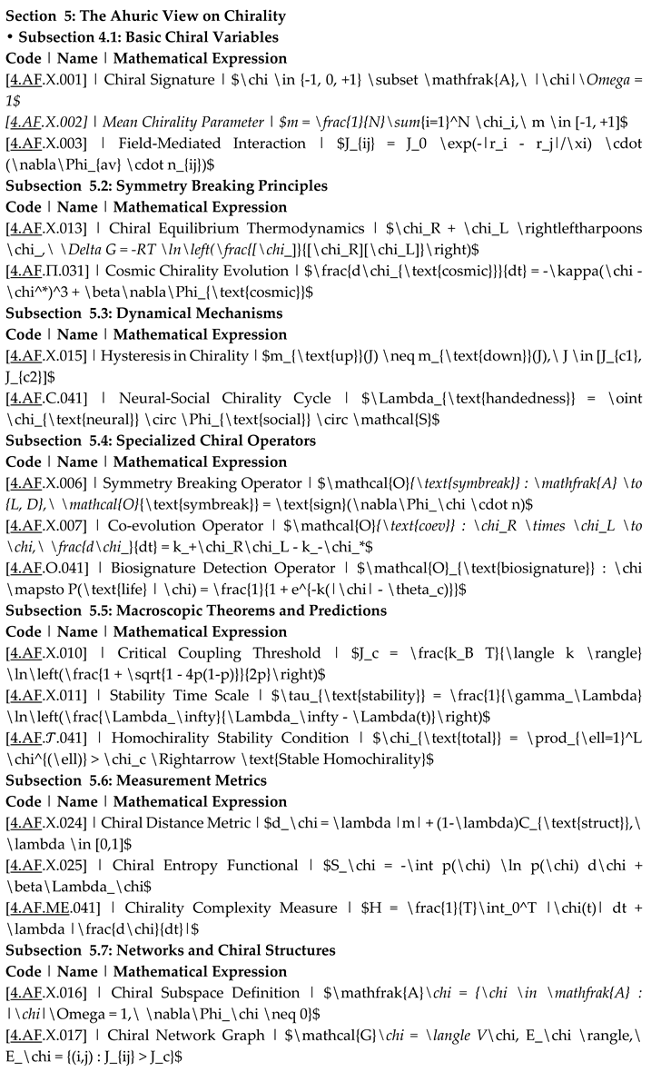
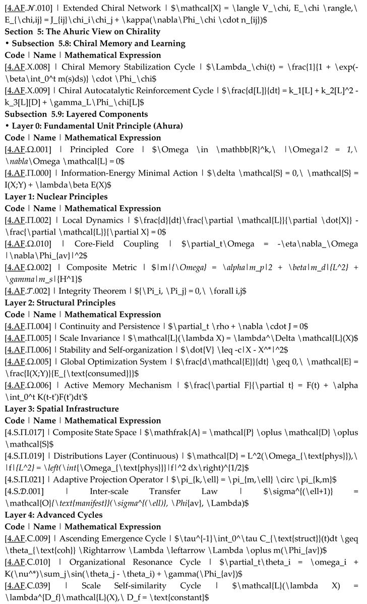
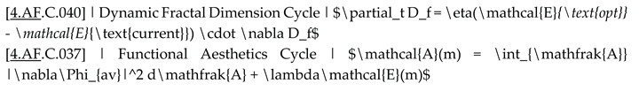
References
- Meskers, S. C. J. (2022). Consequences of chirality on the response of materials. Materials Advances, 3(5), 2324–2336. [CrossRef]
- Gasser, J., & Leutwyler, H. (1984). Chiral Perturbation Theory to One Loop. Annals of Physics, 158(1), 142–210. [CrossRef]
- Sazdjian, H. (2016). Introduction to Chiral Symmetry in QCD. arXiv:1602.03648.
- Ananthanarayan, B., Khan, M. S. A., & Wyler, D. (2023). Reflections on Effective Chiral Theories of the Standard Model. arXiv:2305.10284.
- Thomas, A. W. (2025). Reflections on Chiral Symmetry within QCD. Symmetry, 17(4), 512. [CrossRef]
- Frolov, V. P., Kubizňák, D., & Krtouš, P. (2023). Chiral anomalies in black hole spacetimes. Physical Review D, 107(4), 045009. https://arxiv.org/abs/2212.11320.
- Singh, D. (2004). Neutrino helicity and chirality transitions in Schwarzschild spacetime. arXiv:gr-qc/0401044.
- Campante, T. L., Lund, M. N., Kuszlewicz, J. S., et al. (2016). Spin-orbit alignment of exoplanet systems: ensemble analysis using asteroseismology. arXiv:1601.06052.
- Capozziello, S., & Lattanzi, A. (2005). Spiral Galaxies as Enantiomers: Chirality, an Underlying Feature in Chemistry and Astrophysics. arXiv:astro-ph/0509316.
- Basiri A, Chen X, Bai J, Amrollahi P, Carpenter J, Holman Z, Wang C, Yao Y. Nature-inspired chiral metasurfaces for circular polarization detection and full-Stokes polarimetric measurements. Light: Science & Applications. 2019;8(1):78. [CrossRef]
- Kawamura, H. (2001). Chirality in spin glasses. Journal of the Physical Society of Japan, 70(Suppl. A), 1–14.
- Blackmond, D. G. (2010). The origin of biological homochirality. Cold Spring Harbor Perspectives in Biology, 2(5), a002147. [CrossRef]
- Bonner, W. A. (1991). The origin and amplification of biomolecular chirality. Origins of Life and Evolution of the Biosphere, 21(2), 59–111. [CrossRef]
- Barron, L. D. (2008). Chirality and life. Space Science Reviews, 135(1–4), 187–201.
- Sato, I., et al. (2021). Enzymatic activity in homochiral environments. Chemical Communications, 57(12), 1454–1467.
- Glavin, D. P., Dworkin, J. P., & Lauretta, D. S. (2023). The search for chiral asymmetry as a potential biosignature in our solar system. Chemical Reviews, 123(8), 4669–4702. [CrossRef]
- Bailey, J., et al. (1998). Circular polarization in star-forming regions: implications for biomolecular homochirality. Science, 281(5377), 672–674.
- Yamagata, Y. (1966). A hypothesis for the asymmetric appearance of biomolecules on earth. Journal of Theoretical Biology, 11(3), 495–498.
- Soai, K., et al. (1995). Asymmetric autocatalysis and amplification of enantiomeric excess of a chiral molecule. Nature, 378(6559), 767–768.
- Hein, J. E., & Blackmond, D. G. (2012). On the origin of single chirality of amino acids and sugars in biogenesis. Accounts of Chemical Research, 45(12), 2045–2054.
- Naaman, R., & Waldeck, D. H. (2022). Chiral-induced spin selectivity and the emergence of spin-based biology. Annual Review of Biophysics, 51, 99–114. [CrossRef]
- Theiler, J. P., Graf, J., & Wegner, D. (2025). Non-Hermitian exchange as the origin of chirality-induced spin selectivity. arXiv:2505.06173.
- Blohm I, Miranda S, Ho SY, Leimeister JM. Next-generation IS research methods – towards a better understanding of complex and dynamic phenomena … and Generative AI as the elephant in the room. J Inf Technol. 2025;40(2):102-121. alexandria.unisg.ch+2journals.sagepub.com+2. [CrossRef]
- Bhandari, M., & Reddiboina, M. (2019). Augmented intelligence: A synergy between man and the machine. Indian Journal of Urology, 35(2), 89–91. [CrossRef]
- Schröder, A., Constantiou, I., Tuunainen, V. K., & Austin, R. D. (2022). Human–AI collaboration: Coordinating automation and augmentation tasks in a digital service company. In Proceedings of the 55th Hawaii International Conference on System Sciences (pp. 206–215). [CrossRef]
- Kong, L., Zhang, J., & Li, W. (2025). Examining human–AI collaboration in hybrid intelligence learning environments: Insights from the synergy degree model. Humanities and Social Sciences Communications, 12(1), 5097. [CrossRef]
- Schwab, I. R. (2018). The evolution of eyes: major steps (The Keeler Lecture 2017). Eye, 32, 302–313.
- Nilsson, D. E., & Pelger, S. (1994). A pessimistic estimate of the time required for an eye to evolve. Proceedings of the Royal Society B, 256(1345), 53–58.
- Ogura, A., Yoshida, M. A., & Kito, K. (2004). The eye of the cephalopod: a molecular biological approach. Comparative Biochemistry and Physiology Part B, 139(4), 621–626.
- Ashtekar, A., & Singh, P. (2011). Loop Quantum Cosmology: A Status Report. Classical and Quantum Gravity, 28(21), 213001. [CrossRef]
- Borde, A., Guth, A. H., & Vilenkin, A. (2003). Inflationary spacetimes are not past-complete. Physical Review Letters, 90(15), 151301. [CrossRef]
- Guth, A. H., & Nomura, Y. (2021). What can the multiverse tell us about the measure problem? JCAP, 2021(10), 024. [CrossRef]
- Planck Collaboration. (2020). Planck 2018 results. VII. Isotropy and Statistics of the CMB. Astronomy & Astrophysics, 641, A7. aanda.org+1. [CrossRef]
- Guth, A. H. (1981). Inflationary universe: A possible solution to the horizon and flatness problems. Physical Review D, 23(2), 347–356. [CrossRef]
- Mukhanov, V. F., & Chibisov, G. V. (1981). Quantum fluctuations and a nonsingular universe. JETP Letters, 33, 532–535.
- Guth, A. H., & Pi, S.-Y. (1982). Fluctuations in the new inflationary universe. Physical Review Letters, 49(15), 1110–1113. [CrossRef]
- Peebles, P. J. E. (1980). The Large-Scale Structure of the Universe. Princeton University Press.
- Springel, V., et al. (2005). Simulations of the formation, evolution and clustering of galaxies and quasars. Nature, 435(7042), 629–636. [CrossRef]
- Weinberg, S. (1989). The cosmological constant problem. Reviews of Modern Physics, 61(1), 1–23. [CrossRef]
- Susskind, L. (2003). The anthropic landscape of string theory. arXiv:hep-th/0302219.
- Martínez, M., & Zanolin, M. (2024). Is the Fine-Tuning Evidence for a Multiverse? Synthese. [CrossRef]
- Kauffman, S. (2022). The Anthropic Principle Is Testable and Appears Weak. arXiv:2205.12896.
- Cosmological Fine-Tuning and Life-Permitting Intervals. (2024). arXiv:2401.04190.
- Weinberg, D. H., & White, M. (2023). “28. Dark Energy,” in Review of Particle Physics (PTEP 2022, 083C01; 2023 update). Particle Data Group.
- Quantum Gravity. (2024). Stanford Encyclopedia of Philosophy (Fall 2024 Edition).
- Singh, T. P. (2024). Classical and quantum: a conflict of interest. arXiv preprint.
- Gershon, T., & Nir, Y. (2023). “CP Violation in the Quark Sector.” In Review of Particle Physics, Particle Data Group.
- LHCb Collaboration. (2025). Observation of charge–parity symmetry breaking in baryon decays. Nature. (25 March 2025).
- Croon, D., Gonzalo, T. E., Graf, L., Košnik, N., & White, G. (2019). GUT Physics in the era of the LHC. arXiv:1903.04977.
- Sall Embien, Q., Raynal, M., Crassous, J., … (2022). Possible chemical and physical scenarios towards biological homochirality. Chemical Society Reviews, 51(10), 4025-4044. [CrossRef]
- Smith, J. M., & Szathmáry, E. (2020). The Origins of Life: From the Birth of Life to the Origin of Language (Revised ed.). Oxford University Press.
- Lane, N. (2015). The Vital Question: Energy, Evolution, and the Origins of Complex Life. W. W. Norton & Company.
- Blackmond, D. G. (2019). The Origin of Biological Homochirality. Cold Spring Harbor Perspectives in Biology, 11(3), a032540. [CrossRef]
- Lehn, J.-M. (2022). Perspectives in Chemistry – Steps Towards Complex Matter. Angewandte Chemie International Edition, 61(14), e202200040. [CrossRef]
- Goyal, P., Li, Y., & Nguyen, H. D. (2024). Thermodynamic Control of Molecular Self-Assembly: From Supramolecular Chemistry to Biological Systems. Chemical Reviews, 124(3), 1557–1590. [CrossRef]
- Whitesides, G. M., & Grzybowski, B. (2002). Self-Assembly at All Scales. Science, 295(5564), 2418–2421. [CrossRef]
- McShea, D. W., & Brandon, R. N. (2023). Biology’s First Law: The Tendency for Diversity and Complexity to Increase in Evolutionary Systems. Oxford University Press.
- Lane, N. (2022). Transformer: The Deep Chemistry of Life and Death. W. W. Norton & Company.
- Lynch, M. (2023). The Origins of Cellular Complexity. Proceedings of the National Academy of Sciences, 120(9), e2218930120. [CrossRef]
- Tononi, G., Boly, M., Massimini, M., & Koch, C. (2023). Integrated Information Theory: From Consciousness to its Physical Substrate. Nature Reviews Neuroscience, 24(5), 300–317. [CrossRef]
- Dehaene, S. (2024). Consciousness and the Brain: A Decade of Global Workspace Research. Trends in Cognitive Sciences, 28(1), 12–25. [CrossRef]
- Seth, A. K. (2021). Being You: A New Science of Consciousness. Faber & Faber.
- Pastor-Satorras R, Castellano C, Van Mieghem P, Vespignani A. Epidemic processes in complex networks. Rev Mod Phys. 2015;87(3):925-979. [CrossRef]
- Li, C., Wang, J., & Yu, H. (2023). Modeling and prediction of information diffusion in complex social networks. Information Sciences, 623, 102–121. [CrossRef]
- Holme, P. (2024). Temporal Network Theory: Dynamics, Spreading, and Control. Oxford University Press.
- Todorov, E., & Li, W. (2023). Optimal control and estimation in robotics and autonomous systems. Annual Review of Control, Robotics, and Autonomous Systems, 6, 1–25. [CrossRef]
Disclaimer/Publisher’s Note: The statements, opinions and data contained in all publications are solely those of the individual author(s) and contributor(s) and not of MDPI and/or the editor(s). MDPI and/or the editor(s) disclaim responsibility for any injury to people or property resulting from any ideas, methods, instructions or products referred to in the content. |
© 2025 by the authors. Licensee MDPI, Basel, Switzerland. This article is an open access article distributed under the terms and conditions of the Creative Commons Attribution (CC BY) license (http://creativecommons.org/licenses/by/4.0/).
Copyright: This open access article is published under a Creative Commons CC BY 4.0 license, which permit the free download, distribution, and reuse, provided that the author and preprint are cited in any reuse.


