Submitted:
07 November 2025
Posted:
07 November 2025
You are already at the latest version
Abstract
We investigate time-resolved wave-packet transport in monolayer graphene patterned with asymmetric arrays of circular electrostatic scatterers. Using the Dirac continuum model with a split-operator scheme, we track how transmission evolves with scatterer radius and polarity sequence. To this end, we consider three potential configurations (Samples 1–3). The results reveal a geometry-controlled crossover from near-ballistic propagation at small radii to interference-dominated backscattering at large radii. Sample 1, where the potential exhibit two parallel lines of circles, each line sharing the same potential sign, preserves the highest transmission. Conversely, in Sample 3, where potential signs are intercalated between circles of the same line, the dwell time increases, which produces stronger confinement. As the radius increases, pronounced temporal oscillations emerge due to repeated internal reflections (similar to Fabry–Pérot), and the radius dependence of the saturated transmission probability exhibits anti-resonant dips that are tunable by geometry and potential magnitude. These behaviors establish simple design rules for graphene nanodevices: small-radius Sample 1 for high-throughput transport, Sample 2 (with inverted potential signs as compared to Sample 1) for broadband suppression, and Sample 3 for finely tunable, interference-based confinement.
Keywords:
graphene
; wave-packet
; Gaussian
; propagation
; Dirac equation
; split-operator scheme
; electrostatic scatterers
; potential barrier
; potential well
; asymmetry
; transmission probability
1. Introduction
Graphene, the first isolated two-dimensional (2D) material [1], continues to attract great attention due to its outstanding electronic properties [2,3]. Its linear gapless dispersion near the Dirac points makes charge carriers behave as massless Dirac fermions [4,5], resulting in ultra-high mobility and unconventional quantum transport compared to conventional semiconductors [6,7].
A hallmark of this relativistic behavior is the Klein paradox, where carriers tunnel almost perfectly through electrostatic barriers. This effect, while fundamental, poses challenges for confinement in graphene-based devices. Recent experiments have confirmed its strong angle-dependent nature [8], highlighting the importance of theoretical tools such as wave-packet dynamics [9,10,11]. Suppressing or controlling this robust tunneling is essential for developing functional nanodevices [12,13,14].
Artificial potential landscapes (APLs) [15] offer a practical route to modulate carrier flow. Previous studies examined wave-packet propagation under magnetic fields [16,17,18] and through scattering potentials [19,20,21,22] using established approaches, including trajectory simulations [23,24] and time-dependent Dirac equation solvers [25,26,27,28]. APLs can generate localized electron-hole puddles [29,30], and while random disorder has been widely studied [31,32], systematic analysis of ordered polarity sequences in minimal scattering arrays remains limited. Geometry-based control of pseudospin and chirality-dependent tunneling [33,34] is therefore a promising direction, supported by recent advances in graphene device fabrication [35,36,37].
In this work, we numerically investigate wave-packet dynamics in monolayer graphene under three polarity-dependent APL configurations. The calculations are performed out within the Dirac continuum model, and time propagation is carried out using the split operator technique [38,39]. We analyze how potential scatterer arrangement, size, and magnitude govern electronic transmission. Our results demonstrate that subtle spatial-polarity variations strongly influence quantum interference and backscattering, providing design principles for tunable electron transport in future graphene nanodevices.
2. System Description and Theoretical Framework
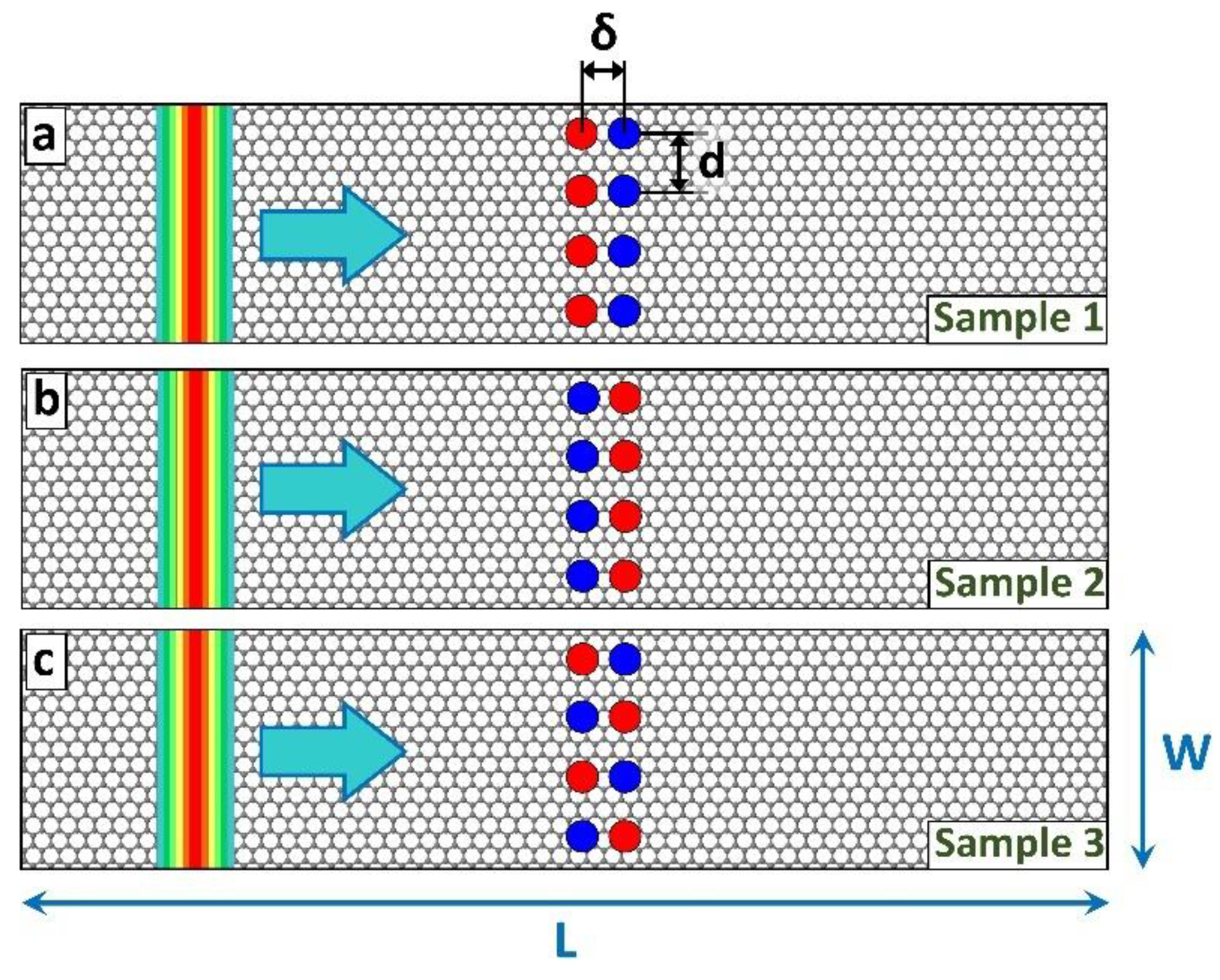
A schematic representation of the model system is shown in Fig. 1. It consists of a monolayer pristine graphene sheet with dimensions of L = 1024 nm (length) and W = 128 nm (width), into which circular electrostatic scatterers are embedded in two vertical lines. Three configurations are considered: (a) Sample 1 features a set of circular potential barriers and circular potential wells; (b) Sample 2 is similar to Sample 1, but with inverted potential signs, i.e., the propagating wave packet will meet first a set of circular potential wells and then a set of potential barriers; (c) Sample 3 implements potential scatterers in an asymmetric way: in the first line (top), one places a potential barrier and then a potential well (from left to right), while in the next line these potential barrier and well flip sides, so that first a potential well is placed and then a potential barriers is placed.
The center-to-center spacing between adjacent potential scatterers in the x and y direction is set to δ=d=32 nm. To investigate the influence of obstacle size on wave packet dynamics, six representative barrier and well radii, R = 5, 7, 9, 11, 13, and 15 nm, are considered. Furthermore, to examine the effect of the potential scatterers, we consider a wide range of scattering potential heights, varying the magnitude from 20 meV up to 300 meV.
Figure 1.
Schematic representation of wave packet propagation (indicated by the rainbow-colored wave front and cyan arrow) across a monolayer graphene sheet subjected to artificial potential configurations. Red (blue) circles represent potential barriers (wells).
Figure 1.
Schematic representation of wave packet propagation (indicated by the rainbow-colored wave front and cyan arrow) across a monolayer graphene sheet subjected to artificial potential configurations. Red (blue) circles represent potential barriers (wells).
The wave packet is modeled as a Gaussian wave front characterized by its energy E and width ax. Specifically, the initial wave packet is a Gaussian function constant in the y-direction, with a finite width in the x-direction, and is expressed as:
where N is the normalization constant and k is the wave vector, which is related to the wave packet energy E by k=E/ℏvF, where vF being the Fermi velocity in graphene. The pseudo-spinor (1 1)T is selected to ensure propagation along the x-direction, with ⟨σx⟩=1 and ⟨σy⟩=⟨σz⟩=0. All simulations in this study assumed a wave packet with an energy and width of 100 meV and 10 nm, respectively, without loss of generality: due to the linear dispersion of the system, it is rather the comparison between potential barrier and wave packet energy, and not its energy itself, which has a significant influence on the scattering results.
The wave packet propagation is governed by the time-evolution operator applied to the initial wave packet:
where H is the Hamiltonian for relativistic electrons in graphene around Dirac cone (which is a good approximation for low energy states):
with representing the Pauli matrices, I being the 2×2 identity matrix, and V(x, y) denoting the scalar potential. The wave functions are written as pseudo-spinors Ψ = (ΨA ΨB)T, where ΨA (ΨB) corresponds to probabilities of the electron being in sublattices A (B).
In order to simplify the calculations, the split-operator technique [38] is employed:
where terms of order O(Δt3) and higher are neglected by assuming small time steps Δt. This approach enables efficient multiplication in real and reciprocal spaces, avoiding the explicit differentiation of the momentum operator by utilizing the Fourier transform and expressing . Furthermore, the exponentials involving Pauli matrices can be exactly reformulated as matrices [17]. Simulations were performed with a time step of Δt = 0.1 fs, and the probabilities of finding the electron before, inside, and after the scattering region are computed. The latter was interpreted as the transmission probability (P) through the scattering region. To avoid numerical artifacts associated with periodic boundary conditions, we employed a sufficiently large computational grid of 1024 nm × 128 nm, while the scattering centers were confined to a smaller scattering region (42 nm × 128 nm for R= 5 nm, or 62 nm × 128 nm for R= 15 nm) around the x = 0 axis. This ensured accurate evaluation of the transmission and reflection probabilities, by allowing one to collect data on transmission probabilities long before the wave packet reaches the edges of the computational box. As mentioned above, all simulations were conducted at a wave packet energy of E=100 meV. This done in order to ensure that the results remain within the range of applicability of the Dirac continuum model, i.e., around Dirac cone (low energy state).
3. Results and Discussion
Figure 2 presents the time evolution of the transmission probability P for the three lattice con-figurations (Samples 1–3) assuming two values of scatterer radii, i.e., R=5 nm (smallest scatterer) and R=15 nm (largest scatterer). For R=5 nm the packet exits the scattering region rapidly and the transmission stabilizes by t≈400 fs in all samples. The Sample 1 yields the largest P, evidencing weak scattering and minimal back-reflection; transmission remains nearly perfect (i.e., ~1.0) across the whole ∣V0∣ range, reflecting the dominance of Klein tunneling for narrow barriers. Introducing the configurations of Samples 2 and 3 lowers the long-time transmission and slows its approach to the plateau, indicating stronger multiple scattering and partial confinement inside the potential land-scape. Among these, Sample 3 consistently gives the smallest final P, i.e., the strongest confinement for small scatterers. The slight decrease of P with increasing ∣V0∣ in Samples 2–3 suggests weak perturbation channels opened by the non-staggered alignments.
The dependence on barrier height is also configuration-sensitive. For R=5 nm, P decreases with increasing ∣V0∣ in Samples 1 and 3, reaching about 0.91 and 0.65 at ∣V0∣=300 meV, respectively. In Sample 2, P likewise drops as ∣V0∣ increases up to ∼220 meV (to ∼0.78), but then recovers to ∼0.86 at ∣V0∣=300 meV. The reason for this increase in P at higher potential magnitudes is the emergence of interference-assisted, quasi-resonant transmission of Dirac carriers: as ∣V0∣ grows, the phase accumulated across successive barriers satisfies constructive-interference conditions and, for narrow scatterers, the effective barrier becomes more transparent to near-normal components of the packet, partially restoring forward transmission despite the larger potential.
When the radius is increased to R=15 nm, transmission drops markedly in all samples and pronounced temporal oscillations appear between ∼150-400 fs. These oscillations arise from repeated internal reflections within the extended scattering region, an analogue of Fabry-Pérot resonances, and they are strongest in all Samples, where the geometry increases dwell time and enhances back-reflection. At high ∣V0∣, the transmission typically stabilizes between ∼0.6 and 0.8; the broader footprint increases the backscattering and thereby suppresses the effectiveness of Klein tunneling. The interference pattern depends sensitively on the polarity sequence, with the mixed arrangement of Sample 3 exhibiting the lowest transmission and the most complex oscillatory behavior, under-scoring its role as an efficient geometry for transport modulation. Although Figure 2 displays repre-sentative traces for R=5 and 15 nm, the complete set of time-dependent transmission curves for R=5, 7, 9, 11, 13, and 15 nm is provided in Supplementary Figure S1; these data confirm the same geometry-dependent trends and show the progressive emergence of oscillations as R increases. To facilitate interpretation, the Supplementary Material also includes wave-packet propagation animations at ∣V0∣=260 meV for R=5 and 15 nm, which helps to visualize the contrast between rapid, single-pass transmission and prolonged dwell with multiple internal reflections that underlie the oscillatory behavior discussed above.
Overall, Figure 2 demonstrates that both the spatial arrangement and the size of the electro-static scatterers control the balance between transmission and confinement: small, symmetric arrays favor smooth passage, while larger and more complex lattices promote multiple scattering, transient localization, and reduced transmission. Thus, for the smallest scatterers (R=5 nm) the strongest confinement occurs in Sample 3, whereas for the largest scatterers (R=15 nm) the strongest confinement is observed in Samples 2 and 3.
Figure 3 clarifies the origin of the oscillations observed in Figure 2 for the large-radius case (R=15 nm) by showing a representative time trace obtained at a single barrier height, ∣V0∣=260 meV. After the packet arrives at the scattering centers region (at t≈100 fs), the probability inside the scattering region (red) does not decay monotonically but exhibits a sequence of revivals. These arise from recurrent internal reflections between adjacent potential rows: each bounce partitions the packet into backward and forward components, producing secondary rises in the reflected probability (black) and a step-like, oscillatory growth of the transmission probability (blue). This behavior is a time-domain analogue of a Fabry–Pérot interferometer, where the phase accumulated along different paths alternately enhances and suppresses the forward flux. Since a larger radius increases both the scattering and the effective path length, the dwell time is longer and the interference contrast is stronger for larger scatterers, which explains why the oscillations are pronounced for R=15 nm but weak for R=5 nm.
The sample-to-sample differences follow naturally: in Samples 2 and 3 the red curve remains elevated for longer and shows multiple peaks, the blue curve rises more slowly with larger undulations, and the black curve develops secondary humps from delayed backscattering. In contrast, in Sample 1 the red probability decays more quickly and the blue probability approaches its plateau smoothly. Although Figure 3 is presented for ∣V0∣=260 meV, it serves as a clear example of the geometry-induced multiple scattering and phase-coherent interference that generate the time-resolved transmission modulations seen across the R=15 nm panels of Figure 2.
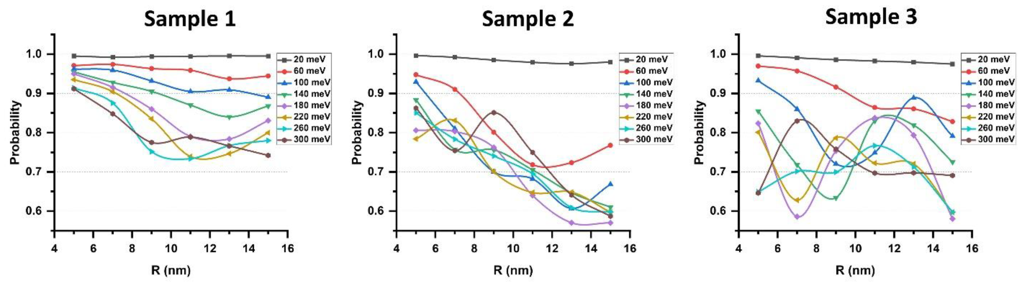
Figure 4 summarizes the saturated values of the P as a function of scatterer radius and makes clear how geometry governs the crossover from nearly ballistic transport to interference-dominated backscattering. For small radii and low barrier (well) potential height (depth), P is close to unity in all configurations, consistent with weak momentum transfer and the prevalence of Klein tunneling for narrow barriers.
As R increases, the dwell time grows, and the P becomes strongly configuration dependent. In Sample 1 the curves decrease almost monotonically with R, indicating a progressive but relatively simple suppression of forward flux. In Sample 2, the decline is steeper and develops broad minima around R∼13–15 nm, most pronounced at higher ∣V0∣ (≈140–300 meV); notably, at ∣V0∣=180 meV the transmission reaches its lowest value P=0.57 at both R=13 and 15 nm. This indicates the accumulation of the destructive phase in successive rows and the onset of quasi-resonant backscattering. Sample 3 exhibits the most dramatic non-monotonicity, with alternating peaks and deep anti-resonant dips whose positions shift with ∣V0∣; specifically, at ∣V0∣=180 meV the minimum transmission is P=0.58 occurring at R=7 nm and again at R=15 nm. This oscillatory structure mirrors the time-domain behavior seen in Figure 2 and the partition dynamics in Figure 3: larger radii promote repeated internal reflections and phase-coherent interference, so small changes in R and ∣V0∣ toggle between constructive and destructive transmission channels. Practically, these trends suggest complementary operating regimes: Sample 1 at small R for high-throughput transport, Sample 2 at large R for broadband suppression, and Sample 3 for finely tunable filtering where targeted radii and potentials can be chosen to exploit the deepest interference-induced transmission minima.
4. Conclusions
Time-resolved and radius-dependent simulations demonstrate a geometry-driven crossover in graphene from nearly ballistic transport to interference-dominated backscattering. For small scatterers (R=5 nm), transmission saturates rapidly and remains highest for Sample 1, while Samples 2 and 3 reduce the transmission plateau and slow its approach; among them, Sample 3 provides the strongest confinement, lowering the saturated transmission to ∼0.65 at ∣V0∣=300 meV. Increasing the radius to R=15 nm suppresses transmission in all geometries and introduces pronounced temporal modulations between ∼150-400 fs; decomposition of the probability at ∣V0∣=260 meV confirms that these oscillations arise from recurrent internal reflections and phase-coherent partitioning within the barrier array.
Mapping the saturated transmission versus radius consolidates the design rules discussed here. Sample 1 decreases almost monotonically with R, indicating progressive, yet trivial, suppression of forward flux. Sample 2 develops broad minima around R∼13-15 nm, with a lowest P=0.57 at R=13 and 15 nm for ∣V0∣=180 meV. Sample 3 exhibits the deepest, most tunable anti-resonant dips, reaching P=0.58 at R=7 and 15 nm for ∣V0∣=180 meV. These results identify clear operating regimes: small-R Sample 1 for high-throughput transport, large-R Sample 2 for broadband suppression, and Sample 3 for finely tunable, interference-based confinement.
Supplementary Materials
The following supporting information can be downloaded at the website of this paper posted on Preprints.org.
References
- Novoselov, K.S.; Geim, A.K.; Morozov, S.V.; et al. Electric field effect in atomically thin carbon films. Science 2004, 306, 666–669. [Google Scholar] [CrossRef]
- Geim, A.K.; Novoselov, K.S. The rise of graphene. Nat. Mater. 2007, 6, 169–175. [Google Scholar] [CrossRef] [PubMed]
- Geim, A.K. Graphene: Status and prospects. Science 2009, 324, 1530–1534. [Google Scholar] [CrossRef] [PubMed]
- Castro Neto, A.H.; et al., A.K. The electronic properties of graphene. Rev. Mod. Phys. 2009, 81, 109–162.
- Novoselov, K.S.; et al. A roadmap for graphene. Nature 2012, 490, 192–200.
- Wang, S.; et al. Quantum transport in Dirac and Weyl semimetals: a review. Adv. Phys. X 2017, 2, 518–544. [Google Scholar] [CrossRef]
- Zivieri, R.; Lumetti, S.; Létang, J. High-Mobility Topological Semimetals as Novel Materials for Huge Magnetoresistance Effect and New Type of Quantum Hall Effect. Materials 2023, 16, 7579. [Google Scholar] [CrossRef]
- Zhang, Z.; et al. Angular-dependent Klein tunneling in photonic graphene. Phys. Rev. Lett. 2022, 129, 233901. [Google Scholar] [CrossRef]
- Sundaram, G.; Niu, Q. Wave-packet dynamics in slowly perturbed crystals: Gradient corrections and Berry-phase effects. Phys. Rev. B 1999, 59, 14915–14925. [Google Scholar] [CrossRef]
- Lapa, M.F.; Hughes, T.L. Semiclassical wave packet dynamics in nonuniform electric fields. Phys. Rev. B 2019, 99, 121111(R). [Google Scholar] [CrossRef]
- Ren, Y.; Sánchez Barrero, M.E. Nonadiabatic Wave-Packet Dynamics: Nonadiabatic Metric, Quantum Geometry, and Analogue Gravity. arXiv preprint arXiv:2509.00166, 2025.
- Walls, J.D.; Hadad, D. Suppressing Klein tunneling in graphene using a one-dimensional array of localized scatterers. Sci. Rep. 2015, 5, 8435. [Google Scholar] [CrossRef] [PubMed]
- Yusupov, J.R.; et al. Driven transparent quantum graphs. Phys. Scr. 2025, 100, 075224. [Google Scholar] [CrossRef]
- Tan, Y.; et al. Graphene Klein tunnel transistors for high speed analog RF applications. Sci. Rep. 2017, 7, 9714. [Google Scholar] [CrossRef]
- Jiang, Q.-D.; et al. Chiral wave-packet scattering in Weyl semimetals. Phys. Rev. B 2016, 93, 195165. [Google Scholar] [CrossRef]
- Romera, E.; de los Santos, F. Revivals, classical periodicity, and zitterbewegung of electron currents in monolayer graphene. Phys. Rev. B 2009, 80, 165416. [Google Scholar] [CrossRef]
- Rakhimov, Kh.; et al. Wavepacket scattering of Dirac and Schrödinger particles on potential and magnetic barriers. J. Phys.: Condens. Matter 2011, 23, 275801. [Google Scholar] [CrossRef]
- Chaves, A.; et al. Wave-packet dynamics and valley filter in strained graphene. Phys. Rev. B 2010, 82, 205430. [Google Scholar] [CrossRef]
- Palpacelli, S.; et al. Klein tunneling in the presence of random impurities. Int. J. Mod. Phys. C 2012, 23, 1250080. [Google Scholar] [CrossRef]
- Egger, R.; et al. (Eds.) Low-Dimensional Functional Materials; Springer: Berlin, Germany, 2013; p. 119. [Google Scholar]
- Suleimanov, M.; et al. Wave-packet dynamics in monolayer graphene with periodic scattering potentials. Physica B 2025, 714, 417484. [Google Scholar] [CrossRef]
- Rakhimov, Kh.; et al. Wave-packet rectification in graphene with alternating circular electrostatic potential barriers. J. Appl. Phys. 2025, 137, 144302. [Google Scholar] [CrossRef]
- Paredes-Rocha, E.; et al. Gradient-index electron optics in graphene p −n junctions. Phys. Rev. B 2021, 103, 045404. [Google Scholar] [CrossRef]
- Chen, Sh.; et al. Electron optics with pn junctions in ballistic graphene. Science 2016, 353, 1522–1525. [Google Scholar] [CrossRef] [PubMed]
- Braun, J.W.; Su, Q.; Grobe, R. Numerical approach to solve the time-dependent Dirac equation. Phys. Rev. A 1999, 59, 604–612. [Google Scholar] [CrossRef]
- Fillion-Gourdeau, F.; Lorin, E.; Bandrauk, A.D. Numerical solution of the time-dependent Dirac equation in coordinate space without fermion-doubling. Comput. Phys. Commun. 2012, 183, 1403–1415. [Google Scholar] [CrossRef]
- Akramov, M.E.; et al. Discrete sine-Gordon equation on metric graphs: A simple model for Josephson junction networks. Phys. Scr. 2023, 98, 115238. [Google Scholar] [CrossRef]
- Akramov, M.E.; et al. Transparent boundary conditions for the nonlocal nonlinear Schrödinger equation: A model for reflectionless propagation of PT-symmetric solitons. Phys. Lett. A 2023, 459, 128611. [Google Scholar] [CrossRef]
- Martin, J.; et al. Observation of electron-hole puddles in graphene using a scanning single-electron transistor. Nat. Phys. 2008, 4, 144–148. [Google Scholar] [CrossRef]
- Zhang, Y.; et al. Origin of spatial charge inhomogeneity in graphene. Nat. Phys. 2009, 5, 722–726. [Google Scholar] [CrossRef]
- Mucciolo, E.R.; Lewenkopf, C.H. Disorder and electronic transport in graphene. J. Phys.: Condens. Matter 2010, 22, 273201. [Google Scholar] [CrossRef]
- Zhao, P.-L.; et al. Fingerprints of disorder source in graphene. Phys. Rev. B 2015, 92, 045437. [Google Scholar] [CrossRef]
- Rickhaus, P.; et al. Gate tuneable beamsplitter in ballistic graphene. Appl. Phys. Lett. 2015, 107, 251901. [Google Scholar] [CrossRef]
- Liu, J.-L.; Ye, W.-M.; Zhang, S. Pseudospin-induced chirality with staggered optical graphene. Light Sci. Appl. 2016, 5, e16094. [Google Scholar] [CrossRef]
- Han, C.-D.; Xu, H.-Y.; Lai, Y.-C. Pseudospin modulation in coupled graphene systems. Phys. Rev. Research 2020, 2, 033406. [Google Scholar] [CrossRef]
- Kammarchedu, V.; et al. Recent advances in graphene-based electroanalytical devices for healthcare applications. Nanoscale 2024, 16, 12857–12865. [Google Scholar] [CrossRef]
- Smith, A.D.; et al. Large scale integration of graphene transistors for potential applications in the back end of the line. Solid-State Electron. 2015, 108, 61–66. [Google Scholar] [CrossRef]
- Chaves, A.; et al. The split-operator technique for the study of spinorial wavepacket dynamics. Commun. Comput. Phys. 2015, 17, 850–872. [Google Scholar] [CrossRef]
- Degani, M.H.; Leburton, J.P. Single-electron states and conductance in lateral-surface superlattices. Phys. Rev. B 1991, 44, 10901–10909. [Google Scholar] [CrossRef] [PubMed]
Figure 2.
Transmission probability (P) as a function of time for three distinct scattering configurations (Samples 1–3) under various potential magnitudes (∣V0∣). The influence of the scatterer radius (R) is shown by separating the data into the upper row (R = 5 nm) and the lower row (R = 15 nm).
Figure 2.
Transmission probability (P) as a function of time for three distinct scattering configurations (Samples 1–3) under various potential magnitudes (∣V0∣). The influence of the scatterer radius (R) is shown by separating the data into the upper row (R = 5 nm) and the lower row (R = 15 nm).
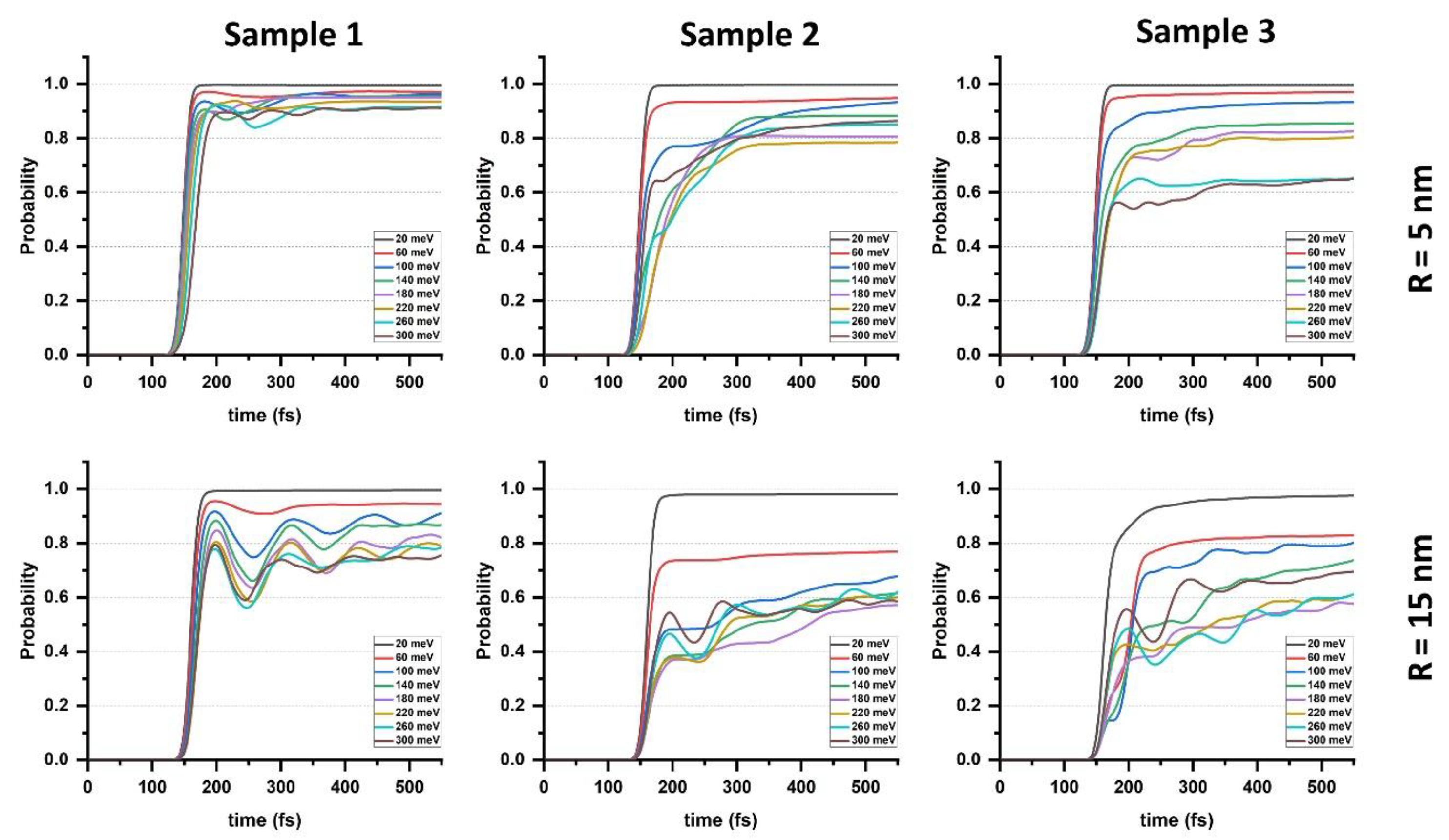
Figure 3.
Time evolution of the wave-packet probability before (black), inside (red), and after (blue) the scattering region for Samples 1–3 at ∣V0∣=260 meV and radii R=5 nm and R=15 nm. For small scatterers, transmission occurs rapidly with minimal reflection, while for large scatterers pronounced oscillations arise from multiple internal reflections and interference, explaining the time-domain modulations observed in Figure 2.
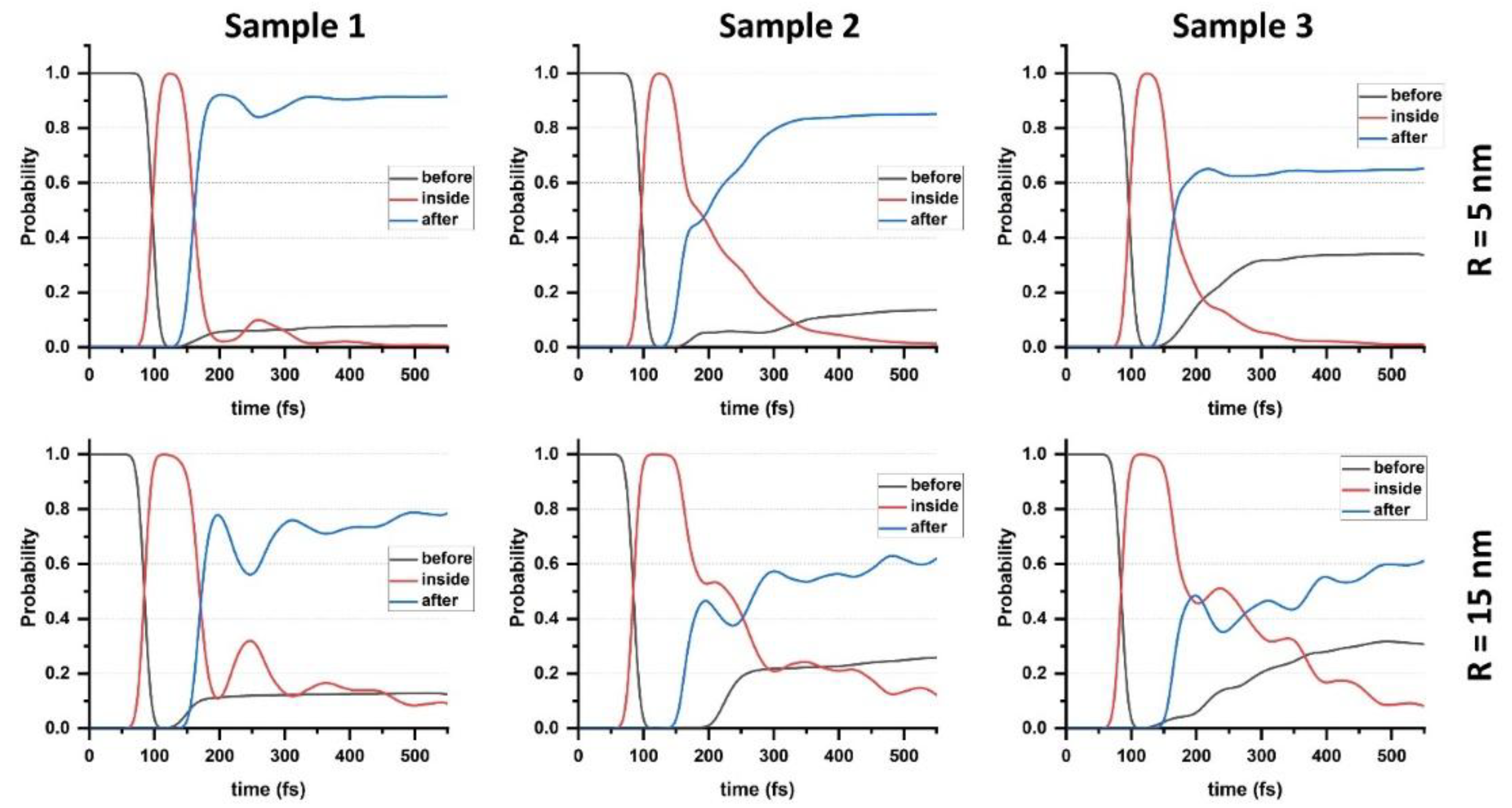
Figure 4.
Saturated P as a function of radii of the scatterers (R=5-15 nm) for different values of potential height/depth. The data highlights the transition from near-perfect transmission at small R to strong, non-monotonic backscattering at large R.
Figure 4.
Saturated P as a function of radii of the scatterers (R=5-15 nm) for different values of potential height/depth. The data highlights the transition from near-perfect transmission at small R to strong, non-monotonic backscattering at large R.
Disclaimer/Publisher’s Note: The statements, opinions and data contained in all publications are solely those of the individual author(s) and contributor(s) and not of MDPI and/or the editor(s). MDPI and/or the editor(s) disclaim responsibility for any injury to people or property resulting from any ideas, methods, instructions or products referred to in the content. |
© 2025 by the authors. Licensee MDPI, Basel, Switzerland. This article is an open access article distributed under the terms and conditions of the Creative Commons Attribution (CC BY) license (http://creativecommons.org/licenses/by/4.0/).
Copyright: This open access article is published under a Creative Commons CC BY 4.0 license, which permit the free download, distribution, and reuse, provided that the author and preprint are cited in any reuse.


