
Submitted:
05 November 2025
Posted:
06 November 2025
You are already at the latest version
Abstract
Remaining Useful Life prediction for rotating machinery is severely hindered by the scarcity of full-life data, which limits the efficacy of data-hungry end-to-end models. To address this data-efficiency challenge, this paper proposes a hybrid learning framework. First, a self-supervised health indicator is constructed from raw vibration signals using contrastive learning. The proposed model, trained with a service-time-based loss, learns a robust 1D degradation representation from minimal data. Second, an Unscented Kalman Filter is employed to model the nonlinear trajectory and stochastic fluctuations of the constructed health indicator. The UKF performs stepwise prediction to forecast when the health indicator will cross a predefined failure threshold. The framework is validated on public bearing datasets and a set of spiral bevel gear experiments, simulating a practical scenario by training on a single full-life sample. Results show the CL-based health indicator achieves superior monotonicity (0.716) and correlation (0.911) compared to baselines. The full framework demonstrates the highest prediction accuracy (0.392), validating its effectiveness and robustness for data-efficient prognostics.
Keywords:
Remaining Useful Life
; health indicator
; contrastive learning
; Unscented Kalman Filter
; data-efficient prognostics
I. Introduction
In the operational service of rotating machinery, acquiring sufficient full-life data is often infeasible, leaving only limited datasets available for analysis and model training [1,2,3,4]. Furthermore, the significant variance in the lifespans of individual components means that end-to-end Remaining Useful Life (RUL) prediction models, which are directly supervised by RUL labels, are prone to substantial prediction inaccuracies [5].
An alternative approach is RUL prediction based on a Health Indicator (HI), which aims to transform full-life data into an HI set and subsequently forecast its evolution based on observed changes [6]. The RUL is ultimately determined when the predicted HI trajectory crosses a predefined failure threshold. The construction of a robust HI is the most critical step; an indicator characterized by a distinct degradation trend can significantly enhance the accuracy and reliability of RUL predictions. The procedural framework for HI-based RUL prediction typically involves four steps: (1) constructing the HI for the training data [7]; (2) learning the degradation characteristics and determining the failure threshold from the training HI [8]; (3) constructing the HI for the test data and evaluating its quality [9]; and (4) performing stepwise prediction of the future HI trajectory from a selected starting point, comparing it against the failure threshold to determine the RUL, and evaluating the overall prediction performance [10].
However, this approach faces several challenges. Conventional methods may prove ineffective when a nonlinear relationship exists between the health state of critical rotating machinery components and the various monitored features [11]. Furthermore, in practical applications, the process of labeling full-life data with specific a priori health indicators can introduce human bias, and the resulting degradation trend is highly dependent on the chosen labeling method [12]. Inappropriate labels can lead to irrational degradation patterns, ultimately preventing the HI from accurately reflecting the true health status of the equipment.
To address these issues, this chapter proposes an RUL prediction algorithm specifically designed for scenarios with limited full-life data. The algorithm is composed of two main components: a method for constructing a health indicator from the full-life data of critical rotating machinery components using contrastive learning, and a stepwise prediction method for the health indicator based on the Unscented Kalman Filter [13] (UKF).
The remainder of this paper is organized as follows: Section 2 introduces the Unscented Kalman Filter and proposes a method for its application in stepwise HI prediction for both training and test sets. Section 3 presents the overall RUL prediction algorithm, which includes the HI construction and stepwise prediction modules, and details the experimental settings such as model hyperparameters, evaluation metrics for the HI, and task configurations. Section 4 validates the effectiveness of the proposed method for both HI construction and RUL prediction using two datasets, supported by comparative and ablation studies. Finally, Section 5 summarizes the findings of this chapter.
II. Methodology & System Architecture
The HIs derived from full-life data possess inherent tenability and monotonicity. However, due to the inevitable noise in the data acquisition process, these indicators also exhibit fluctuations. Therefore, the UKF can be employed to both filter the HI and perform its stepwise prediction.
A. Unsented Kalman Filter
The UKF handles nonlinearities effectively through the Unscented Transformation (UT), which circumvents the pitfalls of linearization and better preserves the higher-order statistics of the system state. As the core step of the UKF, the UT propagates a finite number of sample points (sigma points) through the true nonlinear system to accurately capture the mean and covariance of the state distribution.
The evolution of the equipment's true health state over time is described by the process model. We define the state at time t as the true, underlying Health Indicator value, denoted as HIt Its progression from the previous state HIt-1 is modeled as
where represents the nonlinear degradation function that governs the state transition, and is the process noise, assumed to be a zero-mean Gaussian with covariance Q. This noise term accounts for the inherent uncertainties in the degradation process itself.
The observation at time t, denoted as , is the HI value calculated by our contrastive learning model from the raw sensor data. This measured value is a noisy observation of the true state
where the observation function is an identity function, as the constructed is a direct measurement of the system's health state. The term represents the measurement noise, assumed to be a zero-mean Gaussian with covariance R, which captures uncertainties from the sensor measurements and the HI construction process.
Unlike the Extended Kalman Filter's reliance on first-order Taylor series approximations and Jacobian matrix calculations, the UT uses the sigma points to directly propagate the state distribution. The basic procedure is as follows:
Step 1: Assuming the estimated HI and its covariance at step t−1, denoted as and , are known. A set of sigma points are generated based on the previous state estimate and covariance ,
where L is the dimension of the state (in our case, L=1), and λ is a scaling parameter.
Step 2: The sigma points are propagated through the nonlinear degradation function ,
The a priori HI estimate and covariance are then calculated as the weighted sum of the transformed points,
where and are the weights for the mean and covariance, respectively. An additional correction term is introduced at the central sigma point , where is a non-negative weighting parameter used to characterize the distribution properties and to account for higher-order moments of the distribution. For Gaussian distributions, is typically set to 2.
Step 3: When a new measurement (the HI value from the contrastive model) becomes available, the state estimate is corrected. The a priori HI estimate is used to predict the measurement, and the Kalman gain is computed. The final, a posteriori state estimate and its covariance are updated as follows,
where is the innovation covariance matrix. This updated estimate represents the filtered HI value at time t.
B. Stepwise Prediction of HI
The UKF algorithm is applied to the stepwise prediction of the HI to enable both its filtering and effective forecasting. The pseudocode for this UKF-based stepwise HI prediction process is described in Algorithm 1.
| Algorithm 1: Step-by-step HI Prediction Process based on Unscented Kalman Filter |
| Input: HI for the training and test sets. |
| Phase I: Training Set |
| 1. Define the state transition function f(x, t) and the observation function h(x). |
| 2. Initialize the initial state estimate = 0 and the initial covariance matrix P = 0. |
| 3. Determine the turning point t0 and the threshold HImax. |
| 4. for t=1 to t0-1 do |
| 5. Predict the state mean and P according to Eq. (5). |
| 6. Update the state and P according to Eq. (6). |
| 7. end for |
| 8. for t = t0, ..., T do |
| 9. Predict the state mean and P according to Eq. (5). |
| 10. Update the state and P according to Eq. (6). |
| 11. end for |
| 12. Obtain the final predicted HI for the training set and adjust the parameters of the state transition function f(x, t) based on the deviation from the actual HI. |
| Phase II: Test Set (when f(x, t) and h(x) are adjusted) |
| 13. Same as step 2 |
| 14. for t = 1 to task do (task is the last known time point) |
| 15. Predict the state mean and P according to Eq. (5). |
| 16. Update the state and P according to Eq. (7). |
| 17. end for |
| 18. while x < HImax do |
| 19. Predict the state mean and P according to Eq. (5). |
| 20. Update the state and P according to Eq. (7). |
| 21. end while |
| Output: Predicted RUL for the test set. |
Updating the model with real-time observations is a critical aspect of the UKF, enabling the real-time correction of errors and adjustment of the model's output. However, in the context of stepwise HI prediction, particularly during the testing phase, the model must not be exposed to future HI values (i.e., future observations), as this would constitute information leakage. Therefore, to facilitate the update process in the absence of future data, the model is updated using the predicted HI augmented with a random bias.
For the training set, the model has access to all information from the single full-life dataset, including the failure time. First, the failure threshold is defined as the maximum value of the HI observed in this training data. A turning point is then established to partition the data. Prior to this turning point, the model is updated using the actual observed HI values in a filtering process. After the turning point, the model is updated using the predicted HI with a random bias, and this predict-update cycle is iterated until the end of life is reached. Finally, the parameters of the state transition function are adjusted based on the overall prediction performance on the training set.
For the test set, to simulate a practical engineering scenario, the model can only access data up to a specific point in time, as determined by the test task, without any knowledge of the actual failure time. For instance, in a test where 10 hours of data have been collected, the model uses the observed HI values within this 10-hour window for the filtering process. Beyond this point, where no further data is available, the model is updated by iterating the predict-update cycle using the predicted HI with a random bias. The prediction continues until the forecasted HI exceeds the predefined failure threshold, and the time at which this occurs is used to determine the predicted RUL.
Since the HI for a critical rotating machinery component is represented as a one-dimensional vector, the HI value at any given time, HI(t), is a scalar. Consequently, the state estimate x, the covariance matrix P, the process noise covariance Q, and the measurement noise covariance R are all treated as scalar quantities in this application.
In contrast to the end-to-end RUL prediction algorithm, the HI-based RUL prediction algorithm is composed of two primary modules: HI construction and stepwise HI prediction. Consequently, a distinct standardized procedure is required to guide the experimental setup, encompassing model hyperparameters, evaluation metrics, and task configurations. Leveraging the preprocessed data from two independent datasets, an HI-based RUL prediction algorithm is proposed. The framework for this algorithm is illustrated in Figure 1.
C. Hyperparameters of the HI-RUL Prediction Model
By integrating the contrastive learning-based HI construction method with the UKF-based stepwise HI prediction method, an HI-based RUL prediction model is constructed. The architecture of this HI-based RUL prediction model is illustrated in Figure 2. Within this model, the ReLU activation function and Batch Normalization layers, which could otherwise distort the HI's distribution, are omitted. Furthermore, the linear layers of the frequency-domain encoder (FDE) and the time-frequency domain encoder (WICB) are fused, culminating in a single output neuron to produce a one-dimensional contrastive representation. The hyperparameter settings for the HI-based RUL prediction model are detailed in Table 1.
The data preprocessing hyperparameters include the slicing indices for the envelope spectrum and the multipoint optimal minimum entropy deconvolution adjusted [14] (MOMEDA) output. The hyperparameters for the contrastive learning-based HI construction module include the temperature parameter τ for the loss function, the linear layer size of the feature encoders, and the max-pooling stride. In this module, the two linear layers from the frequency-domain and time-frequency-domain encoders are fused into a single linear layer, and activation functions are omitted, ultimately ensuring the dimensionality of the contrastive representation is 1, which meets the requirement for outputting an HI
The hyperparameters for the stepwise HI prediction module include the UKF's scaling parameter α, the secondary parameter κ, the process noise covariance Q, and the measurement noise covariance R. The scaling parameter α controls the spread of the sigma points; it is typically set to a small value to keep the points close to the state mean. A value of 0.1 is chosen, which allows for an accurate approximation of the state mean, though it may underestimate nonlinear effects; subsequent experiments will demonstrate that nonlinear effects are negligible at this value. Selecting ensures the semi-positive definiteness of the covariance matrix. As the specific value of κ is not critical, is a good choice. The process noise covariance Q, which represents the covariance of unmodeled noise in the system, controls the divergence of the state prediction. A larger Q increases prediction uncertainty but allows for better adaptation to nonlinear systems; subsequent experiments will show that Q = 0.01 is suitable for the system's dynamics. The measurement noise covariance R represents the covariance of the observation's measurement error and controls the degree of trust in the observations. Since no true observations are available during the testing phase, R is set to 0.1 to assign a low level of trust to the (pseudo) observations.
D. Evaluation Indicators of Health Indicators
In order to quantitatively evaluate the health indicators, three evaluation indicators are used, namely Monotonicity (Mon), Correlation (Corr) and Robustness (Rob). To calculate these three evaluation indicators, a set of health indicators was divided into mean trend and random terms
in which, is the system HI at , is the mean value trend of at , is the random term.
Three evaluation indexes, including monotonicity, correlation and robustness, were calculated based on the mean trend and random terms of the health indicators:
- a)
- Monotonicity
- b)
- Correlation
in which,
- c)
- Robustness
Monotonicity quantifies the consistency of the HI's mean trend direction by comparing the number of times the subsequent trend value is greater than the preceding one versus the number of times it is smaller. A result closer to 1 indicates a more monotonic trend. Correlation calculates the Pearson correlation coefficient between the HI's mean trend and time, representing the strength of the linear relationship as the HI progresses over time. A value closer to 1 signifies a stronger positive correlation with time. Robustness calculates the perturbation level of the HI, measuring the HI's noise immunity. A value approaching 1 indicates better robustness.
Although RUL prediction based on limited full-life data does not require multiple datasets for training, it still necessitates other full-life data to serve as test sets for comparison and validation. In contrast to the end-to-end RUL prediction algorithm, the HI-based RUL prediction algorithm is composed of two primary modules: HI construction and stepwise HI prediction. Consequently, a distinct standardized procedure is required to guide the experimental setup, encompassing model hyperparameters, evaluation metrics, and task configurations.
III. Algorithm Implementation
A. Dataset Declartion
The case validation in this paper involves two datasets: 1) The XJTU-SY rolling bearing accelerated life test dataset, and 2) The spiral bevel gear full-life dataset. The source and setup of the spiral bevel gear dataset are introduced as follows.
The spiral bevel gear dataset originates from a spiral bevel gear experiment. The test rig, as shown in Figure 3, mainly includes a motor, an input shaft torque and speed sensor, a gearbox, an output shaft torque and speed sensor, and a magnetic powder brake. The large gear is at the output end, while the small gear is at the input end. The small gear did not undergo hardening treatment, and both the large and small gears are unified bevel gears. The number of teeth for the large and small gears are 57 and 29, respectively, resulting in a transmission ratio of 57:29.
The spiral bevel gear full-life experiment comprises a total of three operating conditions, each differing in input rotational speed and input torque; the bevel gear samples used for the experiment were identical. The parameters for the spiral bevel gear dataset are presented in Table 2.
During the full-life experiment, a total of 10 signal channels were collected: triaxial acceleration (X, Y, Z) from the small gear, triaxial acceleration (X, Y, Z) from the large gear, input torque, input speed, output torque, and output speed. The sampling frequency was 8192 Hz, with a sampling interval of 30s. Each sampling duration was 2s, resulting in a signal length of 16384 points for each segment. Data acquisition was terminated when the experiment specimen was considered to be in a state of failure, which was defined as the point when the current maximum acceleration signal exceeded ten times the initial maximum acceleration value. For the XJTU-SY dataset, the single-channel horizontal acceleration signal is used as input; for the spiral bevel gear dataset, the single-channel acceleration signal from the Y-direction of the input gear is used as input.
The experiment is implemented using k-fold cross-validation among k samples under the same operating condition. Taking Condition 1 of the XJTU-SY dataset as an example: first, the data from test bearing Bearing1-1 is used as the training set, while the data from test bearings Bearing1-2 through 1-5 are used as the test sets. Next, the contrastive learning-based HI construction and the stepwise HI prediction are performed to obtain the health indicators and the predicted RUL. The , , and of the test set HIs, as well as the Accuracy of the predicted RUL, are then calculated. Finally, the test set specimen is rotated, and this training-testing process is repeated a total of 5 times. The mean values of these evaluation metrics and the standard deviation of the Accuracy are computed. The contrastive learning loss function is
in which, and is the length of service of the corresponding sample.
B. Validation of Rul Prediction by HI
Following the settings detailed in the previous section, the HI-based RUL prediction model proposed in this chapter is trained and tested. The effectiveness of the contrastive learning-based HI construction and the stepwise HI prediction methods are subsequently analyzed and evaluated. Taking the training task for test gear Gear1-2 as an example, where Gear1-2 is used as the training set and Gear1-1, Gear1-3, and Gear1-4 are used as the test sets, the health indicators constructed via contrastive learning are shown in Figure 4.
The result shows that the indicators for both the training and test sets exhibit a certain degree of trendability and monotonicity. The failure thresholds for the different test gears are similar, which provides a basis for RUL prediction based on stepwise HI forecasting and a failure threshold, and also illustrates the reasonableness of the hyperparameter selection. However, the HI distribution has a large variance, and the overall trend is nonlinear. Therefore, conventional methods are not suitable for the stepwise prediction and RUL estimation of this contrastive learning-based HI.
Taking the task with Gear1-3 as the training set and Gear1-1 as the test set as an example, the stepwise HI prediction based on the Unscented Kalman Filter is shown in Figure 5, where tasks with test start times of 14h, 20h, 26h, and 32h are selected as representatives. It can be observed from Figure 5 that in the portion of the test task with known data, the UKF-based stepwise HI prediction demonstrates a good filtering effect on the contrastive learning-based HI. In the portion of the test task with unknown data, the HI predictions are consistently biased high, leading to an underestimation of the RUL. Compared to the alternative of potentially overestimating the RUL, this approach not only achieves a higher RUL prediction Accuracy but also aligns with the requirements of equipment health management by avoiding the engineering risks associated with RUL overestimation.
C. Comparison of HI Models
To validate the superiority of the proposed contrastive learning-based HI construction and the UKF-based stepwise HI prediction over other methods, the HI from this chapter is compared against several baselines: statistics (specifically, energy value), Principal Component Mahalanobis Distance[15] (PCMD), and a Degradation-trend-constrained Variational Autoencoder[16] (DTC-VAE). For these baselines, the HI prediction for both statistics and PCMD is performed using exponential regression, while the DTC-VAE method employs a macro-micro attention Long Short-Term Memory (LSTM) network. A comparison of the HIs from these different models is shown in Figure 6.
In terms of computational efficiency, both the statistics and PCMD methods complete their calculations in approximately 10 seconds, whereas the DTC-VAE and the proposed contrastive learning HI method require about 1 minute for training and computation. Thus, their efficiencies are on the same order of magnitude.
From the test set HIs in Figure 6, several observations can be made: the statistics-based HI exhibits good robustness but suffers from poor correlation and monotonicity; the PCMD-based HI has a more concentrated distribution and good robustness; both the DTC-VAE and the proposed contrastive learning HIs demonstrate good trendability and monotonicity, although their robustness is average. By comparing the training and test set HIs across all models, it is evident that although the statistics-based HI and PCMD-based HI are a priori and do not require a training set, their degradation characteristics are inconsistent across different datasets. The DTC-VAE method results in mismatched failure thresholds for different datasets. In contrast, the failure thresholds for the proposed contrastive learning HI are relatively consistent across different datasets.
The overall Health Indicator (HI) evaluation metrics for each model on a specific dataset were obtained by consolidating the results from all test tasks under each operating condition. A comparison of these HI metrics for the different models is presented in Table 3. For these metrics, values closer to 1 indicate superior monotonicity, correlation, and robustness of the constructed HI.
As shown in Table 3, The statistics-based method yielded average monotonicity, correlation, and robustness of 0.655, 0.553, and 0.935, respectively; PCMD achieved average values of 0.490, 0.786, and 0.975; DTC-VAE's average values were 0.580, 0.779, and 0.808; The proposed contrastive learning HI achieved average values of 0.716, 0.911, and 0.676.
The RUL prediction results for the different models on the XJTU-SY dataset and for the spiral bevel gear dataset are shown in Figure 7. The model proposed in this chapter achieves a mean Accuracy of 0.392. In contrast, the statistics-based prediction model has a mean Accuracy of 0.211. The PCMD-based prediction model has a mean Accuracy of 0.203 , and the DTC-VAE model has a mean Accuracy of 0.329.
The low accuracy and high standard deviation of the energy-based model and the statistics-based PCMD method indicate that traditional methods are not suitable for predicting health indicators with nonlinear features or the RUL of critical rotating machinery components. The fact that the DTC-VAE's accuracy is also lower than that of the proposed model demonstrates the effectiveness of the contrastive learning-based health indicator and the UKF-based stepwise prediction method for the RUL prediction task.
IV. Conclusions
This chapter developed a HI-based RUL prediction algorithm for limited full-life data by integrating a contrastive learning HI construction method with a UKF-based stepwise prediction method. Key contributions include:
- 1)
- A UKF-based stepwise prediction method was proposed to handle nonlinear degradation and HI volatility, with computational processes optimized for both training and testing.
- 2)
- A standardized workflow for the CL-based RUL algorithm was established for limited-data scenarios, defining experimental settings and comprehensive HI metrics (Monotonicity, Correlation, Robustness).
- 3)
- On two datasets, the proposed CL-HI achieved superior Monotonicity (0.716) and Correlation (0.911) compared to baselines (statistics, PCMD, DTC-VAE), proving CL can effectively construct HIs with clear degradation trends. The resulting mean RUL Accuracy (A) of 0.392 was optimal in all tasks, and ablation studies confirmed the necessity of each module, validating the combined approach's effectiveness.
The model and result files of this study is available in: https://github.com/Xu-Xiaolei/codes-for-contrast-learning-using-UKF
Funding
This work was supported by Technology Project of State Grid Corporation of China (5500-202334190A-1-1-ZN).
References
- Li, S.; Da Xu, L.; Wang, X. Compressed Sensing Signal and Data Acquisition in Wireless Sensor Networks and Internet of Things. IEEE Trans. Ind. Informatics 2012, 9, 2177–2186. [Google Scholar] [CrossRef]
- Jabr, Z.; Etemadi, S.; Mozayani, N. Arabic Lip Reading With Limited Data Using Deep Learning. IEEE Access 2024, 12, 111611–111626. [Google Scholar] [CrossRef]
- Chengda, O.; Abdullah, N. Intelligent Fault Diagnosis Across-Datasets Based on Second-Level Sequencing Meta-Learning for Small Samples. IEEE Access 2024, 12, 85376–85387. [Google Scholar] [CrossRef]
- Xu, X.; Luo, J.; Li, F.; Zhao, W.; Ma, R.; Qi, F. A feature-adaptive compressed sensing framework for extended-duration vibration measurement. Measurement 2025, 253. [Google Scholar] [CrossRef]
- Sarmadi, H.; Karamodin, A. A novel anomaly detection method based on adaptive Mahalanobis-squared distance and one-class kNN rule for structural health monitoring under environmental effects. Mech. Syst. Signal Process. 2020, 140. [Google Scholar] [CrossRef]
- Soualhi, M.; Nguyen, K.T.; Medjaher, K. Pattern recognition method of fault diagnostics based on a new health indicator for smart manufacturing. Mech. Syst. Signal Process. 2020, 142. [Google Scholar] [CrossRef]
- C. Zhang, C. Gupta, A. Farahat, K. Ristovski, and D. Ghosh, ‘Equipment Health Indicator Learning Using Deep Reinforcement Learning’, in Machine Learning and Knowledge Discovery in Databases, vol. 11053, U. Brefeld, E. Curry, E. Daly, B. MacNamee, A. Marascu, F. Pinelli, M. Berlingerio, and N. Hurley, Eds, in Lecture Notes in Computer Science, vol. 11053., Cham: Springer International Publishing, 2019, pp. 488–504. [CrossRef]
- Chen, Z.; Zhu, H.; Fan, L.; Lu, Z. Health Indicator Similarity Analysis-Based Adaptive Degradation Trend Detection for Bearing Time-to-Failure Prediction. Electronics 2023, 12, 1569. [Google Scholar] [CrossRef]
- Atamuradov, V.; Medjaher, K.; Camci, F.; Zerhouni, N.; Dersin, P.; Lamoureux, B. Machine Health Indicator Construction Framework for Failure Diagnostics and Prognostics. J. Signal Process. Syst. 2020, 92, 591–609. [Google Scholar] [CrossRef]
- Krylovas, A.; Kosareva, N.; Dadelo, S. Algorithm for Determination of Indicators Predicting Health Status for Health Monitoring Process Optimization. Mathematics 2024, 12, 1232. [Google Scholar] [CrossRef]
- Tong, C.; Shi, X. Decentralized Monitoring of Dynamic Processes Based on Dynamic Feature Selection and Informative Fault Pattern Dissimilarity. IEEE Trans. Ind. Electron. 2016, 63, 3804–3814. [Google Scholar] [CrossRef]
- Chung, S.; Al Kontar, R. Real-time adaptation for time-series signal prediction using label-aware neural processes. Reliab. Eng. Syst. Saf. 2025, 257. [Google Scholar] [CrossRef]
- E. A. Wan and R. Van Der Merwe, ‘The unscented Kalman filter for nonlinear estimation’, in Proceedings of the IEEE 2000 Adaptive Systems for Signal Processing, Communications, and Control Symposium (Cat. No.00EX373), Lake Louise, Alta., Canada: IEEE, 2000, pp. 153–158. [CrossRef]
- McDonald, G.L.; Zhao, Q. Multipoint Optimal Minimum Entropy Deconvolution and Convolution Fix: Application to vibration fault detection. Mech. Syst. Signal Process. 2017, 82, 461–477. [Google Scholar] [CrossRef]
- Wu, J.; Wu, C.; Cao, S.; Or, S.W.; Deng, C.; Shao, X. Degradation Data-Driven Time-To-Failure Prognostics Approach for Rolling Element Bearings in Electrical Machines. IEEE Trans. Ind. Electron. 2018, 66, 529–539. [Google Scholar] [CrossRef]
- Qin, Y.; Zhou, J.; Chen, D. Unsupervised Health Indicator Construction by a Novel Degradation-Trend-Constrained Variational Autoencoder and Its Applications. IEEE/ASME Trans. Mechatronics 2021, 27, 1447–1456. [Google Scholar] [CrossRef]
Figure 1.
Framework of RUL prediction algorithm based on HI.
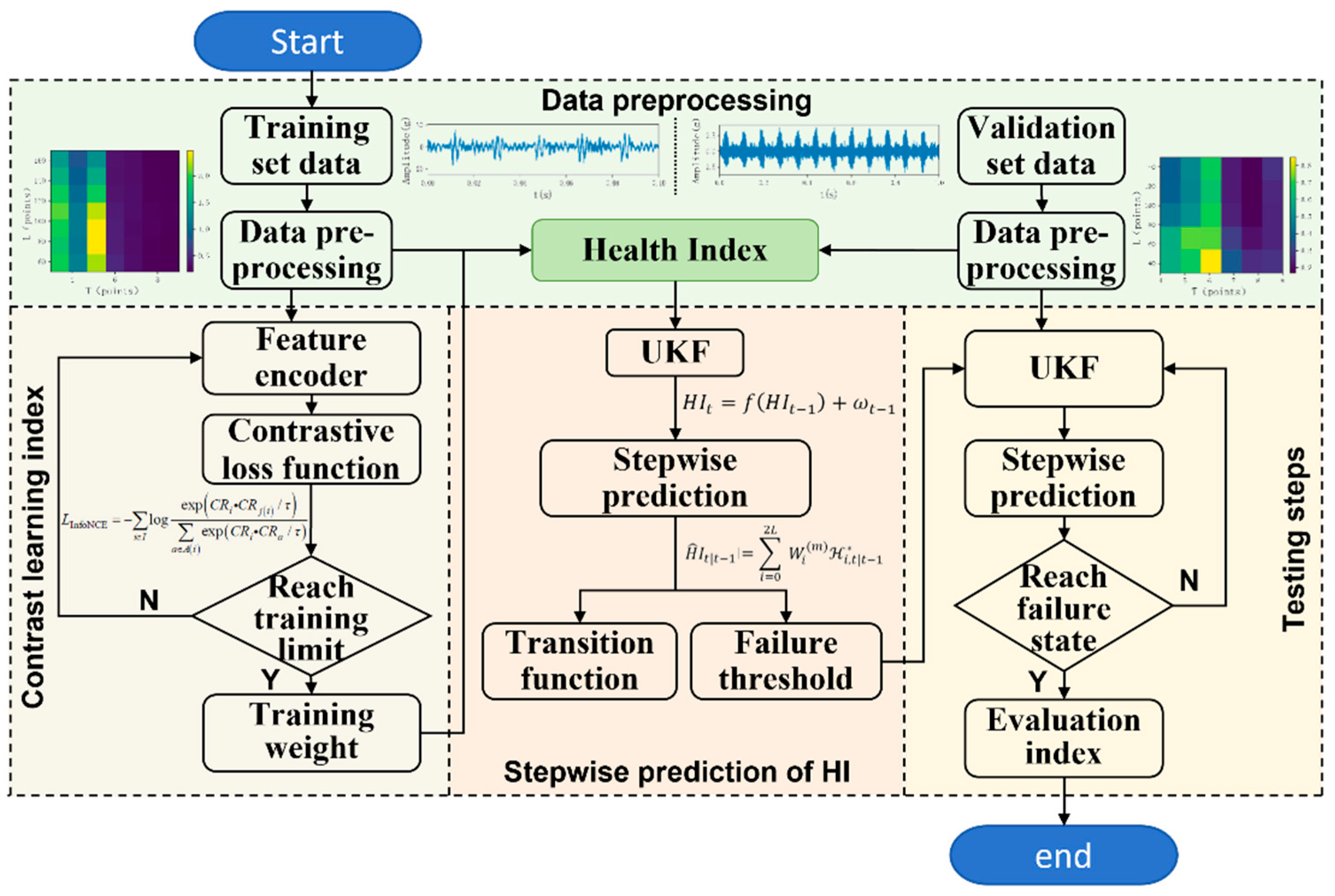
Figure 2.
Architecture of this HI-based RUL prediction model.
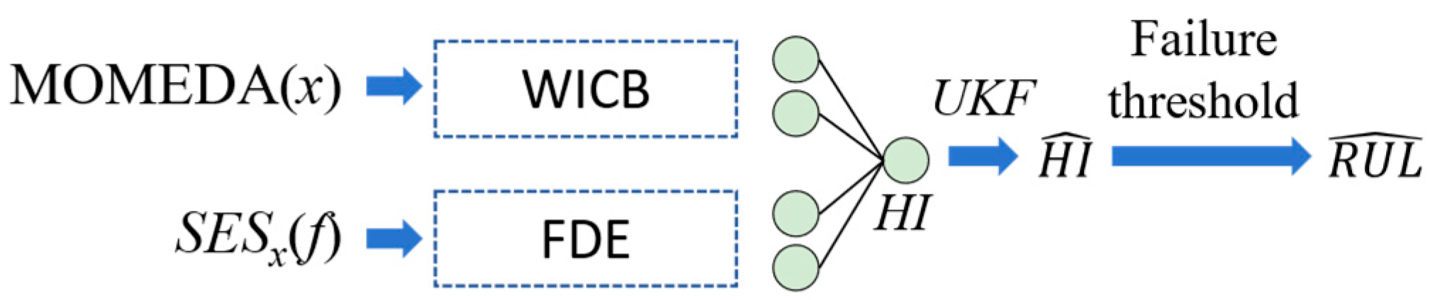
Figure 3.
Spiral bevel gear experiment platform.
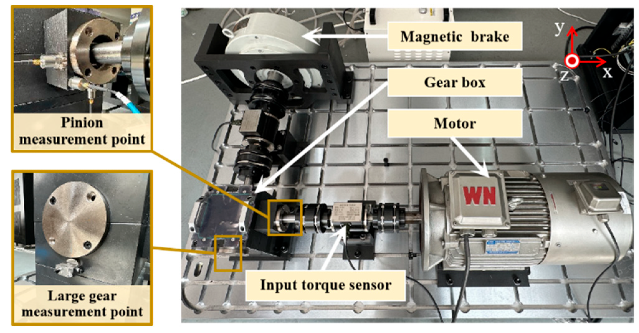
Figure 4.
HI based on contrastive learning in training and test set.
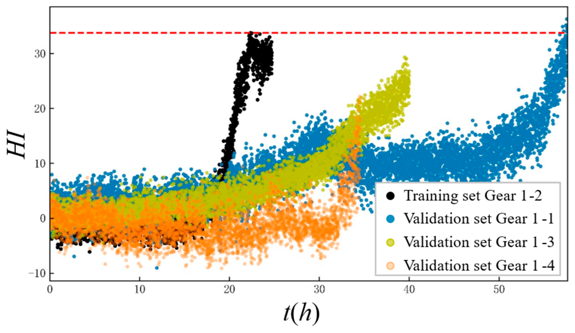
Figure 5.
Step-by-step prediction of HI based on UKF.
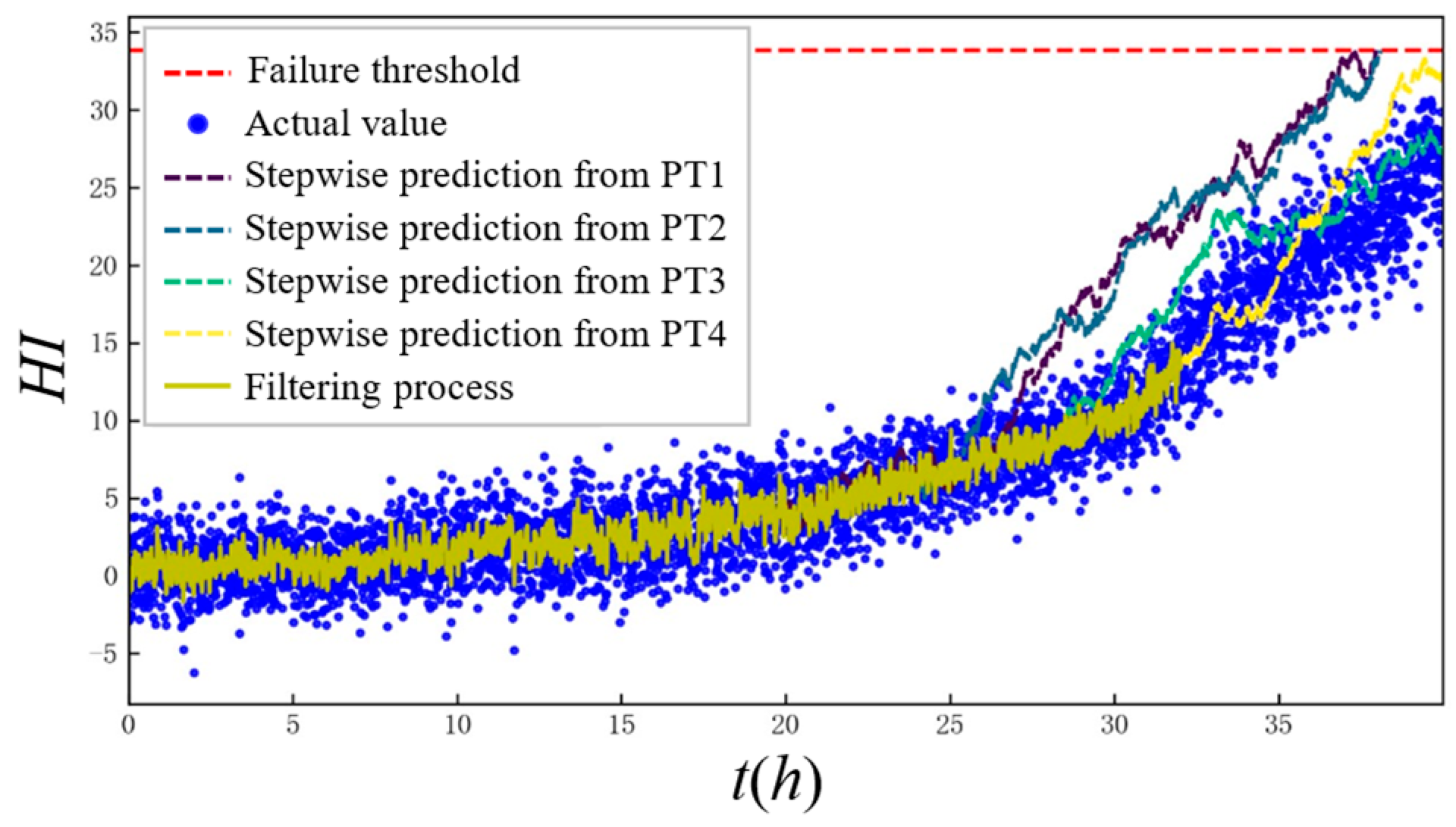
Figure 6.
HI comparison of (a) statistics, (b) PCMD, (c) DTC-VAE, (d) Proposed model.
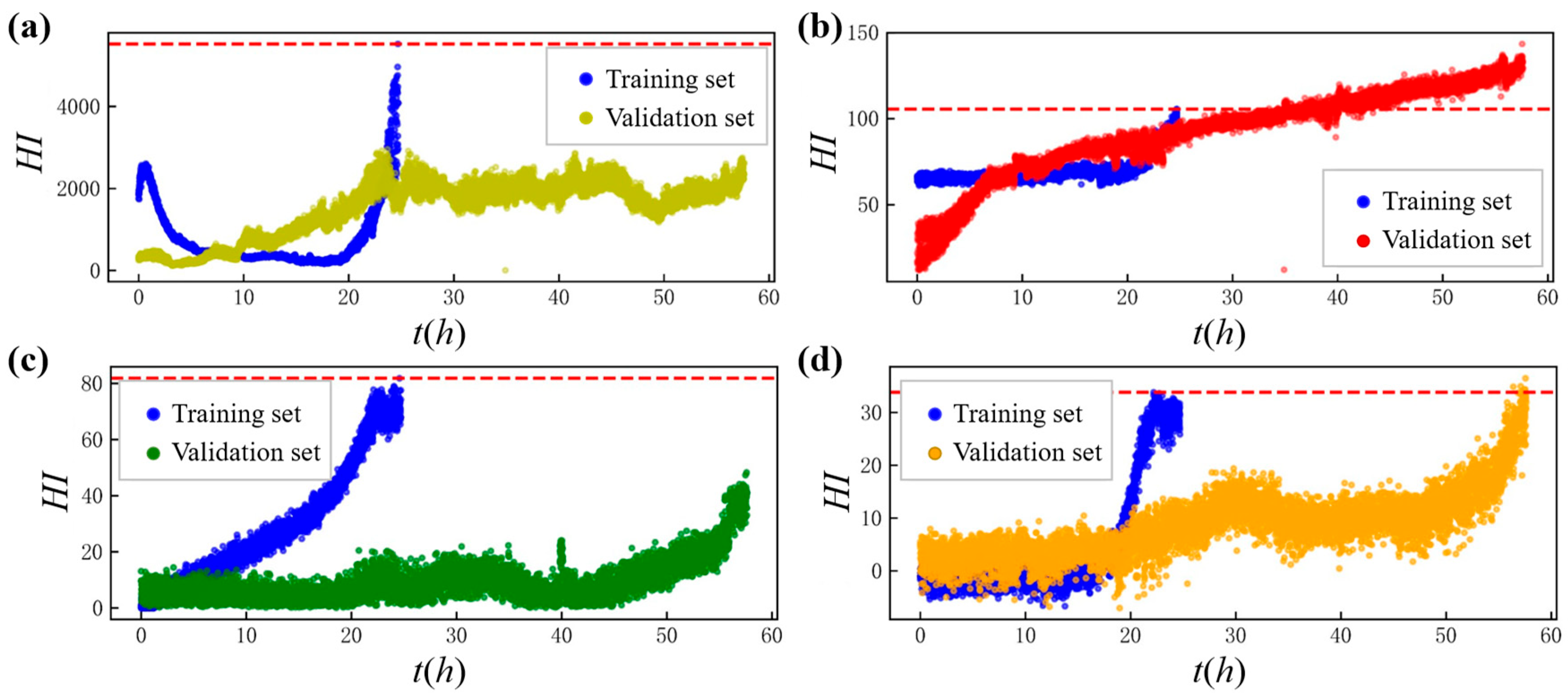
Figure 7.
RUL prediction results of different models by (a) statistics, (b) PCMD, (c) DTC-VAE, (d) Proposed model in XJTU-SY dataset and (e) statistics, (f) PCMD, (g) DTC-VAE, (h) Proposed model in spiral bevel gear dataset.
Figure 7.
RUL prediction results of different models by (a) statistics, (b) PCMD, (c) DTC-VAE, (d) Proposed model in XJTU-SY dataset and (e) statistics, (f) PCMD, (g) DTC-VAE, (h) Proposed model in spiral bevel gear dataset.
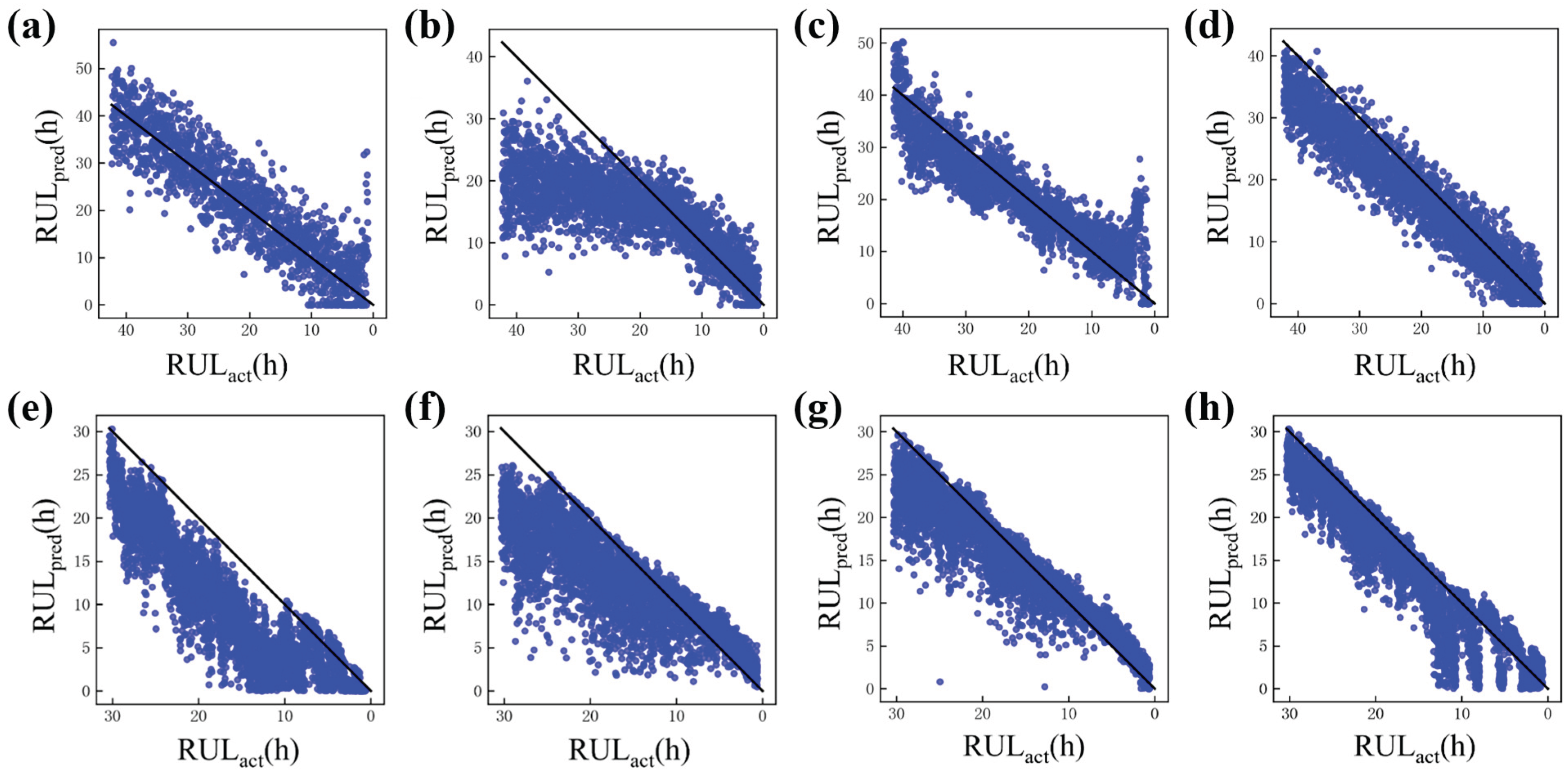

Table 1.
Hyper-parameters of RUL prediction model based on HI.
| Module | Object | hyperparameters | value |
| Data preprocessing | Spectrum envelope | Extraction index | [0:1024] |
| MOMEDA output | Extraction index | [0:1024] | |
| construction of HIs | Loss function | Temperature coefficient τ | 1 |
| Feature domain encoder | Size of the linear layer | (1024+358,1) | |
| Time domain encoder | Maximum pooling stride | 20 | |
| HI stepwise prediction | UKF | scale parameter α | 0.1 |
| Suboptimal parameters κ | 0 | ||
| Process noise covariance Q | 0.01 | ||
| Observation noise covariance R | 0.1 |
Table 2.
Parameters of spiral bevel gear dataset.
| Condition number | Input speed fr/rpm |
Input torque T/N·m |
Engage frequency fm/Hz |
Test gear number | Gear lifespan | failure mode |
| I | 1450 | 95 | 700.83 | Gear1-1 | 60 h 1 min | Condition 1 |
| Gear1-2 | 25 h 44 min | Condition 1 | ||||
| Gear1-3 | 41 h 39 min | Condition 1 | ||||
| Gear1-4 | 35 h 58 min | Condition 1 | ||||
| II | 1350 | 110 | 652.5 | Gear2-1 | 6 h 26 min | Condition 1 |
| Gear2-2 | 30 h 22 min | Condition 2 | ||||
| Gear2-3 | 20 h 58 min | Condition 1 | ||||
| Gear2-4 | 11 h 48 min | Condition 1 | ||||
| Gear2-5 | 13 h 25 min | Condition 1 | ||||
| III | 1250 | 125 | 604.17 | Gear3-1 | 18 h 16 min | Condition 1 |
| Gear3-2 | 11 h 6 min | Condition 1 | ||||
| Gear3-3 | 6 h 50 min | Condition 1 | ||||
| Gear3-4 | 16 h 57 min | Condition 1 | ||||
| Gear3-5 | 4 h 49 min | Condition 1 |
*Condition 1: Severe tooth surface adhesion, missing teeth; Condition 2: Tooth tip broken off, with the tooth surface flaked off.
Table 3.
HI metric comparison of different models.
| Model | XJTU-SY dataset | Spiral bevel gear dataset | ||||
| Monotonicity | relevance | robustness | Monotonicity | relevance | robustness | |
| statistics | 0.647 | 0.436 | 0.946 | 0.662 | 0.669 | 0.924 |
| PCMD | 0.485 | 0.714 | 0.981 | 0.494 | 0.858 | 0.968 |
| DTC-VAE | 0.547 | 0.764 | 0.894 | 0.612 | 0.794 | 0.722 |
| Proposed | 0.813 | 0.863 | 0.610 | 0.619 | 0.958 | 0.741 |
Disclaimer/Publisher’s Note: The statements, opinions and data contained in all publications are solely those of the individual author(s) and contributor(s) and not of MDPI and/or the editor(s). MDPI and/or the editor(s) disclaim responsibility for any injury to people or property resulting from any ideas, methods, instructions or products referred to in the content. |
© 2025 by the authors. Licensee MDPI, Basel, Switzerland. This article is an open access article distributed under the terms and conditions of the Creative Commons Attribution (CC BY) license (http://creativecommons.org/licenses/by/4.0/).
Copyright: This open access article is published under a Creative Commons CC BY 4.0 license, which permit the free download, distribution, and reuse, provided that the author and preprint are cited in any reuse.


