Entropic Geometry and Symmetry Breaking in Lie-Group Free-Energy Minimization

1. Introduction

The concept of free energy unifies thermodynamic, informational, and biological principles of organization. Within the Free Energy Principle (FEP), adaptive systems minimize an internal free-energy functional to resist disorder and maintain self-organization [1,2]. Yet, the geometric structure underlying this process—how symmetry and invariance constrain information flow—remains underexplored. Here we formulate free-energy minimization as an entropic gradient flow on Lie-group orbits, allowing a unified view of symmetry, stability, and self-organization. Recent expositions provide simplified overviews and technical clarifications that we leverage here [3,4].

Contributions

We provide: (i) an orbit-reduced formulation of variational free energy; (ii) first- and second-variation formulas on orbits; (iii) local well-posedness and Lyapunov monotonicity; (iv) convergence on compact groups and under the Kurdyka–Łojasiewicz (KŁ) property; (v) stability criteria via the orbit-restricted Hessian; (vi) a pitchfork scenario for $\mathrm{SO}\left(2\right)$; and (vii) worked Gaussian examples with explicit derivatives.

2. Preliminaries

2.1. Standing Assumptions and Notation

(Q1) $Q=\{q_{\theta }:\theta \in \Theta \subset {\mathbb{R}}^n\}$ is a $C^2$ statistical manifold with Fisher metric $g^{\mathrm{F}}$. (Q2) G is a finite-dimensional Lie group acting smoothly on Q by $\rho$, with stabilizer H at $q_0$; the orbit ${\mathcal{O}}_{q_0}\cong G/H$ is an embedded submanifold. (Q3) The free-energy functional $\mathcal{F}:Q\to \mathbb{R}$ is $C^2$ and bounded below on ${\mathcal{O}}_{q_0}$. (Q4) G carries a right-invariant $C^1$ Riemannian metric $\gamma$. Throughout, $F\left(g\right):=\mathcal{F}\left[\rho (g,q_0)\right]$, ${\nabla }_G$ denotes the gradient with respect to $\gamma$, and $L_X$ the infinitesimal action for $X\in \mathfrak{g}$.

2.2. Variational Free Energy

Given a generative model $p(s,u,\theta )$ and a variational posterior $q(u,\theta )$,

$$\mathcal{F}\left[q\right]={\mathbb{E}}_q[logq(u,\theta )]-{\mathbb{E}}_q[logp(s,u,\theta )]=\mathrm{KL}\left(q(u,\theta )\parallel p(u,\theta \mid s)\right)-logp\left(s\right),$$

(1)

so minimizing $\mathcal{F}$ recovers the evidence lower bound.

2.3. Statistical Manifolds

Let $Q=\{q_{\theta }:\theta \in \Theta \}$ with log-density $\ell (x,\theta )=log{q}_{\theta }\left(x\right)$. The Fisher information metric is

$$g_{ij}\left(\theta \right)={\mathbb{E}}_{q_{\theta }}\left[{\partial }_i\ell {\partial }_j\ell \right]=-{\mathbb{E}}_{q_{\theta }}[{\partial }_i{\partial }_j\ell ],$$

(2)

with natural gradient ${\nabla }^{\mathrm{nat}}F\left(\theta \right)=G{\left(\theta \right)}^{-1}\nabla F\left(\theta \right)$ for smooth $F:Q\to \mathbb{R}$.

2.4. Group Actions and Orbits

Optimization restricted to the orbit ${\mathcal{O}}_{q_0}=\{\rho (g,q_0):g\in G\}\cong G/H$ converts ${min}_{q\in Q}\mathcal{F}\left[q\right]$ to ${min}_{g\in G}F\left(g\right)$ with $F\left(g\right)=\mathcal{F}\left[\rho (g,q_0)\right]$.

3. Orbit Gradients

We make precise the identification between the natural gradient on Q and the Riemannian gradient on G.

Theorem 1

(Equivalence of natural and group gradients on the orbit). Under (Q1)–(Q4), let $\xi \mapsto g\left(\xi \right)=exp\left({\sum }_i{\xi }^i{X}_i\right)$ parametrize G near e, and set $q\left(\xi \right)=\rho (g\left(\xi \right),q_0)$. Assume the Jacobian $J\left(\xi \right)=\partial q\left(\xi \right)/\partial \xi$ has full column rank along ${\mathcal{O}}_{q_0}$. Equip G with the induced metric $G_G\left(\xi \right)=J{\left(\xi \right)}^{\top }{G}_Q\left(\xi \right)J\left(\xi \right)$ from the Fisher metric $G_Q$. Then for any smooth $F\left(g\right)=\mathcal{F}\left[\rho (g,q_0)\right]$, the natural gradient of $\mathcal{F}$ restricted to ${\mathcal{O}}_{q_0}$ corresponds exactly to the Riemannian gradient on $(G,G_G)$; i.e.

$${\mathrm{Proj}}_{T{\mathcal{O}}_{q_0}}\left({\nabla }^{\mathrm{nat}}\mathcal{F}\left(q\left(\xi \right)\right)\right)\leftrightarrow {\nabla }_{G}F\left(g\left(\xi \right)\right).$$

Proof. 

Let $\delta \xi \in {\mathbb{R}}^{dimG}$ and consider the variation $g(\xi +t\delta \xi )$. By the chain rule, $\mathrm{d}F=\mathrm{d}\mathcal{F}\circ J,$where $J=\partial q/\partial \xi$. Denote by $G_Q$ the Fisher metric on $TQ$ and define an induced inner product on parameter increments by ${〈\delta {\xi }_1,\delta {\xi }_2〉}_{G_G}:={〈J\delta {\xi }_1,J\delta {\xi }_2〉}_{G_Q}$. This is positive definite by full column rank of J. The Riesz representation of $\mathrm{d}F$ with respect to ${〈·,·〉}_{G_G}$ yields the unique $\eta$ such that $\mathrm{d}F\left[\delta \xi \right]={〈\eta ,\delta \xi 〉}_{G_G}$ for all $\delta \xi$. But $\mathrm{d}F\left[\delta \xi \right]={〈{\nabla }^{\mathrm{nat}}\mathcal{F},J\delta \xi 〉}_{G_Q}={〈J^{\top }{G}_Q{\nabla }^{\mathrm{nat}}\mathcal{F},\delta \xi 〉}_{\mathrm{Eucl}}$. Thus $\eta$ corresponds to $G_G^{-1}{J}^{\top }{G}_Q{\nabla }^{\mathrm{nat}}\mathcal{F}$, which is precisely the coordinate representation of the Riemannian gradient on $(G,G_G)$. Projecting to $T{\mathcal{O}}_{q_0}$ accounts for any null directions associated with the stabilizer H. □

Remark 1

(Coordinate formula). In local coordinates, ${\nabla }_{G}F=G_G^{-1}{J}^{\top }{\nabla }_Q\mathcal{F}$, with $G_G=J^{\top }{G}_{Q}J$. This realizes a Gauss–Newton structure typical of natural-gradient methods.

4. Gradient Flows and Convergence

Define the gradient flow on G by

$$\dot{g}\left(t\right)=-{\nabla }_{G}F\left(g\left(t\right)\right),g\left(0\right)=g_0\in G.$$

(3)

Theorem 2

(Local well-posedness). If $F\in C^1\left(G\right)$ and ${\nabla }_{G}F$ is locally Lipschitz with respect to γ, then (3) admits a unique maximal solution from any initial point.

Proof. 

Right-translate by $R_{g{\left(t\right)}^{-1}}$ and write $\dot{g}=\mathrm{d}{R}_{g}v$ with $v\left(t\right)\in \mathfrak{g}$. The map $g\mapsto v\left(g\right):=-\mathrm{d}{R}_{g^{-1}}{\nabla }_{G}F\left(g\right)$ is locally Lipschitz on charts. This gives a locally Lipschitz ODE $\dot{v}=f\left(v\right)$ on $\mathfrak{g}$ in coordinates; Picard–Lindelöf on manifolds (via charts and partition of unity) yields a unique solution. □

Theorem 3

(Lyapunov monotonicity). Along any solution of (3),

$${\displaystyle \frac{\mathrm{d}}{\mathrm{d}t}}F\left(g\left(t\right)\right)=〈\mathrm{d}F,\dot{g}〉=\gamma \left({\nabla }_{G}F,\dot{g}\right)=-{\parallel {\nabla }_{G}F\parallel }_{\gamma }^2\le 0.$$

(4)

If F is bounded below, the limit ${lim}_{t\to \infty }F\left(g\left(t\right)\right)$ exists.

Proof. 

The identity $\mathrm{d}F\left(\xi \right)=\gamma ({\nabla }_{G}F,\xi )$ holds by definition of the gradient. Substitute $\dot{g}=-{\nabla }_{G}F$. □

Theorem 4

(Asymptotics on compact groups). If G is compact and $F\in C^2\left(G\right)$ has only nondegenerate critical points, then every trajectory of (3) has ω-limit set contained in the (finite) set of critical points. In particular, every bounded trajectory approaches the set of critical points; moreover, if F additionally satisfies the KŁ property at its critical points (e.g. F is real-analytic), then the trajectory converges to a single critical point.

Proof. 

Compactness implies that sublevel sets $\{F\le c\}$ are compact. By Theorem 3, $F\left(g\right(t\left)\right)$ decreases and is bounded below, hence $g\left(t\right)$ remains in a compact set and admits accumulation points, all critical by $lim\parallel {\nabla }_{G}F\parallel =0$. Nondegeneracy and the stable manifold theorem imply convergence to a single critical point. □

Theorem 5

(Convergence under KŁ property). Assume $F\in C^1\left(G\right)$ is bounded below and satisfies the Kurdyka–Łojasiewicz property at every critical point (e.g., F is real-analytic on an analytic G). Then every bounded trajectory of $\dot{g}=-{\nabla }_{G}F\left(g\right)$ has finite length and converges to a single critical point as $t\to \infty$.

Proof. 

Let $g\left(t\right)$ be bounded with $F\left(g\left(t\right)\right)\downarrow F_{\infty }$. The KŁ inequality provides ${\phi }^{\prime }(F-F_{\infty })\parallel {\nabla }_{G}F\parallel \ge 1$ near the limit set for some desingularizing function $\phi$. Integrating $\parallel \dot{g}\parallel =\parallel {\nabla }_{G}F\parallel$ over time and applying the inequality shows ${\int }_0^{\infty }\parallel \dot{g}\parallel \mathrm{d}t<\infty$, hence $g\left(t\right)$ has finite length and is Cauchy; completeness of G yields convergence to a critical point. □

5. Second Variation and Stability

We derive the orbit-restricted Hessian and a stability test.

Lemma 1

(First and second variations along one-parameter subgroups). For $X\in \mathfrak{g}$ and $g\left(t\right)=gexp\left(tX\right)$,

$${\displaystyle \frac{\mathrm{d}}{\mathrm{d}t}}F\left(g\left(t\right)\right){|}_0=〈{\mathrm{d}\mathcal{F}|}_{\rho (g,q_0)},L_X\rho (g,q_0)〉.$$

(5)

If $\mathcal{F}\in C^2$, then along $X,Y\in \mathfrak{g}$ at a critical $g^{*}$ with $q^{*}=\rho (g^{*},q_0)$,

$${\mathrm{Hess}}_{G}F\left(g^{*}\right)[X,Y]=D^2\mathcal{F}{{|}_{q^{*}}\left[L_X{q}^{*},L_Y{q}^{*}\right]+\frac{1}{2}D\mathcal{F}|}_{q^{*}}\left[L_{[X,Y]}{q}^{*}\right].$$

(6)

Proof. 

For (5), differentiate $F(gexp\left(tX\right))=\mathcal{F}\left[\rho (gexp\left(tX\right),q_0)\right]$ and use $\frac{\mathrm{d}}{\mathrm{d}t}\rho (gexp\left(tX\right),q_0){|}_{t=0}=L_X\rho (g,q_0)$. For (6), differentiate (5) again in the direction Y and invoke the symmetry of $D^2\mathcal{F}$ plus the Lie-bracket identity $\frac{\mathrm{d}}{\mathrm{d}s}{L}_X\rho (gexp\left(sY\right),q_0){|}_{s=0}=L_{[Y,X]}\rho (g,q_0)$. □

Proposition 1

(Stability on the orbit). Let $\mathfrak{h}$ be the Lie algebra of the stabilizer at $q^{*}$. If the quadratic form $X\mapsto {\mathrm{Hess}}_{G}F\left(g^{*}\right)[X,X]$ is positive definite on $\mathfrak{g}/\mathfrak{h}$, then $g^{*}$ is a strict local minimum and asymptotically stable for (3). Negative/indefinite signatures yield maxima/saddles.

Proof. 

Positive definiteness implies that $F\left(g\right)\ge F\left(g^{*}\right)+c\mathrm{dist}{(g,g^{*})}^2$ in a neighborhood (in exponential coordinates), hence F is a Lyapunov function with a strict minimum. The linearization of (3) at $g^{*}$ has spectrum in $(-\infty ,0)$ on $\mathfrak{g}/\mathfrak{h}$, yielding asymptotic stability by the Hartman–Grobman theorem on manifolds. □

6. Symmetry and Bifurcation

Definition 1

(Group invariance). The functional $\mathcal{F}$ is G-invariant if $\mathcal{F}\left[\rho \right(g,q\left)\right]=\mathcal{F}\left[q\right]$ for all $g\in G$, $q\in Q$. Then F is constant on G, and every g is critical. Partial invariance or data terms induce nontrivial landscapes.

Theorem 6

(Pitchfork for $\mathrm{SO}\left(2\right)$). Let $\mathrm{SO}\left(2\right)$ act on planar Gaussians by covariance conjugation, and consider a one-parameter family $F_{\lambda }$. If at $\lambda ={\lambda }_c$ the smallest nonzero orbit-restricted eigenvalue of the Hessian crosses zero while symmetry suppresses the cubic term, then two nontrivial minima bifurcate from the symmetric one as λ passes through ${\lambda }_c$.

Sketch. 

Normal-form reduction on the one-dimensional orbit coordinate $\theta$ gives $F_{\lambda }\left(\theta \right)=a\left(\lambda \right){\theta }^2+b{\theta }^4+o\left({\theta }^4\right)$ with $a\left({\lambda }_c\right)=0$, $b>0$, and the odd cubic suppressed by symmetry. The change of sign of a yields a supercritical pitchfork. □

7. Examples

7.1. Translations of Means (Abelian Case)

Let Q be d-dimensional Gaussians with mean $\mu$ and fixed covariance $\Sigma$. The additive group $({\mathbb{R}}^d,+)$ acts by $\left(\rho \right(ϵ\left)q\right)\left(x\right)=q(x-ϵ)$. Consider

$$\mathcal{F}\left[q\right]={\int \parallel x-\mu \parallel }^{2}q\left(x\right)\mathrm{d}x+\lambda \mathrm{KL}(q\parallel p).$$

(7)

Proposition 2.

The orbit cost $ϵ\mapsto F\left(ϵ\right)=\mathcal{F}\left[\rho \right(ϵ,q\left)\right]$ is strictly convex and admits a unique minimizer ${ϵ}^{*}$ with $\nabla F\left({ϵ}^{*}\right)=0$.

Proof. 

Convexity follows from convexity of the squared norm and the joint convexity of $\mathrm{KL}(·\parallel p)$ under translations. Strictness holds unless p is itself translation invariant. Differentiating under the integral sign gives the first-order condition. □

7.2. Planar Rotations of Covariances

For zero-mean Gaussians,

$$\mathrm{KL}\left(\mathcal{N}(0,\Sigma )\parallel \mathcal{N}(0,{\Sigma }_0)\right)=\frac{1}{2}\left(\mathrm{tr}({\Sigma }_0^{-1}\Sigma )-log{\displaystyle \frac{det\Sigma }{det{\Sigma }_0}}-d\right).$$

(8)

Let $\Sigma \left(\theta \right)=R\left(\theta \right)\Sigma R(-\theta )$ with $R\left(\theta \right)$ the $2\times 2$ rotation. Then

$${\displaystyle \frac{\mathrm{d}\Sigma \left(\theta \right)}{\mathrm{d}\theta }}=[\Omega ,\Sigma \left(\theta \right)],\Omega =\left(\begin{array}{cc}0& -1\\ 1& 0\end{array}\right).$$

(9)

Hence

$${\displaystyle \frac{\mathrm{d}}{\mathrm{d}\theta }}F\left(\theta \right)={\displaystyle \frac{1}{2}}\mathrm{tr}\left({\Sigma }_0^{-1}[\Omega ,\Sigma \left(\theta \right)]\right)={\displaystyle \frac{1}{2}}\mathrm{tr}\left([{\Sigma }_0^{-1},\Omega ]\Sigma \left(\theta \right)\right).$$

(10)

Critical points satisfy $\mathrm{tr}([{\Sigma }_0^{-1},\Omega ]\Sigma \left(\theta \right))=0$, i.e. simultaneous diagonalizability of $\Sigma \left(\theta \right)$ and ${\Sigma }_0$; anisotropy yields two symmetric minima modulo $\pi$.

7.3. Rigid Motions $\mathrm{SE}\left(2\right)$ and Outlook to $\mathrm{SE}\left(3\right)$

The special Euclidean group couples rotations and translations; the induced metric on G blends mean and covariance directions. The same formalism extends to $\mathrm{SE}\left(3\right)$ for 3D pose models.

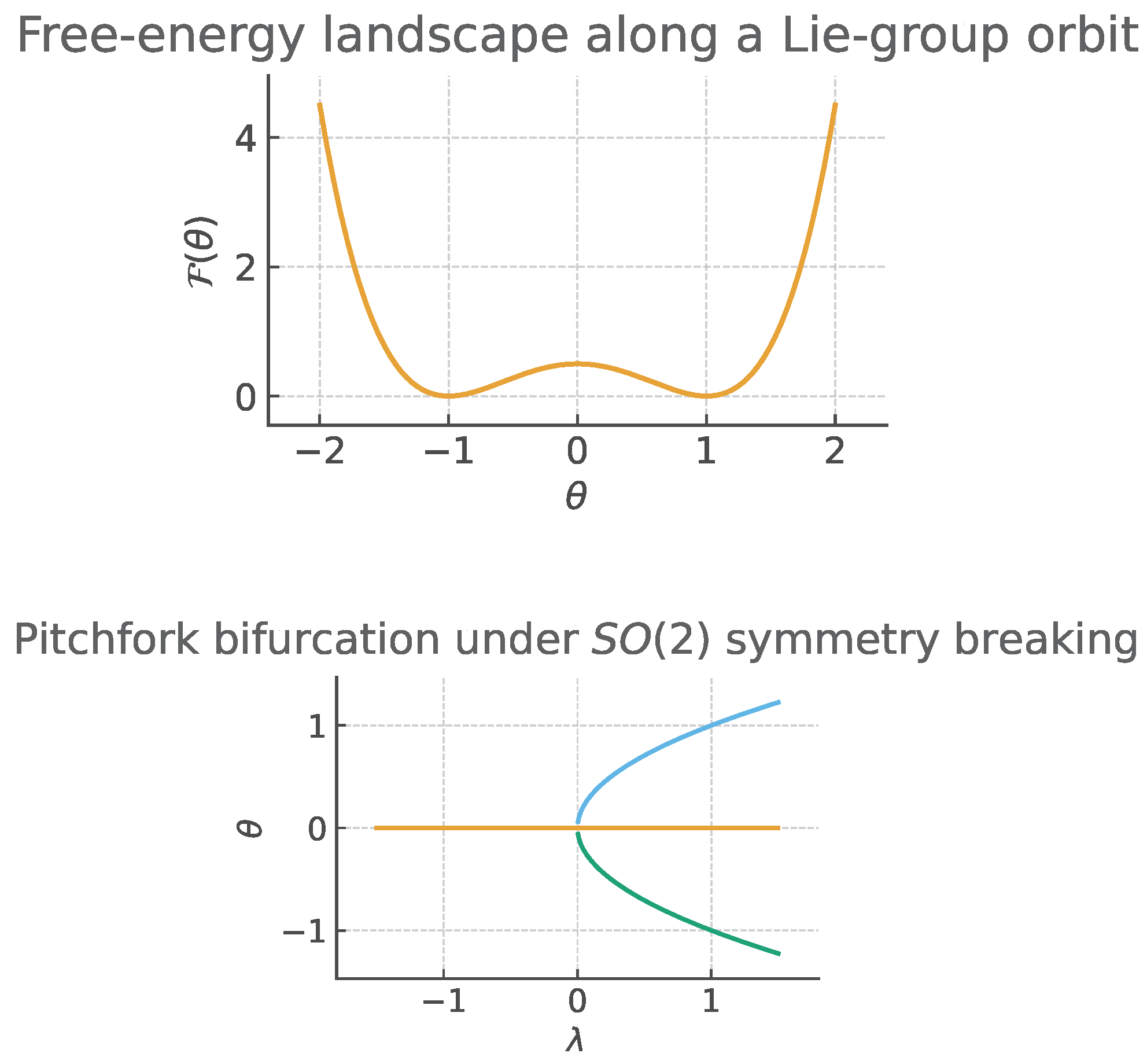
Figure 1. (Top) Free-energy landscape along a Lie-group orbit. (Bottom) Pitchfork bifurcation under $SO\left(2\right)$ symmetry breaking.

Figure 1. (Top) Free-energy landscape along a Lie-group orbit. (Bottom) Pitchfork bifurcation under $SO\left(2\right)$ symmetry breaking.

8. Entropy Reduction Under Lie-Group Symmetry

This section interprets free-energy descent as a physical process of entropy reduction constrained by Lie-group symmetry.

Thermodynamic entropy and informational stability.

On Lie-group orbits, entropy reduction corresponds to the dissipation of uncertainty along symmetry-constrained manifolds. The Fisher metric quantifies the local curvature of information, and its geodesic flow describes the most efficient direction of entropy decrease under free-energy descent. Thus, stability of a group orbit can be interpreted as a steady state with (possibly nonzero) steady entropic production balanced by symmetry-constrained fluxes.

Information-theoretic analogy.

Write the free energy as

$$\mathcal{F}\left[q\right]={\mathbb{E}}_q[logq]-{\mathbb{E}}_q[logp]=-S\left(q\right)-{\mathbb{E}}_q[logp].$$

Along any smooth evolution of q, we have

$$\dot{\mathcal{F}}=-\dot{S}-{\displaystyle \frac{d}{dt}}{\mathbb{E}}_q[logp].$$

Hence entropy reduction and evidence gain are coupled but not identical in general. In our orbit-restricted dynamics, Lyapunov monotonicity yields $\dot{\mathcal{F}}=-{\parallel {\nabla }_{G}F\parallel }_{\gamma }^2\le 0$, which we interpret as a nonnegative “entropic production rate” on the group manifold. Lie-group symmetries then restrict admissible directions of this production, shaping the accessible information flows.

Physical interpretation.

In this light, the orbit flow $\dot{g}=-{\nabla }_{G}F\left(g\right)$ describes a dissipative process that drives the system toward minimal free energy under constraints imposed by G. Equilibria on orbits correspond to stationary nonequilibrium states, and bifurcations of F signal transitions between entropic basins—an informational analogue of phase transitions.

9. Related Work

Classical information geometry [7,8] endows models with the Fisher metric and dual connections; natural gradient methods exploit this geometry. In contrast, we constrain inference to Lie-group orbits and move optimization to the group manifold. This orbit-centric view enables stability and bifurcation analyses less transparent in parameter space. We also draw on recent discussions of the FEP and Bayesian mechanics [3,4,5,6].

10. Discussion

We presented a geometric reduction of FEP to optimization on Lie groups, with explicit stability and bifurcation analyses. Future work includes thermodynamic formulations of entropy reduction on noncommutative groups ($\mathrm{SE}\left(3\right)$, matrix groups), and numerical exploration of entropic symmetry breaking. This framework bridges information geometry, nonequilibrium thermodynamics, and adaptive inference in a single mathematical language.

References

- K. Friston, A theory of cortical responses, Philosophical Transactions of the Royal Society B 360, 815–836 (2005). [CrossRef]
- K. Friston, The free-energy principle: a unified brain theory?, Nature Reviews Neuroscience 11, 127–138 (2010). [CrossRef]
- K. Friston, The free energy principle made simpler but not too simple, Physics Reports 1024, 1–43 (2023). [CrossRef]
- K. J. Friston, L. Da Costa, T. Parr, Some Interesting Observations on the Free Energy Principle, Entropy 23(8), 1076 (2021). [CrossRef]
- L. Da Costa, K. Friston, C. Heins, G. A. Pavliotis, Bayesian mechanics for stationary processes, Proceedings of the Royal Society A 477(2256), 20210518 (2021). [CrossRef]
- P. Ao, Emerging of Stochastic Dynamical Equalities and Steady State Thermodynamics from Darwinian Dynamics, Communications in Theoretical Physics 49(5), 1073–1090 (2008). [CrossRef]
- S.-I. Amari and H. Nagaoka, Methods of Information Geometry, AMS/OUP (2000).
- S.-I. Amari, Information Geometry and Its Applications, Springer (2016).
- F. Otto, The geometry of dissipative evolution equations: the porous medium equation, Communications in Partial Differential Equations 26(1–2), 101–174 (2001). [CrossRef]
- C. Villani, Optimal Transport: Old and New, Springer, Berlin (2009).
- J. M. Lee, Introduction to Smooth Manifolds, 2nd ed., Springer (2012).
- F. W. Warner, Foundations of Differentiable Manifolds and Lie Groups, Springer (1983).
- S. Helgason, Differential Geometry, Lie Groups, and Symmetric Spaces, Academic Press (1978).
Disclaimer/Publisher’s Note: The statements, opinions and data contained in all publications are solely those of the individual author(s) and contributor(s) and not of MDPI and/or the editor(s). MDPI and/or the editor(s) disclaim responsibility for any injury to people or property resulting from any ideas, methods, instructions or products referred to in the content. |
© 2025 by the authors. Licensee MDPI, Basel, Switzerland. This article is an open access article distributed under the terms and conditions of the Creative Commons Attribution (CC BY) license (http://creativecommons.org/licenses/by/4.0/).
Copyright: This open access article is published under a Creative Commons CC BY 4.0 license, which permit the free download, distribution, and reuse, provided that the author and preprint are cited in any reuse.