Submitted:
05 November 2025
Posted:
07 November 2025
You are already at the latest version
Abstract
Multi-arm caliper logging tools provide a high-precision technology for monitoring tubing and casing integrity. However, due to the wellbore structure of horizontal wells and the self-weight of the instrument, the multi-arm caliper logging data of horizontal wells typically exhibit obvious eccentricity, resulting in a high misjudgment probability in the quantitative evaluation of oil and casing pipe damage. In this manuscript, simulation experiments were conducted using the 5.5-inch casing under laboratory conditions. The experiments clarified the response characteristics of forty-arm caliper logging tools in centered and eccentric states within intact and damaged casing. An equivalent model combining the instrument and the horizontal pipe structure was established, and a new method for correcting instrument eccentricity based on the forty-arm caliper logging data in horizontal wells was developed through theoretical analysis. This model efficiently overcomes the limitation of existing eccentricity correction models in weakening damage detection under casing damage conditions. When compared with experimental data, the relative error between intact well section after eccentricity correction and centered measurement ranged from -4.93% to -0.72%, representing a reduction of 0.03% to 0.53% compared to the ellipse-fitting algorithm. The relative error between the response value of the damaged well section after eccentricity correction and centered measurement ranged from -5.02% to -0.45%, representing a reduction of 0.92% to 1.16% compared to ellipse-fitting algorithm. This effectively improves the correction coincidence rate for eccentricity influence of multi-arm caliper logging tools under various conditions in horizontal well. Applying this established method to the processing and interpretation of forty-arm caliper logging data in horizontal wells provides powerful technical support for the high-precision quantitative evaluation, damage location identification, and repair of horizontal well casing.
Keywords:
horizontal wells
; multi-arm caliper logging
; eccentricity influence
; instrument eccentricity position correction method
; casing damage evaluation
1. Introduction
Global demand for oil and natural gas continues to surge, making the exploitation and development of unconventional oil and gas reservoirs increasingly important for petroleum engineers [1,2]. Due to the poor physical properties of these unconventional reservoirs, horizontal wells and volume fracturing technology have emerged as effective development strategies [3,4]. However, several factors during development—such as hydraulic fracturing, corrosive fluid, and changes in crustal stress—can damage tubing and casing. Common types of damages include corrosion, misalignment, deformation, and perforation, and these damages significantly impair normal oil and gas production [4,5,6]. By 2021, Chinese oil fields reported over 30,000 wells with tubing and casing damage, with major fields all experiencing damage rates exceeding 20%. Globally, some oil fields face alarming casing failure rates of up to 50% [7,8]. Consequently, accurate detection and quantification of tubing and casing damage have become crucial for effective repair operations.
Monitoring tubing and casing damage presents major challenges, particularly in horizontal wells. The complexity of wellbore structure makes it challenging to transport logging instruments downhole and maintain proper centering, especially compared to vertical wells. Current casing damage monitoring technologies include multi-finger imaging tool, e.g., MIT [9,10,11,12] ultrasonic testing technology [13,14,15,16,17,18] and electromagnetic detection technology [19,20,21,22], e.g., MTT (Magnetic Thickness Tool) [13,22,23,24,25], MID-K/S (Magnetic Inspection Device-K/S) [26,27,28,29], TEM (Transient Electromagnetic Tool) [30,31,32], et al. Among these techniques, the MIT stands out as the most widely used method for wellbore integrity monitoring due to its effectiveness and cost efficiency. This mechanical device consists of equi-angular-spaced tungsten carbide-tipped arms that expand until they contact the inner casing surface. The logging system detects the damage by recording voltage signal variations caused by arm extension and retraction when contacting damaged inner surfaces. When measuring arm pass through the perforations, they extend; conversely, they retract when encountering scaling. To maximize coverage of the casing shaft section, MIT designs include varying numbers of arms (24, 40, 64, 80, and 120) suitable for different casing sizes. Despite this range, defects shorter than the circumferential distance between adjacent arms may remain undetected. Furthermore, the instrument’s relatively simple mechanical structure makes it susceptible to various influences, especially in horizontal wells. In horizontal well sections, the instrument’s gravity often causes eccentricity during measurement, even when stabilizers are installed [33,34,35]. This eccentricity phenomenon will finally cause the measured caliper values of each arm to differ from one another, and seriously impact the final interpretation and mislead casing damage identification. Therefore, it is necessary to perform eccentricity correction and then provide accurate information for the integrity evaluation of the casing in horizontal wells.
Current eccentricity correction methods for the MIT include opposite side compensation method [36], circle-fitting algorithm [35,37,38,39,40,41,42,43], center of mass method [40], chord approach [40,44], ellipse-fitting algorithm [41,43,44,45,46,47], and the confined best-fit circle method [44]. Among the methods, the opposite side compensation method asserts that the inner casing diameter is correctly measured under the instrument eccentricity condition. The changing symmetrical arm values are related; specifically, the increased value of extended arms and the decreased value of compressed arms correspond to the distance from the center position of the instrument. Therefore, the eccentricity is corrected by using symmetrical arm data. However, the method is only suitable for arms correction in the vertical direction, and is usually applicable for wells without any asymmetric damage and with a deviation angle of less than 45°. When the deviation angle exceeds 45° due to the excessive instrument eccentricity, the absolute sum of the opposite sides fails to reflect the true borehole diameter, creating a false impression of elliptical casing deformation [36]. The circle-fitting algorithm assumes a standard circular distribution of multi-arm caliper probes and uses circular function fitting to determine the center and radius in a two-dimensional coordinate system. Eccentricity-corrected arm values are calculated based on the center coordinates, geometrical coordinates, and corresponding azimuth angles [37,38,44]. While effective for undamaged sections, this method produces numerous erroneous judgments in damaged casing sections. Comparatively, the ellipse fitting method improves circle-fitting by using an ellipse equation to fit eccentric caliper data. It employs linear inversion to obtain ellipse model parameters and works for both elliptical and circular borehole shapes, in which circles are treated as special ellipse cases. This approach satisfies eccentricity correction requirements for most casing shapes, including elliptical casing breakouts. However, it fails in casing perforation cases or when severely eccentric tools have multiple arms falling into small keyseats [41,43,44,46]. The center of mass method treats arms as point mass objects with equal mass [37,38,40]. While simple for calculating estimated borehole centers, it cannot display the specific position and produces results with a systematic offset. The chord method is based on the rule of intersecting chords, assuming that when two chords intersect in a circle, the product of one chord’s segment lengths equals that of the other. In a circular borehole, opposite arm length products remain constant, allowing borehole center determination in gauge holes. However, this approach fails in non-circular boreholes where the intersecting chords rule no longer applies [40,44]. As a result, the center of mass method will always calculate a borehole center that is located halfway between the tool position and the real borehole center [40]. The confined best-fit circle method [45] obtains the confined best-fit circle center based on the restriction condition of confinement. It solves a least-squares problem with inequality constraints using the Lagrange multiplier method. This approach yields an accurate true virgin tool center when circular wellbore segments are preserved. Substantial borehole enlargement, such as washout, creates invalid hole flags for subsequent analysis [44]. While providing good fitting effects, this method applies only to open-hole logging without borehole shrinkage and fails to address casing damage scenarios [40,43,44].
Currently, no single method provides optimal decentralization corrections for an MIT across all situations. For undamaged tubing and casing, all methods are applicable, except for the center of mass method. The chord method shows best performance in a small key-seat scenario [40], while the circular algorithm provides satisfactory results [41]. For a large key-seat scenario, the ellipse-fitting method calculates tool centers accurately, though with a greater offset than the actual tool centers. Among the primary algorithms, ellipse-fitting and chord methods deliver the best tool for eccentricity corrections. However, methods that fit well diameter curves from instrument monitoring, including circle-fitting, ellipse-fitting, and chord approaches, often fail to detect localized casing damage. Comparison of the advantages and disadvantages of the existing eccentricity correction methods is listed in Table 1.
A new eccentricity correction method is needed for a MIT used in horizontal wells. Our proposed method aimed to perform corrections under various conditions, providing effective technical support for monitoring and evaluating tubing and casing damage in horizontal wells, precisely locating damage, and guiding repair operations.
The paper is organized as follows: Section 0 introduces the experiments and results, detailing comprehensive experimental steps and MIT logging outcomes. Section 1 presents our newly developed eccentricity correction method based on the described experiments. Section 3 discusses the correction effects of each method under damaged and intact casing conditions, comparing their error rates. Finally, we conclude by synthesizing the discussed analyses.
2. Experiments and Results
To simulate MIT response in horizontal wells, we conducted experiments using a 40-arm caliper logging tool at the Xinjiang Branch of China National Logging Group Co., Ltd. The experimental system consists of the ground information acquisition system, signal control and transmission system, 40-arm caliper logging tool, casing with different inner diameters, and damage designs. The 40-arm caliper logging tool (Figure 1) (WELL-SUN Company, Xi’an Shanxi, China) features an outside diameter of 2.875 in (73.03 mm) and a length of 61.97 in (1574.04 mm). The tool measurement range spans from 2.9 to 7.5 in (73.66–190.5 mm), with a radius measurement accuracy of ±0.03 in (±0.762 mm), and a resolution of 0.005 in (0.127 mm).
For simulating the horizontal well bore, we used 5.5 in (139.7 mm) diameter casing with a wall thickness of 7.72 mm. Each casing section measured 9.87 m in total length with damage (holes and cracks) distributed across 2.53 m (Figure 2 and Figure 3). We designed holes with varying diameters (49.5 mm and 29.8 mm) spaced at approximately 195 mm intervals. The cracks were designed in vertical and horizontal structures, measuring 1 and 3 cm in width, respectively. These diverse damage patterns allowed us to comprehensively evaluate the 40-arm caliper logging tool’s response under both centralization and eccentricity conditions.
The experiment steps are as follows:
First, the casing was horizontally fixed to simulate the horizontal wellbore. The 40-arm caliper logging tool was connected with the ground information acquisition equipment via a power cable and powered on to ensure a normal operation. Prior to formal measurement, we calibrated the tool using a standard graduated cylinder with five reference scales (3.125, 4, 5, 6, and 7 in). This calibration established a linear relationship between the instrument response and standard inner diameters to eliminate the systematic errors (Figure 4). It ensures that accurate measurements are obtained when the instrument is centered in the wellbore.
Secondly, we inserted the 40-arm caliper logging tool into the casing and positioned it at the toe of the casing. All measurement data were recorded during the uniform lifting process. We conducted measurements in both intact and damaged casings, and repeated both continuous logging and fixed-point measurement twice to ensure data stability and accuracy. For experiments with the damaged casing, we simulate eccentricity by omitting the centralizer from the multi-arm caliper logging tool string. After installation, we recorded continuous measurements during uniform upward tool movement, with repeated trials ensuring data reliability (Figure 5 and Figure 6). We then performed stationary point measurements under eccentric conditions at multiple depth positions under identical experimental parameters. Subsequently, we installed centralizers on the multi-arm caliper tool to achieve centralization, enabling comparative continuous and point measurements in both centralized and eccentric configurations for damaged casing evaluation. The continuous logging and discrete point measurements were followed by centralized measurements with centralizers during both constant-velocity tool movement and stationary acquisition phases (Figure 7). All experimental configurations incorporated repeated measurement principles to validate measurement repeatability and ensure experimental reliability. This comprehensive approach allowed us to establish the response characteristics of the 40-arm caliper logging tool under varying centralization conditions for both intact and damaged casing geometries.
The instrument response curves obtained from centering and eccentric measurements in both intact and damaged casings are shown in Figure 6, Figure 7, Figure 8 and Figure 9. Figure 6 and Figure 7 display measurement curves under central and eccentric conditions in an intact casing, respectively. In these figures, the first track indicates the hole and crack positions; the second track shows maximum, minimum, and average wellbore diameter values; and the third through sixth tracks present raw multi-caliper values from the first to second continuous measurements.
Figure 8 and Figure 9 illustrate the measurement curves of the instrument under central and eccentric conditions in a damaged casing. These curves demonstrate the extension of multi-caliper arms when the instrument passes through cracks and holes. At 51–52 m, the MIT curves of “broken eccentricity 1” and “broken eccentricity 2” on both sides present extensive extrusion signs, while the curve in the middle shows a pronounced increase, indicating casing damage at this position (Figure 8).
A detailed analysis of the results reveals several key observations. The first and repeated measurement curves acquired in the intact casing under central conditions appear as straight lines with nearly identical values, demonstrating excellent measurement repeatability (Figure 6). This consistency occurs as the centralized instrument maintains stable positioning within the undamaged casing. Despite the instrument being in an eccentric position, the “complete eccentricity 1” and “complete eccentricity 2” curves remain relatively straight without obvious deformation (Figure 7). This stability can be attributed to the intact casing, which enables the tool to maintain a stable eccentric state within the wellbore. During monitoring, the measurement signals exhibit minimal fluctuations, resulting in logging curves that appear as essentially straight lines.
The logging responses in the damaged casing with the instrument under central and eccentric conditions are shown in Figure 8 and Figure 9. Under central conditions, the MIT curves exhibit a relatively uniform overall distribution, with localized responses indicating cracks and holes. At crack locations, the logging curves display a serrated pattern, while at holes, the curves show partial subsidence forming single or double sharp tooth-like features. The most significant difference between central and eccentric conditions is the pronounced extrusion deformation under eccentric conditions, manifested as uneven curve distribution. The compressed sections of the curves are relatively densely packed and darker in color, while the stretched sections are relatively sparsely distributed and lighter in color. This phenomenon occurs because the instrument, under the combined influence of its own gravity and eccentric placement, causes the lower measuring arms to compress inward, resulting in underestimated caliper values, while the upper arms stretch outward, leading to overestimated caliper values. Comparing the logging data under central and eccentric conditions in Figure 8 and Figure 9, it is clear that eccentricity extensively impacts logging response. Meanwhile, significant differences in the maximum, minimum, and average inner diameter values are observed between the damaged and intact casing conditions depicted in these figures. When the casing is damaged, the instrument arms extend into holes and fractures, causing the caliper curves to vary in shape; when the casing is intact, the maximum, minimum, and average inner curves essentially overlap.
The cross-sectional views before and after eccentricity correction at a depth of 52 m under the condition of a damaged casing with a crack, are shown in Figure 10. When comparing the logging data before and after eccentricity correction, the 52 m raw data reveals an eccentric phenomenon (Figure 10). Instrument eccentricity can substantially cause misjudgment in the quantitative evaluation of oil and casing pipe damage. Therefore, establishing an accurate eccentricity correction method is crucial.
3. Method
For multi-arm caliper logging tools in the horizontal wells (Figure 11), measurement accuracy is heavily dependent on tool positioning. When the instrument is centrally positioned within the wellbore (Figure 11a), its accuracy reflects the true casing radius. However, when the instrument deviates from the center of the wellbore (Figure 11b), the measured data no longer reflect the true radius even in intact wellbores. Typically, measuring arms near the bottom of the wellbore are compressed, resulting in a decrease in caliper values, while arms near the top extend, causing increased measurements. Given the fixed length of each caliper arm, we can establish an equivalent model combining wellbore structure and instrument positioning. By placing this equivalent model into a two-dimensional coordinate system, we can determine the coordinates of the contact position between the multi-arms and the inner surface of the wellbore could be obtained, then the main task is to obtain the correct center position coordinates of the instrument.
The measured value of a forty-arm caliper logging instrument monitoring is Li (where i represents the arm serial number of the clockwise multi-arm caliper logging tool, with i=1,2,3,..., 40). The rotation azimuth of arm 1 is ROT1, with adjacent arm angles at 9-degree intervals. Using arm 1 as the x axis and arm 11 as the y axis, the center point of the instrument after eccentricity is taken as the origin of the rectangular coordinate system (0,0). The coordinates of the center wellbore cross-section points are represented by (x0, y0). In Figure 12, Figure 13, Figure 14 and Figure 15, the red circle denotes the inner wall of the wellbore, while the light-blue circle indicates the central position of the instrument before eccentricity and the grey-blue circle signifies its central position after eccentricity.
- (1)
- When there is no damage to the casing and an arm is located in the due north direction of the shaft section (Figure 12), the corresponding arm number is,
When no arm is precisely at the top position of the shaft, the closest instrument arm number relative to the top is,
A decision needs to be made on this matter,, ,
Then obtain the maximum offset distance of the symmetry arm,
The coordinates of the wellbore center are represented by (x0, y0)=(0,∆max)
The spatial coordinates of each arm before eccentricity are expressed as (xi, yi), the later eccentric coordinates are expressed as (xi’, yi’), [ ] is the integration operation; NO is the arm number of the top arm; ROT1 is the azimuth angle of arm 1 monitored by multi-arm well diameter logging instrument, max is the maximum offset distance, mm; Li is the measured well diameter value, mm.
Finally, the eccentricity correction is completed according to the relationship between the coordinate points (0, 0) of the center point of the instrument and the shaft section (0, Δmax) and the coordinates (xi’, yi’), and whether the set loss is judged according to the radius before the eccentricity and the radius after correction.
- (2)
- When the instrument undergoes both vertical and horizontal deviations (Figure 13), we determine the maximum deviation direction by analyzing the difference values between symmetrical arms. The maximum offset distance of the symmetry arm is,
The maximum offset azimuth calculation is as follows,
When ,
Then the central dot coordinates (x0, y0) are expressed as,
When ROTm≤180,
When ROTm>180,
When ,
Then the central dot coordinates (x0, y0) are expressed as,
When ROTm≤180,
When ROTm>180,
The spatial coordinates of each arm before eccentricity are expressed as (xi, yi), while post- eccentric coordinates are expressed as (xi’, yi’), ∆max is the maximum offset distance, mm; Li is the measured caliper value of the i-th arm, mm; Li+20 is the measured caliper value of the (i + 20)-th arm, mm; ROT1 is the azimuth angle of arm number 1 monitored by the multi-arm caliper logging tool, °; ROTm is the azimuth angle substituting the azimuth angle of the longest arm when calculating the offset azimuth angle, in degrees; Lm is the measured caliper value of the longest arm when calculating the offset azimuth angle, mm; ROTi is the azimuth angle of the i-th arm monitored by the multi-arm caliper logging tool, °; x0 is the abscissa value of the center point of the wellbore cross-section, and y0 is the ordinate value of the center point of the wellbore cross-section.
Finally, the eccentricity correction is completed based on the relationship between the coordinate points (0,0) of the center point of the eccentric instrument and the central dot coordinates (x0, y0) of the shaft section, and the eccentric coordinates (xi’, yi’). Casing loss is determined by comparing the radius before the eccentricity and the radius after correction.
- (3)
- When there are casing damages
For damaged casings with horizontal and vertical instrument deviation (Figure 14), we employ two complementary methods to determine the shaft section center coordinates, then average the results.
Using Method 1, we calculated the difference in casing symmetry arms and then sorted the resulting values.
If the sorted Δi decreases from the arm with the maximum difference and the decreasing difference is relatively uniform, there is no casing damage; when the inversion of one arm and the decreasing difference is abnormal, the serial position of the arm is damaged.
After determining the maximum offset direction of the instrument by sorting the subtraction value of the symmetry arm, the maximum offset distance of the symmetry arm is,
The maximum offset direction of the instrument is determined by the subtraction value of the symmetry arm, and the maximum offset distance of the symmetry arm is,
The calculation process of the maximum offset arm azimuth angle and the central dot coordinates is the same as Equations (4)–(9).
In the equation, Δmax is the maximum offset distance, mm; Sort is the difference sorting function; Δi is the offset of the i-number arm from the symmetry arm, mm; Li is the measured well diameter value of arm i, mm; Li+20 is the measured well diameter value of arm i+20, mm;
Method 2, it is known that the rotation azimuth angle of arm 1 is ROT1, and the angle between any adjacent arms is a constant 9 degrees. Using the difference of wall thickness to calculate the corresponding offset distance, and then the central dot coordinates of the shaft section (x0’, y0’) are obtained, the arm number of the top arm is,
Taking the arm i as the maximum offset distance, coordinates of the circular circle at the center of the wellbore section (x0’, y0’) are obtained,
The coordinate position of the center of the final shaft section can be expressed as(),
The spatial coordinates before eccentricity are expressed as (xi, yi), while the post-eccentric coordinates are expressed as (xi’, yi’). NO is the serial number of the top arm; ROT1 is the azimuth of arm 1 monitored by multi-arm caliper logging, Li is the observed value of arm i, mm; Li+20 is the measured value of arm i+20, mm; (x0’, y0’) is the center point coordinates of the wellbore section obtained by two perpendicular arms; (x0, y0) is the coordinates of the center obtained by two perpendicular arms; and (?x,?y) is the coordinates of the final wellbore section from Method 1 and Method 2.
Finally, the eccentricity correction is completed based on the relationship between the tool center point coordinate (0, 0), the shaft center coordinates (?x,?y), and the eccentric coordinate (xi’, yi’). Casing loss assessment is based on comparing the radius before eccentricity and the radius after correction.
By establishing the new eccentricity correction method of horizontal well diameter logging data, we obtained corrected multi-arm caliper logging response values that accurately reflect the structural characteristics and damage position of horizontal oil well casing. This approach effectively supports high-precision evaluation of multi-arm diameter monitoring data, ultimately enhancing oil well integrity assessment and repair planning.
4. Discussion
This study systematically validated the newly proposed eccentric correction method using experimental data and conducted a comprehensive comparative analysis with existing eccentric correction approaches. The results demonstrate that under intact casing conditions, all eccentric correction methods achieved satisfactory correction outcomes. However, in the presence of casing damage, our proposed method exhibited superior correction accuracy and stability compared to existing techniques. This superiority is thoroughly demonstrated by multiple sets of comparative experimental data (Figure 15, Figure 16, Figure 17 and Figure 18).
In Figure 15, Figure 16, Figure 17, Figure 18 and Figure 19, the gray solid line represents the standard casing outer diameter, the green solid line represents the standard casing inner diameter, and the red curve denotes the measured raw caliper data. Specifically, the opposite-side compensation method, circle-fitting algorithm, ellipse-fitting algorithm, chord method, center of mass method, and new eccentric correction method in the study are denoted by black, brown, teal, purple, light blue, and yellow, respectively. Under intact casing and instrument centering conditions (Figure 15), the measured caliper with the green standard inner diameter line requires no eccentricity correction. Figure 16 demonstrates the correction effects of each eccentric correction method under intact casing conditions with the instrument in an eccentric state. The raw caliper data only slightly deviate from the green standard inner diameter line, showing no obvious eccentric characteristics. This is because under single casing conditions, the cable exerts an upward force on the instrument, effectively counteracting the downward deviation caused by its gravity. Under these conditions, both the newly proposed eccentric correction method and the existing eccentric correction methods exhibit favorable correction effects.
Comprehensive result diagrams of various eccentricity correction methods under instrument eccentricity and centering conditions in a damaged casing are shown in Figure 17 and Figure 18. In Figure 17, each method displays an excellent correction performance under the condition of instrument centering in a damaged casing, the correction curves match the standard inner diameter. However, under eccentric conditions (Figure 18), a pronounced upward deviation of the original data curve from the standard inner diameter is evident. Specifically, the caliper measurements on the upper side exceed the standard inner diameter, whereas those on the lower side fall short. This phenomenon also indicates that there is a significant eccentricity in the instrument. This observation aligns precisely with the eccentric condition illustrated in Figure 10. Our systematic study of the fitting correction methods reveals major differences in their effectiveness. In areas with normal well conditions, all the tested correction techniques align with the standard inner diameter with high precision, resulting in excellent fitting outcomes. However, in damaged casing areas, the chord method, the opposite side compensation method, the circle-fitting algorithm, and even the relatively advanced ellipse-fitting algorithm all exhibit obvious limitations. These methods struggle to accurately identify damage features, which appear as sharp peaks in the fitting curves and ultimately lead to the omission of damaged areas. In contrast, the newly established eccentric correction method completely avoids these problems.
To present the differences among various correction methods, we conducted a comprehensive analysis for cases where the casing is damaged and the instrument is eccentric (Figures 19a)–f)).
Through a systematic comparative analysis, we found major performance differences among eccentricity correction methods. In normal well conditions, various methods achieve a good fit with the standard inner diameter, demonstrating an ideal correction effect. However, when applied to areas with damaged casings, traditional methods such as the chord method, the center of mass method, the opposite side compensation method, the circle-fitting algorithm, as well as the currently widely used ellipse-fitting algorithm, all reveal obvious limitations. The phenomenon is primarily attributed to the specialized measurement environment. In the damaged casing areas, when logging arms encounter holes, the measured data exhibit abnormal peaks, manifested as sharp protrusions in the fitting curves. Due to the algorithm limitations, traditional correction methods struggle to effectively identify and accurately process such abnormal data features. This often leads to the omission of this key damage information during the fitting process, thus affecting the accurate judgment of the actual condition of the casings. In sharp contrast, the newly proposed eccentric correction method demonstrates outstanding comprehensive performance advantages. Relying on its innovative algorithm design, this method not only maintains a high-precision fitting level in conventional areas but also, even when faced with complex scenarios of damaged casings, can accurately capture the damage features and achieve a high degree of consistency with the actual casing morphology, providing a more reliable technical support for detecting casing damage.
To further quantify performance disparities among correction methods and validate the advantages of the newly proposed method, this study conducted a systematic relative error analysis for each eccentric correction method. The results accurately reflect the differences in measurement accuracy and reliability among the methods, provide an important basis for evaluating their effectiveness in practical applications. The detailed data and analytical conclusions have been presented in Figure 20.
In-depth analysis of the relative error diagrams reveals that, under the conditions of both casing damage and instrument eccentricity, traditional correction methods exhibit notably wide relative error margins. Specifically, the opposite side compensation method shows a relative error range of -1.69% to 3.37%, the circle-fitting algorithm has a range of -1.72% to 3.60%, the chord approach yields a range of -1.69% to 3.63%, and the center of mass method demonstrates an even broader range, spanning from -1.92% to 3.71%. The conventional ellipse-fitting algorithm, while offering some improvement in correction efficacy, has managed to constrict its relative error range to -0.88% to 3.53%. In stark contrast, the newly proposed eccentric correction method significantly outperforms existing techniques. Its relative error range is confined to a much narrower interval of −0.61% to 0.66%, which represents a reduction of 0.27% to 2.87% compared to the ellipse-fitting algorithm. These findings unequivocally demonstrate that, in the challenging context of damaged casings and eccentric instrument positions, the new eccentric correction method attains the highest measurement precision and stability levels, thereby providing powerful technical support for the high-precision quantitative evaluation, damage location, and repair of the multi-arm caliper logging data of horizontal wells.
Based on the overall analysis, the eccentricity correction effects of the newly established eccentric correction method and the elliptical fitting correction method are relatively good. Therefore, an error analysis was conducted on the eccentric and centered data of the damaged and intact well sections for these two methods (Figure 21).
Experimental data comparisons indicate that the relative eccentric correction errors for intact casings are substantially lower than those for damaged casings. The new eccentric correction method demonstrates superior performance compared to the traditional ellipse-fitting algorithm. Specifically, for intact well sections, the relative error between the response values of eccentric and centered measurements, after applying the new correction method, ranges from -4.93% to -0.72%. This range reflects a 0.03–0.53% reduction in post-correction relative errors compared to the conventional ellipse-fitting algorithm. Conversely, for damaged well sections, the new method exhibits a relative error range of -5.02% to -0.45%, resulting in a 0.92–1.16% decrease in relative errors post-correction when compared with the traditional algorithm. These findings highlight that the proposed method effectively enhances the consistency of correcting the eccentric effects of multi-arm caliper logging tools for tubing and casing in horizontal wells across diverse damage scenarios, thereby contributing to more reliable well integrity assessments.
Our findings revealed that the newly proposed eccentric correction method, developed from the monitoring data of the forty-arm caliper logging tool, demonstrates remarkable technical advantages. This method excels in measurement precision and stability, and effectively addresses the issue of missing information in damaged well sections, a common drawback of traditional correction methods. As a result, it significantly expands the applicable scope. Whether under conventional or complex well conditions, this method is capable of accurately correcting the measurement deviations caused by eccentricity in multi-arm caliper logging data. It provides a solid and reliable technical guarantee for the efficient monitoring and evaluation of damage to the oil casing in horizontal wells, as well as for the precise location and scientific repair of such damage.
A relevant case analysis was conducted based on the newly proposed eccentric correction method (Figure 22). It illustrates the 3D correction diagrams of well sections before and after eccentricity correction. In the 3D imaging diagrams of typical well sections such as 3475–3500 m, 3640–3660 m, and 3835–3865 m, uncorrected data show major color differences in the 3D diagrams. Red regions represent casing damage, with caliper measurements exceeding the green-referenced standard inner diameter, while blue areas indicate borehole diameters smaller than the standard. This is because the eccentricity of the instrument and the casing damage lead to differences in the measured values of the borehole diameter. In contrast, corrected images show uniform color distribution dominated by the green reference, with substantially reduced red and blue regions, demonstrating regular morphological characteristics. This consistency intuitively confirms that the eccentricity correction effectively mitigates tool eccentricity effects. These results further validate the feasibility of the proposed method, which is of great significance for guiding casing damage detection and eccentric correction in field applications.
5. Conclusions
(1)This research provides valuable methodological advancements to horizontal well logging technology. Through a comprehensive comparative analysis of various eccentricity correction methods, a new eccentricity correction method was proposed and developed. Following data processing and correction, the results indicate that the newly proposed method exhibits the lowest relative error, showcasing its superior performance compared to existing techniques.
(2)Experimental data comparison reveals major improvement in measurement accuracy. For intact well sections, the relative error between the response values of eccentric and centered measurements after applying the new correction method spans from -4.93% to -0.72%. This range reflects a 0.03–0.53% reduction in post-correction relative errors compared to the conventional ellipse-fitting algorithm. Conversely, for damaged well sections, the new method exhibits a relative error range of -5.02% to -0.45%, resulting in a 0.92–1.16% decrease in relative errors post-correction when compared with the traditional algorithm. The proposed correction method addresses a critical limitation of existing approaches by accurately identifying and preserving damage features. Unlike traditional methods that often overlook localized casing damage, the proposed technique maintains high fidelity to actual casing conditions while simultaneously correcting for instrument eccentricity.
(3)The practical application of the eccentricity correction method significantly enhances the reliability of forty-arm caliper logging interpretation in horizontal wells. By extensively enhancing eccentricity correction accuracy, this method provides robust technical support for high-precision quantitative evaluation, precise damage localization, and efficient repair of horizontal well multi-arm wellbore logging data.This section is not mandatory but can be added to the manuscript if the discussion is unusually long or complex.
Author Contributions
Conceptualization, Xuemei Jian; methodology, Xuemei Jian; software, Meng Chen; validation, Xuemei Jian, Meng Chen, Xiangjun Liu, Guofeng Yang and Hongfa Ye; formal analysis, Xuemei Jian and Hongfa Ye; investigation, Xuemei Jian, Meng Chen, Xiangjun Liu, Guofeng Yang and Hongfa Ye; resources, Meng Chen, Xiangjun Liu and Yaning Zhao; data curation, Meng Chen, Xiangjun Liu and Yaning Zhao; writing—original draft preparation, Xuemei Jian and Meng Chen; writing—review and editing, Xuemei Jian, Meng Chen, Xiangjun Liu, Guofeng Yang, Hongfa Ye and Yaning Zhao; visualization, Xuemei Jian and Hongfa Ye; supervision, Meng Chen, Xiangjun Liu, Guofeng Yang and Yaning Zhao; project administration, Meng Chen; funding acquisition, Meng Chen and Yaning Zhao. All authors have read and agreed to the published version of the manuscript.
Funding
This project was supported by the Natural Science Foundation of Sichuan Province of China (No. 2024NSFSC1998) and the National Natural Science Foundation of China (No. 41804141). And this work was also supported by the Open Fund (PLN 201933) of State Key Laboratory of Oil and Gas Reservoir Geology and Exploitation (Southwest Petroleum University) and the China Postdoctoral Science Foundation (NO. 2018M643525).
Data Availability Statement
The data generated or analyzed during this study are available from the corresponding author upon reasonable request.
Acknowledgments
We would like to extend our heartfelt thanks to all those who provided support throughout the process of this work. Their contributions, whether in administrative assistance, technical help, or other forms, have been invaluable to the completion of this manuscript.
Conflicts of Interest
The authors declare no conflicts of interest.
Abbreviations
The following abbreviations are used in this manuscript:
| MIT | Multi-arm caliper logging tool |
| MTT | Magnetic Thickness Tool |
| MID-K/S | Magnetic Inspection Device-K/S |
| TEM | Transient Electromagnetic Tool |
References
- Jia, A.L.; Yan, H.J.; Tang, H.F.; Wang, Z.N.; Liu, Q.M. Key technologies and countermeasures for deep and ultra-deep gas reservoir development in China, Nat. Gas Ind. 2024, 44, 119–127. [Google Scholar]
- He, D.F.; Jia, C.Z.; Zhao, W.Z.; Xu, F.Y.; Luo, X.R.; Liu, W.H.; Tang, Y.; Gao, S.L.; Zheng, X.J.; Li, D.; Zheng, N. Research progress and key issues of ultra-deep oil and gas exploration in China. Pet. Explor. Dev. 2023, 50, 1333–1344. [Google Scholar] [CrossRef]
- Liao, Q.Z.; Wang, B.; Chen, X.; Tan, P. Reservoir stimulation for unconventional oil and gas resources: Recent advances and future perspectives, Adv. Geo-Energy Res. 2024, 13, 7–9. [Google Scholar] [CrossRef]
- Yin, H.; Zhao, X.W. ; LiQ; Gao, J.J.; Tang, Z.Q.; Dai, L.M. Effect of fracture-induced stress on casing integrity during fracturing in horizontal wells, Advances in Mechanical Engineering, Adv. Mech. Eng. 2022, 14, 1–9. [Google Scholar] [CrossRef]
- Yu, S.; Zhang, S.L.; Fu, J.H.; Shen, X.Y.; Yang, Z.L.; Guo, J.H.; Xiong, Y.L.; Li, B.; Peng, C. Analysis of casing stress during multistage fracturing of shale gas horizontal wells considering thermo-hydro-mechanical coupling, Energy Sci. Eng. 2023, 11, 2851–2865. [Google Scholar]
- Wu, T.J.; Li, M.; Liu, N.N.; Zhang, T.; Su, J.W. Research on mechanism of non-uniform in-situ stress induced casing damage based on finite element analysis, Appl. Sci. 2024, 14, 5987. [Google Scholar]
- Zhang, J.Q.; Wu, L.; Jia, D.L.; Wang, L.M.; Chang, J.H.; Li, X.N.; Cui, L.N.; Shi, B.B. “A machine learning method for the risk prediction of casing damage and its application in waterflooding,”. Sustainability 2022, 14, 14733. [Google Scholar] [CrossRef]
- Pan, Y.M. Study on the current situation and influencing factors of casing damage in S oilfield, Springer Series in Geomechanics and Geoengineering, 2020, pp. 2001-2006.
- Mohamed, H.; Osama, S.; Abdulhussein, F.; Lazăr, A. Pipe integrity analysis and evaluation using Multi Finger Imaging Tool (MIT)-field case studies, Pet. Coal 2021, 63, 455–466. [Google Scholar]
- Zeng, B.; Zhang, H.Z.; Zhou, X.J.; Gao, H. Microseismic characteristics of shale gas wells with casing deformation in Sichuan Basin, Paper presented at the 55th U. S. Rock Mechanics/Geomechanics Symposium, Virtual, Jun. 2021. [Google Scholar]
- Al-Haddad, S.M.; Shuber, H.H.; Alaryan, A.M.; Iqbal, P.; Nuriyev, O. Individual barriers corrosion monitoring using electromagnetic measurements, Paper presented at the SPE Thermal Well Integrity and Production Symposium, Banff, Alberta, Canada, Nov. 2022. [Google Scholar]
- Zhang, X.W.; Liu, J.D.; Cheng, W.; Jiang, W.D.; Jin, J.; Shen, L.H. New type of casing deformation rising in Weiyuan Changning shale gas play, Paper presented at the International Petroleum Technology Conference, Riyadh, Saudi Arabia, Feb. 2022. [Google Scholar]
- Ajgou, N.; Graba, B.; Sayah, L.; Ismail, M.; Yakupov, A.; Saada, M.; Rourke, M.; Abdelmoula, M. Effective solutions to well integrity management using multi finger caliper and electromagnetic tool, Paper presented at the SPE Gas & Oil Technology Showcase and Conference, Dubai, UAE, Oct. 2019. [Google Scholar]
- Chen, H.H.; Sun, Z.F.; Liu, X.E.; Qiu, A. Multifunctional ultrasound imaging logging tool design for casing wells of offshore oilfield in China, Paper presented at the The Twenty-fourth International Ocean and Polar Engineering Conference, Busan, Korea, Jun. 2014. [Google Scholar]
- Benayad, S.; Baouche, R.; Chaouchi, R.; Mitra, S.; Sen, S.; Benmamar, S. In-situ stress state and geomechanical modeling of the paleozoic clastic reservoirs in Hassi Terfa field, Algeria, Paper presented at the International Geomechanics Conference, Kuala Lumpur, Malaysia, Nov. 2024. [Google Scholar]
- Lu, J.Q.; JHan, Y.; Wu, J.P.; Che, X.H. ; QiaoWX; Wang, J. L.; Chen, X. Physical simulation of ultrasonic imaging logging response, Sensors 2022, 22, 9422. [Google Scholar]
- Hamadani, A.; Sawafi, S.A.l.; Taher, A. Acquiring high-resolution images while drilling in a fast logging environment utilizing a new ultrasonic sensor, Paper presented at the SPE Conference at Oman Petroleum & Energy Show, Muscat, Oman, Apr. 2024. [Google Scholar]
- Wang, J.; Liu, F.; Xu, H.H. Oil and gas casing 3D visualization technology based on multi-frequency ultrasonic scanning, Pet. Sci. Technol. 2023, 41, 1328–1348. [Google Scholar]
- Teplukhin, V.K. The development of theoretical foundations for electromagnetic flaw detection of oil and gas wells, Russ. J. Nondestr, Test 2004, 40, 834–843. [Google Scholar] [CrossRef]
- Bo, D.; Mengmeng, P.; Bowen, R.; Ling, Y. A signal reconstruction method for memory-type transient electromagnetic detection systems in horizontal wells, in 2021 3rd International Conference on Intelligent Control, Measurement and Signal Processing and Intelligent Oil Field (ICMSP), IEEE, 2021; pp. 63-67.
- Xie, Y.; Fan, L.H.; Yang, L.; Zhao, Y.; Hao, X.N.; Dang, B. Depth-time dimension signal reconstruction of transient electromagnetic logging using compressed sensing, in 2022 4th International Conference on Intelligent Control, Measurement and Signal Processing (ICMSP), IEEE, 2022.
- Ma, X.H. “Integrity of gas reservoir storage facilities during the operation phase,” handbook of underground gas storages and technology in China, (2021) 1-26.
- Zou, H.L.; Wang, X.G.; Kang, J.L.; Deng, M.M.; Wang, Q.H.; Zhu, H.S.; Gao, C.W. Integrated workover and re-completion techniques to successfully restore productivity for sour gas field,” Turkmenistan, Paper presented at the SPE Production and Operations Symposium, Oklahoma City, Oklahoma, USA, Mar. 2011. [Google Scholar]
- Elendu, C.; Nwamara, N.; Alinnor, C.; Enekhai, H.; Ojukwu, I.; Ayoo, J.; Abolarin, O. The diagnostics and recompletion strategy of a well with sustained casing pressure, Paper presented at the SPE Nigeria Annual International Conference and Exhibition, Lagos, Nigeria, Aug. 2022. [Google Scholar]
- Aliko, E.; Casciaro, D.; Conte, A.; Busollo, C.; Baronio, E.; Abdo, E.A. optimizing well integrity with accurate forecasting of casing and tubing resistance reduction trends through innovative numerical modeling techniques. SPE J. 2025, 30, 127–143. [Google Scholar] [CrossRef]
- Y.G. Zhao, L.Z. Y.G. Zhao, L.Z. Song, Casing defect detection logging and its application. Nat.Gas Ind. 2008, 28, 52–54. [Google Scholar]
- Li, Q.W.; Yang, Q.A.; Dong, X.H.; Li, M.X.; Xi, Y.T. Development of double layer metal thermal spray: Novel external corrosion mitigation method for gas well tubing, Paper presented at the SPE International Conference & Workshop on Oilfield Corrosion, Aberdeen, UK, May 2012.
- Zhong, X.F.; Wu, Y.X.; Qiang, L.; Yao, X.W. Multi-pipe string electromagnetic detection tool and its applications, 2007 8th International Conference on Electronic Measurement and Instruments, IEEE, 2007.
- Golovatskaya, G.; Potapov, A.; Xie, M.J.; Shumilov, A. The technology of magnetic-pulse flaw detection-thickness measurement of multistring wells by the transient method. Paper presented at the SPWLA 65th Annual Logging Symposium, Rio de Janeiro, Brazil, May 2024.
- Zhu, Y.L.; Chen, W.Y.; Song, W.T.; Han, S.X. New fast imaging techniques for electrical source transient electromagnetic data: Approaches and application, Computers & Geosciences, 2025; pp. 105770.
- Dutta, S.; Olaiya, J. Analysis and interpretation of multi-barrier transient electromagnetic measurements. Paper presented at the SPWLA 61st Annual Logging Symposium, Virtual Online Webinar, Jun. 2020. [Google Scholar]
- Xue, G.Q.; Li, H.; He, Y.M.; Xue, J.J.; Wu, X. Development of the inversion method for transient electromagnetic data, IEEE Access 2020,8, 146172-146181.
- Dang, B.; Yang, L.; Liu, C.Z.; Zheng, Y.H.; Li, H.; Dang, R.R.; Sun, B.Q. A uniform linear multi-coil array-based borehole transient electromagnetic system for non-destructive evaluations of downhole casings. Sensors 2018, 18, 2707. [Google Scholar] [CrossRef] [PubMed]
- Arshad, W.; Khan, K. Understanding the key factors affecting well integrity in horizontal well multistage hydraulic fracturing, Paper presented at the Middle East Oil, Gas and Geosciences Show, Manama, Bahrain, Feb. 2023. [Google Scholar]
- Li, H.Q.; Wang, R.H. Research on a measurement method for downhole drill string eccentricity based on a multi-sensor layout. Sensors 2021, 21, 1258. [Google Scholar] [CrossRef] [PubMed]
- Ning, W.D.; Hou, Y.W.; Liu, R.F.; Ma, L.J.; Liu, J.K. Multiarm well bore log correction evaluation technique, 2015 International Conference on Oil and Gas Field Exploration and Development, Xi’an, Shaanxi, Sep. 2015.
- Bäßler, H. Dezentrierungskorrektur von BHTV-Daten angewandt auf die Tiefbohrung VGS, Rußland: Hochauflösende Kaliberauswertung am Beispiel der KTB, 1995.
- Barton, C.A. Development of in situ stress measurement techniques for deep drillholes, Stanford University, 1988.
- P. Lysne, Determination of borehole shape by inversion of televiever data: The log analyst, The Log Analyst, 1986, 27, 64–71.
- Wagner, D.; Müller, B.; Tingay, M. Correcting for tool decentralization of oriented six-arm caliper logs for determination of contemporary tectonic stress orientation. Petrophysics 2004, 45, 530–539. [Google Scholar]
- Han, Z.Q.; Wang, C.Y.; Wang, Y.T.; Wang, C. Borehole cross-sectional shape analysis under in situ stress, Int. J. Geomech 2020, 20, 1–6. [Google Scholar]
- Assanelli, A.P.; Turconi, G.L. Effect of measurement procedures on estimating geometrical parameters of pipes, Paper presented at the Offshore Technology Conference, Houston, Texas, Apr. 2001. [Google Scholar]
- Sawaryn, S.J.; Pattillo, P.D.; Brown, C.; Schoepf, V. Assessing casing wear in the absence of a baseline caliper log. SPE Drill Completion 2015, 30, 152–163. [Google Scholar] [CrossRef]
- Yang, Z.T.; Fang, X.D.; Huang, L. A robust approach for determining borehole shape from six-arm caliper logs. Geophysics 2018, 83, 203–215. [Google Scholar] [CrossRef]
- Chandrasekhar, S.V.; Anjos, J.L.; Frazão, L.E.; Bonelli, R.C.; Percy, J.G.; Dos Santos, C.M.; Gasparetto, D.; Lima, L.B.; Pilisi, N. Casing wear estimation without a baseline log-a distorted ellipse methodology, Proceedings of the Annual Offshore Technology Conference, Texas, USA, 19. 20 May.
- Sawaryn, S.J.; Jamieson, A.L.; McGregor, A.E. Explicit calculation of expansion factors for collision avoidance between two co-planar survey error ellipses, Paper presented at the SPE Annual Technical Conference and Exhibition, San Antonio, Texas, USA, Oct. 2012. [Google Scholar]
- Markley, M.E.; Last, N.; Mendoza, S.; Mujica, S. Case studies of casing deformation due to active stresses in the andes cordillera, colombia, Paper presented at the IADC/SPE Drilling Conference, Dallas, Texas, Feb. 2002. [Google Scholar]
Figure 1.
The forty-arm caliper logging tool used in this study.
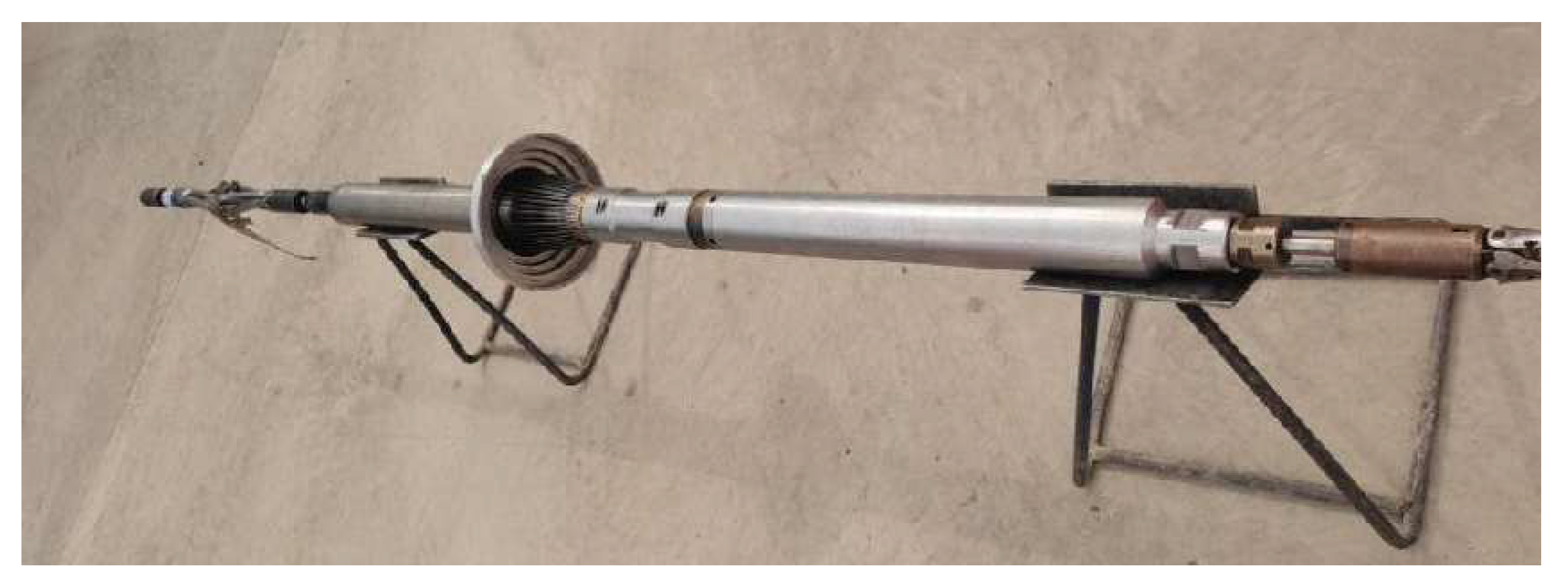
Figure 2.
Simulation experiment platform used in this study.
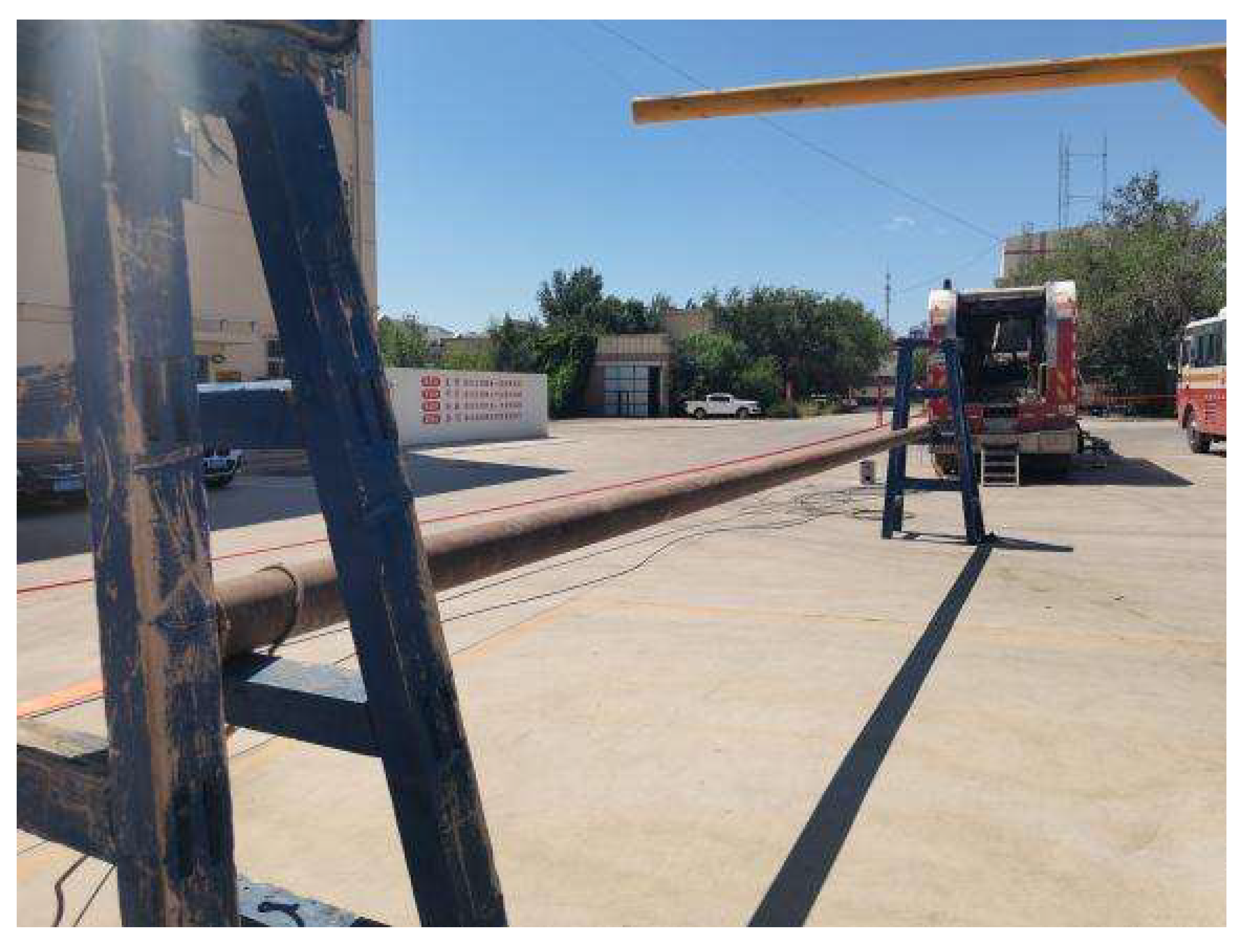
Figure 3.
Images of artificially-made holes and cracks used in this study.
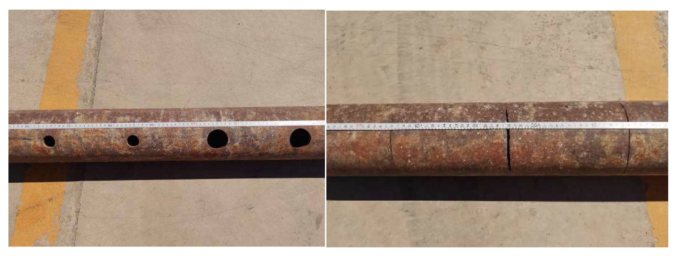
Figure 4.
Calibration of the multi-caliper logging tool used in this study.
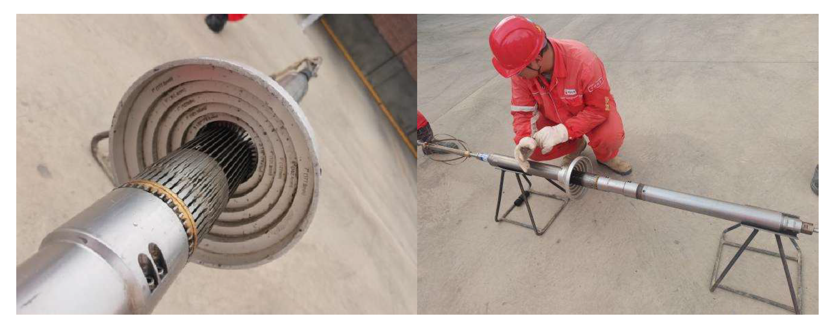
Figure 5.
Eccentric passage of the caliper logging tool through the casing and holes used in this study.
Figure 5.
Eccentric passage of the caliper logging tool through the casing and holes used in this study.
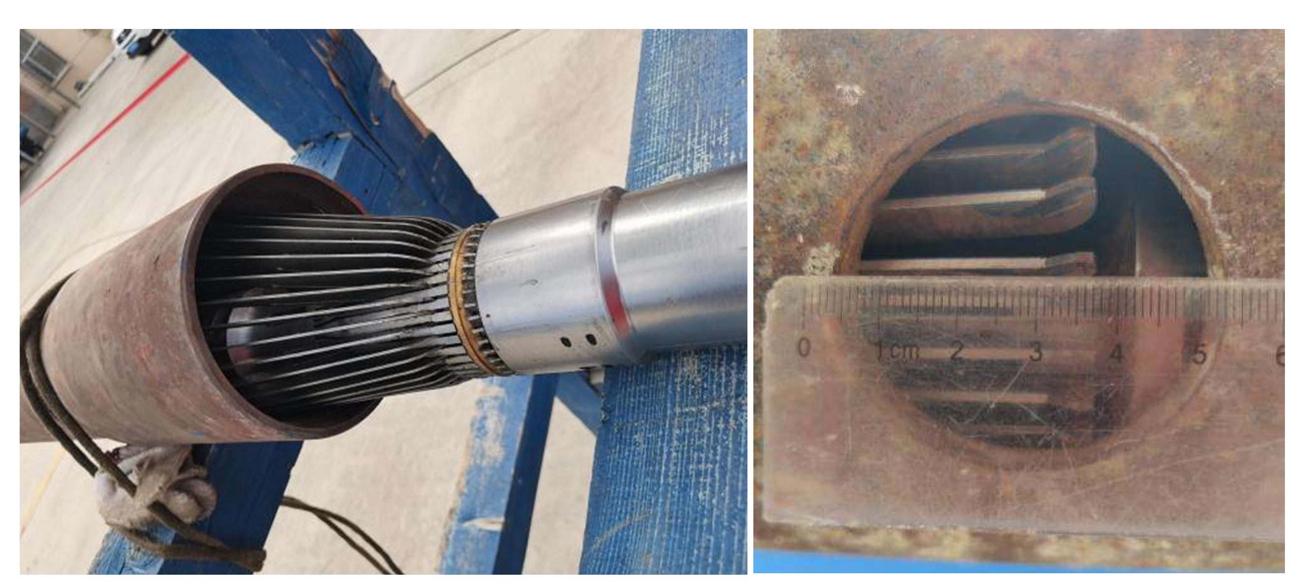
Figure 6.
The initial and repeated measurement curves in the intact casing when the instrument is under a centralized condition.
Figure 6.
The initial and repeated measurement curves in the intact casing when the instrument is under a centralized condition.
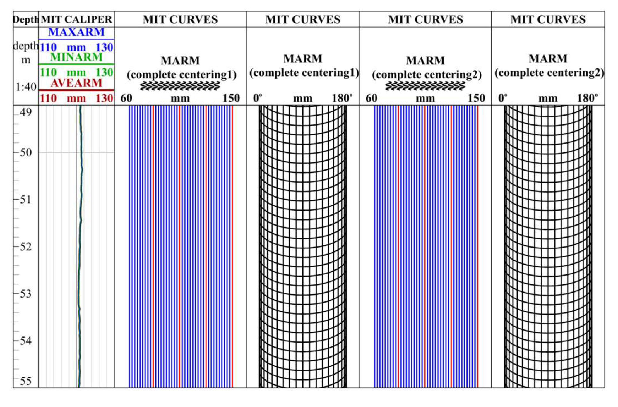
Figure 7.
The initial and repeated measurement curves in the intact casing when the instrument is under an eccentric condition.
Figure 7.
The initial and repeated measurement curves in the intact casing when the instrument is under an eccentric condition.
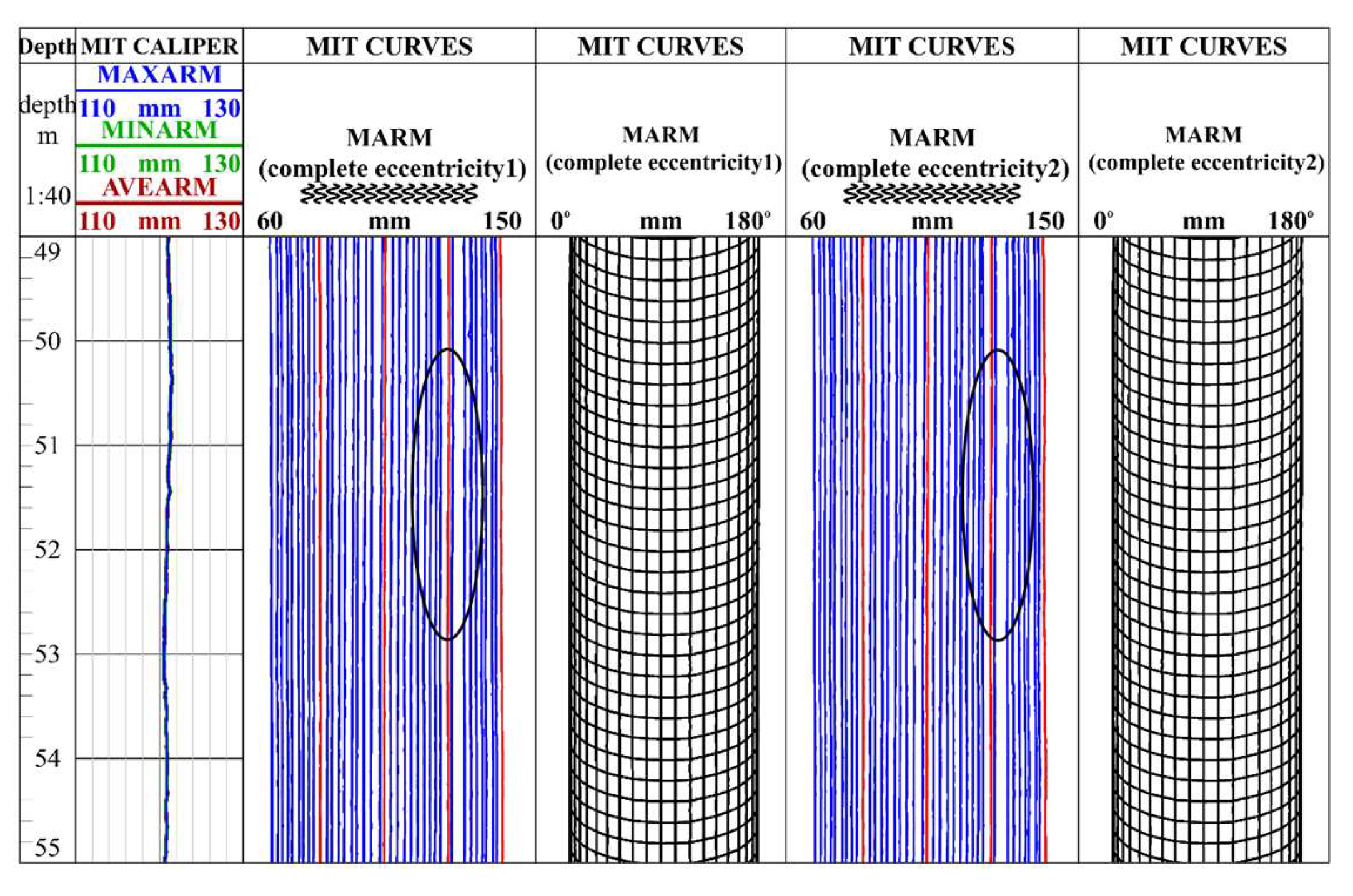
Figure 8.
The initial and repeated measurement curves in the damaged casing with different holes and cracks when the instrument is under a centralized condition.
Figure 8.
The initial and repeated measurement curves in the damaged casing with different holes and cracks when the instrument is under a centralized condition.
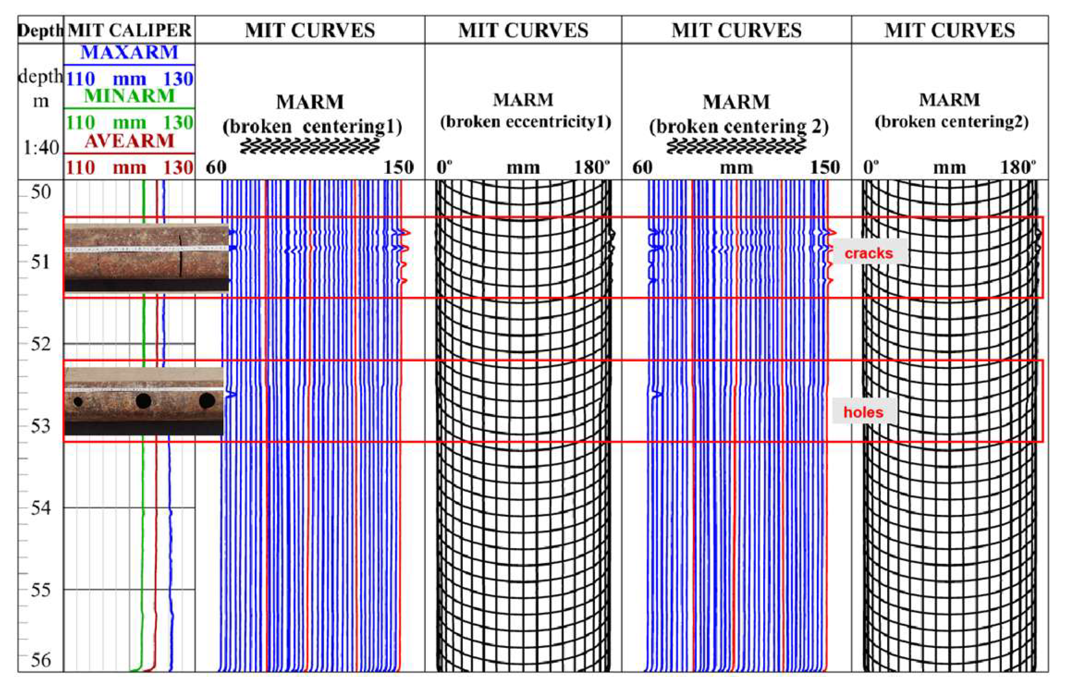
Figure 9.
The initial and repeated measurement curves in the damaged casing with different holes and cracks when the 40-arm caliper logging tool is under an eccentric condition.
Figure 9.
The initial and repeated measurement curves in the damaged casing with different holes and cracks when the 40-arm caliper logging tool is under an eccentric condition.
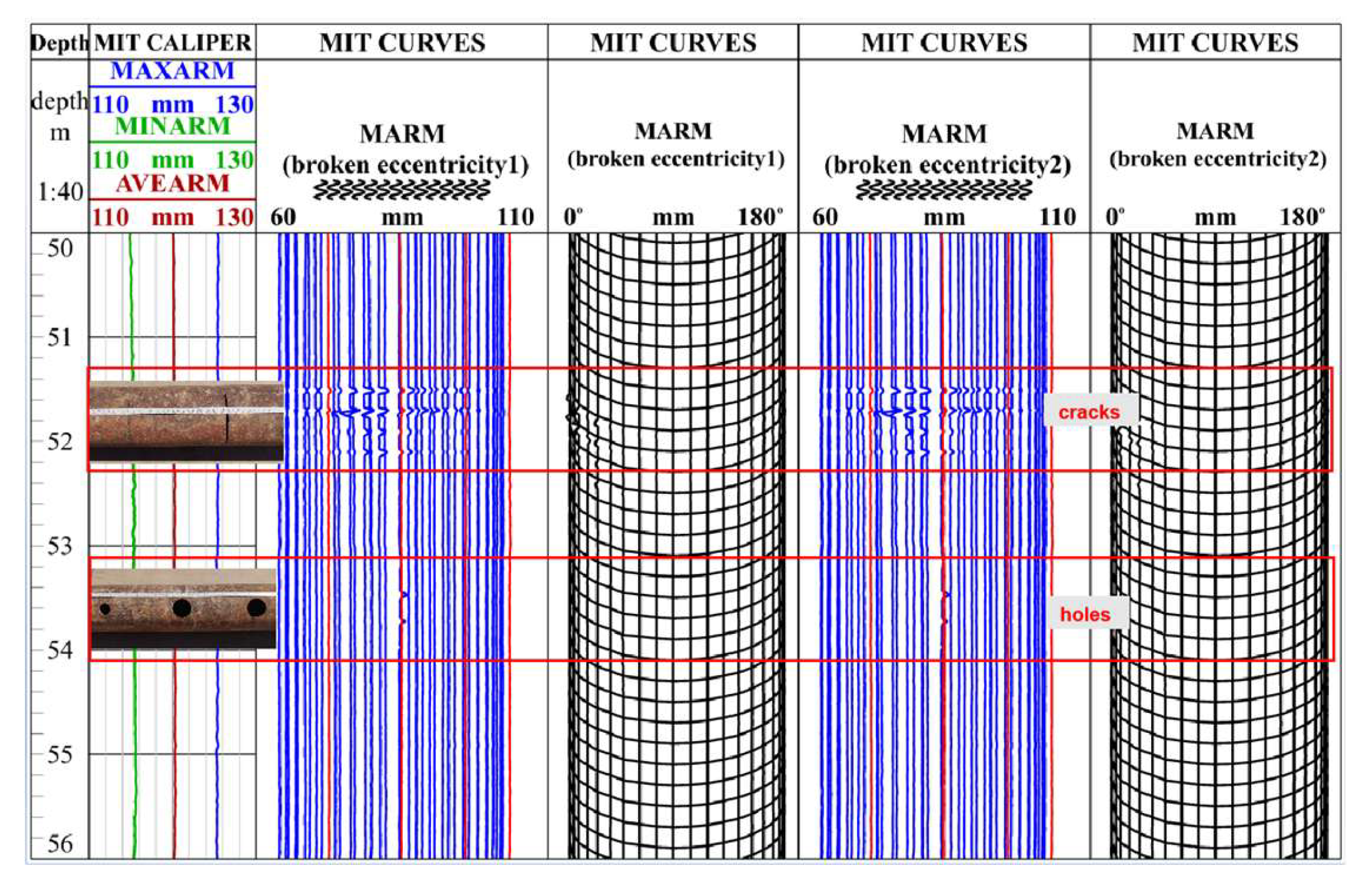
Figure 10.
Cross-sectional views of before and after eccentricity correction.
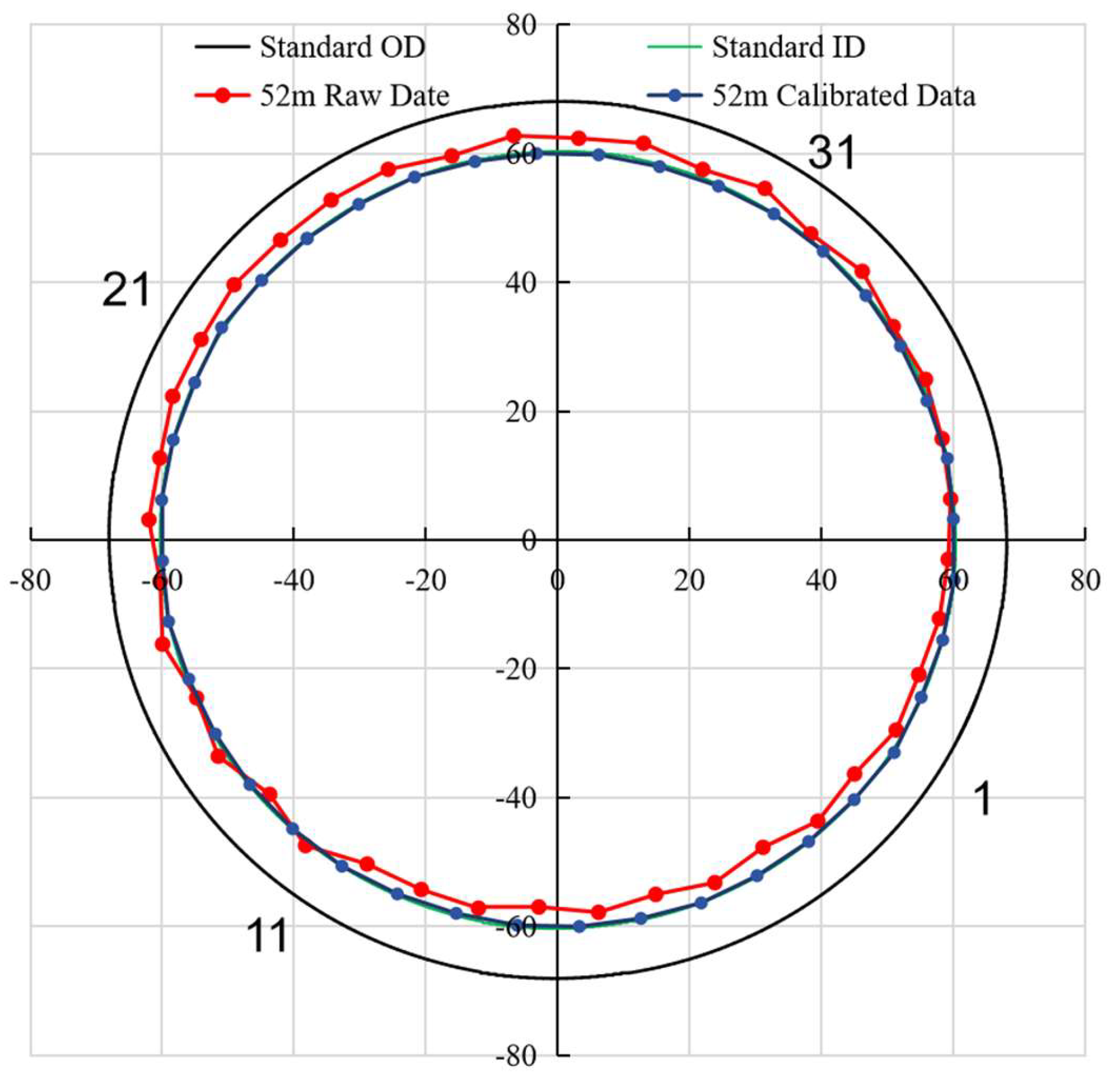
Figure 11.
Schematic diagram of the position of the instrument in the wellbore before and after the horizontal well eccentricity.
Figure 11.
Schematic diagram of the position of the instrument in the wellbore before and after the horizontal well eccentricity.
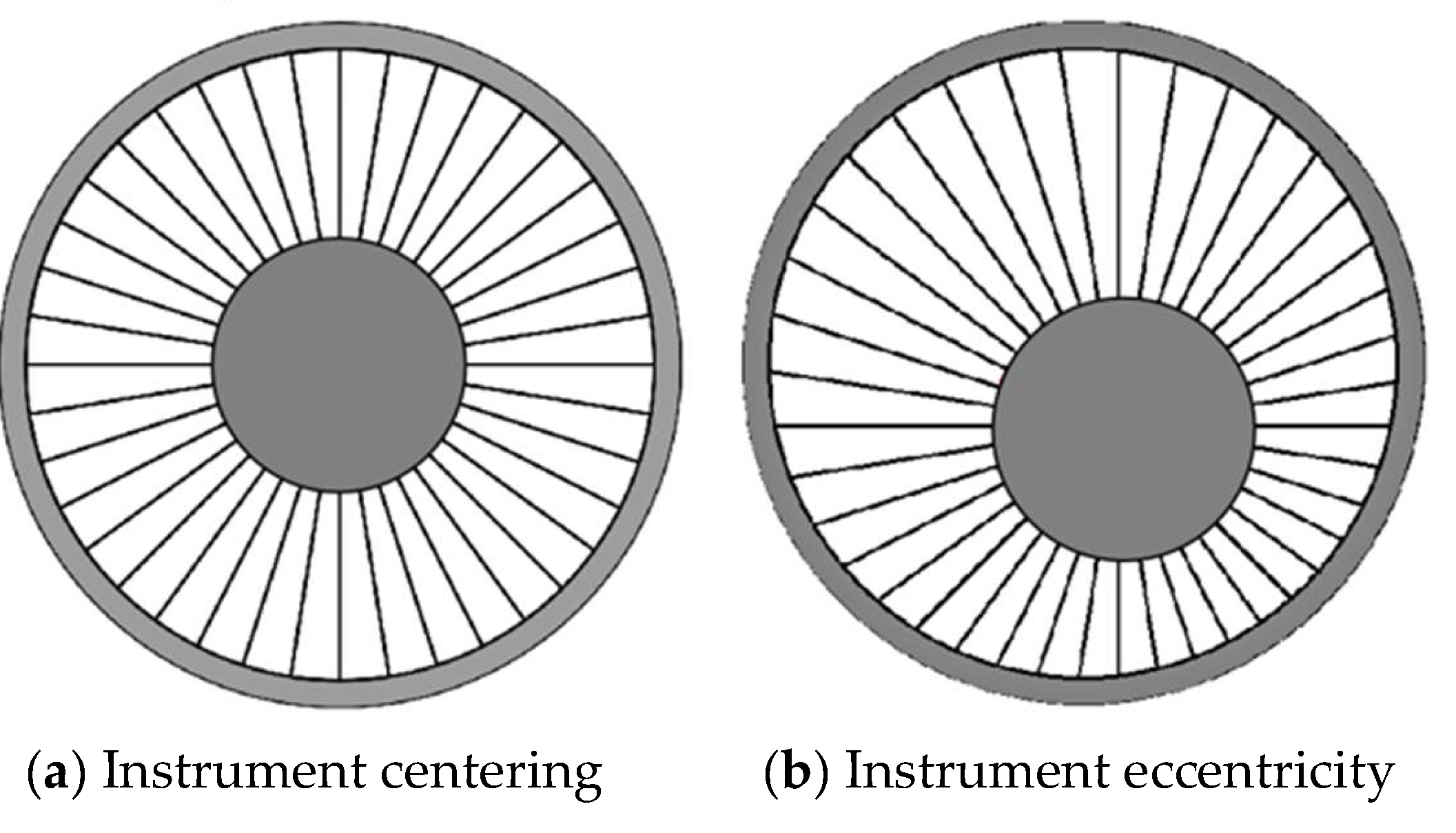
Figure 12.
Schematic of vertical deviation of the caliper logging instrument.
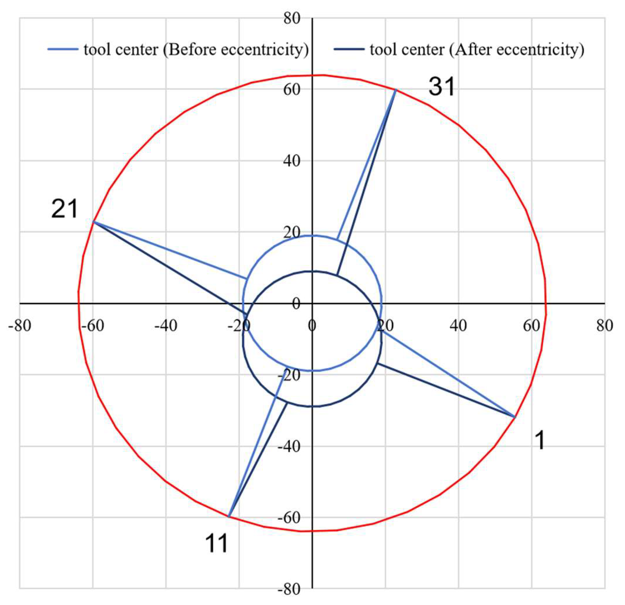
Figure 13.
Schematic of the axial and horizontal deviation of 40-arm caliper logging instrument (no damage).
Figure 13.
Schematic of the axial and horizontal deviation of 40-arm caliper logging instrument (no damage).
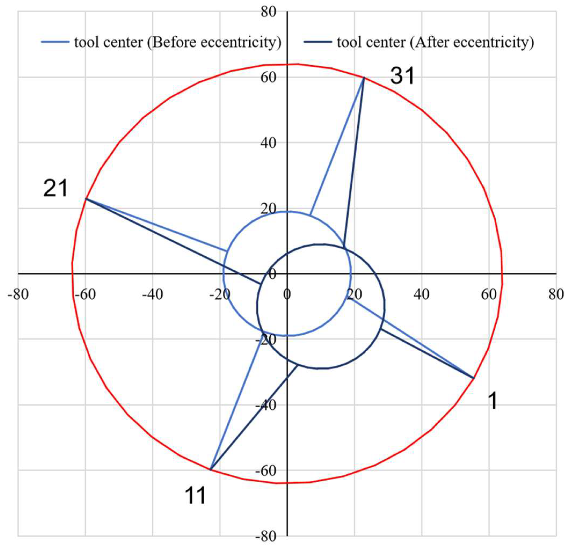
Figure 14.
Schematic diagram of axial and horizontal offset of 40-arm caliper logging instrument (broken).
Figure 14.
Schematic diagram of axial and horizontal offset of 40-arm caliper logging instrument (broken).
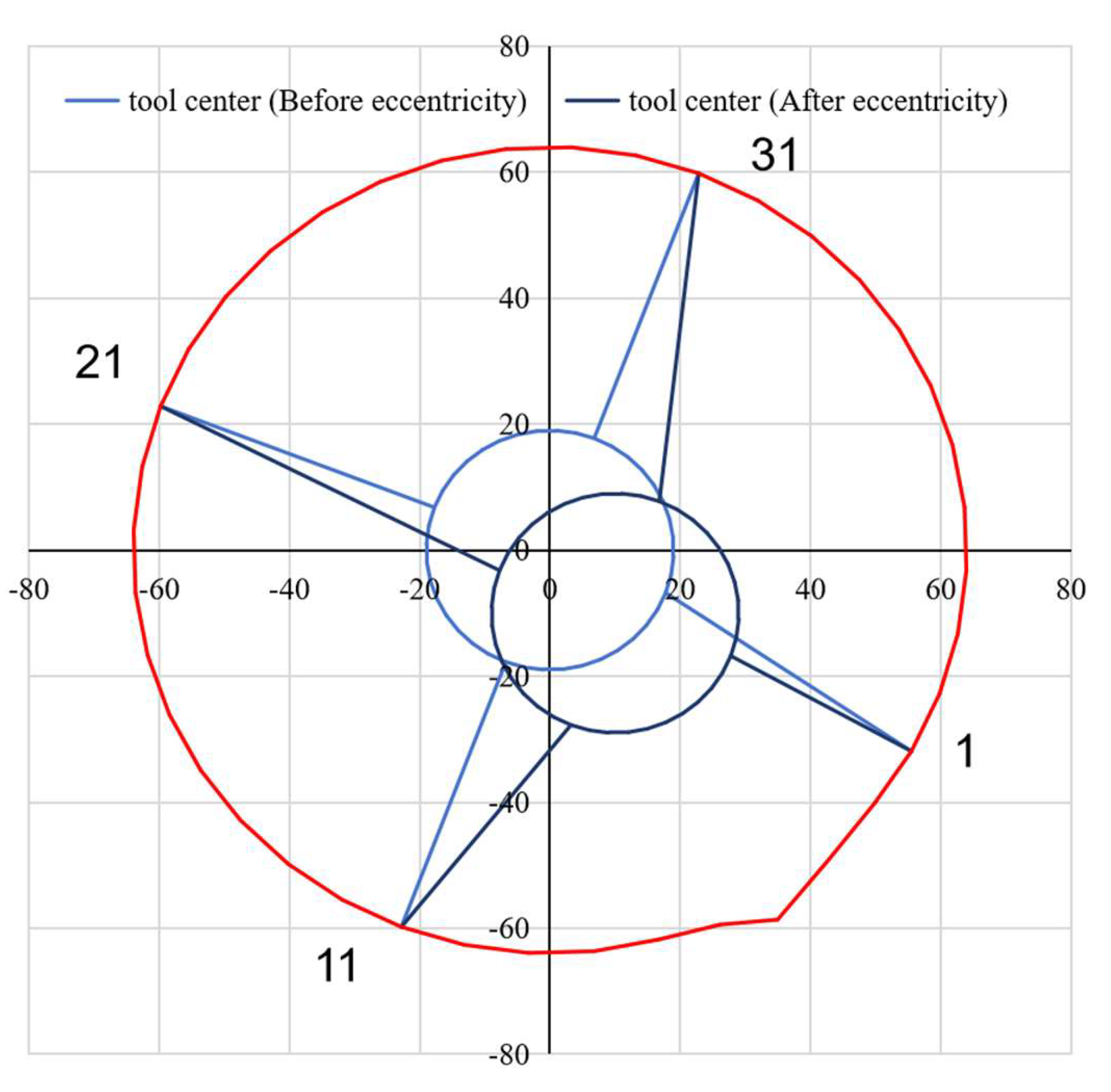
Figure 15.
Comprehensive results of various eccentric correction methods under intact casing and instrument centering conditions.
Figure 15.
Comprehensive results of various eccentric correction methods under intact casing and instrument centering conditions.
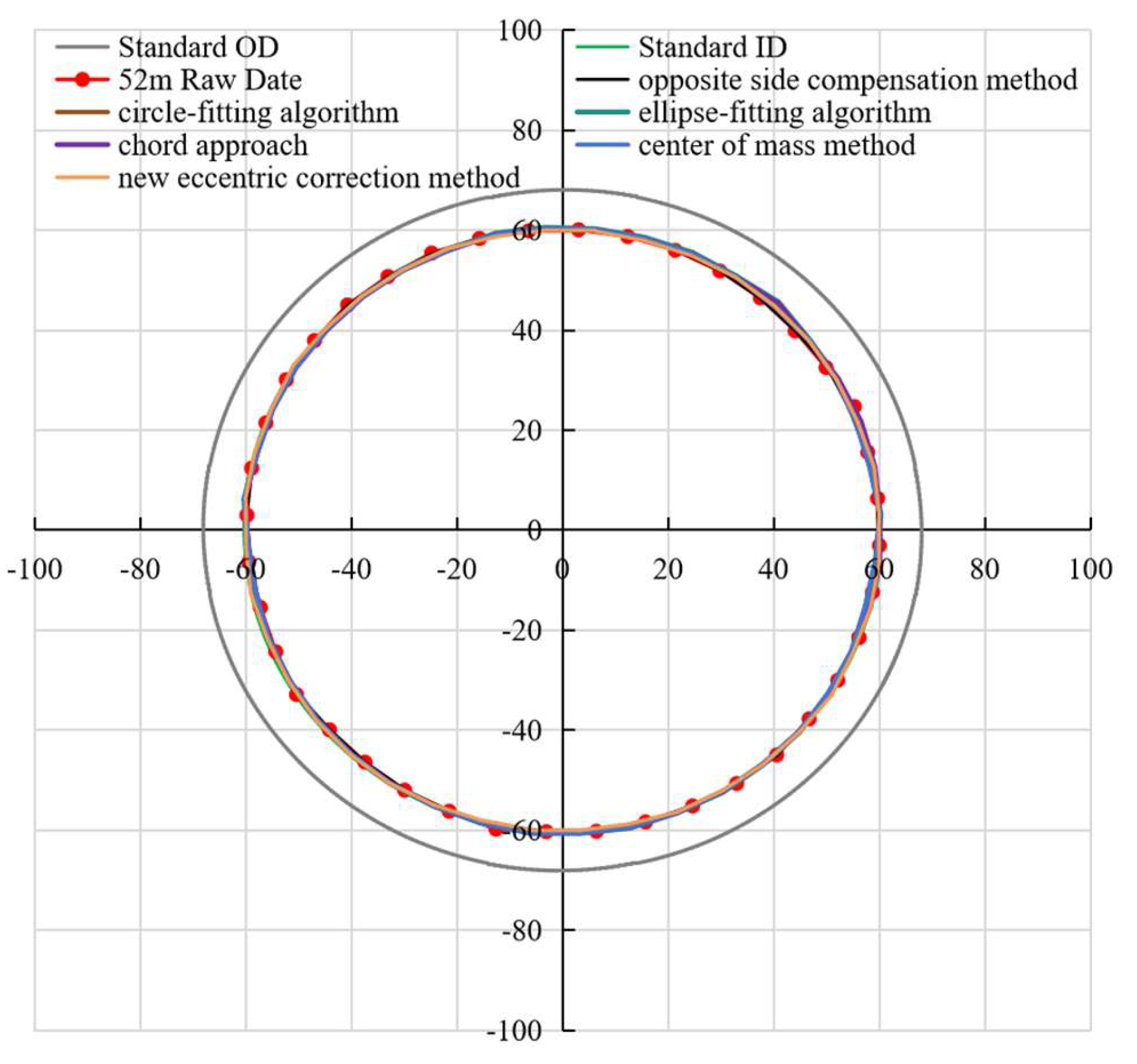
Figure 16.
Comprehensive results of various eccentric correction methods under intact casing and instrument eccentricity conditions.
Figure 16.
Comprehensive results of various eccentric correction methods under intact casing and instrument eccentricity conditions.
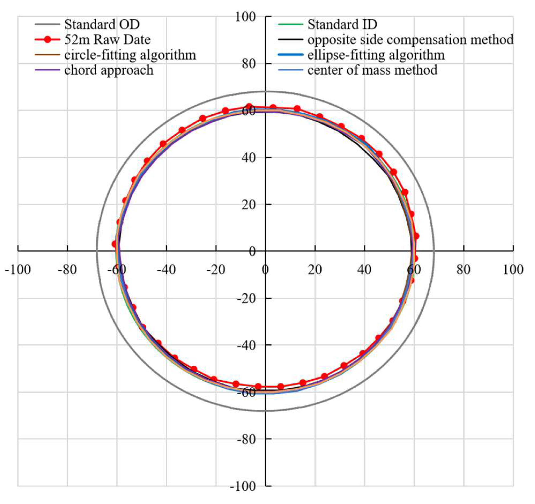
Figure 17.
Comprehensive results of various eccentric correction methods under damaged casing and instrument centering conditions.
Figure 17.
Comprehensive results of various eccentric correction methods under damaged casing and instrument centering conditions.
Figure 18.
Comprehensive results of various eccentric correction methods under damaged casing and instrument eccentricity conditions.
Figure 18.
Comprehensive results of various eccentric correction methods under damaged casing and instrument eccentricity conditions.
Figure 19.
Result diagrams of different eccentric correction methods under the scenarios of casing damage and instrument eccentricity (a–f).
Figure 19.
Result diagrams of different eccentric correction methods under the scenarios of casing damage and instrument eccentricity (a–f).
Figure 20.
Error analysis diagrams of each eccentric correction processing under the condition that casing is damaged and instrument is eccentric (a–f).
Figure 20.
Error analysis diagrams of each eccentric correction processing under the condition that casing is damaged and instrument is eccentric (a–f).
Figure 21.
Error analysis diagrams of eccentric and centered measurement methods under damaged casing and intact casing conditions (a–b).
Figure 21.
Error analysis diagrams of eccentric and centered measurement methods under damaged casing and intact casing conditions (a–b).
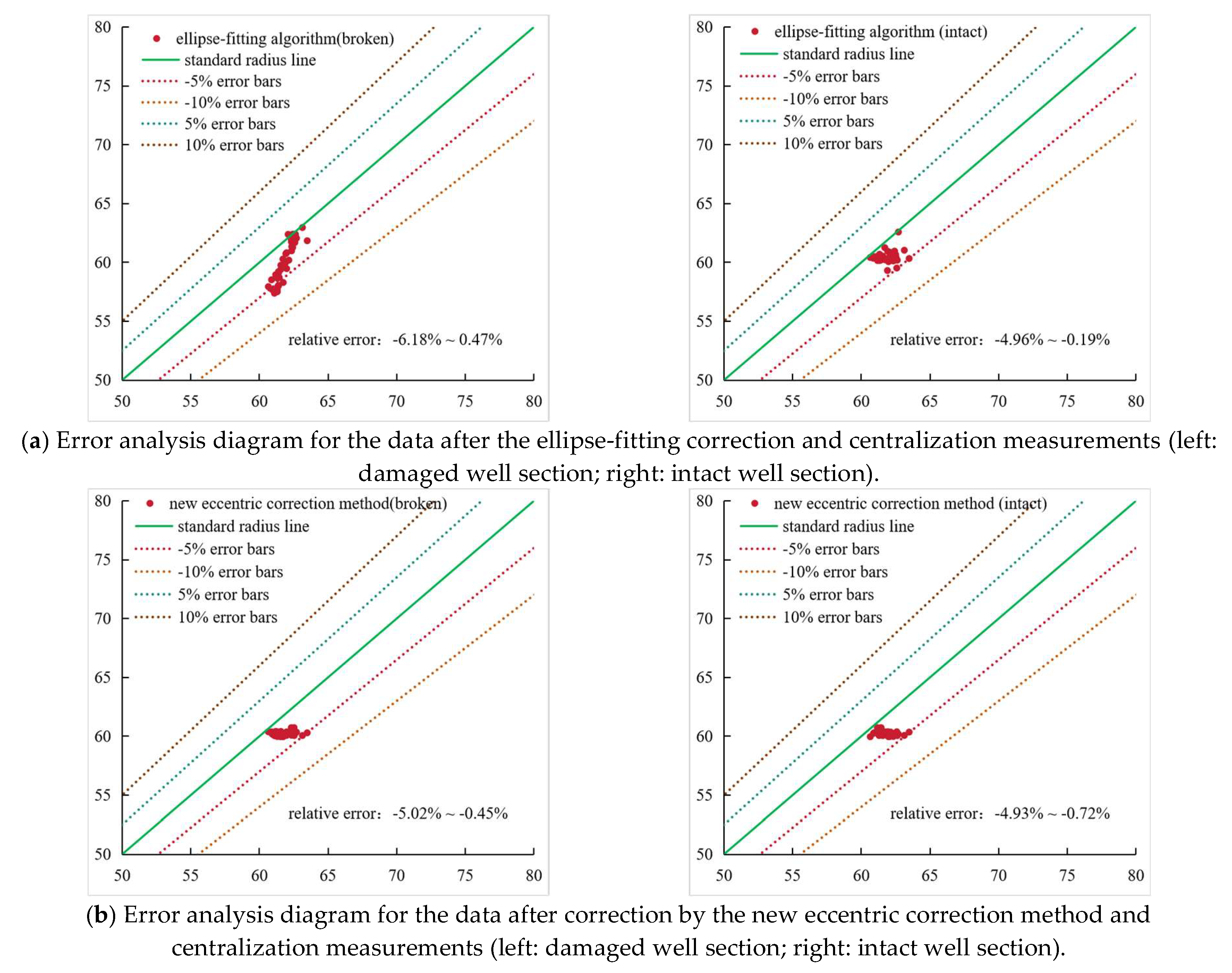
Figure 22.
3D correction diagrams of well sections before and after eccentricity correctionAuthors should discuss the results and how they can be interpreted from the perspective of previous studies and of the working hypotheses. The findings and their implications should be discussed in the broadest context possible. Future research directions may also be highlighted.
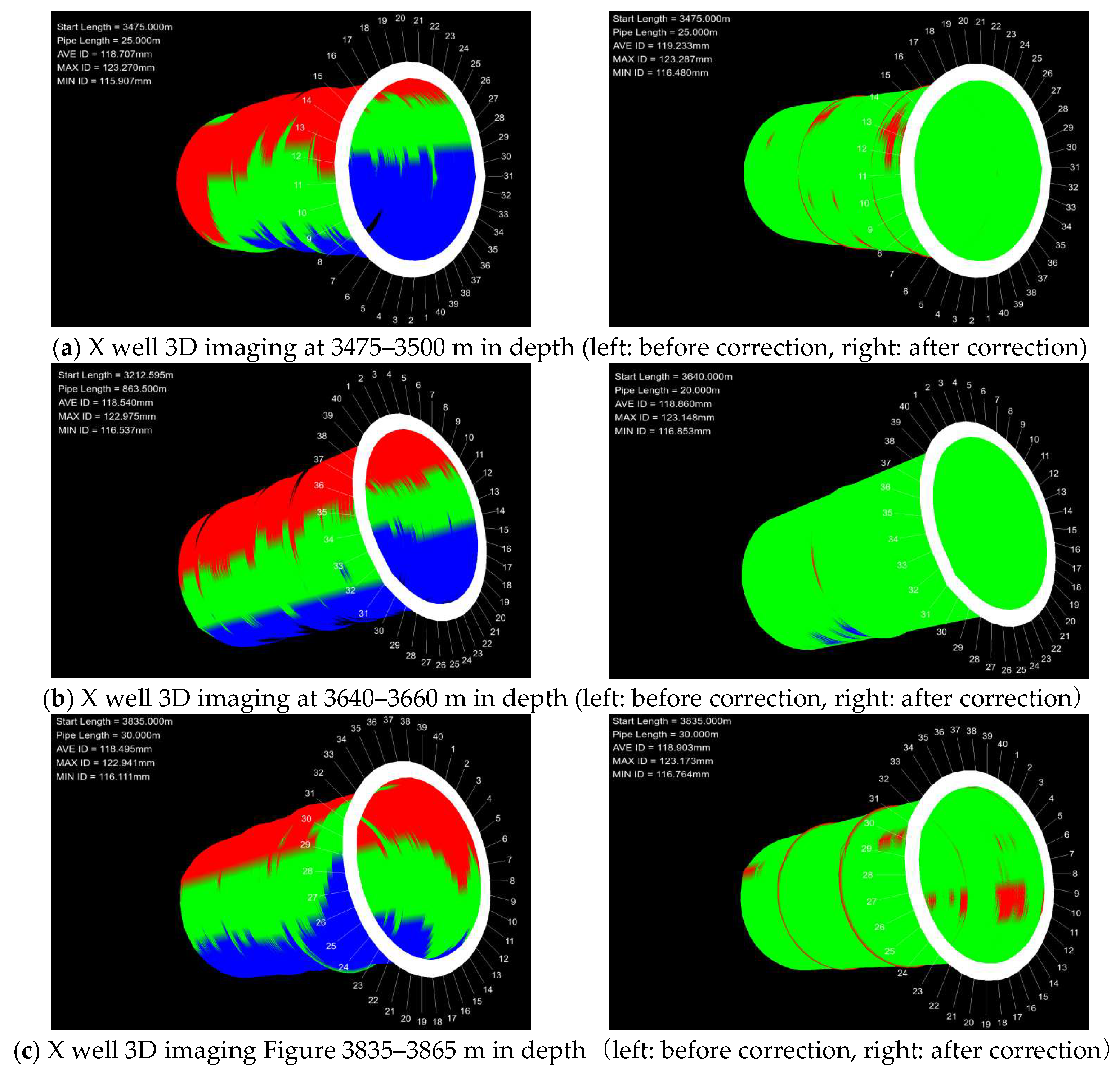

Table 1.
Comparison of existing eccentricity correction methods.
| References | Method | formulas |
|---|---|---|
| Ning, 2015 | Opposite side compensation method | |
| Bässler, 1995;Barton, 1988;Wagner et al., 2004 | Circle-fitting algorithm | |
| Lysne, 1986;Barton, 1988;Bässler, 1995;Wagner et al., 2004 | Ellipse-fitting algorithm | |
| Bässler, 1995;Barton, 1988;Wagner et al., 2004 | Center of mass method | , |
| Wagner et al., 2004;Yang et al., 2018 | Chord approach |
, |
| Yang et al.,2018 | Confined best-fit circle method |
Note: D is the case diameter, mm; r1 and r2 are the corresponding radii; (x0 , y0) is tool center; (xi, yi) is the coordinates of arms; a, b, c, d, e are the equation coefficients of the ellipse; x is equal to Ri.cosθi, y is equal to Ri.sinθi; (Ri, θi)is the borehole diameter data measured at the i-th point.; Pi is the measured caliper lengths of the individual pads; (Pi·cosθi, Pi·sinθi) are the coordinates of the arm probe; R is radius, mm.
Disclaimer/Publisher’s Note: The statements, opinions and data contained in all publications are solely those of the individual author(s) and contributor(s) and not of MDPI and/or the editor(s). MDPI and/or the editor(s) disclaim responsibility for any injury to people or property resulting from any ideas, methods, instructions or products referred to in the content. |
© 2025 by the authors. Licensee MDPI, Basel, Switzerland. This article is an open access article distributed under the terms and conditions of the Creative Commons Attribution (CC BY) license (http://creativecommons.org/licenses/by/4.0/).
Copyright: This open access article is published under a Creative Commons CC BY 4.0 license, which permit the free download, distribution, and reuse, provided that the author and preprint are cited in any reuse.


