Submitted:
04 November 2025
Posted:
06 November 2025
You are already at the latest version
Abstract
A vibration energy harvester (VEH) based on the principle of variable magnetic reluctance has been developed to enable wireless and maintenance-free power supply for condition monitoring sensors in vibrating machinery. Conventional battery or wired solutions are often impractical due to limited lifetime and high installation costs, motivating the use of vibration-based energy harvesting. The proposed VEH converts mechanical vibrations into electrical energy through the relative motion of a movable ferromagnetic core within a magnetic circuit. Unlike conventional VEH designs where the magnet is the moving element, this concept utilizes a movable ferromagnetic core in combination with a stationary pole piece for voltage induction. This configuration enables a compact and easily adjustable proof mass, as neither the coil nor the magnet need to be moved. The VEH is designed to operate effectively under excitation frequencies between 16 Hz and 50 Hz and acceleration levels from 9,81 m/s2 (equivalent to 1g) up to 98,1 m/s2 (equivalent to 10g). To ensure reliable power supply, the VEH must deliver a minimum electrical output of 0.1 mW at the lowest excitation (1g) while maintaining structural integrity. Additionally, the maximum permissible displacement amplitude of the movable core is limited to 1.15 mm to avoid mechanical damage and ensure durability over long-term operation. Coupled magnetic-transient and mechanical finite element method (FEM) simulations were conducted to analyze the system’s dynamic behavior and electrical power output across varying excitation frequencies and accelerations. A laboratory prototype was developed and tested under controlled vibration conditions to validate the simulation results. The experimental measurements confirm that the VEH achieves an electrical output of 0.166 mW at 9,81 m/s2 and 16 Hz, while maintaining the maximum allowable displacement amplitude of 1.15 mm even at 98,1 m/s2 (10g) and 50 Hz. The strong agreement between simulation and experimental data demonstrates the reliability of the coupled FEM approach. Overall, the proposed VEH design meets the defined performance targets and provides a robust solution for powering wireless sensor systems under a wide range of vibration conditions.
Keywords:
vibration energy harvesting
; finite element simulation
; condition monitoring
; variable reluctance
; electromagnetic damping
; wireless sensor systems
1. Introduction
Wireless sensor networks (WSNs) and the Internet of Things (IoT) have created a growing demand for sensor systems capable of real-time monitoring of machines and structural components [1,2,3]. Conventional power supplies for these sensors, such as batteries or wired connections, pose several challenges. Batteries often suffer from limited lifetimes, large physical dimensions, and the need for frequent replacement, which can lead to costly machine downtime [4,5]. Wired power supply systems, on the other hand, are susceptible to failures and make retrofitting sensors on existing machinery both complex and expensive.
An alternative approach is to use VEHs as autonomous power sources for sensor nodes [6]. For condition monitoring applications, VEHs typically need to provide an average electrical power between 0.1 and 1 mW [7,8]. The wireless data transmission of sensor nodes accounts for the largest portion of this power consumption [6].
Energy harvesting refers to the conversion of ambient energy into usable electrical energy. Possible ambient energy sources include light, wind, temperature gradients, motion, and machine vibrations. This enables the autonomous operation of small wireless devices such as those found in distributed sensor networks [7,8].
Most VEHs can be categorized into two main functional principles: piezoelectric [4,9,10] and electromagnetic [4,9,11,12,13,14,15,16]. Electromagnetic induction is the generation of an electric current in a conductor moving within a magnetic field. In electromagnetic VEHs, electrical energy is generated either by the relative motion between a coil and a magnet or by changes in the magnetic flux density. Permanent magnets are typically used to create the magnetic field in such systems [6].
Electromagnetic VEHs generally provide higher power outputs compared to piezoelectric VEHs [17]. Commercially available VEHs are typically designed to operate near their resonance frequency, where the conversion efficiency from mechanical to electrical energy is maximized. Consequently, they must be specifically tuned to match the excitation frequency of their intended application [7,12,13,18,19]. However, in most real-world applications, excitation vibrations exhibit non-constant and time-varying frequencies. Once the excitation frequency deviates from the VEH’s resonance, the harvested power decreases drastically. Therefore, broadening the operational frequency bandwidth of VEHs is one of the key challenges in current VEH research [8]. Increasing damping can mitigate frequency dependence to some extent [6], while electromagnetic VEHs inherently offer a wider frequency range than piezoelectric ones [17].
To enable a maintenance-free, energy-autonomous sensor system suitable for retrofitting on existing machinery, electromagnetic VEHs represent a particularly promising solution.
Objective of This Study
This work presents a novel VEH concept designed to supply wireless sensor nodes with electrical energy harvested from machine vibrations. The target excitation conditions include a wide frequency range between 16 Hz and 50 Hz and acceleration levels between and (1g to 10g). To ensure sufficient energy output even outside resonance conditions, the VEH must exhibit a broad operational frequency bandwidth.
In contrast to conventional VEH designs, where the magnet is the moving element [17], the proposed design utilizes a movable ferromagnetic core in combination with a pole piece for voltage induction. This configuration enables a compact and easily adjustable proof mass, as neither the coil nor the magnet needs to be moved. The objective of this study is to investigate the vibrational and electromagnetic behavior of the system, including their coupled interactions, using FEM simulations.
Structure of the Paper
Section 2 describes the design and working principle of the proposed VEH. Section 3 presents the coupled FEM simulations that analyze both the mechanical and electromagnetic subsystems. Section 4 details the laboratory experiments conducted to validate the simulation results, while Section 5 compares the numerical and experimental data. Finally, Section 6 discusses the findings and presents the conclusions of this study.
In this work, the term frequency refers to the mechanical excitation frequency unless explicitly stated otherwise. Electrical frequencies are always denoted as electrical frequency to ensure clear distinction between mechanical and electromagnetic phenomena. All electrical and magnetic parameters are explicitly identified as such (e.g., magnetic flux density , induced voltage , or electromagnetic force ).
2. Presentation of the VEH Concept
This chapter introduces the concept, structural design, and operating behavior of the proposed VEH. The VEH converts mechanical vibrations from its environment into electrical energy by means of electromagnetic induction.To achieve reliable and efficient energy conversion over a wide frequency range, the mechanical and electromagnetic subsystems are analyzed in detail. The following sections describe the mechanical structure, the functional behavior under axial and radial excitation, and the fundamental physical relationships governing the VEH’s performance.
2.1. Spring Types
Figure 1 shows a simplified schematic of the two disc spring types employed in the VEH.
To protect proprietary design details, the exact geometry is omitted. The figure highlights only the essential dimensions and mechanical characteristics required for understanding the subsequent analysis.
2.2. Structure of the VEH Model
Figure 2 shows the schematic structure of the proposed VEH, highlighting its main components and their spatial configuration.
Two disc springs (I) are used to provide axial and radial support for the movable core (IV). The disc springs are made of cold-rolled strip steel grade 1.4310. Two different spring geometries are available, differing in their stiffness. These geometries were developed in preliminary investigations to achieve the highest possible radial stiffness while remaining functional for large vibration amplitudes. FEM pre-studies determined the axial spring stiffness N/m for spring type 1 and N/m for spring type 2. The maximum permissible amplitude for which the springs remain functional is 1.15 mm. Spring type 1 has a mass of 14.88 g, and spring type 2 weighs 15.28 g. The outer diameter of both springs is 58 mm, and the thickness is 0.8 mm. By selecting the spring stiffness and the mass of the movable core , the natural frequency of the VEH can be adjusted accordingly. The coils (III) are dimensioned such that the ratio of their height to the total axial assembly height satisfies . VEHs with these proportions have been shown to exhibit a high energy density [17]. An aluminum connecting element (VIII) links the two halves of the core. The aluminum has a relative magnetic permeability of [20]. The air gap (IX) between the core (IV) and the pole piece (V) is kept constant at 0.8 mm for all cases. This parameter remains unchanged in both the FEM simulations and the experimental setup to ensure consistency between model and measurement.
2.3. Functional Behavior
Figure 3 shows a sectional view of the VEH in its resting position (left) and with a displacement of the vibrating part (right). The physical parameters required to describe the system behavior are indicated in the illustration and defined as follows.
The total displacement of the system is denoted by , while represents the displacement of the foundation and the relative displacement between the vibrating part and the housing.The symbol denotes the combined mass of components IV and VIII, and represents the spring constant of the disc springs (I). The electrical load connected to the coils is characterized by the load resistance , and denotes the air gap between the core and the pole piece. Figure 4 shows a sectional view of the core with all axial forces caused by axial vibrations and defined as follows
The forces acting on the core during axial motion, as illustrated in Figure 4, are defined as follows.
represents the inertial force, the damping force, and the axial spring force.The parameters , , and denote the mass, damping constant, and spring constant of the system, respectively. Considering the forces acting on the movable steel core (IV) as illustrated in Figure 3, the differential equation of motion of the VEH can be expressed as follows:
The base excitation is defined as the displacement of the housing (IX), is expressed as where is the excitation amplitude and is the excitation angular frequency. represents the axial displacement of the core (IV) and the separating element (VIII) relative to components (II), (III), (V), (VI), and (IX), and is given by [20].
The second-order term in Equation (1) represents the inertial force , which can be expressed as . Here, denotes the combined mass of the core (IV) and the separating element (VIII), and is their acceleration.
The first-order term in Equation (1) represents the damping force . This damping force consists of a mechanical component and an electromagnetic component . The variable denotes the relative velocity, and is the total damping constant, which includes both a mechanical part and an electromagnetic part .
The mechanical damping force results from the internal damping of the steel, the damping at the joints, and air resistance.
A literature value for steel fits is assumed, corresponding to a damping ratio of [21]. Using the relationship it follows that:
The electromagnetic damping force results from the voltage induced in the coils (III) and is defined by the following equation: where is the coil inductance, the coil resistance, the load resistance, and the magnetic flux. Given the maximum vibration frequency of 50 Hz, the simplification is applied. This approximation is valid for excitation frequencies up to 1000 Hz [17]. Accordingly, the electromagnetic damping constant can be expressed as:
The term in Equation (1) represents the restoring force. It consists of the axial spring force and the axial reluctance force . denotes the relative displacement and is the total spring constant of the system. It is composed of the spring constant of the mechanical spring (I), denoted as , and the coefficient of the axial magnetic force–displacement characteristic.
represents the axial spring constant of the mechanical spring. Its value is N/m for spring type 1 and N/m for spring type 2. These values were determined in preliminary studies using mechanical FEM simulations.
The parameter denotes the linearized coefficient of the magnetic force–displacement characteristic. The axial magnetic reluctance force acts on the core components (IV) and (VIII) when they are displaced by from their equilibrium position [14,15,16,17,18].
The relationship between the magnetic force and the displacement of a movable armature within an iron magnetic circuit is referred to as the magnetic force–displacement characteristic [22].
From the axial magnetic reluctance force and the relative displacement of the core, the linear coefficient of the magnetic force–displacement characteristic is determined. The value of was obtained from FEM-based preliminary investigations. Within the displacement range of to , the coefficient amounts to 9296,32 N/m.
Substituting the expression for the damping constant from Equation (4), , and the expression for the spring constant from Equation (7), , into the equation of motion (Equation (1)) yields
The natural angular frequency is derived from Equation (8) using the following relationship [20]:
The relative amplitude is determined from Equation (8) using [20]:
The term of the magnification function of the forced damped vibration can be derived from Equation (10) as
where:
The electrical power is determined as follows [17]:
Since the VEH is also operated outside its natural frequency, the output power depends primarily on the frequency ratio. By substituting and from the magnification function in Equation (11) into Equation (13), the expression for the power as a function of frequency ratio is obtained.
Figure 5 displays a sectional view of the core (IV) with the radial forces acting on it caused by the radial eccentricity.
The parameters illustrated in Figure 5 are defined as follows. denotes the radial eccentricity of the core, represents the radial reluctance force, and the radial spring force. The air gap represents the radial distance between the core (IV), the housing (II), the coil (III), and the pole piece (V). As decreases, the magnetic flux density in the magnetic circuit increases, resulting in higher electromagnetic forces [23]. A small air gap therefore leads, according to Equation (6), to a high electromagnetic damping , and according to Equation (14), to a high maximum electrical power .
However, a smaller also causes a higher radial reluctance force , which tends to displace the core from its concentric equilibrium position. The force results from the radial displacement of the core, denoted by . This radial reluctance force forms an unstable equilibrium of the core around its concentric rest position at [14,15,16,17,18].
The radial spring force of the disc spring must therefore be greater than the radial reluctance force to ensure proper operation of the VEH. It follows that:
Preliminary FEM analyses determined that the minimum air gap at which the condition in Equation (15) is satisfied is .
3. Analyses of the Dynamic and Electrical Performance of the VEH Using FEM
This chapter focuses on the detailed analysis of the dynamic and electrical behavior of the proposed VEH through coupled FEM simulations. By employing coupled magnetic transient and mechanical FEM simulations, interactions between mechanical motion and electromagnetic induction are captured accurately. These simulations form the base for understanding system responses and guiding design optimizations. The following sections will present the methodology and results of the simulation analysis, demonstrating the VEH’s capability to deliver reliable power over the specified excitation range.
3.1. Coupled Magnetic Transient and Mechanical Simulation of Relative Deflection
In this section the maximum amplitudes of the movable core under maximum excitation are investigated using magnetic transient and mechanical simulations. Based on and the permissible amplitude , the functionality of the different mass–spring combinations are determined.
3.1.1. Modeling
The simulation setup consists of a magnetically transient FEM simulation in ANSYS Maxwell. It is coupled with mechanical and electrical co-simulations. The mechanical co-simulations (a-d) are implemented in ANSYS Simplorer. Their structure, shown in Figure 6, follows the axial forces shown in Figure 4 and numerically solves the equation of motion (8). Specifically, (a) applies the base excitation , (b) implements the mechanical damping force using the damping coefficient , (c) incorporates the axial spring force with spring constant , and (d) includes the mass of core (IV) and the connecting element (VIII), enabling calculation of the inertial force . Within the Maxwell co-simulation, the axial reluctance force and the electromagnetic force are determined.
The geometry used in the magnetically transient simulation corresponds to the rotationally symmetric 2D model of the functional schematic shown in Figure 2, however without the housing and springs. In the magnetically transient simulation itself, the axial reluctance force as well as the electromagnetic force are calculated. The effects of the co-simulations (a) to (d) are visualized in Figure 7.
Housing (II), core (IV), and pole piece (V) are made from unalloyed structural steel 1.0034, with permeability defined by the B-H curve given in ANSYS. The Coil (III) is modeled as stranded copper wire ( [20]). The magnet (VI) is radially magnetized (NdFe35B35; see Table 1):
The core is axially movable. Each coil is connected to two load resistors. and represent the internal resistance of the Coils. They were measured as and . Load resistors are set to , maximizing electromagnetic damping (Eq. 8).
Mesh convergence is achieved when the reluctance force changes by less than 1%.
3.1.2. Procedure
The system is excited using . Mechanical frequency varies from 16 Hz to 50 Hz with a step size of 4.25 Hz. Amplitude corresponds to 10 g acceleration at each frequency (Table 2):
Spring constant and mass are chosen so that the expected relative amplitude (Eq. 11) remains below the amplification function’s maximum (16–50 Hz). The Time step is defined as 0.3 ms (Resulting in 50 data points for a 50 Hz cycle). The period under consideration is defined as 900 ms.
3.1.3. Result
Figure 8 shows the maximum relative amplitude versus excitation frequency. The Data points are connected using linear interpolation. The limit is marked in red; only combinations with are considered functional.
The mass-spring combinations using spring 2 with masses of 197 g, 246 g and 296 g are suitable for the VEH.
3.2. Coupled Magnetic Transient and Mechanical Simulation of Electrical Power
This section analyzes the electrical power output of the VEH via coupled magnetic transient and mechanical FEM simulations under a constant excitation of 1 g across frequencies from 16 Hz to 50 Hz. By varying the load resistance, the study identifies optimal conditions for power generation, providing insights into the VEH’s performance and guiding its design optimization.
3.2.1. Modeling
The simulation setup corresponds to that of the simulation of the maximum amplitude occurring. In this case, the excitation corresponds to the minimum value of 1 g.
3.2.2. Procedure
The system is excited using . The frequency varies between 16 Hz and 50 Hz. The amplitude is adjusted at each frequency to correspond to an excitation of 1 g.

Table 3.
Input parameters for excitation at (1g).
| Frequency (Hz) | Amplitude (mm) |
|---|---|
| 16 | 0,970 |
| 25 | 0,397 |
| 50 | 0,099 |
The load resistances and are varied between 1000 Ω, 2000 Ω, 4000 Ω, 6000 Ω, 8000 Ω, and 10,000 Ω to optimize power output.
3.2.3. Result
Figure 9 shows the average electrical power in a steady state. is plotted as a function of load resistance for excitation frequencies of 16 Hz, 25 Hz, and 50 Hz. Linear interpolation is performed between the six data points each.
Of the six discrete load resistance values, the maximum average power at 16 Hz excitation is 0.101 mW for 2000 Ω. At 25 Hz, reaches its maximum 0.257mW for 2000 Ω. At 50 Hz, the maximum is 2.026 mW for 4000 Ω.
The FEM simulations indicate that the mass-spring combination (spring 2, 296 g) is both suitable for the specified maximum amplitude and delivers at least 0.1 mW of power under minimum excitation.
4. Laboratory Tests
This chapter presents the experimental validation of the maximum relative amplitude of the VEH’s movable core for selected mass–spring combinations previously identified through FEM simulations. Using a laboratory prototype that replicates the simulation model, vibration tests are conducted under controlled sinusoidal excitations. The setup includes measurement of both the base excitation and the core’s acceleration using precision sensors, allowing determination of the relative displacement amplitudes. The experimental results are compared with simulation predictions to verify the accuracy of the modeling approach and to confirm the functionality of the investigated configurations.
4.1. Experimental Validation of Maximum Amplitude
The mass–spring combinations that exhibit a maximum amplitude below , as determined in the previous FEM analysis, are investigated.
4.1.1. Setup
The mass–spring combinations that exhibit a maximum amplitude below , as determined in the previous FEM analysis, are investigated. The coils are connected to load resistors with resistance values of , as in the simulation. The laboratory prototype shown in Figure 10 consists of the same components as the simulation model in Figure 3. The Core (IV) is equipped with additional weights, while the aluminum frame (VII) includes extra feet for mounting the prototype on the shaker.
The weights are used to vary the mass m of the core. The springs (I) are used to vary the axial spring stiffness . The test setup is shown in Figure 11.
The excitation is generated by a vibration exciter S 51010/LS-340 from TIRA GmbH. The time response of the vibrations is recorded using two acceleration sensors 3055D6 from Dytran Instruments Inc. and a data acquisition board DT9837 from PCB Synotech GmbH. A sampling rate of 50,000 samples per second is applied.
4.1.2. Procedure
Acceleration sensor b is attached to the mounting plate of the vibration exciter and measures the excitation acceleration . Acceleration sensor a is mounted to the movable core of the laboratory prototype and measures the total acceleration . The relative acceleration is obtained from the difference between the time signals of sensors a and b, from which the relative amplitude is subsequently determined. The sinusoidal displacement excitations correspond to those listed in Table 1.
4.1.3. Result
Figure 12 shows the maximum relative amplitude in steady-state conditions as a function of the excitation frequency. Between the nine measurement points for each mass–spring combination, linear interpolation is applied. The red line indicates the maximum permissible relative amplitude . Only mass–spring combinations below are suitable for the VEH.
The FEM results were confirmed. The mass-spring combinations of spring 2) with 197 g, 246 g, and 296 g are suitable for operation.
4.2. Experimental Validation for Power Delivery
In this section, the electrical power output of the movable core under minimal excitation is investigated through laboratory experiments. The experiment serves to validate the FEM simulations of the maximum electrical power . The investigation is carried out using the same mass–spring combination as in the simulation. According to Equation (7), mass–spring combinations with a higher mass-to-axial-stiffness ratio provide greater electrical power output. Therefore, the combination consisting of Spring 2 and a mass of 296 g is examined.
4.2.1. Setup
The laboratory prototype is identical to the one used in Section 4.1. The experimental setup is shown in Figure 13.
In contrast to the setup in Section 4.1, the voltages and across the load resistors and are measured instead of the accelerations and . The time signals of and are recorded using the USB-6000 data acquisition device from National Instruments at a sampling rate of 10,000 samples per second.
4.2.2. Procedure
The mean electrical power is calculated from the time signals of and and the corresponding load resistances. The sinusoidal displacement excitations and the resistance values and are identical to those used in Section 2.7.
4.2.3. Result
Figure 14 shows the mean electrical power in the steady-state condition as a function of the load resistance for excitation frequencies of 16 Hz, 25 Hz, and 50 Hz. Linear interpolation is applied between the six measurement points for each excitation frequency.
At an excitation of 16 Hz, the maximum mean power is at a load resistance of . At 25 Hz, the maximum value is at , and at 50 Hz, it reaches at .
The FEM simulations indicate that the mass–spring combination consisting of Spring 2 and 296 g is suitable for operation under maximum excitation and provides at least 0.1 mW of electrical power under minimal excitation.
4. Discussion
The novel VEH concept successfully met the design requirements regarding maximum amplitude and power output through targeted parameter adjustments. By optimizing the spring stiffness , core mass , air gap length , and load resistance , both the amplitude limitation and the power generation objectives were achieved. The laboratory experiments confirmed the FEM simulation results, showing consistent behavior between simulation and measurement. The minimum generated power of meets the current design requirements for operation under low excitation conditions. Further optimization will aim to increase this minimum power level. Reducing the air gap increases the magnetic reluctance force and thus the achievable power output; however, a smaller air gap also requires a precise radial guidance of the moving core to avoid instability due to eccentricity. Future work will therefore focus on optimizing the magnetic flux path, applying progressive spring characteristics, and evaluating advanced magnetic and structural materials to improve both efficiency and long-term stability of the VEH system.
5. Conclusions
This study presented the design, simulation, and experimental validation of a VEH based on the principle of variable magnetic reluctance. The aim was to design an autonomous power source for wireless sensor systems in machine condition monitoring, capable of reliable operation under varying excitation conditions. Coupled magnetic–transient and mechanical FEM simulations were used to investigate the interaction between magnetic forces, mechanical displacement, and induced voltage. The simulation results were confirmed by laboratory measurements, showing close agreement in both displacement and electrical power output. The VEH provides a minimum electrical power of 0.166 mW at and 16 Hz, while the maximum permissible amplitude of 1.15 mm is not exceeded even at and 50 Hz. These results demonstrate that the design meets the defined requirements for energy supply and mechanical stability. The study also shows that coupled multiphysics simulation is a suitable tool for predicting the performance of electromagnetic energy harvesters. Further work will focus on increasing the energy output through optimization of the air gap. Therefore, the use of progressive spring elements and alternative magnetic materials as well as a magnetic bearing will be considered. In addition, integrating adaptive power management and wireless communication electronics will be key for future applications in fully autonomous sensor systems.
References
- Díez, P.L.; Gabilondo, I.; Alarcón, E.; Moll, F. A Comprehensive Method to Taxonomize Mechanical Energy Harvesting Technologies. IEEE Int. Symp. Circuits Syst. 2018, 1–5. [Google Scholar] [CrossRef]
- Feng, Y.; Lin, D.; Huizong, Y.; Peilin, H. Magnetic and Electric Energy Harvesting Technologies in Power Grids: A Review. Sens 2020, 20, 1496. [Google Scholar] [CrossRef]
- Fraga-Lamas, P.; Fernández-Caramés, T.M.; Castedo, L. Towards the Internet of Smart Trains: A Review on Industrial IoT-Connected Railways. Sensors 2017, 17, 1457. [Google Scholar] [CrossRef]
- Maroofiazar, R.; Farzam, F. A Hybrid Vibration Energy Harvester: Experimental Investigation, Numerical Modeling, and Statistical Analysis. J Vib Eng Technol 2022. [Google Scholar] [CrossRef]
- Kuang, Y.; Chew, Z.J.; Ruan, T.; Zhu, M. Magnetic field energy harvesting from current-carrying structures: Electromagnetic-circuit coupled model, validation and application. IEEE Access 2021, 9, 46280–46291. [Google Scholar] [CrossRef]
- Beeby, S.; Tudor, M.; White, N. Energy harvesting vibration sources for microsystems applications. Meas Sci Technol 2006, 17, 175–195. [Google Scholar] [CrossRef]
- Waterbury, A.; Wright, P. Vibration energy harvesting to power condition monitoring sensors for industrial and manufacturing equipment. J Mech Eng Sci 2012, 227, 1187–1202. [Google Scholar] [CrossRef]
- Niell, E.; Alper, E. Advances in Energy Harvesting Methods; Springer Science+Business Media: New York, 2013. [Google Scholar] [CrossRef]
- Zhua, D.; Roberts, S.; Tudor, M.; Beebya, S. Design and experimental characterization of a tunable vibration-based electromagnetic micro-generator. Sens Actuator A Phys 2010, 158, 284–293. [Google Scholar] [CrossRef]
- Kim, H.S.; Kim, J.H.; Kim, J. A Review of Piezoelectric Energy Harvesting Based on Vibration. Int J Precis Eng Manuf 2011, 12, 1129–1141. [Google Scholar] [CrossRef]
- Li, Z.; Zhou, S.; Yang, Z. Recent progress on flutter-based wind energy harvesting. Int J Mech Sci 2022, 2, 82–98. [Google Scholar] [CrossRef]
- Ayala-Garcia, L.; Mitcheson, P.; Yeatman, E. Magnetic tuning of a kinetic energy harvester using variable reluctance. Sens Actuator A Phys 2013, 189, 266–275. [Google Scholar] [CrossRef]
- Zuyao, W.; Huirong, F.; Hu, D.; Liqun, C. Parametric Infuence on Energy Harvesting of Magnetic Levitation Using Harmonic Balance Method. J Vib Eng Technol 2019, 7, 543–549. [Google Scholar] [CrossRef]
- Di Dio, V.; Franzitta, V.; Milone, D.; Pitruzzella, S.; Trapanese, M.; Viola, A. Design of Bilateral Switched Reluctance Linear Generator to Convert Wave Energy: Case Study in Sicily. Adv Mat Res 2013, 863, 1694–1698. [Google Scholar] [CrossRef]
- Gong, Y.; Wang, S.; Xie, Z.; Zhang, T.; Chen, W.; Lu, X. Self-powered Wireless Sensor Node for Smart Railway Axle Box bearing via a Variable Reluctance Energy Harvesting System. IEEE Trans Instrum Meas 2021, 70, 1–11. [Google Scholar] [CrossRef]
- Sun, K.; Liu und X, G.Q. No-load Analysis of Permanent Magnet Spring Nonlinear Resonant Generator for Human Motion Energy Harvesting. Appl Mech Mater 2011, 130, 2778–2782. [Google Scholar] [CrossRef]
- Priya, S.; Inman, D. J. Energy Harvesting Technologies, Electromagnetic Energy Harvesting. Springer Science+Business Media, LLC, 2009. [Google Scholar] [CrossRef]
- Ghouli, Z.; Litak, G. Efect of High Frequency Excitation on a Bistable Energy Harvesting System. J Vib Eng Technol 2022, 11, 99–106. [Google Scholar] [CrossRef]
- Mangalasseri, A.S.; Mahesh, V.; Mukunda, S.; Mahesh, V. Vibration Based Energy Harvesting Characteristics of Functionally Graded Magneto Electro Elastic Beam Structures Using Lumped Parameter Model. J Vib Eng Technol 2022, 10, 1705–1720. [Google Scholar] [CrossRef]
- Edwards, T.C.; Steer, M.B. Appendix B: Material Properties, Foundations for Microstrip Circuit Design IEEE, 635-642. [CrossRef]
- Link, M. Finite Elemente in der Statik und Dynamik 4., korrigierte Auflage, Springer Vieweg. [CrossRef]
- Bassani, R.; Villani, S. Passive magnetic bearings: the conic-shaped bearing. Proc IME J J Eng Tribol 1999, 213, 151–161. [Google Scholar] [CrossRef]
- Bassani, R.; Ciulli, E.; Di Puccio, F.; Musolino, A. Study of Conic Permanent Magnet Bearings. Meccanica 2001, 36, 745–754. [Google Scholar] [CrossRef]
- Schweitzer, G. Active magnetic bearings - chances and limitations. International Conference on Rotor Dynamics 2002, 6, 1–14. [Google Scholar]
- Marinescu, M. Elektrische und magnetische Felder, Der magnetische Kreis, Springer Berlin. 2009. [Google Scholar] [CrossRef]
- Knaebel, M.; Jäger, H.; Mastel, R. Technische Schwingungslehre Erzwungene Schwingungen von Systemen mit einem Freiheitsgrad mit Dämpfung, Springer Vieweg. 2013. [Google Scholar] [CrossRef]
- Bassani, R.; Earnshaw, R. 1805–1888) and Passive Magnetic Levitation. Meccanica 2006, 41, 375–389. [Google Scholar] [CrossRef]
- Bassani, R. Levitation of passive magnetic bearings and systems. Tribol Int 2006, 39, 963–970. [Google Scholar] [CrossRef]
Figure 1.
Overview of Spring Types.
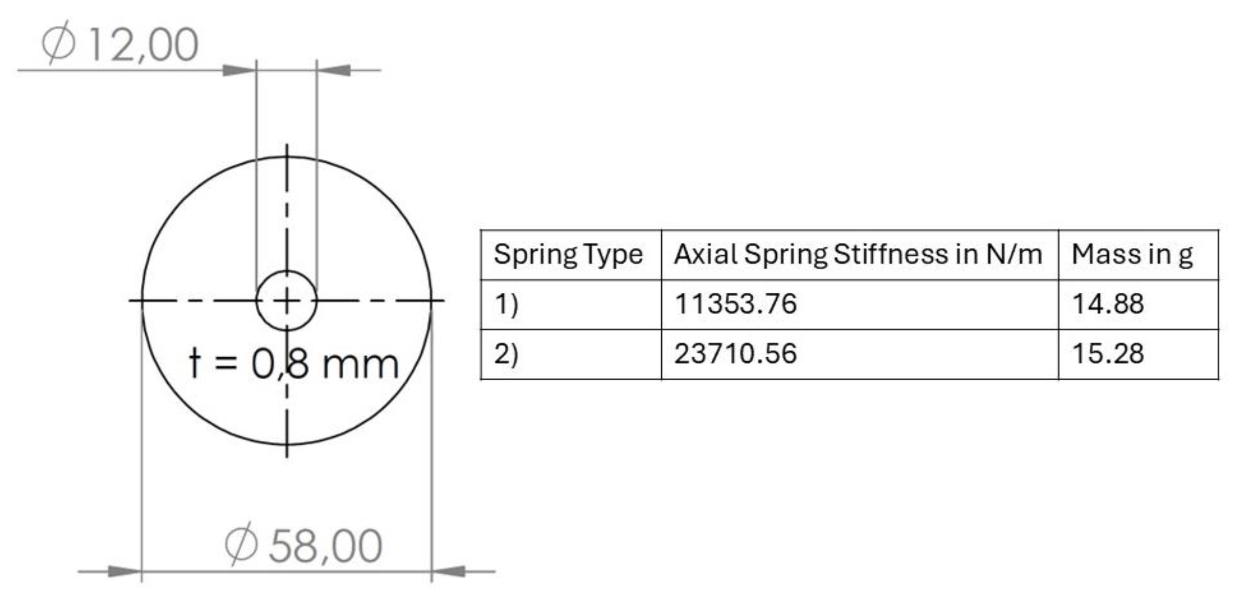
Figure 2.
VEH-Model.
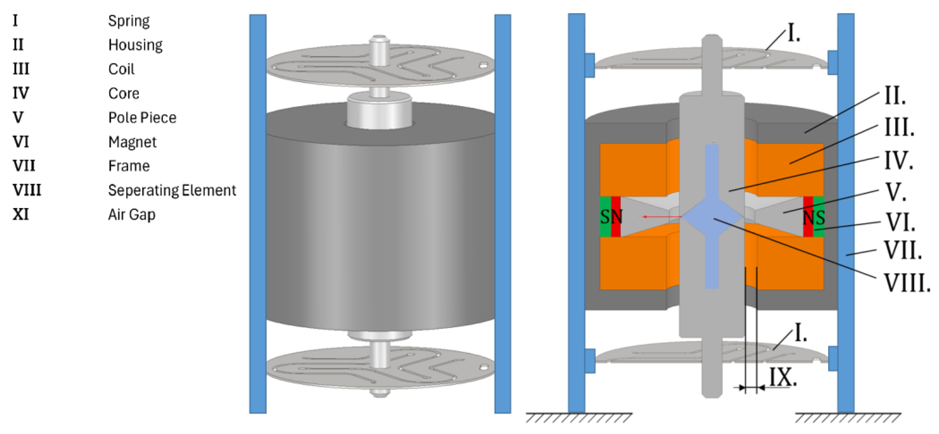
Figure 3.
Sectional view of the functional prototype with indicated physical quantities.

Figure 4.
Sectional view of the core and the forces considered during axial motion.
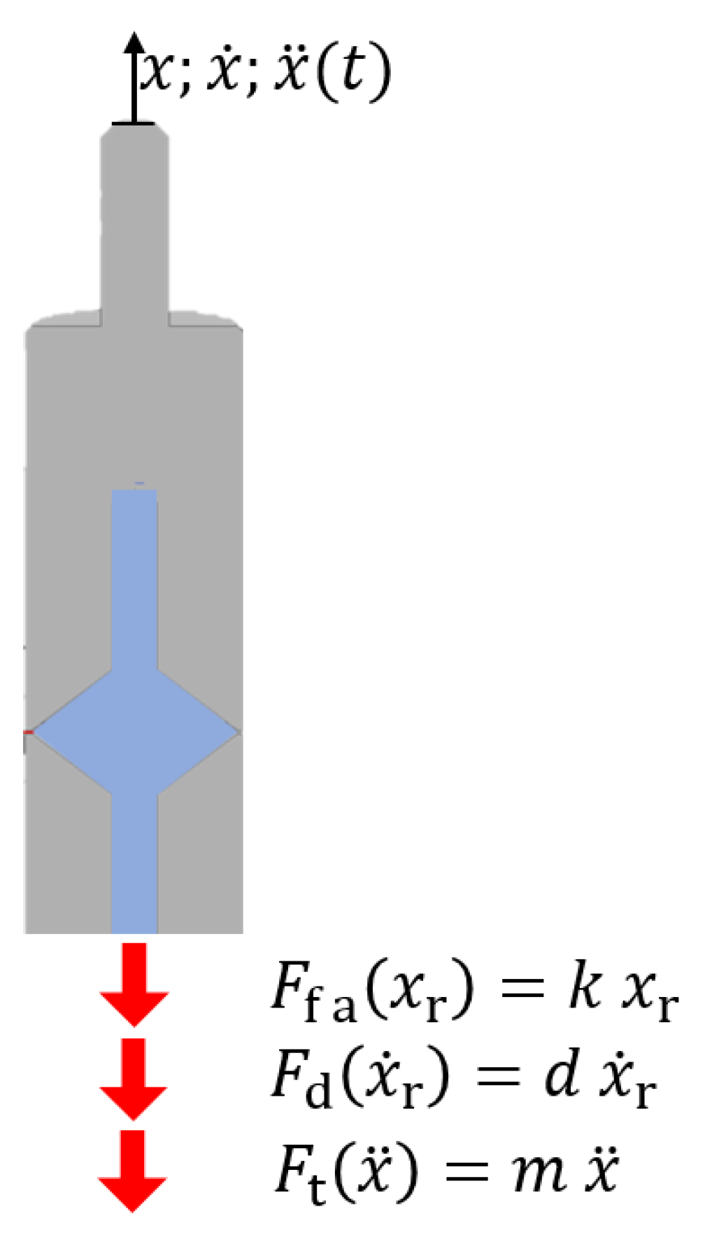
Figure 5.
Sectional view of the core and the forces caused by eccentric displacement from its equilibrium position.
Figure 5.
Sectional view of the core and the forces caused by eccentric displacement from its equilibrium position.
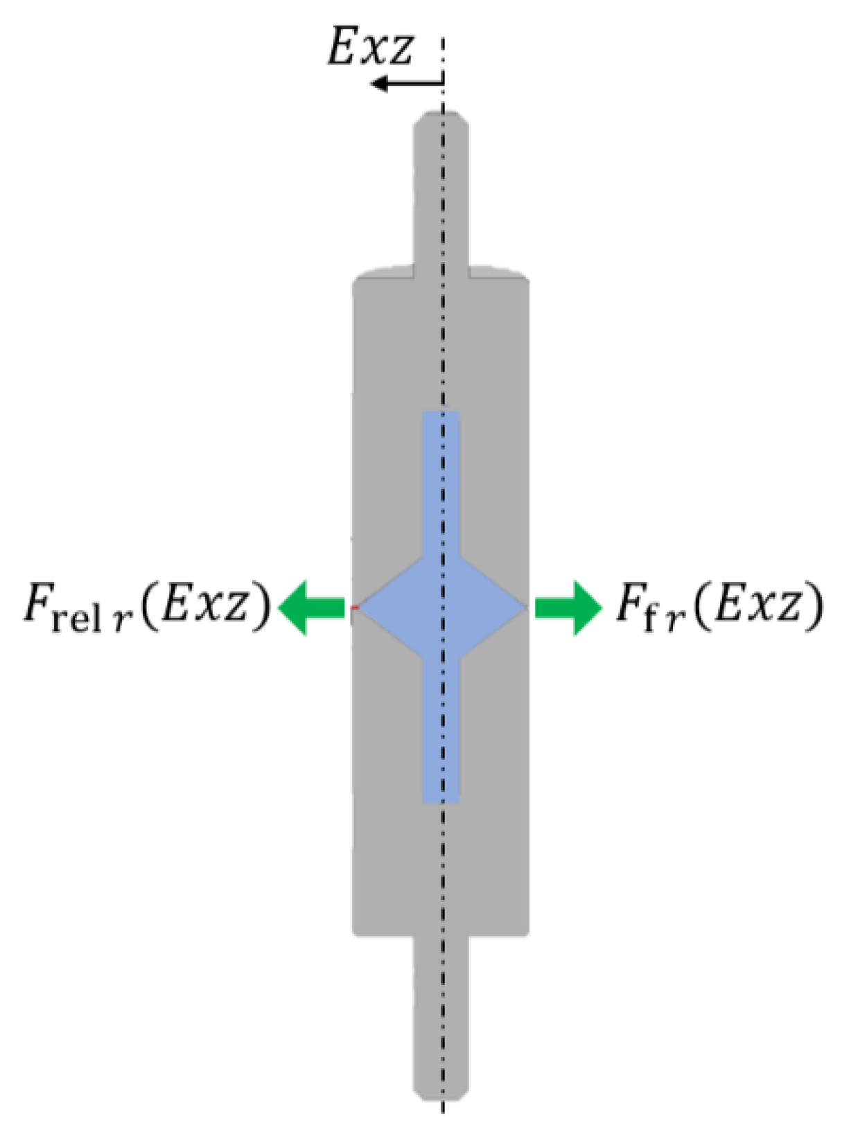
Figure 6.
Setup for Maxwell co-simulations.
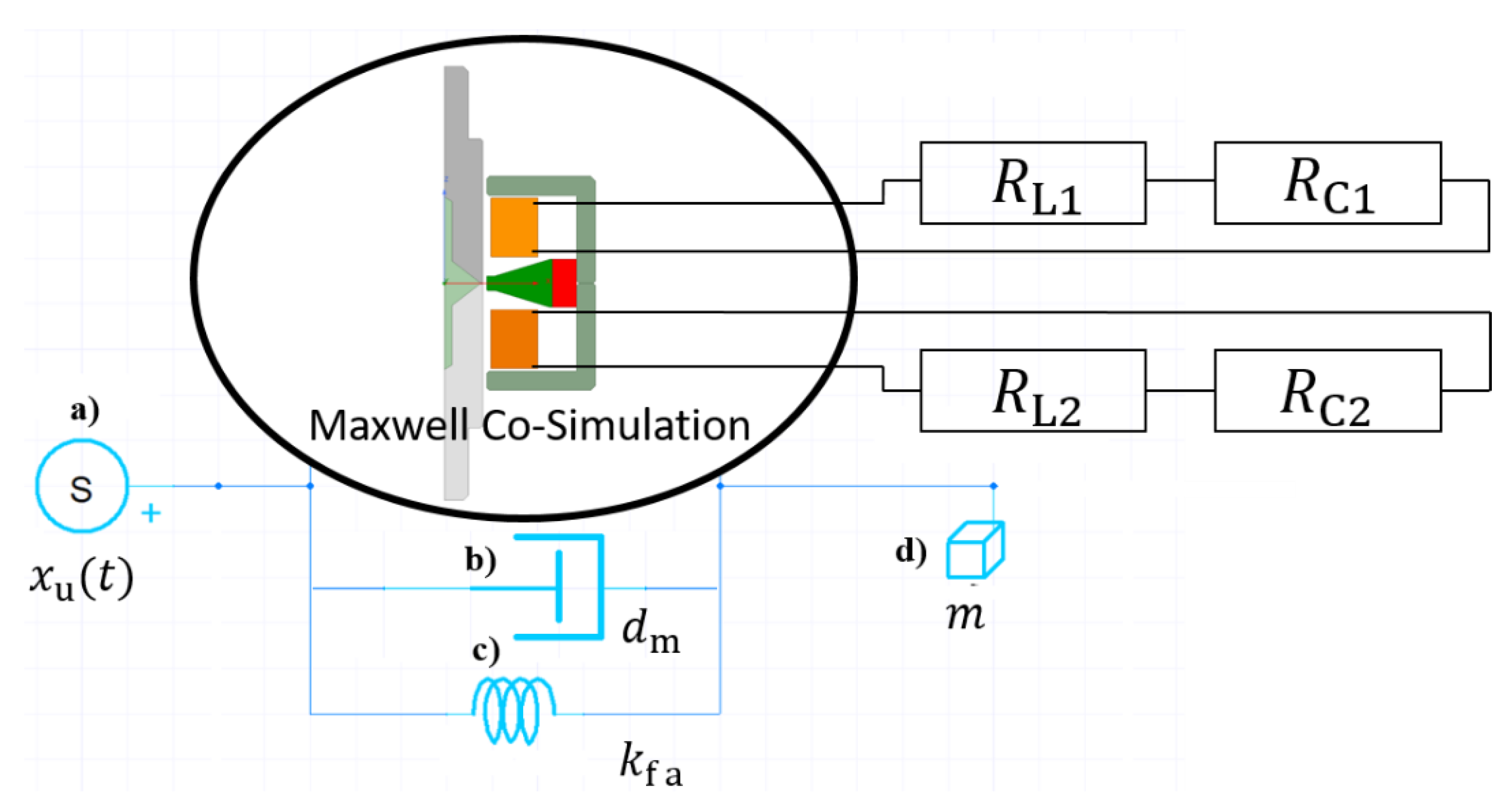
Figure 7.
Geometry of the magnetic transient simulation (co-simulation influences in red).
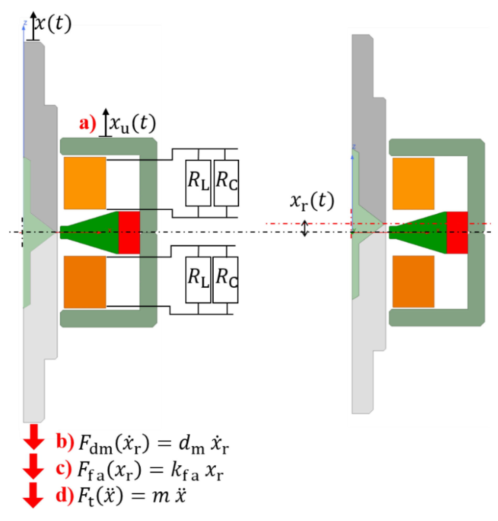
Figure 8.
Maximum relative amplitude of different mass-spring combinations.
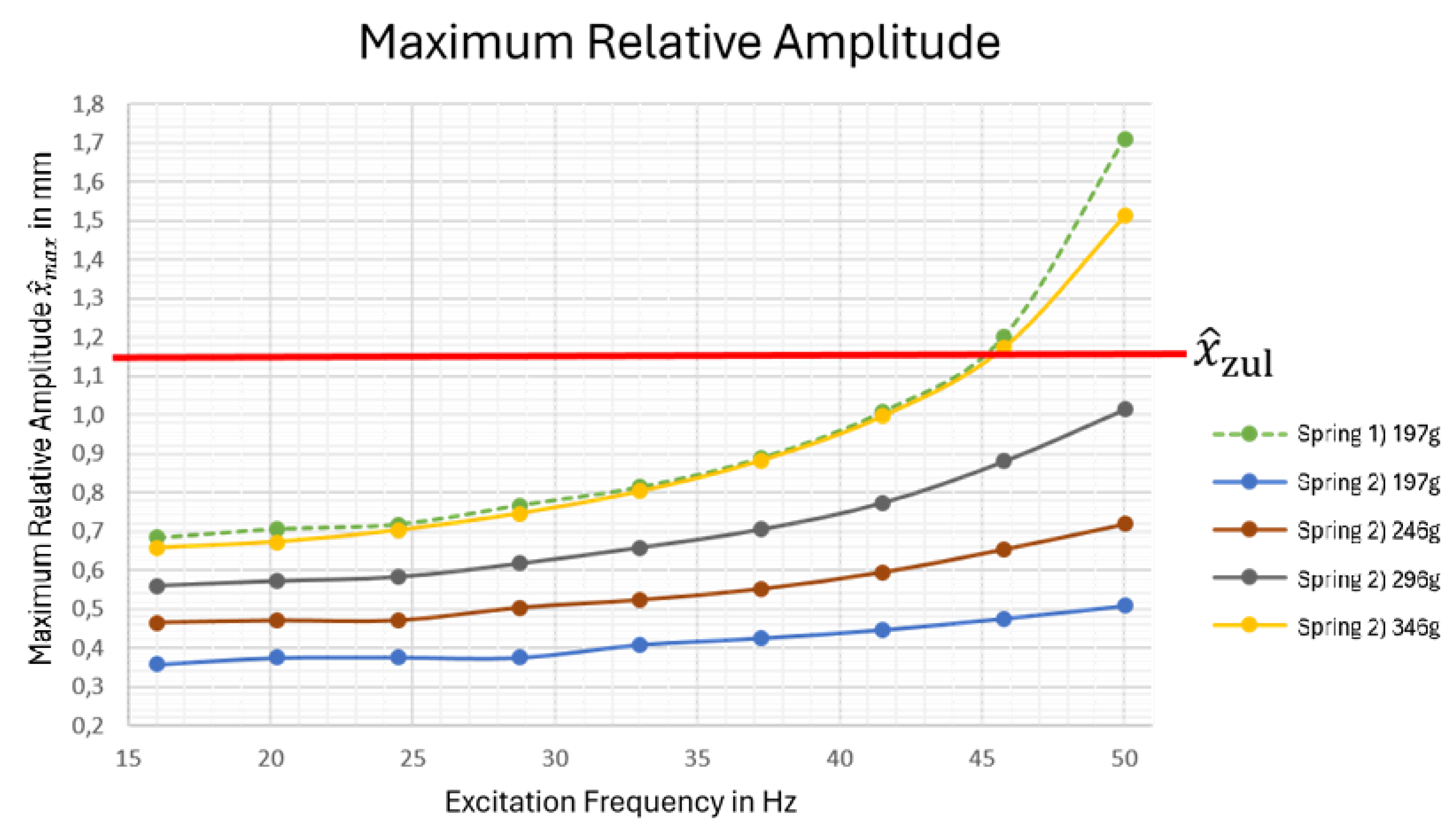
Figure 9.
Power Output under Varying Electrical Load and Frequency.
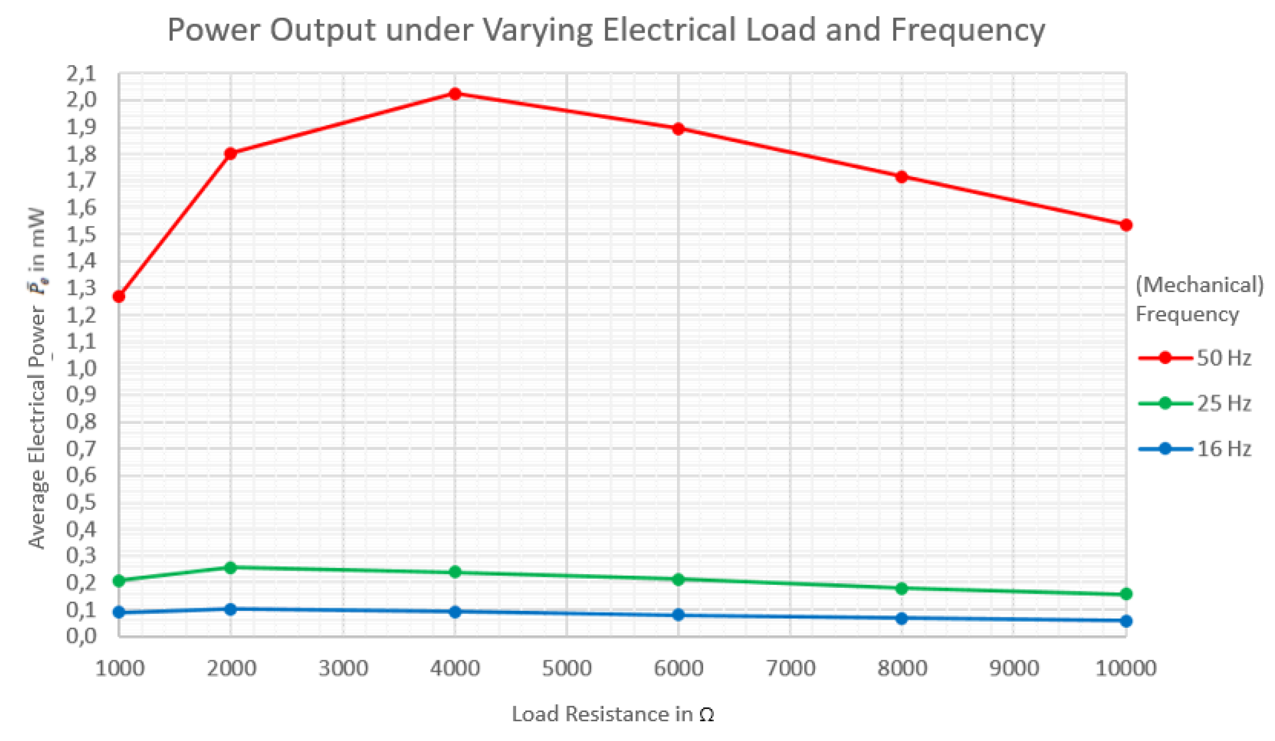
Figure 10.
Laboratory model assembly with exploded view.
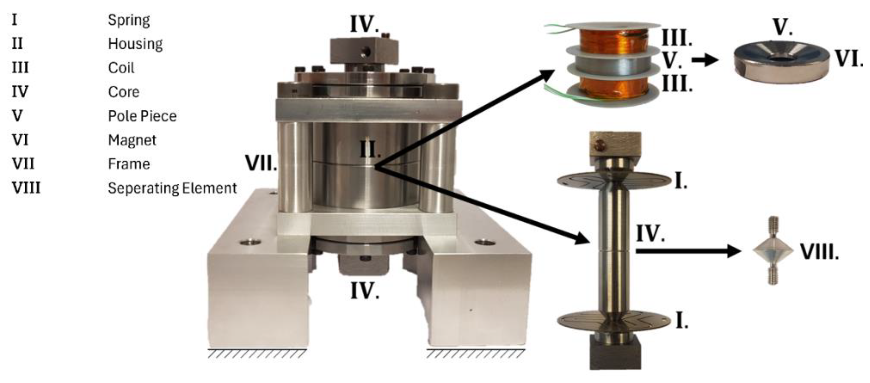
Figure 11.
Experimental setup showing the laboratory prototype, vibration exciter, acceleration sensors (a and b), load resistors ( und ), and the data acquisition board connected to the sensors.
Figure 11.
Experimental setup showing the laboratory prototype, vibration exciter, acceleration sensors (a and b), load resistors ( und ), and the data acquisition board connected to the sensors.
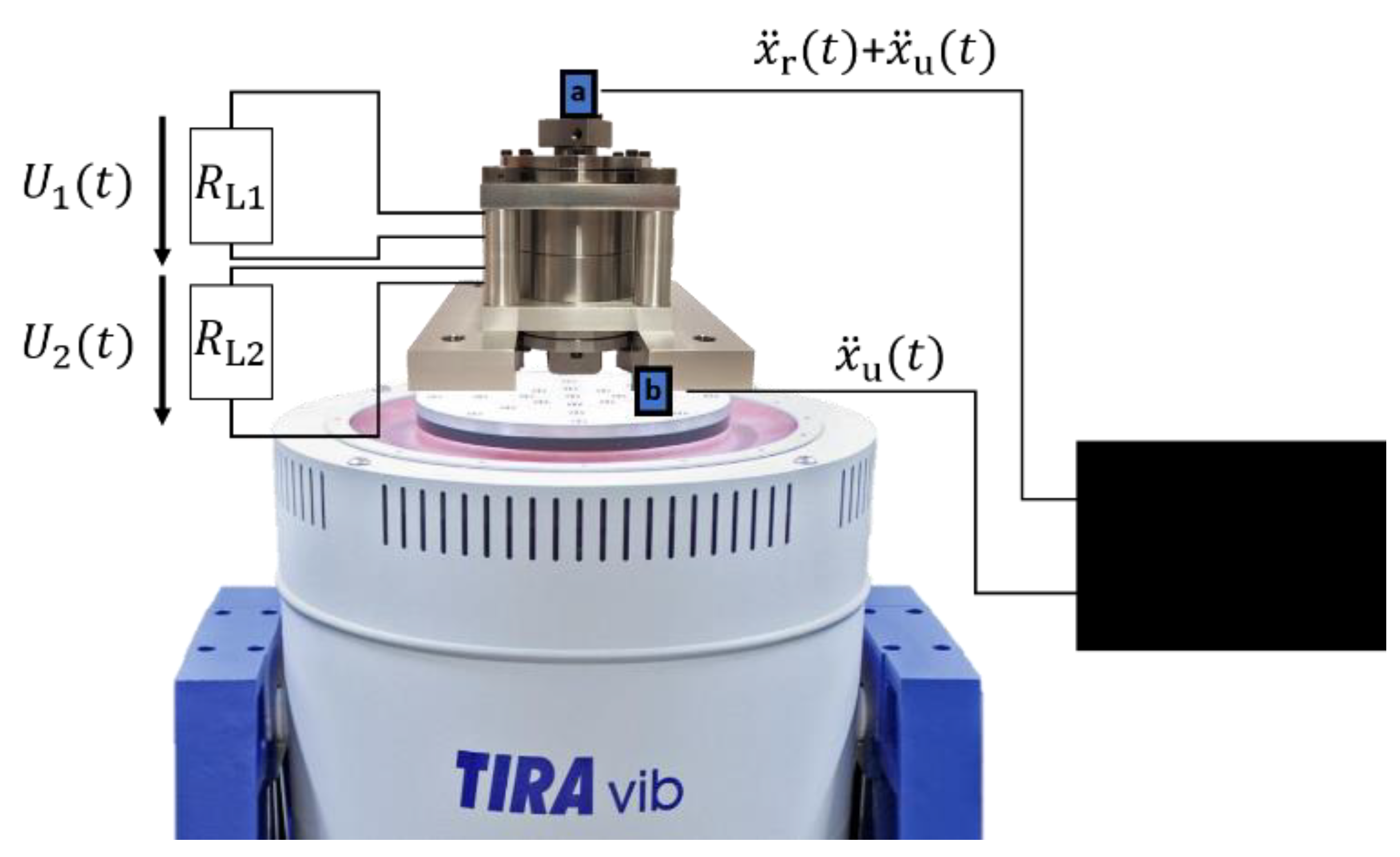
Figure 12.
Comparison between experimental and FEM results of the maximum relative amplitude for different mass–spring combinations. Solid line: experiment; dashed line: FEM.
Figure 12.
Comparison between experimental and FEM results of the maximum relative amplitude for different mass–spring combinations. Solid line: experiment; dashed line: FEM.
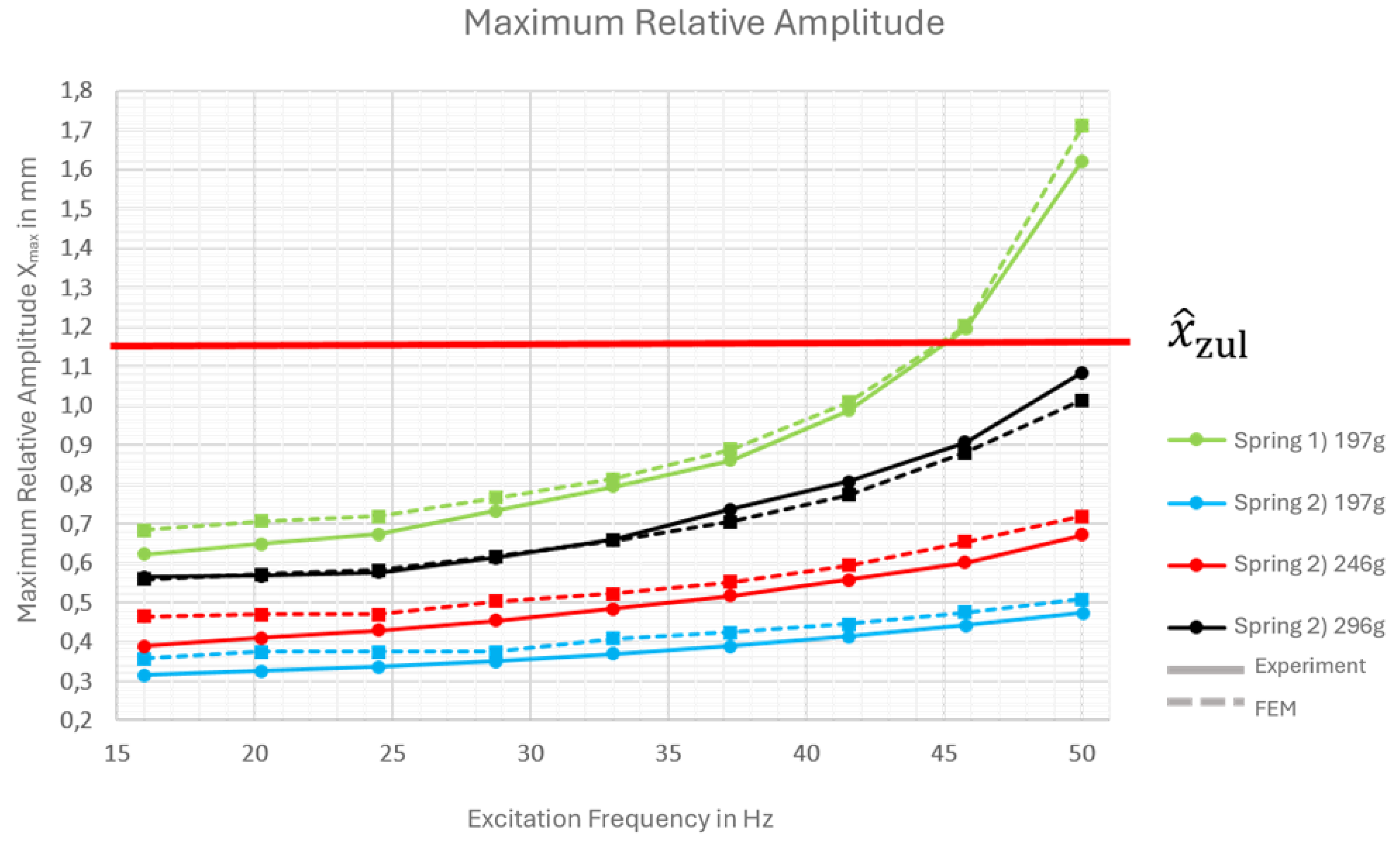
Figure 13.
Experimental setup showing the laboratory prototype, vibration exciter, acceleration sensors (a and b), load resistors (R_L1und R_L2), and the data acquisition board connected to the sensors.
Figure 13.
Experimental setup showing the laboratory prototype, vibration exciter, acceleration sensors (a and b), load resistors (R_L1und R_L2), and the data acquisition board connected to the sensors.
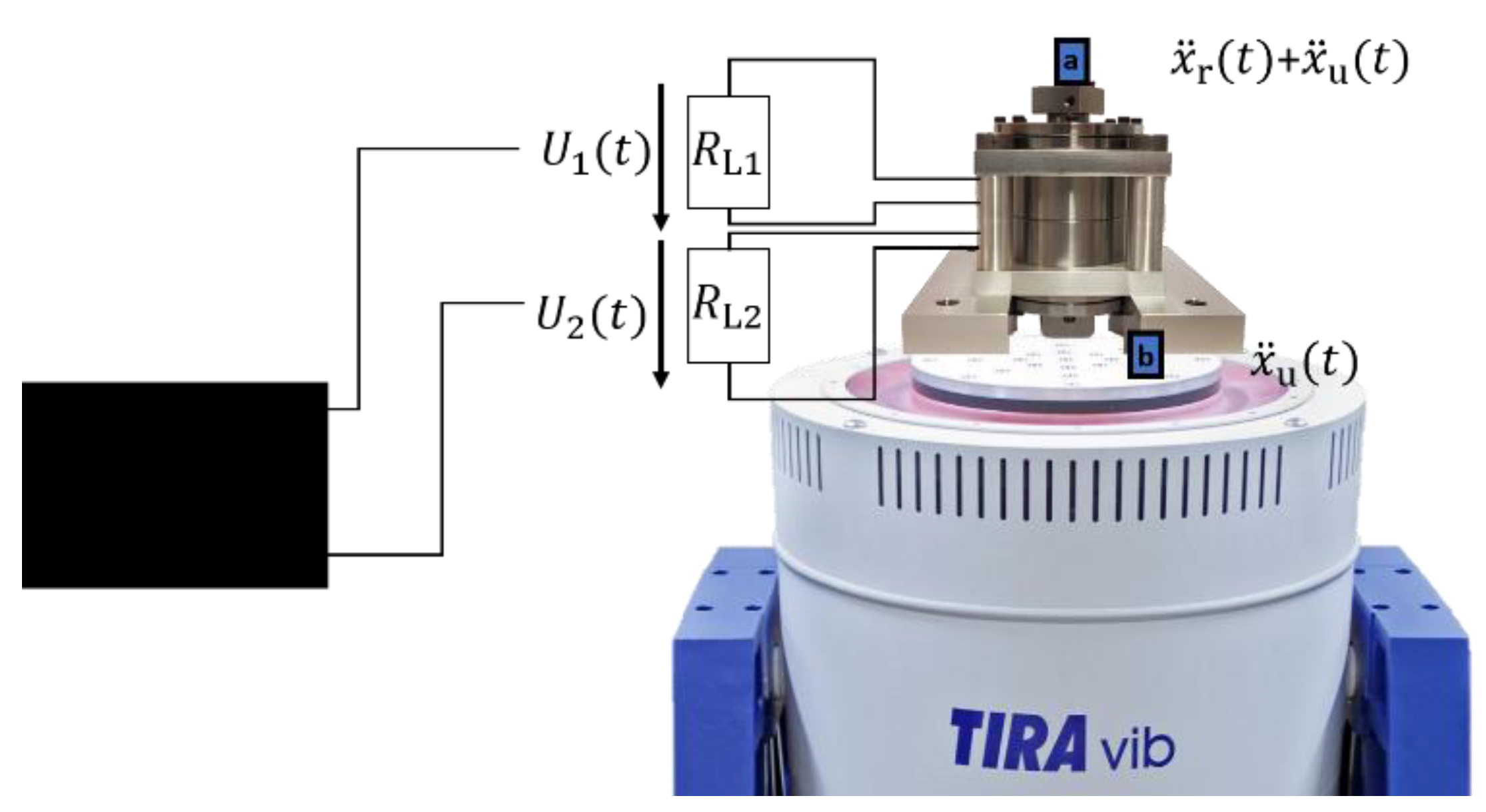
Figure 14.
Comparison between experimental and FEM results of the power output of the mass–spring combination (296 g and Spring 2) as a function of load resistance and excitation frequency at . Solid line: experiment; dashed line: FEM.
Figure 14.
Comparison between experimental and FEM results of the power output of the mass–spring combination (296 g and Spring 2) as a function of load resistance and excitation frequency at . Solid line: experiment; dashed line: FEM.
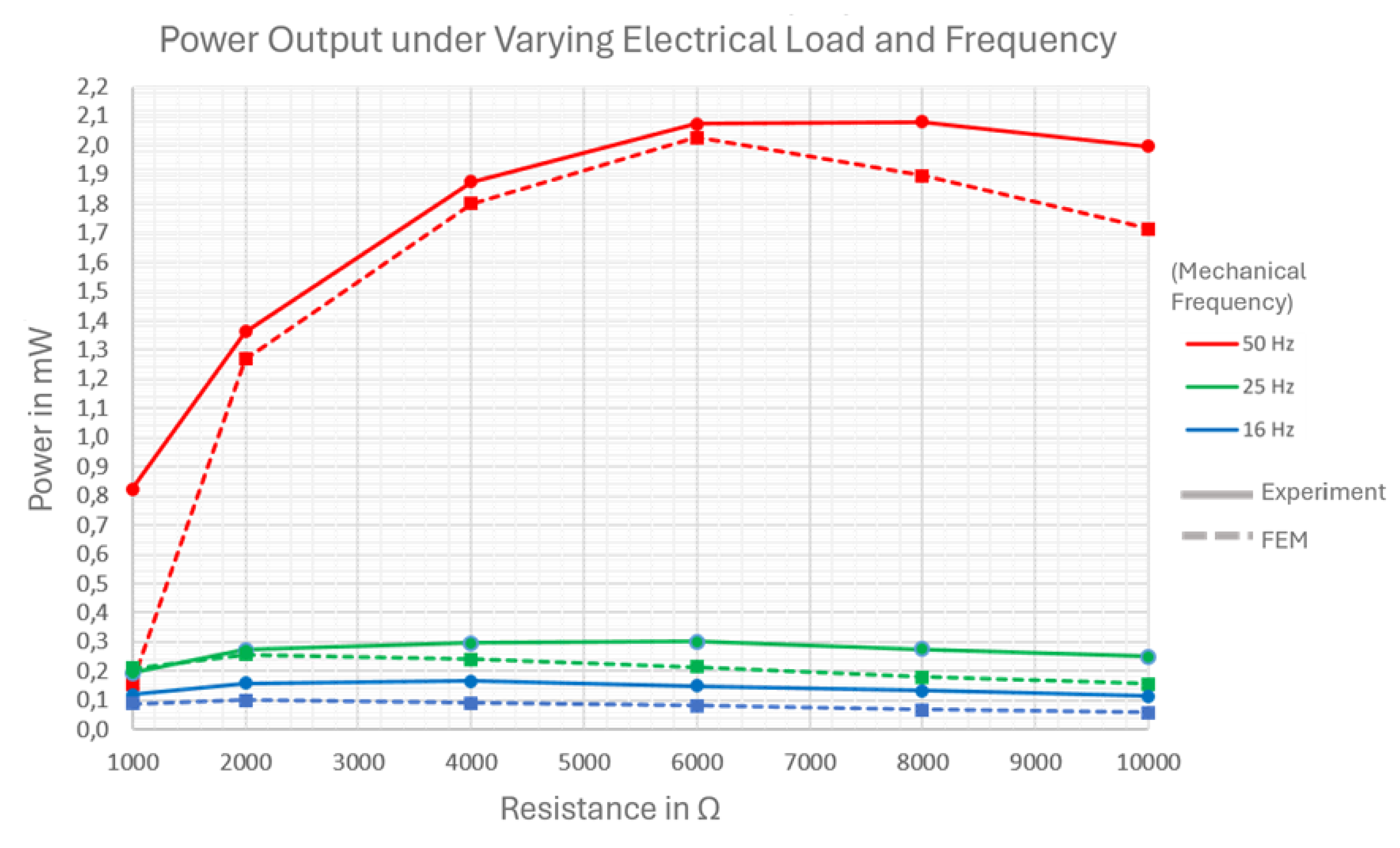
Table 1.
Parameters of NdFe35B35.
| Parameter | Description | Value |
|---|---|---|
| Remanence | ||
| Coercive field | ||
| Permeability |
Table 2.
Input parameters for excitation at (10g).
| Frequency (Hz) | Amplitude (mm) |
|---|---|
| 16 | 9,704 |
| 20.25 | 6,058 |
| 24.5 | 4,139 |
| 28.75 | 3,005 |
| 33 | 2,281 |
| 37.25 | 1,790 |
| 41.5 | 1,442 |
| 45.75 | 1,187 |
| 50 | 0,994 |
Disclaimer/Publisher’s Note: The statements, opinions and data contained in all publications are solely those of the individual author(s) and contributor(s) and not of MDPI and/or the editor(s). MDPI and/or the editor(s) disclaim responsibility for any injury to people or property resulting from any ideas, methods, instructions or products referred to in the content. |
© 2025 by the authors. Licensee MDPI, Basel, Switzerland. This article is an open access article distributed under the terms and conditions of the Creative Commons Attribution (CC BY) license (http://creativecommons.org/licenses/by/4.0/).
Copyright: This open access article is published under a Creative Commons CC BY 4.0 license, which permit the free download, distribution, and reuse, provided that the author and preprint are cited in any reuse.


