Submitted:
04 November 2025
Posted:
05 November 2025
You are already at the latest version
Abstract
Photoacoustic spectroscopy is a promising method for detecting dissolved acetylene (C2H2) in transformer oil, facilitating early fault diagnosis in power transformers. However, temperature variations significantly influence the resonance frequency of the photoacoustic cell, potentially reducing detection accuracy. This study investigates the temperature effects on the first-order longitudinal acoustic mode of a resonant photoacoustic cell using finite element simulations with thermo-viscous acoustics. Results show that as the temperature increases, the resonant frequency increases linearly and the sound pressure amplitude decreases, consistent with analytical models. To enhance system robustness, a perturbation-observation method is proposed, treating operating frequency as the independent variable and acoustic pressure as the dependent variable. Time-domain simulations validate its effectiveness in tracking resonance frequency shifts under varying temperatures, ensuring reliable detection. Future work should focus on improving frequency resolution, noise filtering, and adaptive step-size optimization for practical applications.
Keywords:
photoacoustic spectroscopy
; dissolved acetylene
; resonance frequency
; temperature effects
; perturbation-observation method
1. Introduction
Power transformers are critical components in electrical grids, and their reliable operation is essential for maintaining energy supply stability. Internal faults, such as partial discharges or overheating, can lead to the decomposition of insulating oil, generating dissolved gases like acetylene (C2H2), which serves as a key indicator of incipient failures [1,2,3]. Early detection of these gases enables preventive maintenance, reducing downtime and preventing catastrophic breakdowns [4]. Among various detection techniques, photoacoustic spectroscopy (PAS) has emerged as a promising method due to its high sensitivity, non-invasiveness, and ability to perform in-situ measurements [5,6,7,8]. In PAS, infrared laser light modulated at a specific frequency excites gas molecules, inducing periodic heating and subsequent acoustic waves that are detected in a resonant photoacoustic cell.
However, the performance of resonant PAS systems is highly susceptible to environmental variations, particularly temperature fluctuations. Temperature changes alter the speed of sound and dynamic viscosity of the gas medium within the photoacoustic cell, causing shifts in the resonance frequency and reductions in signal amplitude [9,10,11,12]. Such drifts can degrade detection accuracy, leading to false negatives or positives in acetylene monitoring, especially in field applications where transformers operate under varying ambient conditions [13,14,15,16]. Previous studies have quantified these effects through simulations and experiments, revealing linear frequency shifts of approximately 3 Hz per °C near room temperature [17]. Despite these insights, effective suppression strategies remain underexplored, limiting the robustness of PAS for real-time transformer health monitoring [18,19,20].
This paper addresses the temperature-induced challenges in PAS detection of dissolved acetylene in transformer oil by investigating the impact on photoacoustic cell resonance frequency and proposing a perturbation-observation method for suppression. Through finite element simulations using COMSOL, we model the frequency response under temperatures ranging from 0°C to 40°C, deriving analytical relationships for frequency shifts and amplitude variations. We then introduce a perturbation-observation algorithm that dynamically tracks the resonance frequency by applying small frequency perturbations and observing signal changes, ensuring optimal operation amid temperature variations. Simulation results in Simulink validate the method's efficacy in achieving rapid convergence to the resonance peak.
The remainder of this paper is organized as follows: Section 2 details the theoretical analysis and simulation of temperature effects on resonance frequency. Section 3 presents the perturbation-observation suppression method and its implementation. Section 4 experimental results. Finally, Section 5 conclusions.
2. Theoretical Analysis and Simulation of Temperature Effects on Resonance Frequency
2.1. Temperature Effects on Resonance Frequency
In resonant photoacoustic cells, operation requires modulating the incident infrared laser's photon frequency at a specific modulation frequency (corresponding to angular frequency ω). When using sinusoidal modulation (as shown in Figure 1a), the photon frequency varies over time as a central frequency superimposed with a sinusoidal component:
where γL is the half-width at half-maximum of the gas molecule absorption line, and m is the modulation depth.
Under this modulation, if the modulation center coincides with the center v0 of a gas molecule absorption line, the gas molecules in the photoacoustic cell will periodically absorb energy from the modulated laser, generating heat and exciting acoustic waves through thermo-acoustic coupling. The effective component of these acoustic waves has a frequency f = 2fm that is twice the modulation frequency fm, as illustrated in Figure 1b and Figure 1c. These acoustic waves interfere within the photoacoustic cell, eventually forming a stable standing wave distribution.
The photoacoustic cell itself has several acoustic vibration modes, each corresponding to a standing wave pattern and eigenfrequency fc. When the acoustic excitation source frequency fa approaches an eigenfrequency fc, the standing wave in the cell tends to distribute according to the corresponding pattern, resulting in a higher acoustic pressure amplitude Pm. Conversely, when the source frequency fa deviates from fc, the acoustic pressure amplitude Pm for that mode decreases.
When the background temperature T0 in the photoacoustic cell changes, the gas sound speed c0 and dynamic viscosity v change accordingly. The change in sound speed c0 causes a shift in the eigenfrequency fc, while the change in dynamic viscosity v affects the peak height of the response, causing the overall frequency response curve of the photoacoustic cell to shift, as shown in Figure 1d.
This subsection aims to use acoustic simulation, under a given geometric shape of the photoacoustic cell, to obtain the eigenfrequency fc of the first-order longitudinal acoustic vibration mode and the response peak of its frequency response curve Ac as a function of background temperature T0. Additionally, it seeks to obtain the frequency response curves of the photoacoustic cell at different background temperatures T0.
2.2. Simulation of Temperature Effects
Under the above geometric configuration, this report uses COMSOL's thermo-viscous acoustics module for simulation. A volumetric heat source H is used to equivalent the laser's effect, with the expression for H as follows:
where A2 is the second harmonic factor; c is the molar concentration of the gas to be measured; σ is the standard deviation parameter of the Gaussian beam.
This report sets the background temperature T at intervals of 5°C in the (0-40)°C range [i.e., (273.15-313.15) K] (including endpoints, totaling 9 groups). At each background temperature, frequency-domain simulations are performed with excitation frequencies in the (1520-1710) Hz range, sequentially obtaining the sound pressure distribution in the photoacoustic cell under sinusoidal steady state. The sound pressure at the axial center of the photoacoustic cell is used to measure the strength of the standing wave sound pressure. The response curve of the central sound pressure versus excitation frequency is plotted for each temperature, with the maximum point of the amplitude-frequency response curve at each temperature taken as the eigenfrequency for that temperature. The sound pressure data is normalized by the central sound pressure amplitude at the eigenfrequency under 20°C.
The simulation yields the curves of the photoacoustic cell eigenfrequency fc and normalized sound pressure amplitude as functions of background temperature T0, as shown in Figure 3. From the simulation results, it is evident that in the (0-40)°C temperature range, the eigenfrequency fc of the photoacoustic cell increases with rising background temperature T0, approximately in a linear relationship, with the eigenfrequency increasing by about 2.78 Hz per 1°C rise in background temperature. The sound pressure amplitude pn in the photoacoustic cell decreases with rising background temperature T0.
The simulation also yields the amplitude-frequency response curves of the photoacoustic cell at different temperatures, as shown in Figure 4. From the results, it can be seen that as temperature increases, the amplitude-frequency response curve of the photoacoustic cell shifts toward the lower right of the coordinate axis (i.e., higher frequency, lower amplitude); the eigenfrequency points fc and corresponding sound pressure amplitudes are approximately distributed along a straight line.
First, discuss the fc — T0 relationship. When a standing wave forms in the photoacoustic cell according to the first-order longitudinal acoustic vibration mode, the wavelength λ of the acoustic wave is approximately twice the length lr of the resonance tube:
Substituting this into the relationship among wavelength, frequency, and sound speed λf = c, the eigenfrequency fc is obtained:
where the sound speed , substituting into the above equation gives the relationship between fc and background temperature T0:
where γ is the specific heat ratio of the gas, generally taken as 1.4 for gases similar to air; R is the universal gas constant, with a value of 8.314 J/(K·mol); M is the average molar mass of the gas, generally taken as 29 g/mol for gases similar to air.
From (5), it is evident that the resonance frequency fc of the photoacoustic cell is proportional to the :
where the coefficient α is used to correct for non-ideal boundary conditions introduced by the buffer cavity and the disruption to the cylindrical geometric region caused by introducing the microphone cavity.
The value of coefficient k is calculated as 1715.08 Hz with the given parameters. Using the simulation value at 20°C to calculate the correction coefficient α, it is found to be 0.9440. The correction coefficient is close to 1, indicating that the approximation conditions underlying Equation (6) hold within the selected temperature range; the correction coefficient is slightly less than 1, consistent with the recognition that introducing the microphone cavity increases the resonance volume, slightly reducing the eigenfrequency compared to before introduction.
The eigenfrequencies for the remaining data points are calculated using the computed coefficients and compared with simulation results, with errors shown in Table 2.
From the error calculation results, it is evident that in the (0-40)°C temperature range, the change in the photoacoustic cell eigenfrequency fc with background temperature T0 approximately follows a linear relationship, and its slope can be obtained by measuring the eigenfrequency fc0 at a certain temperature point Tp and then dividing by 2TP. Near room temperature, a 1°C change in background temperature can cause a frequency shift of about 2.8 Hz.
Next, discuss the —T0 relationship. When the photoacoustic cell is excited acoustically at the eigenfrequency fc, if there is no loss in the gas within the cell, the sound pressure amplitude would theoretically be infinite. In other words, the presence of loss terms limits the sound signal amplitude at the resonance point in the photoacoustic cell. It is inferred that the background temperature T0 affects the sound pressure amplitude at the resonance point by influencing the loss terms. From previous studies, the loss in the photoacoustic cell depends on the viscous interaction between gases, and the strength of viscous loss is measured by the dynamic viscosity coefficient μ of the gas. The value of μ for the same gas is affected by its background temperature T0, with the relationship given by the Sutherland formula:
where Tp is a reference temperature, μp is the dynamic viscosity coefficient of the gas at that reference temperature; for air, when Tp is 288.15 K, μp is 1.7894×10⁻⁵ Pa·s; TB a constant, generally 110.4 K for air.
Intuitively, the larger the loss factor μ, the smaller the sound signal amplitude at the resonance point in the photoacoustic cell. Therefore, assume that and μ satisfy ∝1/μr relationship:
Using the least squares method to perform regression fitting on the simulation data according to the above equation, the parameters and r are obtained. The value of the proportional parameter is 192.3, with a 95% confidence interval of [189.7, 195.0]; the power parameter r is 2.086, with a 95% confidence interval of [2.081, 2.092]. The narrow 95% confidence intervals for both parameters, and the power coefficient r close to the integer 2, indicate that the adopted fitting model (8) has a high likelihood of conforming to physical reality.
The normalized amplitude of the sound signal in the photoacoustic cell at each temperature is calculated according to model (8) and its fitted coefficients, and compared with simulation values, with errors shown in Table 3.
From the error results, it is evident that for every 5°C rise in background temperature, the sound pressure at the resonance point attenuates by about 3%. The error between the simulation and formula value is close to 0, verifying that in the (0-40)°C temperature range, the sound pressure amplitude at the resonance point in the photoacoustic cell is approximately inversely proportional to the square of its dynamic viscosity μ.
3. Perturbation-Observation Suppression Method
3.1. Principle of the Perturbation-Observation Method
The perturbation-observation method is an approach for finding an approximate maximum point of a unimodal function. Its implementation is as follows: apply a perturbation amount to the independent variable, observe the change in the dependent variable, and check whether the signs of the perturbation and the change are consistent. If consistent, apply the perturbation amount to the independent variable again; otherwise, apply the perturbation amount in the reverse direction. Repeat the above process until the independent variable converges near the maximum point of the unimodal function. Since the frequency response curve of the photoacoustic cell is unimodal within a certain frequency range, the operating frequency f can be taken as the independent variable, the detected acoustic pressure amplitude Pm as the dependent variable, and a given step size for the operating frequency perturbation. Using the perturbation-observation method, the operating frequency can gradually converge near the resonant frequency of the photoacoustic cell. When the initial setting value of the operating frequency is on the left branch of the frequency response curve, the process of converging to the vicinity of the resonant frequency using the perturbation-observation method is shown in Figure 5.
During the operation of the photoacoustic cell, the acoustic pressure is measured by a microphone connected to the center of the photoacoustic cell and converted into a voltage signal. The latter is an AC voltage signal, which requires matching hardware circuits for detection and conversion into a DC signal that reflects its acoustic pressure amplitude. After each frequency perturbation is applied, the gas molecules in the cell need to undergo a certain relaxation time to reach a new steady-state acoustic pressure distribution; at the same time, the detection circuit also requires a certain response time. Therefore, applying the perturbation-observation method for resonance point tracking also requires a matching control timing sequence, as shown in Figure 6.
3.2. System Modeling and Equivalent Transfer Function
To verify the feasibility of using the perturbation-observation method for resonance point tracking, the physical processes involved in the photoacoustic cell from gas sound generation to microphone measurement of the acoustic signal are equivalent to the block diagram model shown in Figure 7, and time-domain simulation is performed using Simulink.
In the block diagram model, the photoacoustic cell is approximated as a link described by a frequency-domain transfer function, and this frequency-domain function varies with the temperature variable T. To describe the unimodal characteristics of the photoacoustic cell, a second-order bandpass transfer function is used for approximation:
where ω0 is the system's resonance point; A is the gain at the resonance point; ξ and Q are the system's damping ratio and quality factor, respectively, with the quantitative relationship Q = 1/(2ξ).
Previous studies based on acoustic finite element methods simulated the frequency response curves of the photoacoustic cell between 273.15 K and 313.15 K. This report uses the data at the resonance points and the 3 dB bandwidth to inversely calculate the parameters A, ω0, and Q in the equivalent second-order bandpass model of the photoacoustic cell. The parameters calculated according to the frequency response curves of the photoacoustic cell at 273.15 K, 293.15 K, and 313.15 K are shown in Table 4, and the system's amplitude-frequency response curves are shown in Figure 8.
3.3. Simulation Verification of the Control Method
To verify that the perturbation-observation method can track the resonance point of the photoacoustic cell under changing temperatures, a certain time-varying excitation is set for the temperature. This report adopts a three-stage temperature loading method, with the three stages of temperatures being T1, T2, and T3, each lasting for time ts. When the temperature set value changes, a negative exponential function with time constant τt is used for smooth transition. This loading method is shown in Figure 9.
4. Experimental Results
In the Simulink environment, the block diagram model shown in Figure 7 is built in Simulink, with the initial operating frequency f0 set to 1580 Hz and the frequency perturbation step size Δf set to 1 Hz. The three-stage temperatures are set to 273.15 K, 293.15 K, and 313.15 K, respectively, and the temperature transition time constant τt is taken as 2 s. The simulation results show the curves of the photoacoustic cell operating frequency f and acoustic signal P varying with time under the control of the perturbation-observation method, as shown in Figure 10.
From the results, it can be observed that the perturbation-observation method achieved the following operating path migration process, as depicted in Figure 11:
a. The photoacoustic cell starts from the zero-signal point at 0 and transitions to the operating point 1 corresponding to the initial set frequency at 273.15 K;
b. The operating frequency undergoes a negative perturbation, moving the operating point from 1 to the resonance point 2 at 273.15 K, while the operating frequency oscillates around the resonance frequency;
c. The temperature changes to 293.15 K, causing the operating point to drop from 2 to point 3 on the amplitude-frequency curve at 293.15 K;
d. The operating frequency undergoes a positive perturbation, moving the operating point from 3 to the resonance point 4 at this temperature, and oscillating around it;
e. The temperature changes to 313.15 K, causing the operating point to drop from 4 to point 5 on the amplitude-frequency curve at 313.15 K;
f. The operating frequency undergoes a positive perturbation, moving the operating point from 5 to the resonance point 6 at this temperature, and oscillating around it.
5. Conclusions
The aforementioned results demonstrate that the perturbation-observation method enables automatic tracking of the photoacoustic cell's resonance point in response to temperature variations. However, for this method to be practically implemented, several key challenges must be addressed:
(1) The frequency resolution of the signal generator controlling laser wavelength modulation imposes a lower limit on the frequency perturbation step length;
(2) The voltage signal output from the microphone, which measures the acoustic signal, may be overwhelmed by noise, necessitating appropriate filtering of the electrical signal if such interference occurs;
(3) When the initial frequency deviates significantly from the resonance frequency under operating temperature conditions, a larger frequency perturbation step is desirable to expedite the convergence of the working frequency toward the resonance frequency; conversely, once the working frequency approaches the resonance frequency, a smaller step is preferable to minimize signal fluctuations. Resolving this inherent trade-off requires optimization of the step values based on specific operational scenarios;
(4) The implementation of perturbation-observation control encompasses multiple physical relaxation processes and transitional phases within the measurement system's circuitry, demanding meticulous tuning of the controller's timing sequence.
Author Contributions
Conceptualization, H.N.; methodology, J.W.; software, X.W.; validation, J.S.; formal analysis, Z.W.; investigation, L.H.; data curation, H.N.; writing—original draft preparation, H.N.; writing—review and editing, Z.W. and J.W.; supervision, Q.Z.; All authors have read and agreed to the published version of the manuscript.
Funding
This research was funded by State Grid Corporation of China Science and Technology Project, grant number 520940240010.
Data Availability Statement
Data are contained within the article.
Conflicts of Interest
The authors declare no conflicts of interest. Authors Heli Ni, Xinye Wu and Lin He were employed by State Grid Shanghai Electric Power Research Institute. The remaining authors declare that the research was conducted in the absence of any commercial or financial relationships that could be construed as a potential conflict of interest.
References
- He Z; Zhao L; Zhao Y; Sun X; Jiang T; Bao L. Dissolved gases generated of partial discharges and electrical breakdown in oil-paper insulation under AC-DC combined voltages. 2012 International Conference on High Voltage Engineering and Application. Shanghai, China, 2012, 314-371. [CrossRef]
- Luo B; Wang J; Dai D; Lei J; Li L; Wang T. Partial discharge simulation of air gap defects in oil-paper insulation paperboard of converter transformer under different ratios of AC–DC combined voltage. Energies, 2021, 14, 6995. [Google Scholar] [CrossRef]
- Chen T; Ma F; Zhao Y; Zhao Y; Wan L; Li K; Zhang G. Portable ppb-level acetylene photoacoustic sensor for transformer on-field measurement. Optik, 2021, 243, 167440. [Google Scholar] [CrossRef]
- Ward, S.A. Evaluating transformer condition using DGA oil analysis. 2003 Annual Report Conference on Electrical Insulation and Dielectric Phenomena, Albuquerque, NM, USA, 2003, 463-468. [CrossRef]
- Bakar N A; Abu-Siada A. A new method to detect dissolved gases in transformer oil using NIR-IR spectroscopy. IEEE Trans. Dielectr. Electr. Insul., 2017, 24, 409–419. [Google Scholar] [CrossRef]
- Rosencwaig, A. Photoacoustics and photoacoustic spectroscopy. Wiley, New York, 1981. [CrossRef]
- Schilt S; Thévenaz L. Wavelength modulation photoacoustic spectroscopy: Theoretical description and experimental results. Infrared Phys. Technol., 2006, 48, 154–162. [Google Scholar] [CrossRef]
- Mao Zhixin; Wen Jinyu. Detection of dissolved gas in oil–insulated electrical apparatus by photoacoustic spectroscopy. IEEE Electr. Insul. Mag., 2015, 31, 7–14. [Google Scholar] [CrossRef]
- Wei C; Ju T; Lin C; Zhang C; Fan M; Zhou Q. Detection of SF6 decomposition components under partial discharge by photoacoustic spectrometry and its temperature characteristic. IEEE Trans. Instrum. Meas., 2016, 65, 1343–1351. [Google Scholar] [CrossRef]
- General Administration of Quality Supervision, Inspection and Quarantine of the People's Republic of China. GB/T 7252-2001, Guidelines for Analysis and Judgment of Gases Dissolved in Transformer Oil. Standards Press: Beijing, China, 2002.
- Wei Q; Chen W; Xiong Y. The research on simultaneous detection of dissolved gases in transformer oil using Raman spectroscopy. 2015 IEEE Electrical Insulation Conference (EIC), Seattle, WA, USA, 2015, 154-157. [CrossRef]
- Simon P; Moulin B; Buixaderas E; Raimboux N; Herault E; Chazallon B; Cattey H; Magneron N; Oswalt J; Hocrelle D. High temperatures and Raman scattering through pulsed spectroscopy and CCD detection. J. Raman Spectrosc., 2003, 34, 497–504. [Google Scholar] [CrossRef]
- Filippov V P; Salomasov V A. Mössbauer spectroscopy in determining the gas molecular state. Hyperfine Interact, 2016, 237, 35. [Google Scholar] [CrossRef]
- Koskinen V; Fonsen J; Kauppinen J; Kauppinen I. Extremely sensitive trace gas analysis with modern photoacoustic spectroscopy. Vib. Spectrosc., 2006, 42, 239–242. [Google Scholar] [CrossRef]
- Liu X; Cheng S; Liu H; Sha H; Zhang D; Ning H. A survey on gas sensing technology. Sensors 2012, 12, 9635–9665. [Google Scholar] [CrossRef] [PubMed]
- Kästle R; Sigrist M W. Temperature-dependent photoacoustic spectroscopy with a Helmholtz resonator. Appl. Phys. B, 1996, 63, 389–397. [Google Scholar] [CrossRef]
- Borozdin P; Erushin E; Kozmin A; Bednyakova A; Miroshnichenko I; Kostyukova N; Boyko A; Redyuk A. Temperature-Based Long-Term Stabilization of Photoacoustic Gas Sensors Using Machine Learning. Sensors 2024, 24, 7518. [CrossRef] [PubMed]
- Niu M; Liu Q; Liu K; Yuan Y; Gao X. Temperature-dependent photoacoustic spectroscopy with a T shaped photoacoustic cell at low temperature. Opt. Commun., 2013, 287, 180–186. [Google Scholar] [CrossRef]
- Angeli G Z; Bozóki Z; Miklós A; Lörincz A; Thöny A; Sigrist M W. Design and characterization of a windowless resonant photoacoustic chamber equipped with resonance locking circuitry. Rev. Sci. Instrum., 1991, 62, 810–813. [Google Scholar] [CrossRef]
- Li Yangliu. On-line Analysis Technology of Dissolved Gases in Insulating Oil Based on Membrane Separation and Photoacoustic Spectroscopy. Harbin Institute of Technology, PhD dissertation, Harbin, China, 2011.
Figure 1.
Various physical processes in the photoacoustic cell. (a) Schematic of laser wavelength modulation; (b) Excited heating of gas molecules; (c) Acoustic pressure waveform from thermo-acoustic effect; (d) Frequency shift caused by temperature change.
Figure 1.
Various physical processes in the photoacoustic cell. (a) Schematic of laser wavelength modulation; (b) Excited heating of gas molecules; (c) Acoustic pressure waveform from thermo-acoustic effect; (d) Frequency shift caused by temperature change.
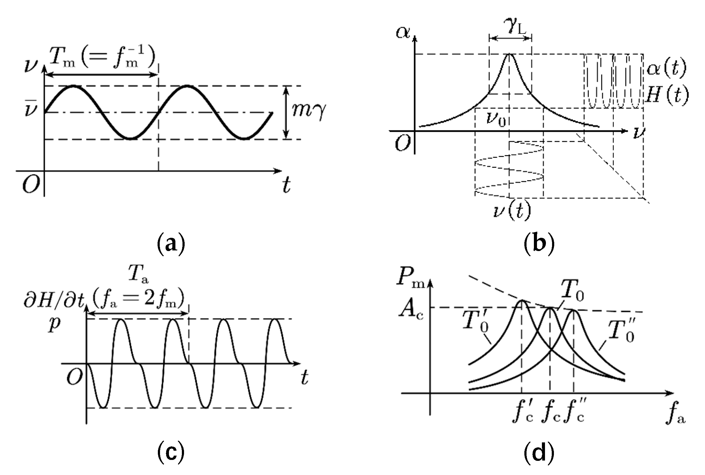
Figure 2.
Schematic of microphone cavity geometry. (1—Buffer cavity; 2—Resonance tube; 3—Connection hole; 4—Microphone cavity; 5—Microphone).
Figure 2.
Schematic of microphone cavity geometry. (1—Buffer cavity; 2—Resonance tube; 3—Connection hole; 4—Microphone cavity; 5—Microphone).
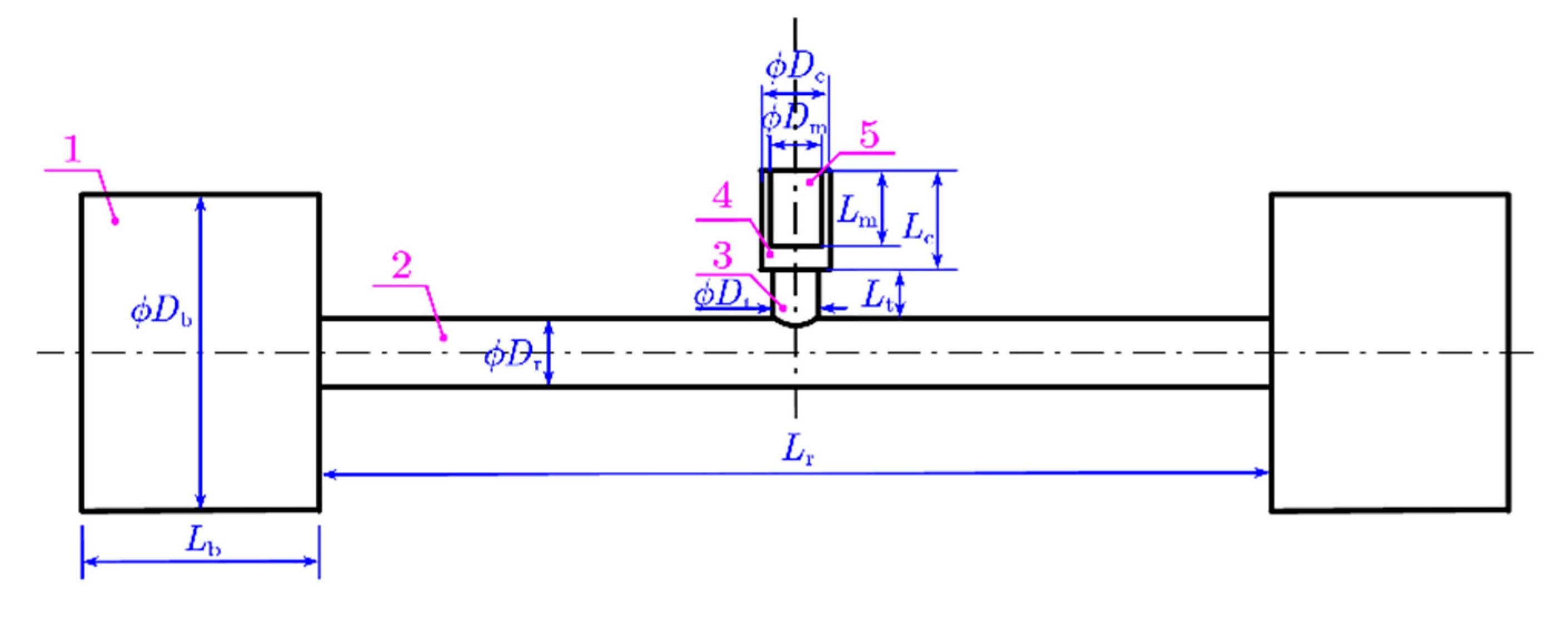
Figure 3.
Eigenfrequency/sound pressure amplitude - background temperature curves.
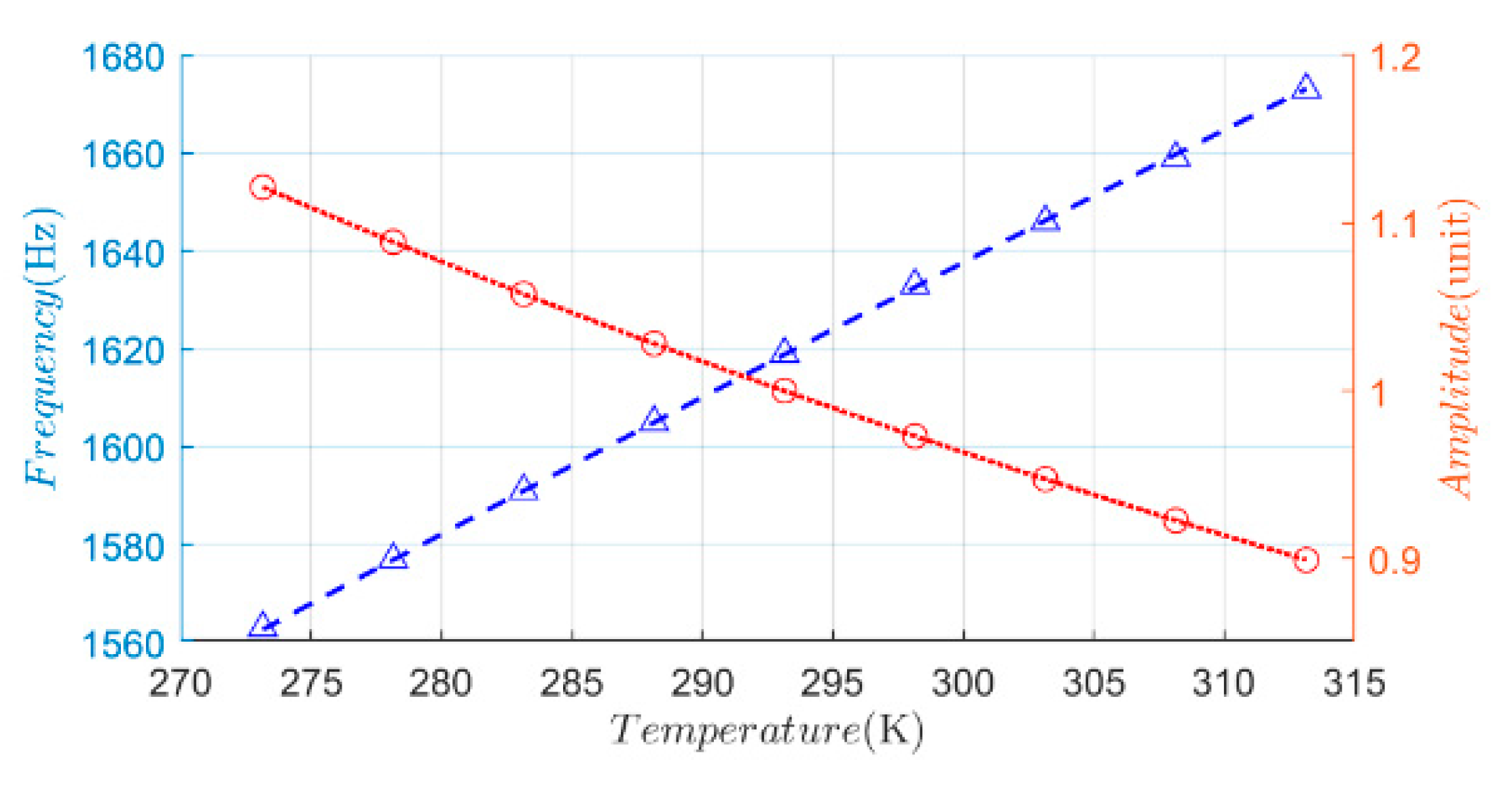
Figure 4.
Amplitude-frequency response curves of the photoacoustic cell.
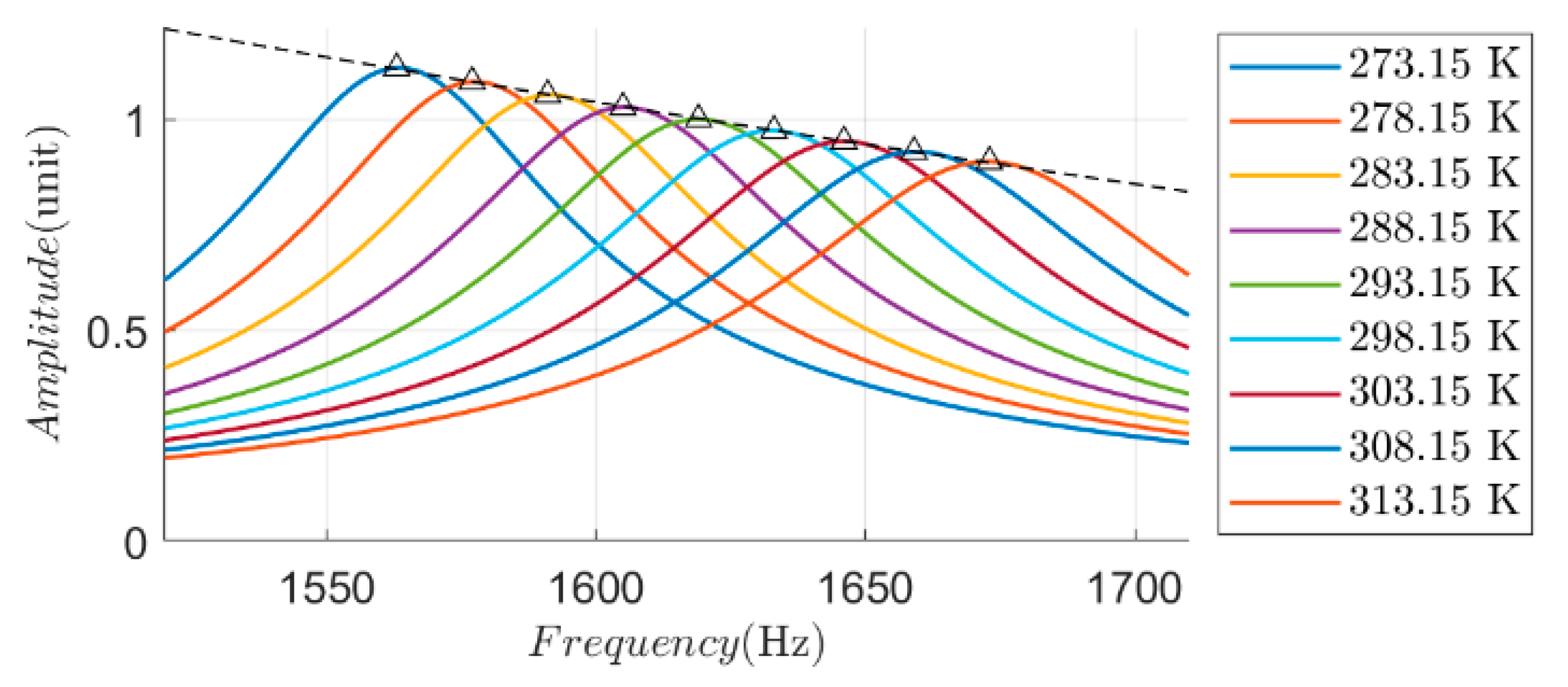
Figure 5.
Schematic diagram of resonance point tracking using the perturbation-observation method. (In the figure, Δf represents the frequency perturbation step size, and f(k) represents the operating frequency after the k-th perturbation is applied.).
Figure 5.
Schematic diagram of resonance point tracking using the perturbation-observation method. (In the figure, Δf represents the frequency perturbation step size, and f(k) represents the operating frequency after the k-th perturbation is applied.).
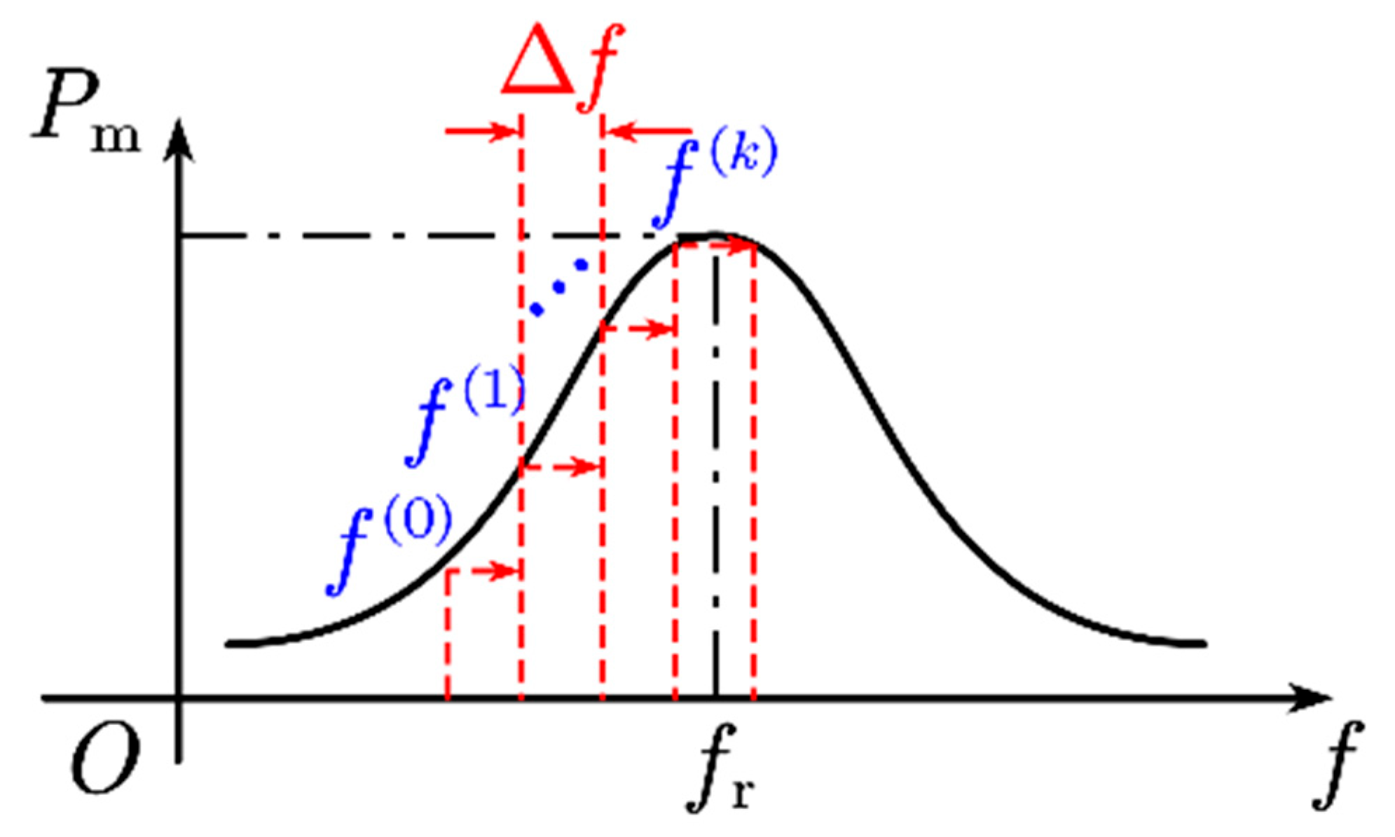
Figure 6.
Program block diagram for resonance point tracking using the perturbation-observation method. (In the figure, D is the direction factor, indicating the direction of the applied frequency perturbation.).
Figure 6.
Program block diagram for resonance point tracking using the perturbation-observation method. (In the figure, D is the direction factor, indicating the direction of the applied frequency perturbation.).
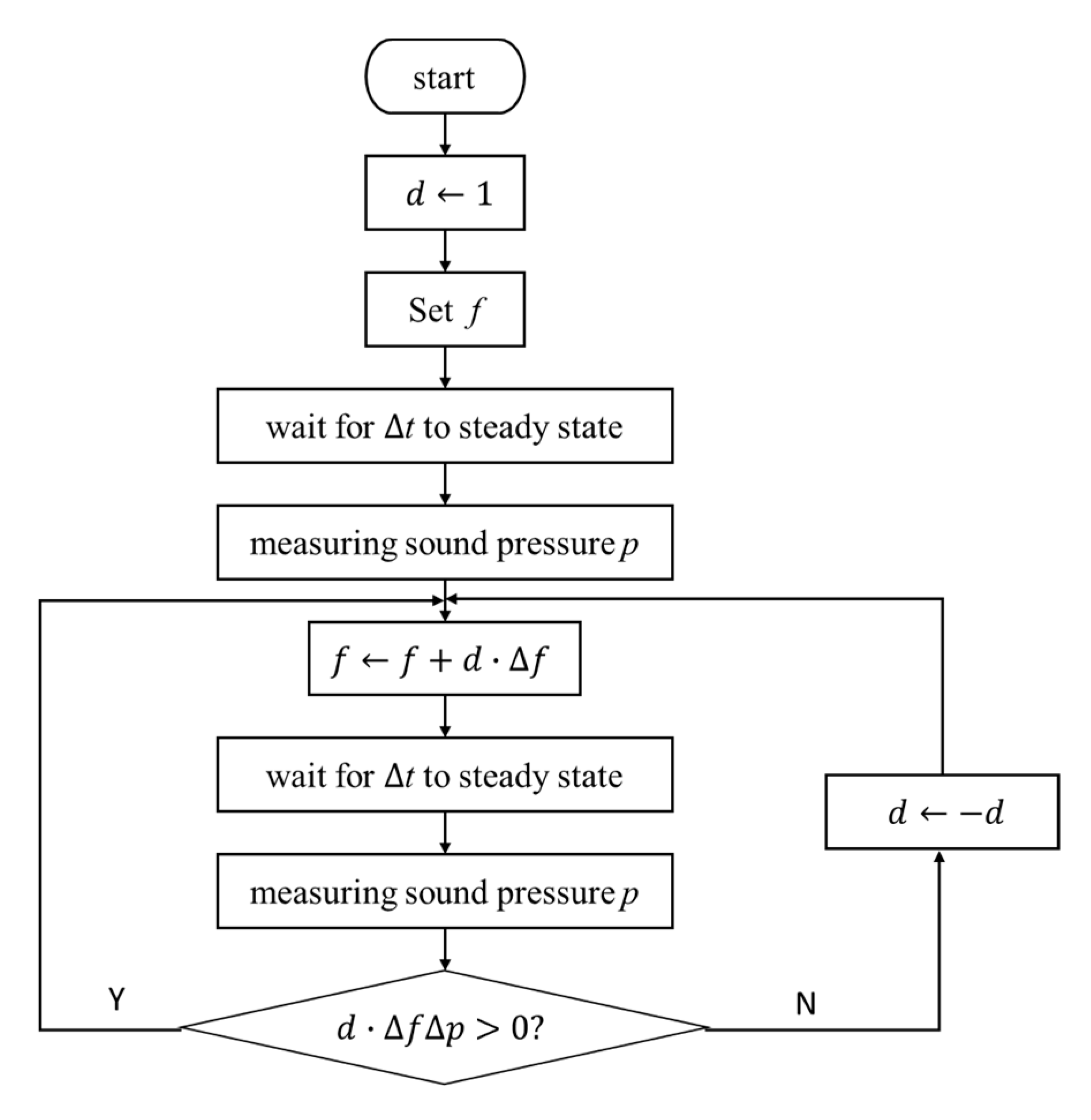
Figure 7.
Block diagram model of the photoacoustic cell system. (In the figure, f0 represents the initial operating frequency; Δf is the frequency perturbation step size; System represents the equivalent frequency-domain model of the photoacoustic cell; Microphone represents the acoustic-to-electric conversion link of the microphone.).
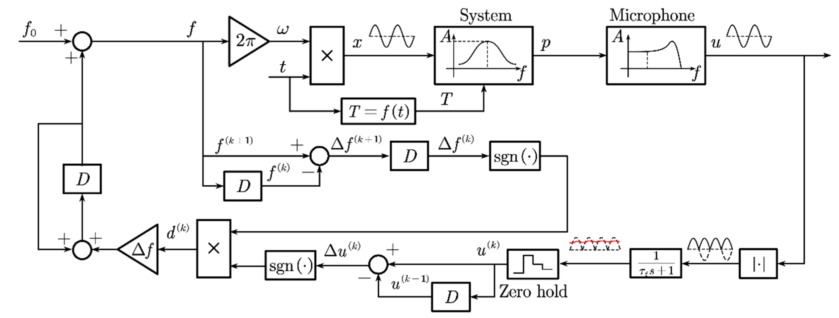
Figure 8.
Amplitude-frequency response curves of the approximate second-order bandpass model for the photoacoustic cell.
Figure 8.
Amplitude-frequency response curves of the approximate second-order bandpass model for the photoacoustic cell.
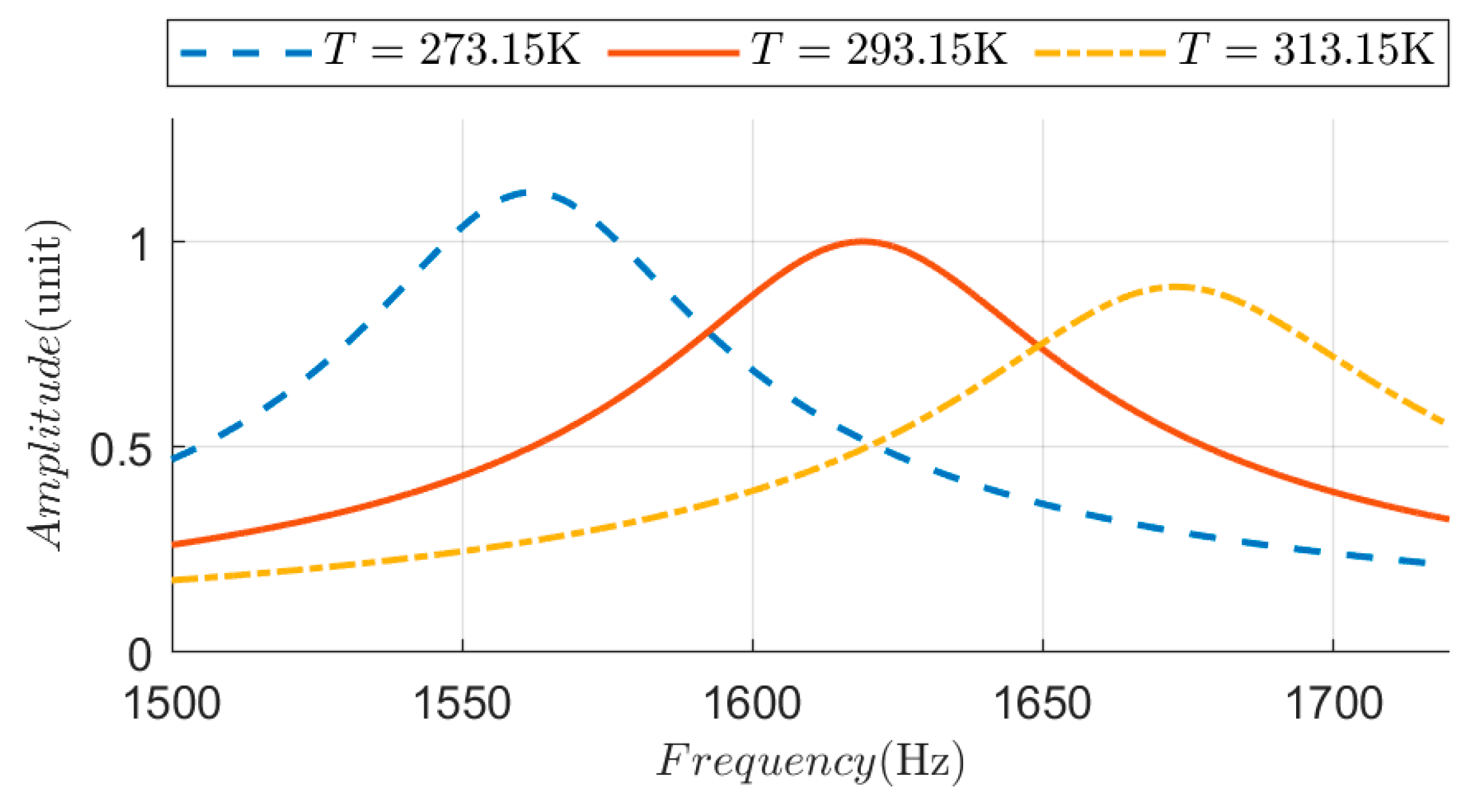
Figure 9.
Temperature loading method.

Figure 10.
Verification results of the perturbation-observation control strategy.
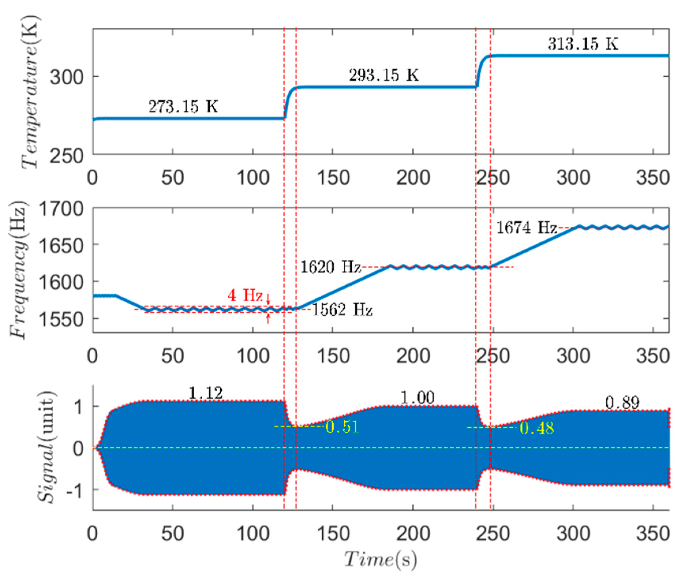
Figure 11.
Migration of the photoacoustic cell operating path.
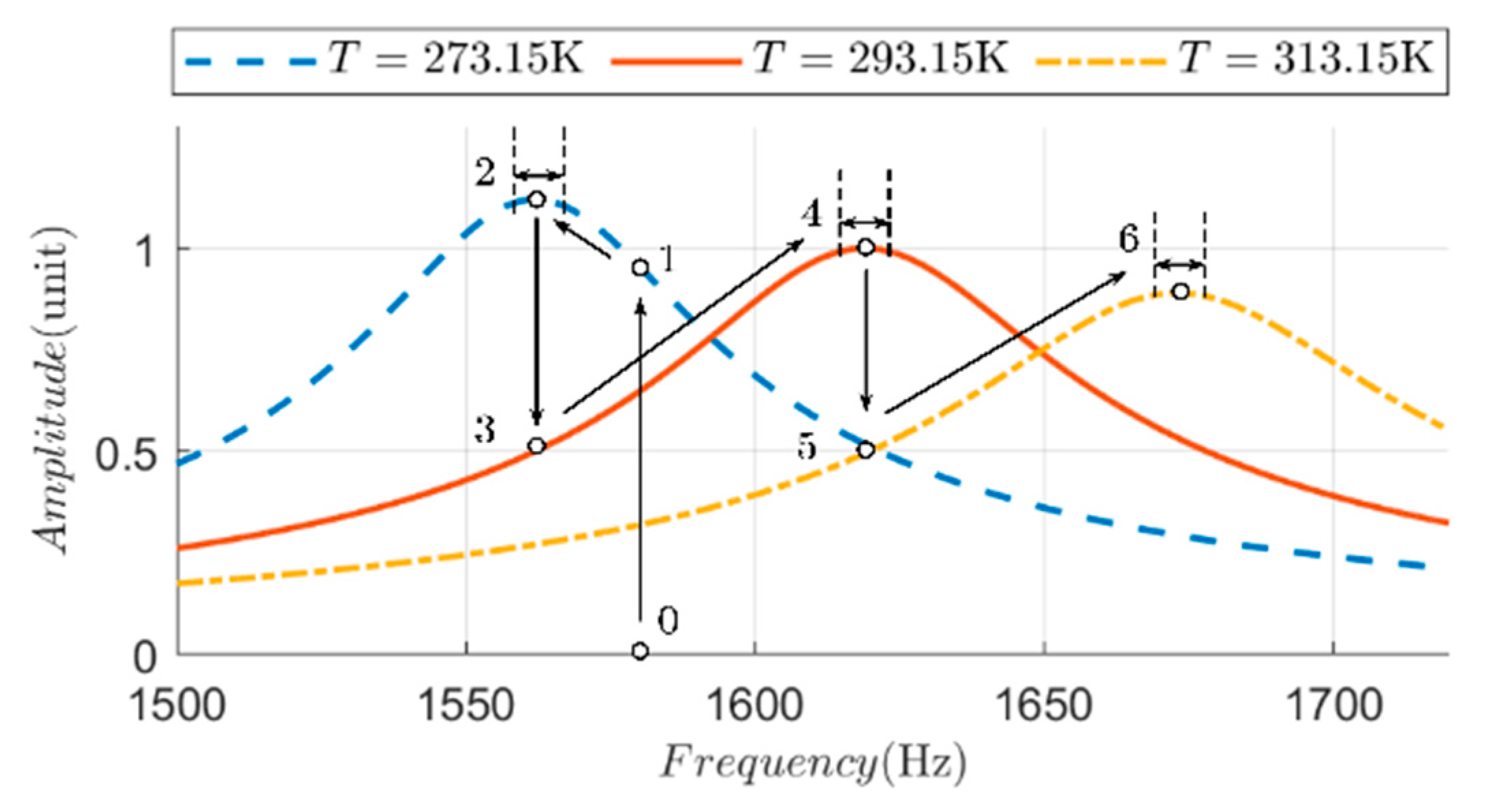

Table 1.
Geometric parameters of the photoacoustic cell.
| Geometric Parameter | Value | Geometric Parameter | Value |
|---|---|---|---|
| Db | 20 mm | Lb | 50 mm |
| Dr | 3 mm | Lr | 100 mm |
| Dt | 1 mm | Lt | 1 mm |
| Dc | 3 mm | Lc | 4.3 mm |
| Dm | 2.8 mm | Lm | 3.3 mm |
Table 2.
Errors in eigenfrequency formula.
| Temperature/°C | 0 | 5 | 10 | 15 | 20 | 25 | 30 | 35 | 40 |
|---|---|---|---|---|---|---|---|---|---|
| Simulation value/Hz | 1562.4 | 1576.5 | 1590.6 | 1604.9 | 1619.1 | 1632.7 | 1646.1 | 1659.0 | 1673.2 |
| Formula value/Hz | 1563.9 | 1577.7 | 1591.5 | 1605.3 | 1919.1 | 1632.9 | 1646.7 | 1660.5 | 1674.3 |
| Error value/Hz | 1.5 | 1.2 | 0.9 | 0.4 | — | 0.2 | 0.6 | 1.5 | 1.1 |
| 2.78 | 2.76 | ||||||||
Table 3.
Errors in sound pressure amplitude formula.
| Temperature/°C | 0 | 5 | 10 | 15 | 20 | 25 | 30 | 35 | 40 |
|---|---|---|---|---|---|---|---|---|---|
| Simulation value/unit | 1.1213 | 1.0887 | 1.0577 | 1.0281 | 1.0000 | 0.9729 | 0.9473 | 0.9227 | 0.8991 |
| Formula value/ unit | 1.1229 | 1.0900 | 1.0587 | 1.0291 | 1.0001 | 0.9739 | 0.9483 | 0.9239 | 0.9005 |
| Error value/unit | 0.0016 | 0.0013 | 0.0010 | 0.0010 | 0.0001 | 0.0010 | 0.0010 | 0.0012 | 0.0014 |
Table 4.
Calculated parameters for the approximate second-order bandpass model of the photoacoustic cell.
Table 4.
Calculated parameters for the approximate second-order bandpass model of the photoacoustic cell.
| T(K) | 273.15 | 293.15 | 313.15 |
| f0(Hz) | 1562 | 1619 | 1673 |
| A(1) | 1.12 | 1.00 | 0.89 |
| Q(1) | 26.74 | 24.12 | 22.74 |
Disclaimer/Publisher’s Note: The statements, opinions and data contained in all publications are solely those of the individual author(s) and contributor(s) and not of MDPI and/or the editor(s). MDPI and/or the editor(s) disclaim responsibility for any injury to people or property resulting from any ideas, methods, instructions or products referred to in the content. |
© 2025 by the authors. Licensee MDPI, Basel, Switzerland. This article is an open access article distributed under the terms and conditions of the Creative Commons Attribution (CC BY) license (http://creativecommons.org/licenses/by/4.0/).
Copyright: This open access article is published under a Creative Commons CC BY 4.0 license, which permit the free download, distribution, and reuse, provided that the author and preprint are cited in any reuse.


