
Submitted:
03 November 2025
Posted:
04 November 2025
You are already at the latest version
Abstract
Tailings reservoir is an important part of the mine. The monitoring and assessment of the stability of their key structures have always been the focus of research by many scholars. In this experiment, Interferometric Synthetic Aperture Radar (InSAR) and the Global Navigation Satellite System (GNSS) were employed to obtain 30 sets of longitudinal deformation data of 6 feature monitoring points on the surface of a tailings reservoir in Anhui Province. Considering the complementarity of InSAR and GNSS in surface monitoring, it is proposed to calculate the optimal initial parameters Q and R of Kalman filter by using Particle Swarm Optimization ( PSO ), so as to construct the optimal PSO-Kalman data assimilation model to achieve bidirectional data assimilation between InSAR and GNSS data, improve the accuracy of InSAR data, and comprehensively analyze the stability of key dams. After that, the Long Short Term Memory (LSTM) recurrent neural network is utilized to conduct time series predictions on the assimilated data and the buried depth data of the saturation line of the monitoring points of the mine dam during the same period. The experimental results show that using PSO-Kalman filter for data assimilation, compared with the original InSAR data, the overall mean absolute error ( MAE ) is reduced by 52.7 %, and the overall root mean square error ( RMSE ) is reduced by 53.6 %. By using LSTM to predict the time series data, the RMSE of the key dam deformation data test output set is less than 2.5mm, and the RMSE of the saturation line buried depth test output set is less than 1.5mm. Finally, the existing data is used to train the dam stability evaluation model. Under the condition that the correct rate of the evaluation model is 88.89 % and the AUC value of the model stability is 0.88889, the LSTM prediction data and the stability evaluation model are used to analyze the future stability of the key structure. This paper innovatively proposes to jointly evaluate the stability of the key dam structure by combining the deformation data and the saturation line height data. It also presents the first relatively complete integrated research method of ' monitoring-prediction-evaluation ' for the key dam body of the tailings reservoirs. The experimental results show that this method can provide reliable data and technical support for the monitoring, stability analysis and evaluation of the key dam body of tailings reservoirs.
Keywords:
PSO-Kalman filter
; InSAR
; data assimilation
; PCA-RF
; stability evaluation of tailings reservoirs
1. Introduction
The tailings reservoirs are places for storing and managing tailings or other industrial waste discharged after ore separation and processing in each mine [1]. It is an artificial debris flow with a risk of dam collapse. Once the key dam body collapses, it will cause extremely serious damage to the environment and residential facilities downstream of the tailings pond. According to statistics, the probability of tailings dam break is relatively high, with an average of two to five large tailings ponds worldwide breaking each year [2]. There are more than 8000 tailings reservoirs in China, ranking first in the world, and most of them are located in the valleys along the rivers in mountainous areas, presenting a typical distribution characteristic of the river basin. Once accidents such as leakage and dam break occur, they are easy to flow into low-lying valleys and rivers, causing secondary environmental pollution along the river. Therefore, the monitoring of the surface deformation of the tailings dam body and the stability evaluation and analysis of the tailings pond are indispensable in China.
In recent years, many scholars have carried out a lot of experimental research on the safety of tailings dam. Yang Chunhe [3] conducted a systematic study on the disaster mechanism and prevention and control methods of the key dam body of tailings ponds. His team discussed the stability of the key dam body through theoretical analysis and numerical simulation. To obtain sufficient data on the stability of the key dam body, a monitoring system that integrates different methods is needed. The representative achievements in the monitoring and analysis of the stability of tailings dam bodies are as follows: Risk monitoring of tailings dam bodies, Liu Pei et al. [4] used the deep semantic segmentation method to process GF1 satellite images, and comprehensively analyzed the stability of the tailings dam body and the hazards caused by dam failure. Yan Shiyong et al. [5] conducted wide-area monitoring of the stability of tailings dam groups by using the improved maximum likelihood estimation and the DS-InSAR technology with joint distributed targets, achieving certain results. Wang Guangjin et al.[6] introduced the structural importance coefficient using the BowTie model to analyze the influence of the water table height on the tailings dam body. Their research results can provide reliable technical support for the design and stability evaluation of the dam body. In addition to on-site monitoring, Zhao et al. conducted physical experiments, using digital image technology to simulate the changes of saturation line and dam deformation under rainfall conditions in tailings reservoir. The study showed that the height of the saturation line has a significant impact on the stability of the dam body, and is of great importance for the monitoring of key dam bodies of the tailings pond. Meanwhile, a large number of deformation data were obtained by monitoring. Hu Jun et al. [7] used the cuckoo algorithm to optimize the SVM model, which solved the problem of excessively long fitting accuracy and poor robustness of the SVM model. The final experiment showed that the fitting time of this model was reduced and the robustness was improved. In view of the current research results, many scholars have mainly conducted studies on the key dam body monitoring and stability of tailings ponds from the perspectives of single monitoring techniques, data analysis, and numerical simulation. There are few ways to assimilate data using different monitoring technologies and models. This paper proposes to adopt the collaborative monitoring of InSAR and GNSS technologies for data assimilation and prediction.
Interferometric Synthetic Aperture Radar,InSAR,a new type of microwave remote sensing technology for the Earth developed in recent years. It can meet the requirements of high-precision, large-scale, and round-the-clock monitoring at a low cost. However, due to its own technical limitations, it is susceptible to atmospheric delay errors, temporal-spatial decoherence noise, and changes in the ground environment, etc. [8,9], resulting in the resolution in the time domain not reaching very high requirements and including certain gross errors in the measurement results. It is suitable for obtaining displacement and deformation information of the surface of tailings dam bodies with large areas. The development of Global Navigation Satellite System(GNSS) has provided high-precision continuous monitoring information for surface deformation monitoring. Research institutions can obtain high-time-resolution and high-precision deformation information by setting up GNSS continuous monitoring devices at ground points in the monitoring area. However, since GNSS is a monitoring technology based on a single base station, its spatial resolution and monitoring cost are limited by the number and networking form of GNSS devices. It is quite difficult to realize monitoring in large areas like tailings dams [10]. GNSS can continuously and rapidly provide punctiform time-series deformation information with millimeter-level accuracy. However, due to the high cost of its monitoring equipment, it is difficult to set up a large number of monitoring points over a wide area, making it hard to obtain high spatial resolution dam deformation data and failing to meet the requirements of large-scale monitoring fields. In contrast, InSAR can acquire deformation fields over a wide area, but it is susceptible to factors such as long time spans, large deformation amplitudes, and atmospheric interference, resulting in the inability to obtain high time-series dam deformation data and having the defect of insufficient time resolution. The Long Short Term Memory ( LSTM ) was used to predict the fused deformation data and the height of the saturation line of the tailings dam at the same period. Based on the predicted settlement data and the height of the saturation line, a Principal Component Analysis (PCA) - Random Forest (RF) evaluation model was constructed. This paper innovatively and initialtively proposes joint evaluation of the time-series stability of the tailings dam by using the predicted settlement data and the height of the saturation line, providing reliable technical support for the long-term safe operation of the critical dam body.
2. Materials and Methods
2.1. Study Area and Data Acquisition
The research area of this paper is the Houjiachong tailings reservoir of a mining company in Anhui Province. The dam not only ensures the safety of the tailings reservoir but is also a key dam body for the municipal transportation and road network. Therefore, it is extremely necessary to conduct precise and stable monitoring of it. This mining company is the first joint-stock enterprise established by the mining industry in Anhui Province that obtained the mining rights through public bidding and established through attracting investment. It mainly engages in the mining, processing and sales of iron ore products. Houjiachong tailings reservoir is located in Longqiao Village, Huangtun Township, Lujiang County, Anhui Province. It’s a fourth-class tailings reservoir. The tailings dam in the reservoir area is the Lucheng Highway, and the north side of the tailings reservoir is the backwater pool.
According to the "Safety Technical Regulations for Tailings Dams", 6 GNSS online displacement observation piles W1-W6 were arranged at the top line of the slope outside the dam, and 8 monitoring holes for the saturation line J1-J8 were set inside the dam. The observation data from each observation point are transmitted to the internal safety online monitoring system of Houjiachong tailings reservoir in real time. The orthographic images of tailings dam and the distribution of monitoring points are shown in Figure 1.
The data used in this paper mainly consist of the following three types: (1)30 sets of GNSS longitudinal deformation monitoring data of 6 displacement monitoring points W1-W6 within the study area. The data were collected regularly from the tailings dam safety online monitoring system, with a time span from December 19, 2023 to December 15, 2024; (2) 30 sets of InSAR data of the 6 displacement monitoring points within the study area. The SAR data originated from Sentinel-1 satellite images and were processed by SBAS-InSAR, with the same time span as the GNSS data;(3) 30 sets of saturation line buried depth monitoring data of 8 saturation line monitoring points J1-J8 within the study area. The data were collected from the tailings dam safety online monitoring system, with the same time span as the GNSS data. Among them, since the InSAR data obtains the LOS deformation of the radar line of sight, the GNSS monitoring data analysis shows that the key dam body of the tailings reservoir has almost no deformation in the horizontal direction. Therefore, in this paper, the LOS-directional deformation variable has been converted into a vertical-directional deformation variable by Formula (1) [11], which is regarded as the settlement result of the study area.
In this formula: represents the longitudinal deformation, represents the deformation along the radar line of sigh and represents the radar incidence
angle.
The data processing flow is shown in Figure 2.
Figure 2 shows the data processing flow, that is, SBAS-InSAR is used to obtain time series deformation data in the study area, and PSO-Kalman filter model is used to fuse InSAR and GNSS data to improve the accuracy of InSAR data. The fusion data and the saturation line data are used to train the LSTM neural network model and the tailings dam stability evaluation model respectively. The PCA model is used for the dimensionality reduction of the existing multi-dimensional feature data, and the results are used for the training of the RF classifier. Finally, the LSTM is used to predict the time series data of the monitoring points, and the results are input into the RF model to obtain the time series stability of the dam.
2.2. Principle of SBAS-InSAR Technology
SBAS-InSAR is a new time-series surface deformation monitoring method based on InSAR proposed in recent years, which can improve the problem of decorrelation of conventional InSAR technology in temporal baseline and improve the accuracy and time continuity of InSAR monitoring [12]. Mainly by setting a threshold for the spatio-temporal baselines, all the obtained SAR images are combined in multiple ways to generate multiple small baseline sets and obtain interferograms. Then, the least square method is used within each set, and the singular value decomposition method is used between the sets. The joint solution is used to obtain high-precision time series deformation values [13]. Figure 3. shows the data processing flow of the SBAS-InSAR technology.
Under the assumption that M SAR images of the same area are obtained and arranged according to time, one of the images is selected as the master image. Based on the interferometric combination principle, the threshold is set to form N interferograms, which satisfies the following formula [14] :
For the interference images generated at the and () moments, take the images among them. After removing the influence of the flat-earth effect and the terrain phase, and without considering some interference phase factors such as decoherence, atmospheric refraction and DEM error in the image [15], then there is :
In formula (3), represents center wavelength; ,represents the Line-of-sight cumulative deformation at time ,; Taking the cumulative deformation of the line of sight at time as the reference value, that is, considering . Then, when, assuming the temporal deformation is , which is the associated phase part, then there is .
Suppose is the unwrapped phase, after the unwrapped phase error correction and the use of far-field or control point for calibration, then that is:
In formula (4), represents the unknown phase values associated with deformation, which is the dimensional vector, that is:
In formula (5),represents an N-dimensional vector of known values.
To avoid significant discontinuities in the cumulative deformation time series and ensure that the results conform to the physical mechanism of surface deformation, piecewise linearization algorithm is used for SBAS-InSAR. If the unknown phase is replaced by the average phase rate on the time baseline between continuous image pairs, the new unknown is defined as :
Substituting into formula (3) to get:
Therefore, a new matrix system will eventually be formed, and its expression is as shown in formula (8):
In formula (8), is an sized matrix [16]. Now the () elements are set, when , ,, or .
SBAS-InSAR constructs a small baseline interferogram set by processing a large number of SAR data sets to reconstruct the time series deformation corresponding to each interferogram subset. However, the lack of image connection ( no public image ) between different subsets often leads to the rank defect of the solution system. To overcome this problem, the singular value decomposition is employed to reorganize the observation equation, converting the original problem into a subset parameter estimation problem [17]. Subsequently, the minimum norm criterion can be applied to solve the surface deformation rate field to obtain deformation information.
2.3. Principle of PSO-Kalman Data Fusion Model
In this paper, PSO-Kalman filter model is proposed to assimilate InSAR and GNSS data. The principle of this model is that in the particle iterative calculation process of particle swarm optimization algorithm, the particle position is taken as the initial parameters ( process noise matrix ) and ( observation noise matrix ) in Kalman filter algorithm, and the Kalman filter process is carried out. At the same time, the fitness function MSE is calculated and judged whether it meets the accuracy requirements, or whether the calculation process reaches the maximum number of iterations, so as to output the optimal initial parameters and in Kalman filter, and then use the optimal and as the initial parameters. The Kalman filter calculation is realized [18,19]. The main iterative calculation process of the model is shown in Figure 4.
Particle swarm algorithm is an evolutionary simulation computing algorithm proposed based on the foraging behavior of bird or fish. Its basic idea is to find the global optimal solution by leveraging the information sharing and collaborative search among individuals (particles) within the group [20]. In the calculation process, it is considered that each particle is a potential solution in the solution space. The movement of each particle will be affected by three factors : individual inertia ( current position ), individual post best position ( pbest ) and group historical best position ( gbest ). During the search iteration process, the particle will adjust its position and velocity based on pbest and gbest, and continuously optimize them using the following formula to achieve the global optimal solution.
In the above formula, represents the speed of particle i, represents the time, represents the weight, are learning factors, are random numbers within the interval [0, 1], and are pbest与gbest for particle i relatively, is the position of particle i.
The core feature of the Kalman filtering algorithm lies in its ability to effectively process noisy input data and observation signals based on a linear state space model, so as to accurately obtain the real state or signal of the system [21]. It possesses advantages such as recursiveness, adaptability and efficiency [22].
Equation of state:
Observational Equation:
In formula (11) and (12), the states of the system at time and its previous time point t - 1 are respectively and . the observed value of is , represents the input signal of the system at time , the process noise of the system at time is , and the observation noise is . correspond to the system state transition matrix, control matrix and observation matrix respectively. In Kalman filtering, the value at time t can be predicted and calculated by the state equation and the optimal estimation value at time -1, which is called a priori estimation :
The corresponding prior estimation covariance is:
In this formula, represents the corresponding variance of process noisy, the optimal result can be calculated through the PSO search. In order to obtain the optimal estimate Xt at the current time , it is necessary to combine the formula ( 11 ) and ( 12 ) to calculate the optimal estimate at the time , that is, the posterior estimate . The formula is :
In formula ( 15 ), is called Kalman gain. After calculating the optimal estimation value at time t, it is necessary to use the following formula ( 16 ) to calculate and update the Kalman gain , and use the following formula ( 17 ) to calculate the updated posteriori estimation covariance Pt to complete the iterative operation of the Kalman algorithm.
In the above formula ( 16 ), represents the observation noise matrix, which can be optimally calculated through the PSO search.
The advantage of particle swarm optimization algorithm to optimize the Kalman filter is that the parameter determination problem of the Kalman filter is transformed into a black box optimization problem. In the PSO calculation search process [23], a fitness function that can accurately reflect the filtering performance is used as a constraint, so that PSO can automatically and intelligently find the initial system noise parameters and that make the Kalman filter achieve the best effect in a large number of iterations.
2.4. Data Prediction Theory
Based on the previous research, the long-term and short-term memory recurrent neural network is used to predict the future data of assimilation data and saturation line height data, which provides reliable data support for the stability analysis of key dams. Long Short-Term Memory Recurrent Neural Network LSTM [24] is proposed by adding memory units and gate modules to the Rerrent Neural Network ( RNN ), and its neuron structure is shown in Figure 5. When processing data, LSTM can avoid the gradient disappearance or explosion of RNN network in processing long sequence data, and can better process and learn to predict time series feature data with long interval and long delay. Figure 6 illustrates the working principle of the LSTM network.
By combining Figure 5 and Figure 6, it can be seen that the computation of a single neuron in the LSTM hidden layer consists of two parts: the update and output of the cell state. There are three gate functions in each neuron : forgetting gate, input gate and output gate. The calculation formulas are as follows [25].
In formula ( 18-20 ), represents the hidden state of the previous moment ; is sigmoid function ; represent the calculation results of the three gate modules respectively, represent the weight matrices of the three door modules respectively, represent the bias terms in the three gate modules. If the candidate value vector is selected for the calculation, the LSTM will update the entire cell state by using the product of the input values and the candidate value vector. The specific calculation process is as follows:
In formula ( 21-25 ), is the weight matrix of the input unit, is the bias term, is called an activation function, is the output value of the neuron, represents the hidden state at the current moment.
The above represents the main implementation process of the LSTM neural network model. In practical application, the construction process of LSTM model can be divided into three key stages : the first is to build the basic framework of land subsidence prediction and complete the configuration of relevant model parameters ; then, based on the training data set and using the back error propagation algorithm for iterative optimization ; finally, the verification model is applied to the prediction of shape variables of different feature points [26].
2.5. Dam Stability Evaluation Model Based on Principal Component Analysis and Random Forest
For the stability of the dam body, the deformation data and water table data of the key dam body of the tailings reservoir were jointly calculated and analyzed to comprehensively evaluate its stability. To meet the evaluation requirements for the stability of tailings dams based on multi-dimensional monitoring data, the principal component analysis(PCA) is used for dimensionality reduction of the longitudinal deformation data and the depth data of the saturation line of each monitoring point, and then the dimensionality-reduction data is used to train the random forest model and test the training effect of the model, so as to determine the feasibility of principal component analysis combined with random forest model ( PCA-RF ) in the stability evaluation of tailings dam.
PCA is a multivariate statistical method that converts a high-dimensional data set with correlation into an unrelated low-dimensional data set through orthogonal transformation. It can achieve effective dimensionality reduction while maximizing the important information of the original data set [27]. Suppose that there are data sets with the sample size of m and feature number of n, we first use the following formula to standardize it [28].This is mainly because there may be dimensional differences between multiple related variables contained in the sample data. When the dimensions of the variables are inconsistent, the influence of the variables with higher values in the analysis process will be amplified, while the influence of the variables with lower values will be reduced. In order to eliminate the deviations caused by dimensional differences and ensure the comparability of each feature variable, it is necessary to standardize the variables so that they all have the same scale [29].
In the formula, . The mean value and standard deviation of the jth eigenvalue are and relatively. After obtaining the standardized sample matrix , the covariance matrix of the sample data is calculated by using the following formula ( 29 ).
In the formula, is the transposed matrix of .
Then, the eigenvalue decomposition of is carried out using the following formula (30) to obtain its eigenvalues and eigenvectors.
In the formula, is the characteristic matrix which consists of eigenvalue , is the orthogonal matrix.
Then the account of PCA is determined by eigenvalue contribution rate, the first k (dimension) data (principal components) are selected as the new orthogonal basis.
In formula (31), . represents the kth orthogonal basis(principal components), represents the kth eigenvalue, the original data is projected onto the selected principal component axis in the end.
In formula ( 32 ), is the data after dimensionality reduction. is a matrix composed of k principal components.
Random forest is a classification model with excellent generalization ability and robustness, consisting of multiple decision trees [30]. The model is shown in Figure 7. In practical applications, RF first conducts random sampling with replacement in the sample space through Bootstrap sampling to generate differentiated training subsets. Then, in the process of node splitting of each decision tree, N candidate features ( N ≤ P ) are randomly selected from the original feature space P to calculate the optimal splitting point, so as to reduce the correlation between features. Finally, take the mean of all decision tree prediction results or vote to obtain the final result [31].
3. Results
3.1. Results of Data Fusion
Data assimilation is to fuse the surface deformation data obtained by different monitoring methods into similar or identical [32,33], such as InSAR data and GNSS data. In this paper, considering that the Kalman filter algorithm is difficult to obtain the characteristic parameters of noise information in the calculation process [34], PSO is used to optimize the initial better noise parameters in the calculation of Kalman filter algorithm, so that the Kalman filter algorithm can achieve the best results, so as to realize the assimilation and fusion test between GNSS and InSAR time series monitoring data at monitoring points. The comparison between the ordinary Kalman filter data fusion assimilation results and the original data is shown in Figure 8, and the comparison between the PSO-based Kalman filter data assimilation results and the original data is shown in Figure 9, the vertical direction represents vertical deformation.
In order to verify the optimization of particle swarm optimization algorithm for Kalman filter data assimilation, this paper takes the GNSS monitoring data with high data accuracy in the original data as the true observation values, and selects the mean absolute error [35] ( Mean Absolute Error, MAE ) and root mean square error ( Root Mean Square Error, RMSE ) as the accuracy evaluation index to evaluate the data accuracy of the fusion results of the used fusion method. The accuracy index is calculated as formula ( 33 ), ( 34 ).
In formula ( 33 ) and ( 34 ), represents raw data, represents the predicted data, n represents the number of data.
To evaluate the effectiveness of data fusion, for the fused data obtained from the two fusion methods, this paper takes the GNSS monitoring data as the true value and each monitoring point as a unit, calculates the MAE and RMSE of the 30 sets of InSAR observation data and the fused data, as well as the overall MAE and overall RMSE of the multi-point and multi-period fused data, in order to test the overall data fusion effect. The comparison between the two fusion data of each monitoring point and the InSAR observation data MAE is shown in Figure 10. The comparison between the two fusion data of each monitoring point and the RMSE of InSAR observation data is shown in Figure 11. The overall MAE and RMSE of the data are shown in Table 1.
As can be seen from Figure 10, Figure 11 and Table 1, by using the PSO-Kalman filtering model to assimilate GNSS data and InSAR data, the accuracy of InSAR data has been significantly improved. Using the ordinary Kalman filter to assimilate InSAR and GNSS data, the overall MAE is reduced by 39.6 % and the overall RMSE is reduced by 41.5 % compared with the InSAR observation data. The PSO-Kalman filter is used to assimilate InSAR and GNSS data. Compared with the accuracy of InSAR observation data, the overall MAE decreases by 52.7 % and the overall RMSE decreases by 53.6 %. The overall accuracy of the assimilated data has improved significantly compared to the initial InSAR data. For the overall MAE and RMSE of the data obtained by the two fusion methods, the PSO-Kalman filter has a better data assimilation effect between GNSS and InSAR. Therefore, this paper will conduct subsequent data prediction experiments based on the fused data using PSO-Kalman filtering. Since the key dam body deformation obtained in this paper is in the longitudinal deformation of millimeter level, the MAE and RMSE of the data assimilation method used in this study are relatively small. However, the feasibility of the method can also be determined. This method is also feasible when the data volume is large or the error is significant. It also provides a reliable model for small deformation data assimilation analysis.
3.2. Results of Data Prediction
Based on the 30-period time series deformation data of each displacement monitoring point obtained by PSO-Kalman assimilation and the monitoring data of 8 saturation line monitoring points in the same period, the Adam optimization algorithm and Sigmoid activation function were selected to construct a one-dimensional single-step single-feature dimension architecture LSTM network. Through multiple experiments, it was found that training iterations for 300 will be the optimal number to avoid overfitting, and the data is normalized to accelerate the convergence speed of the network. The data from periods 1 to 26 in the basic dataset were used as the training data. The LSTM neural network was trained using an alternating input-output method for one time step. The trained network is used to output the deformation data and the saturation line depth data of each monitoring point in 27-30 periods, and the root mean square error (RMSE) is selected as the accuracy evaluation standard to test the prediction accuracy of the network after training. The comparison chart between the data of the 27 th-30 th period of the LSTM network prediction and the basic data is shown in Figure 12, and the RMSE value of the four-period prediction data of each monitoring point is shown in Table 2.
As can be seen from Figure 12(a), the LSTM network model can accurately predict the data change trends of the 27-30 periods of the tailings dam monitoring points. As can be learned from Table 2, the RMSE between the longitudinal deformation prediction data and the fused data of each monitoring point from 27 to 30 periods is all no more than 3mm, with the maximum being 2.2364mm and the minimum being only 0.5308mm. From Figure 12(b) of the saturation line monitoring point depth height prediction comparison chart and Table 2, it can be seen that the LSTM network can also accurately predict the change trend of the buried depth and height of the saturation line, and the RMSE of the predicted data and the original monitoring data is not more than 1.5 mm, the maximum is 1.3973 mm, and the minimum is only 0.5836 mm.
Based on the above analysis, the data errors predicted by the LSTM network are all at millimeter-level, and the RMSE of the predicted data of each saturation line monitoring point is not more than 1.5 mm, indicating a high prediction accuracy ; the maximum RMSE of the prediction data of each displacement monitoring point is not more than 2 mm. Considering that the main reason for the inability to accurately predict deformation may be that the dam body in the study area is a highway, and the displacement monitoring points are located on the outer side of the highway. The location is close to the highway, resulting in more complex deformation changes, and a relatively large prediction error is within the normal range. Therefore, it is considered that it is feasible to use the LSTM neural network to predict the GNSS and InSAR fusion data and the saturation line buried depth data of each monitoring point in the study area. In this paper, the trained LSTM network is used to predict the data for the next period of the monitoring points, that is, the dam deformation data and the buried depth data of the saturation line on December 15, 2024. The prediction results of each displacement monitoring point are shown in Table 3, and the prediction results of each saturation line buried depth monitoring point are shown in Table 4.
4. Discussion
4.1. Random Forest Dam Stability Evaluation
In this paper, the PSO-Kalman filter assimilation data of each displacement monitoring point and the depth data of the saturation line of each monitoring point in Section 3.1 are used as sample data, that is, a 30 × 14 sample data matrix is generated, where 30 represents the number of time series data dates and 14 represents the depth data of the saturation line monitored by 6 displacement monitoring points and 8 saturation line monitoring points. PCA is used to process the sample data. The absolute value of the load of each feature on the principal component is shown in Figure 13, and the variance of the principal component interpretation is shown in Table 5.
From Table 5, it can be seen that the cumulative explanatory variance of the first three principal components has reached 85.8463 %, and the cumulative explanatory variance of the first six principal components has reached 95.6995 %. In view of the fact that there are only 30 sample data in this paper, which is relatively small, so the first six principal components are selected as the training data for the subsequent random forest model. Then, a random forest classification model with a decision tree parameter of 50 trees was established. The result label was set as Y, and the data contained in "Y" was 30 periods of monitoring data. If there was an alarm, the label in Y was set to ' 1 ', and if there was no alarm, the label in Y was set to ' 2 '. Then, the 30 × 6 sample data after dimensionality reduction and 70 % ( 21 groups ) data in the result label Y are used for training, and the remaining 30 % ( 9 groups ) data are used for testing. The confusion matrix of the prediction results of the trained model in the test set is shown in Figure 14.
It can be seen from Figure 14. that among the 9 groups of random forest classification model accuracy test data used in this paper, 8 groups of test results are correct, and the accuracy rate is as high as 88.89 %, which confirms the feasibility of random forest classification model for dam stability evaluation. At the same time, the ROC curve is plotted and the AUC value of the data is calculated to evaluate the performance of the trained random forest classification model. Among them, ROC is a model performance evaluation tool that can reflect the relationship between the true positive(TP) rate and the false positive(FP) rate of the model at different classification thresholds. The AUC value is the area enclosed by the ROC curve and the coordinate axis, and the value ranged in [ 0,1 ]. The ROC curve is close to the upper left corner and the AUC value is close to 1, which proves that the model has good performance. The ROC curve drawn by the model is shown in Figure 15.
As can be seen from Figure 15, the AUC value of the trained random forest model obtained through calculation is 0.8999, which proves that the trained RF model has good performance and binary classification ability. For the trained random forest model, in this paper, the data for the next period predicted by the LSTM neural network is input as the input data into the model for the purpose of conducting an analysis on the stability assessment of the tailings dam in the future period. After inputting the prediction data, the model predicts that the result label is 2, which indicates that the tailings dam under study will remain stable in the future period.
4.2. Discussion on Stability of Tailings Dam
In this paper, the evaluation and prediction of the stability of the tailings dam is mainly based on the longitudinal deformation of the tailings dam and the buried depth of the saturation line at a specific time. In the training data of the random forest model, the determination of whether the dam is stable or not is based on whether an alarm occurs in the tailings reservoir safety monitoring system during the selected time period. It can be seen from the analysis that when one or more displacement monitoring points show significant displacement, the tailings dam safety monitoring system will issue an alarm. At this time, the staff inside the dam can take emergency reinforcement and other corresponding measures to reduce the risk of dam collapse. When the data of one or more saturation line buried depth monitoring points fall below the safety threshold due to continuous heavy rainfall drainage system failure, the tailings reservoir safety monitoring system will issue an alarm. At this time, the staff should take corresponding drainage measures to reduce the height of the saturation line and reduce the possibility of dam break.
5. Conclusions
In this paper, according to the requirements of tailings dam stability monitoring, the PSO-Kalman filter is used to assimilate the acquired time-series GNSS and InSAR data, and then the LSTM neural network model is used to predict the time series and verify its feasibility. Finally, the tailings dam deformation data and saturation line data are used as data support to train the safety assessment model and predict the safety of the tailings dam.
1) The PSO-Kalman filter algorithm is used to assimilate the multi-monitoring point time series GNSS and InSAR monitoring data. Compared with the original data, the overall MAE of the fused data is reduced by 52.7 % and the overall RMSE is reduced by 53.6 %.
2) The LSTM neural network prediction model used in this paper, when the number of training samples is limited, the RMSE of the test output set of the tailings dam deformation data is less than 2.5mm, and the RMSE of the test output set of the saturation line depth is less than 1.5mm. It has a good effect on the prediction of the time series deformation data of the dam body and the depth of the saturation line.
3) In this paper, a dam stability evaluation model is proposed by combining principal component analysis dimension reduction and random forest. The model is trained by using dam deformation data and saturation line buried depth data. Based on the model prediction accuracy of 88.89 %, and the model classification performance index AUC value of 0.8999, the safety of tailings dam in the future is predicted.
The research results of this paper form a multi-technology integrated system of ' monitoring-prediction-evaluation ', which is a relatively complete safety monitoring and stability evaluation method of tailings reservoir. It can be effectively applied to the stability analysis and evaluation of tailings dam in mining area, and provide reliable data and technical support.
Author Contributions
W.R:The conceptualization of the research topic, the processing of data, the drafting of the initial version, and the presentation of the main ideas of the paper;L.L.W:Completion of supplementary work on thematic concepts, data processing and prediction;H.S.Q and L.M:Acquisition and organization of raw data;Z.Y.P、H.Y.B and Y.H.N:The proposal and writing of the methodology;H.Q.M,H.Q,H.S.S and C.M.F:Analysis and organization of the experimental result data and drawing of the corresponding graphs.All authors have read and agreed to the published version of the manuscript.
Funding
This work was supported by the National Natural Science Foundation of China(No.52364018),Jiangxi Provincial Natural Science Foundation instability in ionic rare earth in-situ leaching ore subjected to multi-factor disturbance(20252BAC240257).
Data Availability Statement
The data presented in this study are available on request from the first and the corresponding author due to privacy reasons.
Acknowledgments
The authors would like to thank the anonymous reviewers and the editor for their constructive comments and suggestions for this paper.
Conflicts of Interest
The authors declare no conflict of interest. The funding sponsors had no role in the design of the study; in the collection, analyses, or interpretation of data; in the writing of the manuscript, and in the decision to publish the results.
References
- U. S. Environmental Protection Agency. Technical Report: Design and Evaluation of Tailing Dams; U.S. Environmental Protection Agency: Washington, DC, USA, 1994; Available online: https://archive.epa.gov/epawaste/nonhaz/industrial/special/web/pdf/tailings.pdf (accessed on 14 June 2023).
- Xie, W.; Wu, J.; Gao, H.; Chen, J.; He, Y. SBAS-InSAR Based Deformation Monitoring of Tailings Dam: The Case Study of the Dexing Copper Mine No. 4 Tailings Dam. Sensors 2023, 23, 9707. [Google Scholar] [CrossRef] [PubMed]
- YANG Chun-he, ZHANG Chao, LI Quan-ming, YU Yu-zhen, MA Chang-kun, DUAN Zhi-jie,. Disaster mechanism and prevention methods of large-scale high tailings dam[J]. Rock and Soil Mechanics, 2021, 42(1): 1-17. [CrossRef]
- Liu P,Gu C,Li Q T,Zhang H B,Han R M and Chen Z C. 2021. Deep learning semantic segmentation supported risk monitoring of tailings reservoir basin. National Remote Sensing Bulletin, 25(7):1460-1472 DOI:10.11834/jrs. [CrossRef]
- ZHANG Haolei, ZHANG Ziyan, Yan Shiyong.Large-scale Monitoring and Analysis of the Deformation of Tailings Pond Damin Liaoning Province Based on DS-InSAR [J/OL]. MetalMine, 1-12 [2025-09-06].https://link.cnki.net/urlid/34.1055.TD.20221205.1116.001.
- SONG Ningsi,WANG Guangjin,HE Mingyu,et al.Structural importance analysis of groundwater level affecting stability of tailings dam[J].JOURNAL OF SAFETY SCIENCE AND TECHNOLOGY,2023,19(7):92-98. [CrossRef]
- HU Jun, ZhAO Yunkun, LUAN Changqing, et al.Deformation Prediction of Tailing Pond Dam Body Based on Cuckoo Search Optimized SVM [J].Nonferrous Metals,2021,11(09):123-129. [CrossRef]
- Tymofyeyeva, E. and Y. Fialko (2015), Mitigation of atmospheric phase delays in InSAR data, with application to the eastern California shear zone, J. Geophys. Res. Solid Earth. 120, 5952–5963. [CrossRef]
- G. Farolfi, S. G. Farolfi, S. Bianchini and N. Casagli, "Integration of GNSS and Satellite InSAR Data: Derivation of Fine-Scale Vertical Surface Motion Maps of Po Plain, Northern Apennines, and Southern Alps, Italy," in IEEE Transactions on Geoscience and Remote Sensing, vol. 57, no. 1, pp. 319-328, Jan. 2019. [Google Scholar] [CrossRef]
- WANG Jian, YU Yilong, LIU Gen, et al. Method and Progress for GNSS Multi-source Fusion Deformation Monitoring in Super-Tall Buildings[J]. Geomatics and Information Science of Wuhan University, 2025, 50(6): 1065-1076. [CrossRef]
- Lyu L W,Wang R,Xu L T,et al. Time-series monitoring and prediction of tailings dams through neuralnetwork-based deep infusion of InSAR and GNSS data[ J]. Remote Sensing for Natural Resources,2025,37(5) :162-171. [CrossRef]
- Wang Rui.Research on Multi source Data Fusion Technology and Application for Mining Subsidence Monitoring [D]. China University of Mining and Technology, 2022. [CrossRef]
- LI Ruren, SUN Jiayao.Subsidence Monitoring and Prediction of Tailings Pond Combined with SBAS-InSAR and GS-LSTM [J]. Metal Mine, 2023, (01):102-109. [CrossRef]
- Zhao H W, Zhou L, Tan M L,et al. Early identification of potential landslides for the Sichuan - Chongqing power grid based on optical remote sensing and SBAS - InSAR [J].Remote Sensing for Natural Resources, 2023, 35 (4): 264-272. [CrossRef]
- Wang, R.; Huang, S.; He, Y.; Wu, K.; Gu, Y.; He, Q.; Yan, H.; Yang, J. Construction of High-Precision and Complete Images of a Subsidence Basin in Sand Dune Mining Areas by InSAR-UAV-LiDAR Heterogeneous Data Integration. Remote Sens. 2024, 16, 2752. [Google Scholar] [CrossRef]
- Rui WANG. Research on multi-source data fusion technology and its application in mining subsidence monitoring[J]. Acta Geodaetica et Cartographica Sinica, 2025, 54(5): 964-964.
- Wang, R.; Wu, K.; He, Q.; He, Y.; Gu, Y.; Wu, S. A Novel Method of Monitoring Surface Subsidence Law Based on Probability Integral Model Combined with Active and Passive Remote Sensing Data. Remote Sens. 2022, 14, 299. [Google Scholar] [CrossRef]
- N. Ramakoti, A. N. Ramakoti, A. Vinay and R. K. Jatoth, "Particle Swarm Optimization Aided Kalman Filter for Object Tracking," 2009 International Conference on Advances in Computing, Control, and Telecommunication Technologies, Bangalore, India, 2009, pp. [CrossRef]
- WANG Li, XU Hao, SHU Bao, et al. A Multi-source Heterogeneous Data Fusion Method for Landslide Monitoring with Mutual Information and IPSO-LSTM Neural Network[J]. Geomatics and Information Science of Wuhan University, 2021, 46(10): 1478-1488. [CrossRef]
- Federico Marini, Beata Walczak,Particle swarm optimization (PSO). A tutorial,Chemometrics and Intelligent Laboratory Systems,Volume 149, Part B,2015,Pages 153-165,ISSN 0169-7439,https://doi.org/10.1016/j.chemolab.2015.08.020.(https://www.sciencedirect.com/science/article/pii/S0169743915002117). [CrossRef]
- Tamer Basar, "A New Approach to Linear Filtering and Prediction Problems," in Control Theory: Twenty-Five Seminal Papers (1932-1981), IEEE, 2001, pp. [CrossRef]
- X. Lu, M. X. Lu, M. Chen, and Y. Tian, “Accurate state-of-charge estimation of LiFePO4 battery: An adaptive extended kalman filter approach using particle swarm optimization,” Energy Reports, vol. 14, pp. 1169–1178, Dec. 2025. [Google Scholar] [CrossRef]
- D. Wang, J. Wang, H. Huang and G. Wang, "Iterated Extended Kalman Filter Based on Particle Swarm Optimization and Its Application to Underwater Robot Navigation," in IEEE Transactions on Automation Science and Engineering, vol. 22, pp. 20030-20039 2025. [CrossRef]
- Yong Yu, Xiaosheng Si, Changhua Hu, Jianxun Zhang; A Review of Recurrent Neural Networks: LSTM Cells and Network Architectures. Neural Comput 2019; 31 (7): 1235–1270. [CrossRef]
- Liu, Y.; Zhang, J. Integrating SBAS-InSAR and AT-LSTM for Time-Series Analysis and Prediction Method of Ground Subsidence in Mining Areas. Remote Sens. 2023, 15, 3409. [Google Scholar] [CrossRef]
- Zhu, Y.; Gao, Y.; Wang, Z.; Cao, G.; Wang, R.; Lu, S.; Li, W.; Nie, W.; Zhang, Z. A Tailings Dam Long-Term Deformation Prediction Method Based on Empirical Mode Decomposition and LSTM Model Combined with Attention Mechanism. Water 2022, 14, 1229. [Google Scholar] [CrossRef]
- Zohaib, Habib, N., Manzoor, A. T., Abbas, S., & Rizwan, S. (2024). Comparative Assessment of Classification Algorithms for Land Cover Mapping Using Multispectral and PCA Images of Landsat. International Journal of Innovations in Science & Technology, 6(6), 225–239. Retrieved from https://journal.50sea.com/index.
- Jolliffe IT, Cadima J. Principal component analysis: a review and recent developments. Philos Trans A Math Phys Eng Sci. 2016 Apr 13;374(2065):20150202. [CrossRef] [PubMed] [PubMed Central]
- Zhai, Y.; Qu, Z.; Hao, L. Land Cover Classification Using Integrated Spectral, Temporal, and Spatial Features Derived from Remotely Sensed Images. Remote Sens. 2018, 10, 383. [Google Scholar] [CrossRef]
- E. Tusa, J. M. E. Tusa, J. M. Monnet, J. B. Barré, M. Dalla Mura, and J. Chanussot, “FUSION OF LIDAR AND HYPERSPECTRAL DATA FOR SEMANTIC SEGMENTATION OF FOREST TREE SPECIES,” Int. Arch. Photogramm. Remote Sens. Spatial Inf. Sci., vol. XLIII-B3-2020, pp. 487–494, Aug. 2020. [Google Scholar] [CrossRef]
- Jin-hua, DING Jing-guo, GUO. 2021. "Prediction of Rough Rolling Width Based on Principal Component Analysis Collaborated with Random Forest Algorithm." Journal of Northeastern University(Natural Science) 42 (9):1268-75. [CrossRef]
- Ma Yuanyuan, Zuo Xiaoqing, Ma Weifeng, et al.Study on data fusion of InSAR and leveling by using data assimilation technology [J]. Geotechnical Investigation & Surveying, 2019, 47 (08): 49-55.
- LI Huaizhan, ZHA Jianfeng, MI Liqian. Study on the Fusion Method of D-InSAR and Level Monitoring Data[J]. 4: Journal of Geodesy and Geodynamics, 2015, 35(3), 2015; 472–476. [CrossRef]
- R. K. Jatoth and T. K. Kumar, "Particle Swarm Optimization Based Tuning of Unscented Kalman Filter for Bearings Only Tracking," 2009 International Conference on Advances in Recent Technologies in Communication and Computing, Kottayam, India, 2009, pp. 444–448. [CrossRef]
- Chai, T. and Draxler, R. R.: Root mean square error (RMSE) or mean absolute error (MAE)? – Arguments against avoiding RMSE in the literature, Geosci. Model Dev. 7, 1247–1250. [CrossRef]
Figure 1.
Orthophoto and Distribution of Monitoring Points in the Monitoring Area.
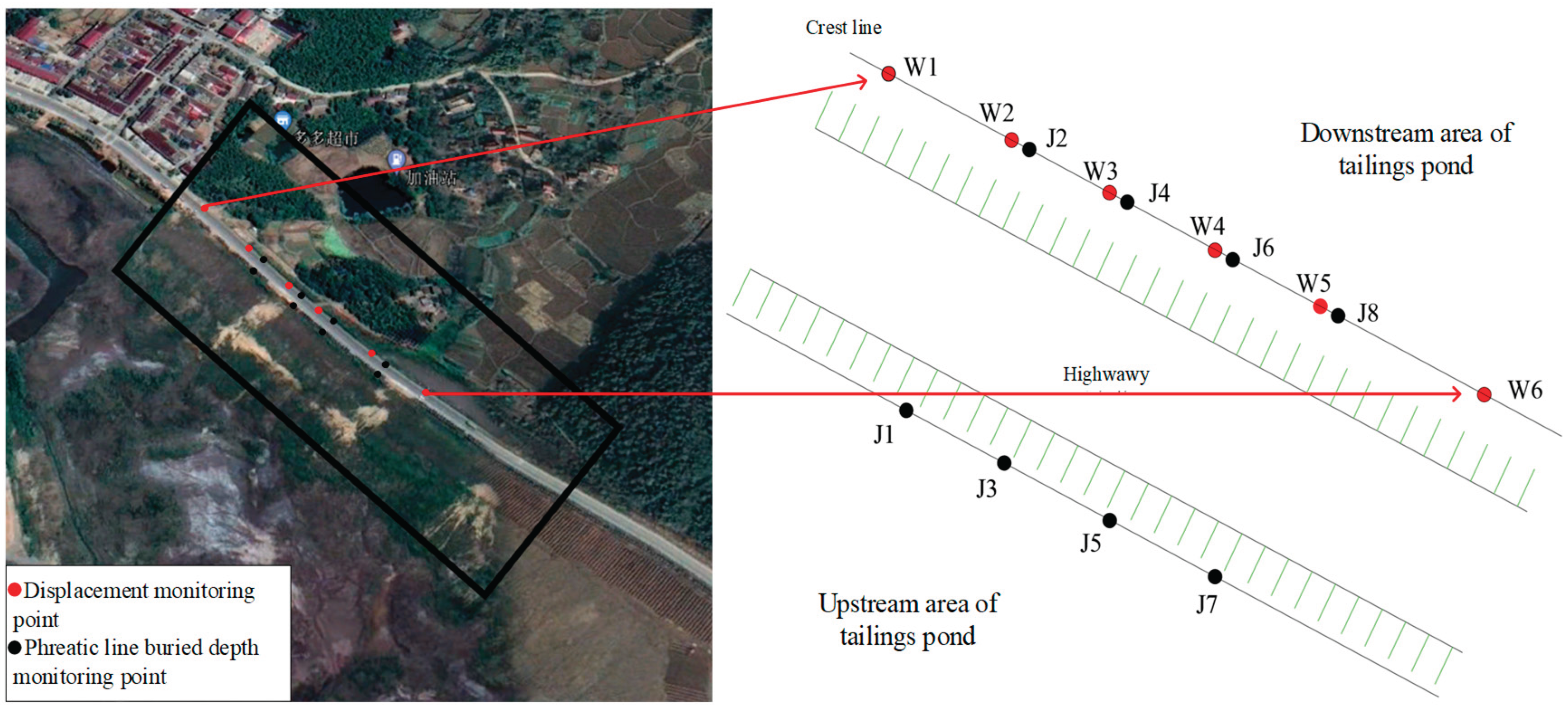
Figure 2.
Data Processing Flow.
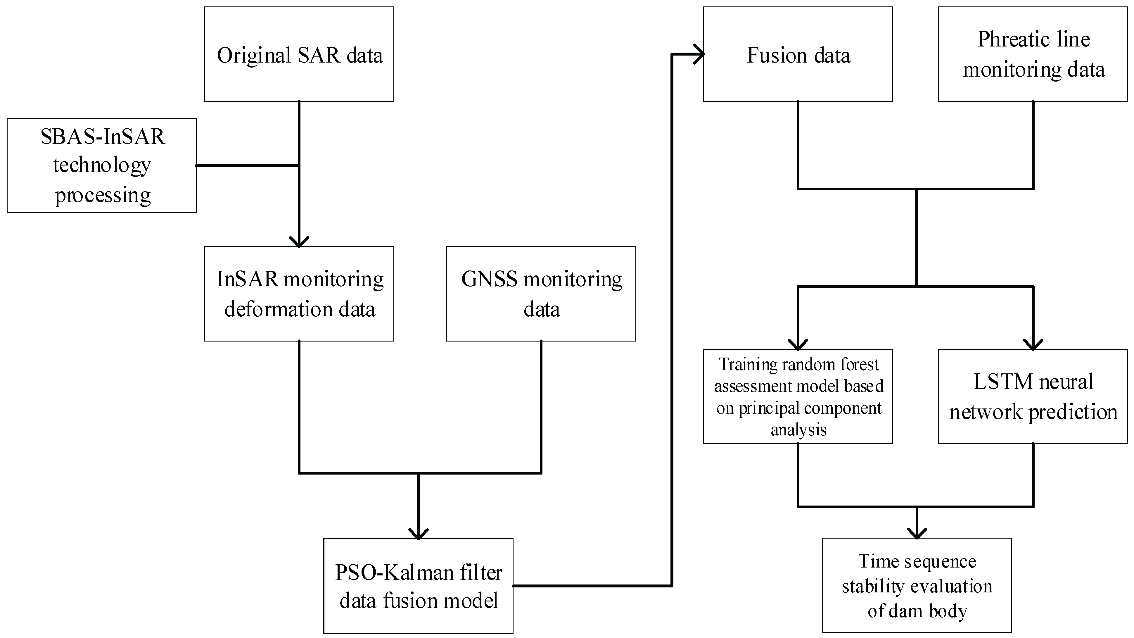
Figure 3.
SBAS-InSAR Data Processing Flow.

Figure 4.
PSO Optimization of Kalman Filter Calculation Process.
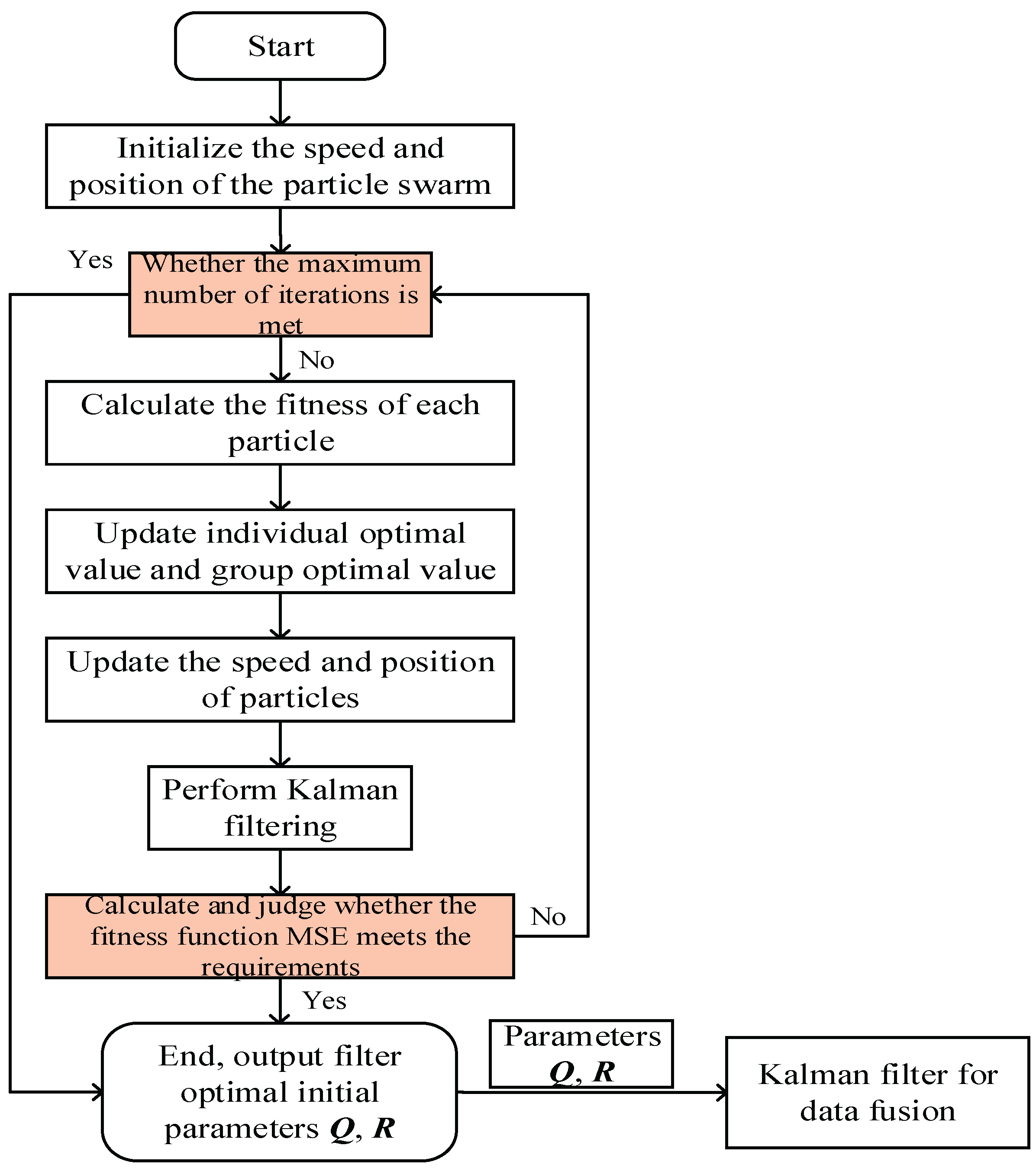
Figure 5.
LSTM Network Structure Diagram.
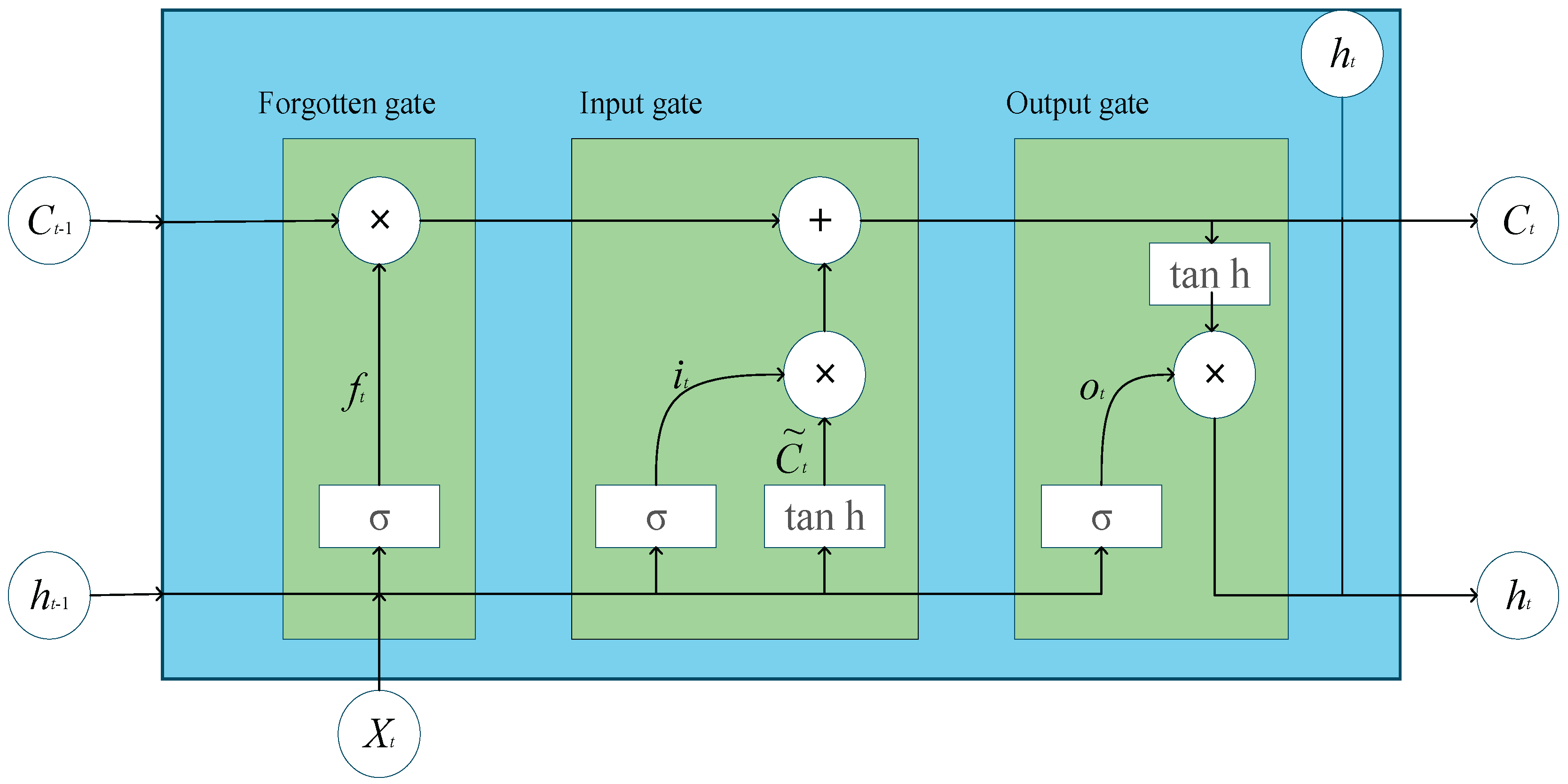
Figure 6.
Network Working Principle.
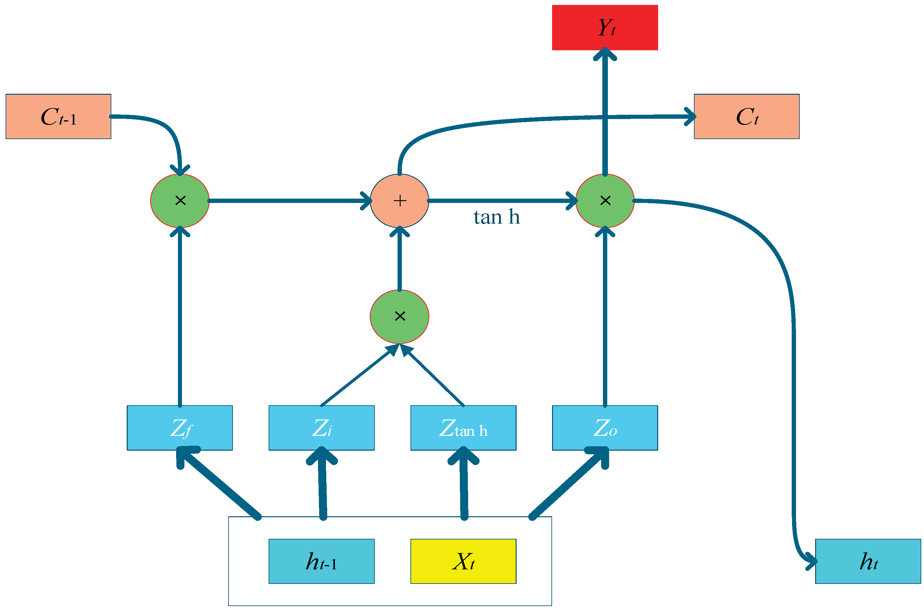
Figure 7.
Random Forest Model.
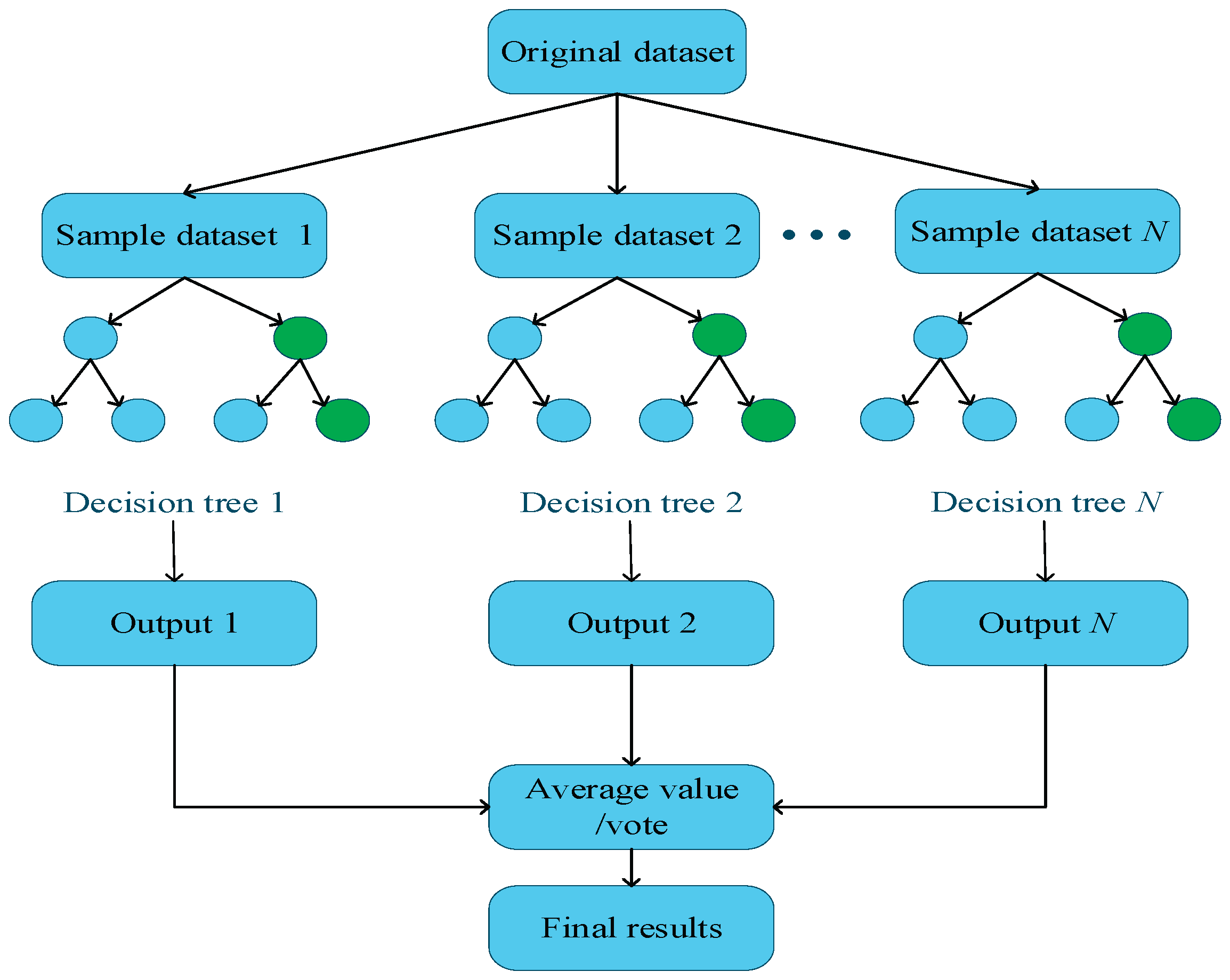
Figure 8.
Comparison between Kalman Filter Algorithm Data Fusion Results and Original Data.
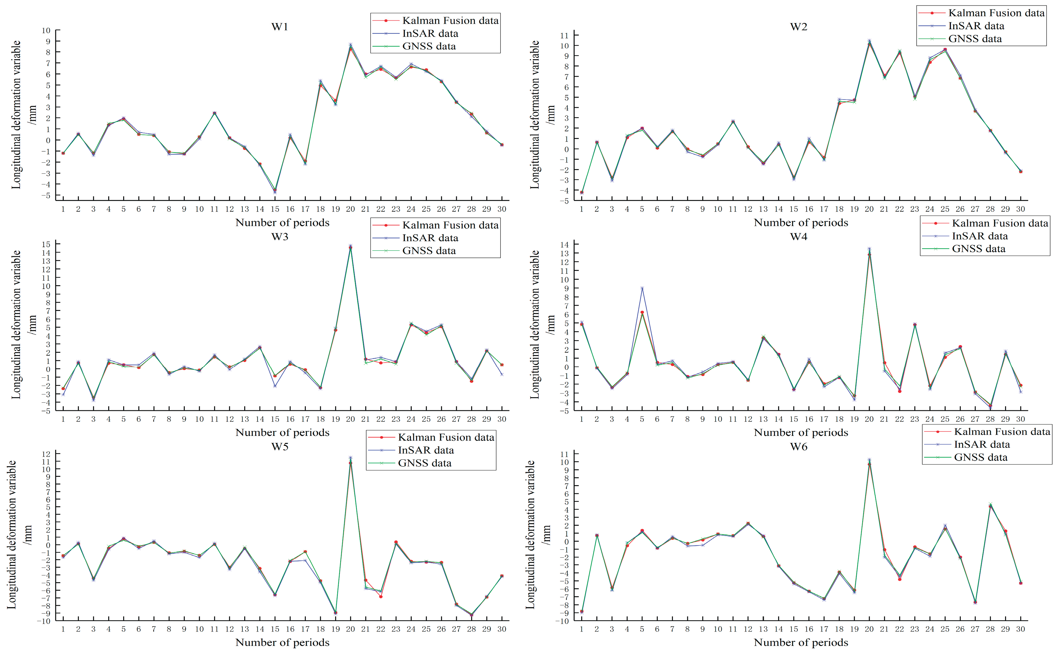
Figure 9.
Comparison between PSO-Kalman Filter Algorithm Data Fusion Results and Original Data.
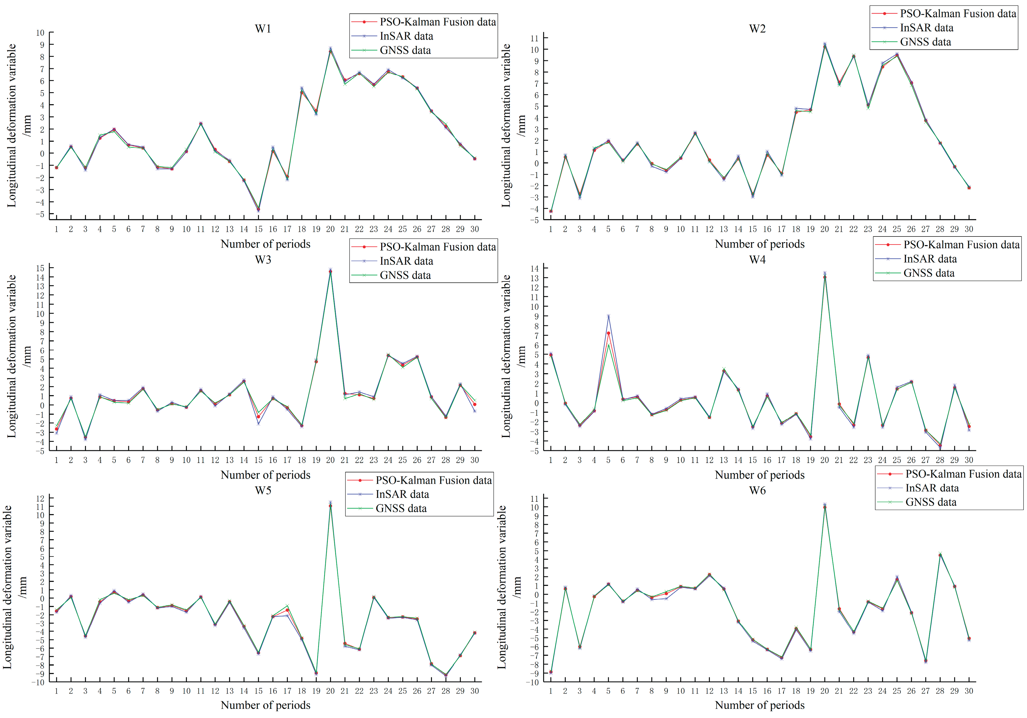
Figure 10.
MAE Comparison Diagram of Two Kalman Filter Fusion Data at Each Monitoring Point.
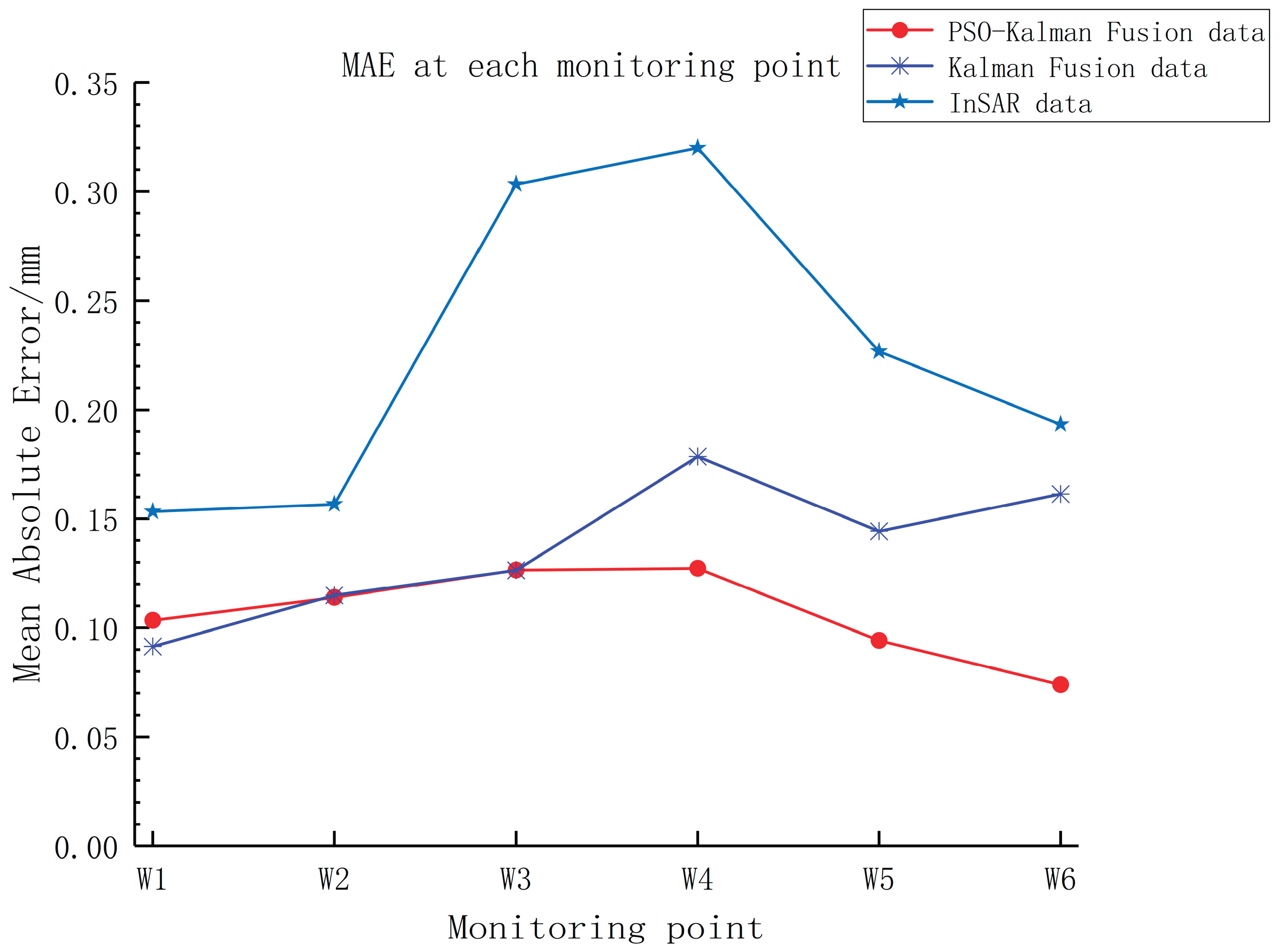
Figure 11.
RMSE Comparison Diagram of Two Kalman Filter Fusion Data at Each Monitoring Point.
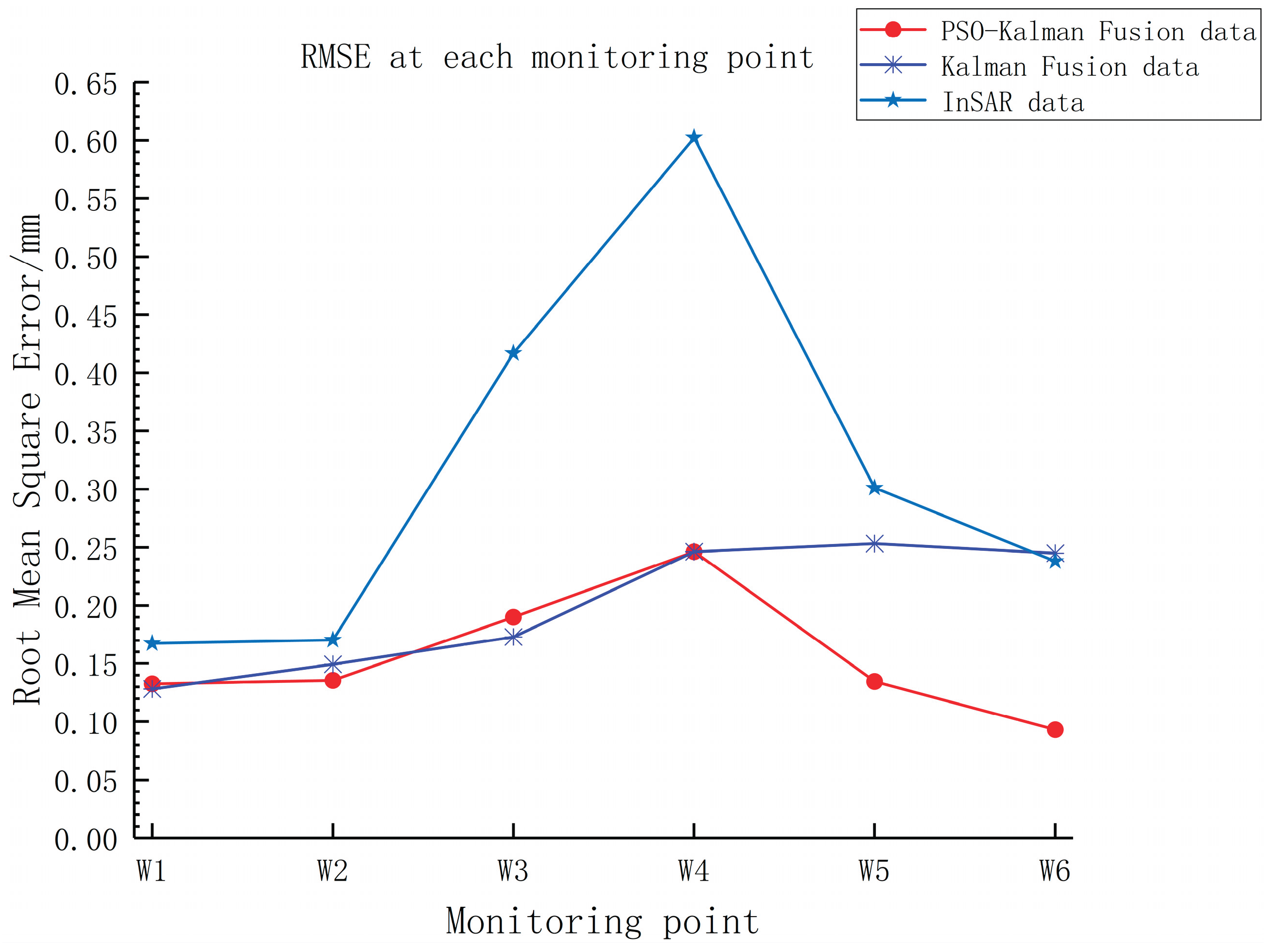
Figure 12.
Comparison Diagram of Predicted Value and Actual Value of Each Monitoring Point.(a) Comparison chart of longitudinal deformation prediction for displacement monitoring points.(b) Comparison chart of buried depth prediction of saturation line monitoring points.
Figure 12.
Comparison Diagram of Predicted Value and Actual Value of Each Monitoring Point.(a) Comparison chart of longitudinal deformation prediction for displacement monitoring points.(b) Comparison chart of buried depth prediction of saturation line monitoring points.
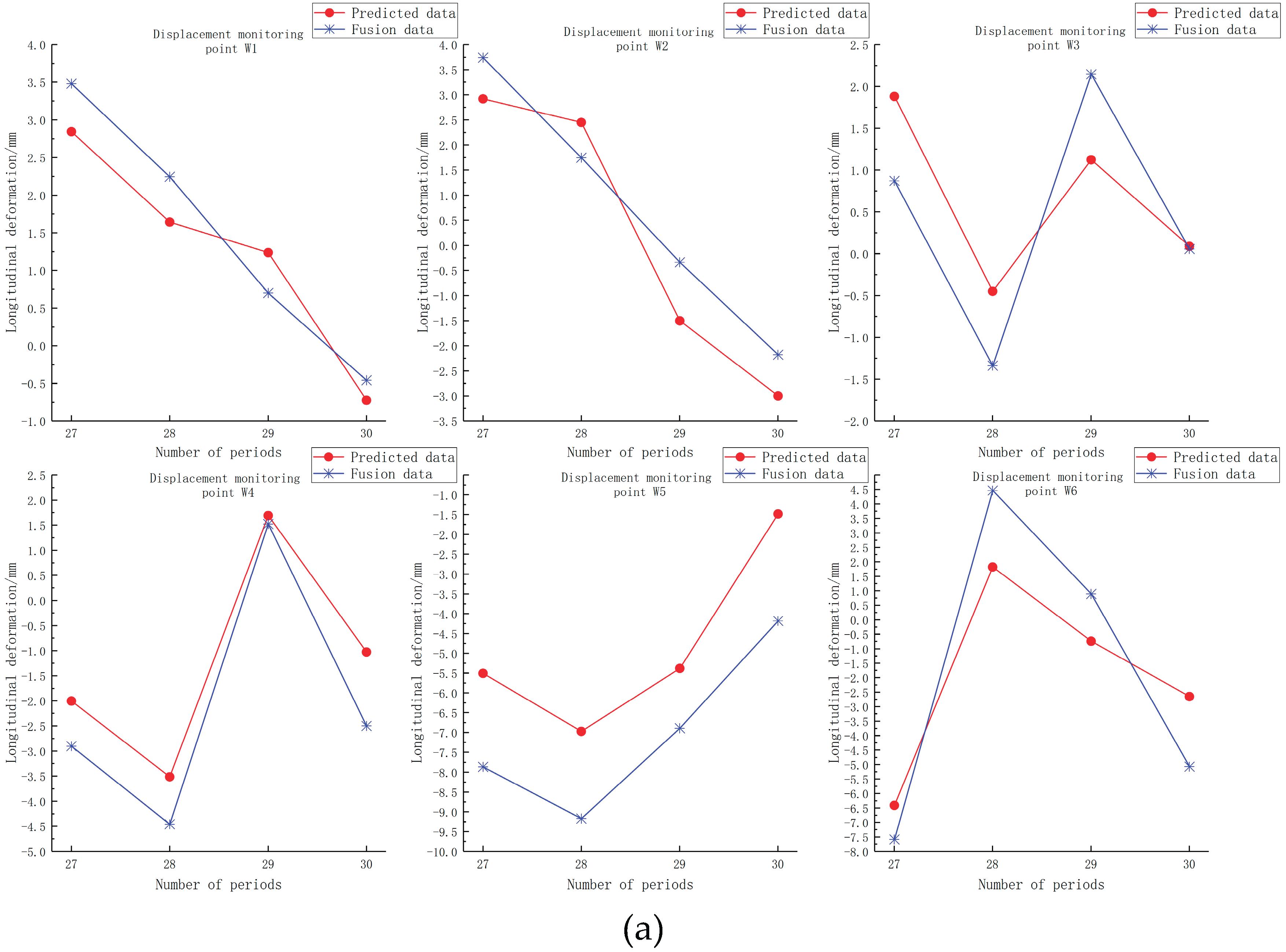
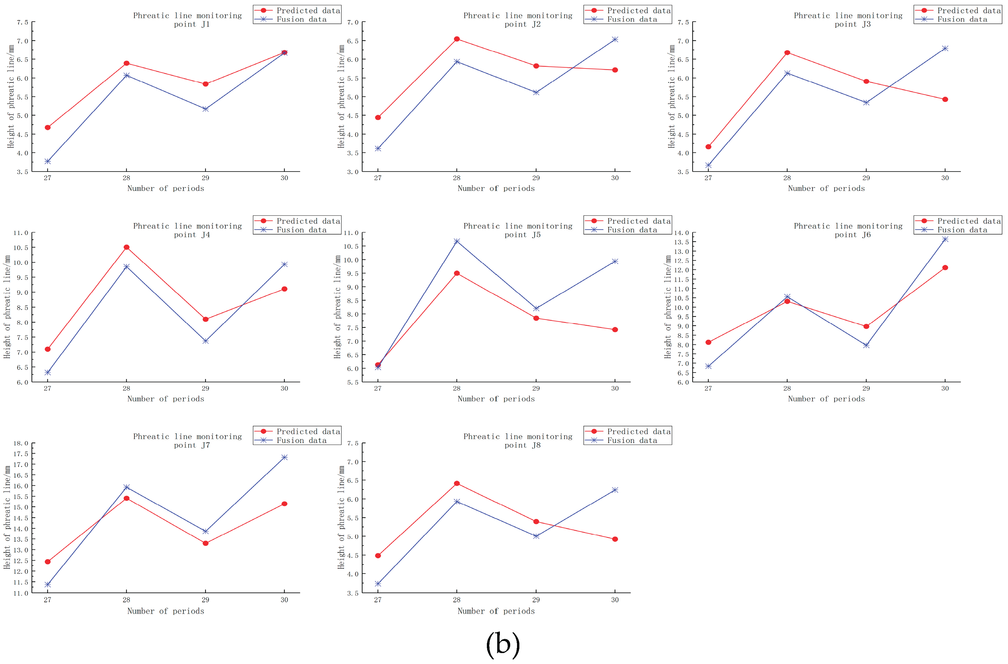
Figure 13.
Schematic Diagram of Principal Component Load.
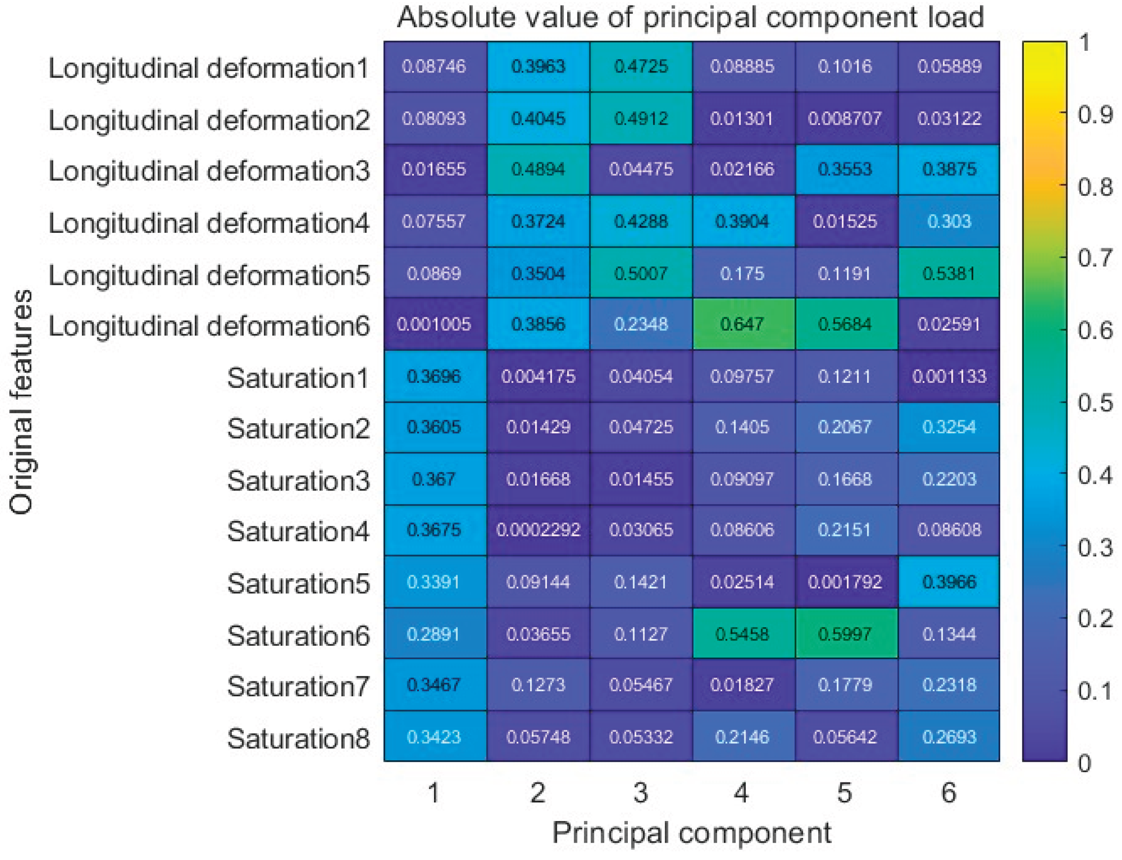
Figure 14.
Confusion matrix of classification verification results.
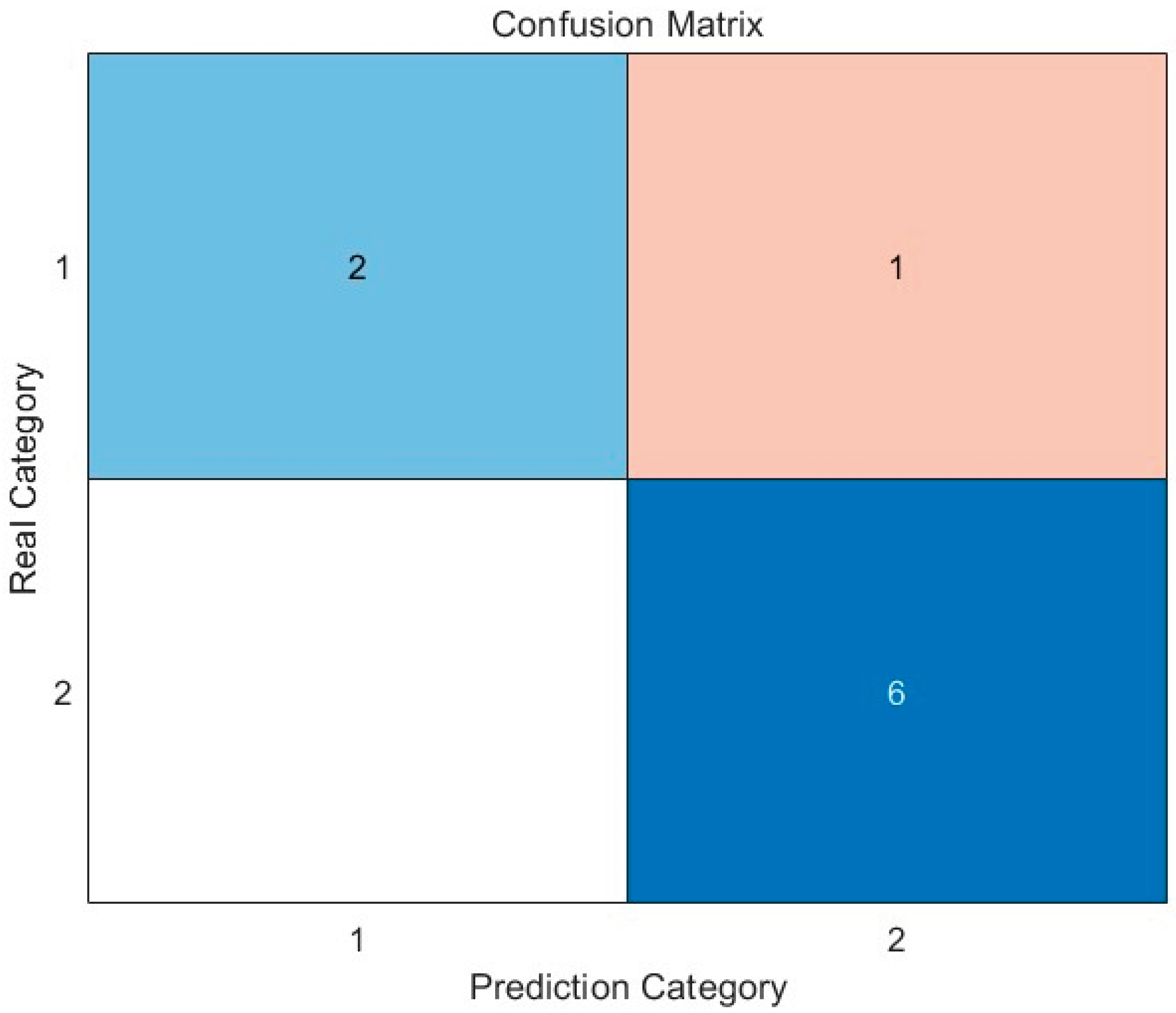
Figure 15.
ROC Curve.
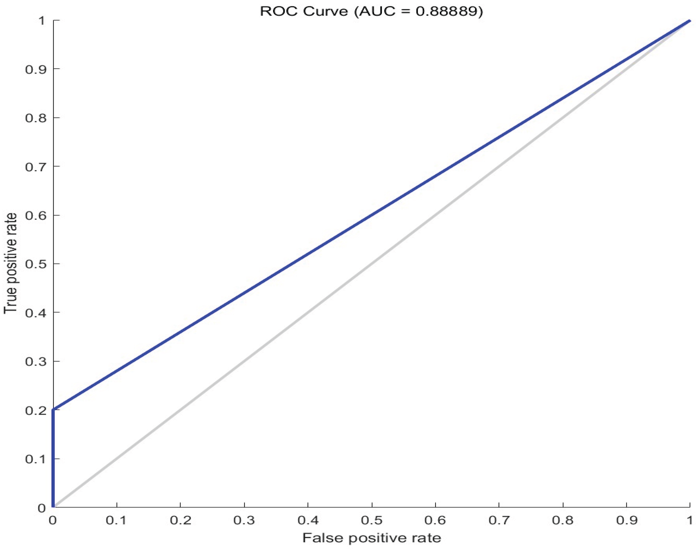

Table 1.
Schematic Diagram of Total MAE and Total RMSE of Fusion Data of Two Kalman Filters.
| Data | MAE/mm | RMSE/mm |
|---|---|---|
| InSAR data | 0.225 6 | 0.351 3 |
| Kalman Fusion data | 0.136 2 | 0.205 5 |
| PSO-Kalman Fusion data | 0.106 6 | 0.163 0 |
Table 2.
Forecast Data RMSE of Each Monitoring Point.
| Monitoring Point | RMSE/mm |
|---|---|
| W1 | 0.5308 |
| W2 | 0.8934 |
| W3 | 0.845 |
| W4 | 0.988 |
| W5 | 2.2364 |
| W6 | 2.0598 |
| J1 | 0.5836 |
| J2 | 0.8197 |
| J3 | 0.745 |
| J4 | 0.8266 |
| J5 | 0.7482 |
| J6 | 1.3973 |
| J7 | 1.123 |
| J8 | 1.2679 |
Table 3.
Prediction Data Sheet of Displacement Monitoring Points.
| Monitoring point | W1 | W2 | W3 | W4 | W5 | W6 |
|---|---|---|---|---|---|---|
| Deformation/mm | 0.3946 | 1.2016 | 1.6078 | 4.5631 | -4.1843 | 0.719 |
Table 4.
Prediction Data Table of Phreatic Line Buried Depth Monitoring Points.
| Monitoring point | J1 | J2 | J3 | J4 | J5 | J6 | J7 | J8 |
|---|---|---|---|---|---|---|---|---|
| Depth and height of infiltration line burial/mm | 4.7675 | 4.2742 | 4.7248 | 4.8631 | 9.4056 | 6.6123 | 9.5643 | 14.254 |
Table 5.
Explain Variance.
| Principal Component | Characteristic Root | Explain Variance | Cumulative Contribution Rate |
|---|---|---|---|
| 1 | 7.0658 | 50.4702% | 50.4702% |
| 2 | 3.3664 | 24.0454% | 74.5156% |
| 3 | 1.5863 | 11.3307% | 85.8463% |
| 4 | 0.6338 | 4.5273% | 90.3736% |
| 5 | 0.4402 | 3.1440% | 93.5176% |
| 6 | 0.3055 | 2.1819% | 95.6995% |
| 7 | 0.2297 | 1.6407% | 97.3402% |
| 8 | 0.1492 | 1.0656% | 98.4057% |
| 9 | 0.1149 | 0.8208% | 99.2265% |
| 10 | 0.038 | 0.2713% | 99.4978% |
| 11 | 0.0304 | 0.2171% | 99.7149% |
| 12 | 0.0199 | 0.1420% | 99.8569% |
| 13 | 0.0115 | 0.0824% | 99.9393% |
| 14 | 0.0085 | 0.0607% | 100.0000% |
Disclaimer/Publisher’s Note: The statements, opinions and data contained in all publications are solely those of the individual author(s) and contributor(s) and not of MDPI and/or the editor(s). MDPI and/or the editor(s) disclaim responsibility for any injury to people or property resulting from any ideas, methods, instructions or products referred to in the content. |
© 2025 by the authors. Licensee MDPI, Basel, Switzerland. This article is an open access article distributed under the terms and conditions of the Creative Commons Attribution (CC BY) license (http://creativecommons.org/licenses/by/4.0/).
Copyright: This open access article is published under a Creative Commons CC BY 4.0 license, which permit the free download, distribution, and reuse, provided that the author and preprint are cited in any reuse.


