Constraint Qualifications and Optimality Criteria for Nonsmooth Multiobjective Mathematical Programming Problems with Equilibrium Constraints on Hadamard Manifolds

1. Introduction

In the theory of mathematical programming, a mathematical programming problem with equilibrium constraints (MPEC) belongs to a special class of constrained optimization problems, characterized by some complementarity or some variational inequality constraints. One of the first attempts in investigating such optimization problems is due to Harker and Pang [20], who explored the existence of efficient solutions for (MPECs). Due to its immense scope of applicability in numerous fields of science, technology, and engineering (see, for instance, [1,8,33]), (MPECs) have been studied by numerous scholars in recent years. For further details and updated survey of (MPEC) and its applications, we refer the readers to [36,37] and the references cited therein.

Optimization in the framework of manifolds has transpired as a very interesting and prominent area of research in the theory of mathematical programming in the last few decades (see, [17,18,40,42] and the references cited therein). The setting of Euclidean geometry has been traditionally employed in data analysis in an extensive manner. In such a setting, the data points have been conveniently represented in terms of coordinates on the Euclidean space by several researchers (see, for instance, [14] and the references cited therein). In recent times, however, researchers have recognized the necessity of employing non-Euclidean geometry, particularly Riemannian geometry, to accurately represent data in more complex models (see, for instance, [5,14] and the references cited therein). Further, in various fields related to engineering, technology, and science, several optimization problems arise which can be formulated in a more effective manner in Riemannian and Hadamard manifold setting, rather than on Euclidean space, see [7,39]. It is worthwhile to note that extending as well as generalizing different techniques involved in optimization theory from the setting of Euclidean spaces to the setting of manifolds result in several crucial advantages. For instance, several complicated constrained mathematical optimization problems can be conveniently converted into unconstrained problems, and thereby the complexity of the original problem can be reduced (see, [11,37] and the references cited therein). Furthermore, many non-convex programming problems can be converted into convex problems by utilizing the Riemannian geometry framework (see, [29,31]). In light of these advantages, various other notions and concepts involved in mathematical programming have been extended from Euclidean spaces to Riemannian and Hadamard manifolds by several researchers (see, for instance, [22,23,41,44,47] and the references cited therein).

Several regularity and optimality criteria for (MPEC) were investigated by Chen and Florian [10]. Abadie constraint qualification for (MPEC) was discussed by Flegel and Kanzow [15]. Various criteria of optimality for (MPEC) were explored by Ye [51]. (GGCQ) as well as criteria of optimality for (MPEC) were explord by Flegel and Kanzow [16]. Optimality conditions for nonsmooth (MPEC) were derived by Ardali et al. [2] using the notion of convexificators. KKT-type criteria for optimality, as well as some duality models for multiobjective (MPEC), were deduced by Singh and Mishra [36]. Pseudonormality, local error bound and Abadie constraint qualification for multiobjective (MPEC) were investigated by Hejazi [21]. Pareto efficiency criteria and some constraint qualifications for smooth multiobjective (MPEC) were discussed by Zhang et al. [52]. Recently, Treanţă et al. [37] studied optimality conditions for multiobjective (MPEC) on Hadamard manifolds.

It is worthwhile to note that optimality conditions for smooth single-objective, as well as multiobjective programming problems in the framework of manifolds, have been studied by several researchers (see, for instance, [6,44] and the references cited therein). Moreover, constraint qualifications such as linearly independent constraint qualification, Mangasarian-Fromovitz constraint qualification, Abadie constraint qualification and Guignard constraint qualification have been studied by Bergmann and Herzog [6] for single-objective problems, and Abadie constraint qualification has been studied by Tung and Tam [38] for multiobjective problems in manifold setting. In sharp contrast to Banach spaces, manifolds, in general, are not equipped with a linear structure. As a result, new approaches are required to deal with nonsmooth functions on manifolds. In this regard, many scholars have recently studied non-smooth analysis on manifolds, see, for instance, [4,19,22,23] and the references cited therein. However, certain important constraint qualifications (such as, Abadie constraint qualification, generalized Abadie constraint qualification, generalized Guignard constraint qualification, Mangasarian-Fromovitz constraint qualification, Cottle constraint qualification, Slater constraint qualification) and optimality criteria for (NMMPEC) have not yet been studied in the setting of Hadamard manifolds using Clarke subdifferentials. The main objective of the present article is to introduce the aforementioned qualifications and further establish optimality criteria for (NMMPEC) on Hadamard manifolds using Clarke subdifferentials.

Motivated by the results established in [10,36,37,51], nonsmooth multiobjective programming problem with equilibrium constraints (NMMPEC) is studied in the present article, in the setting of Hadamard manifolds. Firstly, the generalized Guignard constraint qualification (GGCQ) for (NMMPEC) is introduced in the framework of Hadamard manifolds. We further establish the necessary criteria of Pareto efficiency for (NMMPEC) using (GGCQ). Subsequently, we introduce several (NMMPEC)-tailored constraint qualifications, for instance, Abadie constraint qualification, Cottle-type constraint qualification, Slater-type constraint qualification, and Mangasarian-Fromovitz type constraint qualification in manifold setting. We establish several interesting interrelations between these constraint qualifications. Moreover, we deduce that these constraint qualifications are sufficient conditions for (GGCQ). Non-trivial examples have been incorporated in the setting of some well-known manifolds to justify the importance of the deduced results.

The novelty and the contributions of the present paper are as follows. Firstly, motivated by the results derived by Maeda [27], we introduce several constraint qualifications for (NMPPEC) in the setting of Hadamard manifolds. It is noteworthy that constraint qualifications for (NMPPEC) have not been studied before in manifold setting using Clarke subdifferential. Secondly, the results derived in this article extend the corresponding notions of constraint qualifications studied by Flegel and Kanzow in [15,16] in the setting of more general space, that is, Hadamard manifold, and generalize them for a more general category of optimization problems, that is, (NMMPEC). Moreover, the optimality criteria derived in the present article extend the corresponding results established by Treanţă et al. [37], for a more general category of optimization problems, namely, (NMMPEC).

The rest of the article is organized in the following manner. In Section 2, we recollect some basic concepts and mathematical preliminaries that will be helpful in the sequel. In Section 3, (NMMPEC-GGCQ) is introduced in the setting of Hadamard manifolds, and KKT-type necessary criteria of Pareto efficiency for (NMMPEC) are established. In Section 4, we present several (NMMPEC)-tailored constraint qualifications and establish some interesting interrelations between them. We further establish that these constraint qualifications are sufficient conditions ensuring the satisfaction of (NMMPEC-GGCQ). In Section 5, we draw conclusions to our work in this article and discuss some future research directions.

2. Mathematical Preliminaries and Definitions

The standard symbols ${\mathbb{R}}^n$ and $\mathbb{N}$ are employed to signify the Euclidean space having dimension n and the set of all natural numbers, respectively. The non-negative orthant of ${\mathbb{R}}^n$, denoted by ${\mathbb{R}}_{+}^n$, is defined as:

$${\mathbb{R}}_{+}^n:=\left\{(z_1,z_2,\dots ,z_n):z_k\ge 0,\forall k=1,2,\dots ,n\right\}.$$

We use the symbol $\langle ·,·\rangle$ to signify the usual Euclidean inner product on the set ${\mathbb{R}}^n$. For arbitrary $\alpha ,\beta \in {\mathbb{R}}^n$, the following notation for inequalities will be employed in the sequel:

$$\begin{array}{cc}\hfill \alpha & \prec \beta ⟺{\alpha }_k<{\beta }_k,\forall k=1,2,\dots ,n.\hfill \\ \hfill \alpha & ⪯\beta ⟺\left\{\begin{array}{c}{\alpha }_k\le {\beta }_k,\mathrm{for}\mathrm{all}k=1,2,\dots ,n;k\ne r;\hfill \\ {\alpha }_r<{\beta }_r,\mathrm{for}\mathrm{at}\mathrm{least}\mathrm{one}r\in \{1,2,\dots ,n\}.\hfill \end{array}\right.\hfill \end{array}$$

Let ${\mathcal{H}}_n$ signify any n-dimensional Riemannian manifold. Then, ${\mathcal{H}}_n$ is termed as a Hadamard manifold if ${\mathcal{H}}_n$ is geodesic complete, simply connected, as well as the sectional curvature of ${\mathcal{H}}_n$ is non-positive everywhere. From now onwards, in this article, the symbol ${\mathcal{H}}_n$ will always indicate a Hadamard manifold having dimension n, unless it is mentioned otherwise.

Let $\widehat{a}\in {\mathcal{H}}_n$. The tangent space at the point $\widehat{a}$ is denoted by $T_{\widehat{a}}{\mathcal{H}}_n$. The exponential mapping defined on the tangent space ${\exp }_{\widehat{a}}:T_{\widehat{a}}{\mathcal{H}}_n\to {\mathcal{H}}_n$ is a globally diffeomorphic map. Further, ${\exp }_{\widehat{a}}^{-1}:{\mathcal{H}}_n\to T_{\widehat{a}}{\mathcal{H}}_n$ satisfies ${\exp }_{\widehat{a}}^{-1}\left(\widehat{a}\right)=0$. For every ${\widehat{a}}_1,{\widehat{a}}_2\in {\mathcal{H}}_n$, some unique normalized minimal geodesic ${\mathsf{\nu }}_{{\widehat{a}}_1,{\widehat{a}}_2}:[0,1]\to {\mathcal{H}}_n$ always exists, such that ${\mathsf{\nu }}_{{\widehat{a}}_1,{\widehat{a}}_2}\left(\mathsf{\tau }\right)={\exp }_{{\widehat{a}}_1}\left(\mathsf{\tau }{\exp }_{{\widehat{a}}_1}^{-1}\left({\widehat{a}}_2\right)\right),\forall \mathsf{\tau }\in [0,1].$ It is a well-known fact that ${\mathcal{H}}_n$ is diffeomorphic to the n-dimensional Euclidean space ${\mathbb{R}}^n$. For any differentiable function $\mathcal{W}:{\mathcal{H}}_n\to \mathbb{R}$, the gradient of $\mathcal{W}$, denoted by grad $\mathcal{W}$, is a vector field on the manifold ${\mathcal{H}}_n$ defined through $d\mathcal{W}\left(X\right)=\langle grad\mathcal{W},X\rangle =X\left(\mathcal{W}\right)$, where X is a vector field on ${\mathcal{H}}_n$.

Now, we recall the definition of locally Lipschitz function in the setting of Hadamard manifolds (see, for instance, [23]).

Definition 1.

Let $\mathcal{G}\subseteq {\mathcal{H}}_n$ and $\mathcal{W}:\mathcal{G}\to \mathbb{R}$ be a real-valued function. Then $\mathcal{W}$ is referred to as locally Lipschitz at $z\in \mathcal{G}$ with rank $\mathcal{L}$ ($\mathcal{L}\in \mathbb{R}$, $\mathcal{L}>0$), if for every $z_1,z_2$ lying in some open neighborhood of z, the following is satisfied:

$$|\mathcal{W}\left(z_1\right)-\mathcal{W}\left(z_2\right)|\le K\omega (z_1,z_2),$$

where $\omega (z_1,z_2)$ is the Riemannian distance between the points $z_1$ and $z_2$ on $\mathcal{G}$.

Remark 1. 

(a) If $\mathcal{W}$ is locally Lipschitz at every element $z\in \mathcal{G}$, then $\mathcal{W}$ is said to be locally Lipschitz on the set $\mathcal{G}$.

(b) 

It is significant to observe that several functions which are not locally Lipschitz in Euclidean space setting, can be locally Lipschitz in the setting of Hadamard manifolds. For instance, let us consider the set $\mathcal{H}$ defined as:

$$\mathcal{H}:=\{z=(z_2,z_2)\in {\mathbb{R}}^2:z_1>0,z_2>0\}.$$

Consider the real-valued function $\mathcal{W}:\mathcal{H}\to \mathbb{R}$ defined as follows:

$$\mathcal{W}\left(z\right)=\sum _{i=1}^{2}ln\left(z_i\right),$$

for every $z=\left(z_1,z_2\right)\in \mathcal{H}$. One can verify that the function $\mathcal{W}$ is not a locally Lipschitz function on the set $\mathcal{H}$ in the usual Euclidean sense. However, $\mathcal{H}$ can be considered as a Hadamard manifold by endowing it with the Riemannian metric given by

$${\langle u,v\rangle }_y=\langle \mathcal{G}\left(y\right)u,v\rangle ,\forall u,v\in T_y\mathcal{H}={\mathbb{R}}^2,y\in \mathcal{H},$$

where the symbol $\langle ·,·\rangle$ denotes the Euclidean inner product on ${\mathbb{R}}^2$ and

$$\mathcal{G}\left(y\right)=\left(\begin{array}{cc}{\displaystyle \frac{1}{y_1^2}}& 0\\ 0& {\displaystyle \frac{1}{y_2^2}}\end{array}\right).$$

Then, it can be verified that the function $\mathcal{W}$ is locally Lipschitz with rank 1 on the set $\mathcal{H}$ in the setting of manifolds (see, for instance, [12]).

The following definition is from Udrişte [39].

Definition 2.

Let $\mathcal{D}\subseteq {\mathcal{H}}_n$ be non-empty. Then, $\mathcal{D}$ is termed as a geodesic convex set in ${\mathcal{H}}_n$, if for every $y,\tilde{y}\in \mathcal{D}$, there exists some unique minimal geodesic ${\gamma }_{y,\tilde{y}}:[0,1]\to {\mathcal{H}}_n$ joining the points y and $\tilde{y}$. That is, we have

$${\gamma }_{y,\tilde{y}}\left(t\right)\in \mathcal{D},\forall t\in [0,1].$$

The following definitions are from Barani [4].

Definition 3.

Let $\mathcal{F}:{\mathcal{H}}_n\to \mathbb{R}$ be a real-valued and locally Lipschitz function. Let $x,y\in {\mathcal{H}}_n$ be arbitrary elements. Then, the generalized directional derivative of $\mathcal{F}$ at y in the direction $v\in T_y{\mathcal{H}}_n$, is denoted by the symbol ${\mathcal{F}}^{\circ }(y;v)$, and is defined as follows:

$${\mathcal{F}}^{\circ }(y;v):=\underset{x\to y,t\downarrow 0}{lim\; sup}{\displaystyle \frac{\mathcal{F}\left({exp}_{x}t{\left(d{exp}_y\right)}_{{exp}_y^{-1}x}v\right)-\mathcal{F}\left(x\right)}{t}},$$

where ${\left(d{exp}_y\right)}_{{exp}_y^{-1}x}:T_{{exp}_y^{-1}x}\left(T_y{\mathcal{H}}_n\right)\simeq T_y{\mathcal{H}}_n\to T_x{\mathcal{H}}_n$ is the differential of the exponential function at ${exp}_y^{-1}x$.

Definition 4.

Let $\mathcal{F}:{\mathcal{H}}_n\to \mathbb{R}$ be a real-valued and locally Lipschitz function. Then, the Clarke subdifferential of $\mathcal{F}$ at $y\in {\mathcal{H}}_n$, denoted by ${\partial }^c\mathcal{F}\left(y\right)$, is defined by

$${\partial }^c\mathcal{F}\left(y\right):=\left\{\mathsf{\zeta }\in T_y{\mathcal{H}}_n\mid {\mathcal{F}}^{\circ }(y;v)\ge \langle \mathsf{\zeta },v\rangle ,\forall v\in T_y{\mathcal{H}}_n\right\}.$$

The following lemma will be useful in the sequel (see, [23]).

Lemma 1.

Let $\mathcal{F}:{\mathcal{H}}_n\to \mathbb{R}$ be a real-valued and locally Lipschitz function with Lipschitz constant $\mathcal{L}$ near $y\in {\mathcal{H}}_n$. Then

(a) 

The Clarke subdifferential ${\partial }^c\mathcal{F}\left(y\right)$ is a nonempty, convex, compact subset of $T_y{\mathcal{H}}_n$. Moreover, $\parallel \mathsf{\zeta }\parallel \le \mathcal{L}$ for $every\mathsf{\zeta }\in {\partial }^c\mathcal{F}\left(y\right)$, and ${\partial }^c\mathcal{F}\left(y\right)$ is upper semicontinuous at y.

(b) 

For every w in $T_y{\mathcal{H}}_n$ we have

$${\mathcal{F}}^{\circ }(y;w)=max\{\langle \mathsf{\zeta },w\rangle :\mathsf{\zeta }\in {\partial }^c\mathcal{F}\left(y\right)\}.$$

(c) 

If $\left\{y_n\right\}$ and $\left\{{\mathsf{\zeta }}_n\right\}$ are sequences in ${\mathcal{H}}_n$ and the tangent bundle $T{\mathcal{H}}_n$, respectively, such that ${\mathsf{\zeta }}_n\in {\partial }^c\mathcal{F}\left(y_n\right)$ for every $n\in \mathbb{N}$, $\left\{y_n\right\}\to y$. Further, let $\mathsf{\zeta }$ be a weak*-cluster point of $\left\{{\mathcal{P}}_{y_n}^y{\mathsf{\zeta }}_n\right\}$. Then, we have $\mathsf{\zeta }\in {\partial }^c\mathcal{F}\left(y\right)$.

Now, we recall the following lemma from Grohs and Hosseini [19].

Lemma 2.

Let $\mathcal{F}:{\mathcal{H}}_n\to \mathbb{R}$ be a real-valued and locally Lipschitz function. Let ${\mathcal{D}}_{\mathcal{W}}$ be the set of all points at which the function $\mathcal{F}$ is differentiable on ${\mathcal{H}}_n$. Then, ${\mathcal{D}}_{\mathcal{F}}$ is dense in ${\mathcal{H}}_n$, and

$${\partial }^c\mathcal{F}\left(y\right)=co\left\{\underset{n\to \infty }{lim}grad\left(y_n\right):\left\{y_n\right\}\subseteq {\mathcal{D}}_{\mathcal{F}},y_n\to y\right\}.$$

The following definition is taken from Barani [4].

Definition 5.

Let $\mathcal{F}:\mathcal{D}\to \mathbb{R}$ be a real-valued and locally Lipschitz function defined on a geodesic convex subset $\mathcal{D}$ of the Hadamard manifold ${\mathcal{H}}_n$. Then, $\mathcal{F}$ is referred to as a geodesic convex function at $\widehat{x}$, provided that for every $x\in \mathcal{D}$ and for every $\mathsf{\zeta }\in {\partial }^c\mathcal{F}\left(\widehat{x}\right)$ we have

$$\mathcal{F}\left(x\right)-\mathcal{F}\left(\widehat{x}\right)\ge {〈\mathsf{\zeta },{exp}_{\widehat{x}}^{-1}x〉}_{\widehat{x}}.$$

The function $\mathcal{F}$ is termed as a geodesic strictly convex function at $\widehat{x}\in \mathcal{D}$, provided that the preceding inequality holds strictly, for $\widehat{x}\ne x$. The function $\mathcal{F}$ is termed as a geodesic (strictly) concave function at $\widehat{x}\in \mathcal{D}$, provided that $-\mathcal{F}$ is geodesic (strictly) convex at $\widehat{x}\in \mathcal{D}$. A function that is both geodesic convex and geodesic concave at $\widehat{x}\in \mathcal{D}$ is said to be a geodesic affine function $\widehat{x}\in \mathcal{D}$.

Remark 2.

It is worthwhile to note that several nonconvex functions in Euclidean space settings can be suitably transformed into geodesic convex functions in the framework of manifolds. As a result, a wider range of optimization problems can be explored by formulating the problems in manifold settings. For instance, consider the set $\mathcal{D}\subset {\mathbb{R}}^2$ defined in the following manner:

$$\mathcal{D}:=\left\{\left(y_1,y_2\right)\in {\mathbb{R}}^2:y_2=y_1^2,y_1\in \left[{\displaystyle \frac{1}{2}},1\right]\right\}.$$

Let us now consider the function $\mathcal{F}:\mathcal{D}\times \mathcal{D}\to \mathbb{R}$ defined in the following manner:

$$\mathcal{F}(x,y)=y_1^2-y_1^4+y_2+y_2^2-x_1^2-x_2,$$

for every $x=(x_1,x_2)$ and $y=(y_1,y_2)$ in $\mathcal{D}$. By elementary calculations, one can verify that the set $\mathcal{D}$ is not a convex set in the Euclidean space in the usual sense.

However, one can view the set $\mathcal{D}$ as the image of a geodesic segment on the paraboloid of revolution $P(u_1,u_2)=$$\left(u_{2}cos{u}_1,u_{2}sin{u}_1,u_2^2\right)$, $u_1,u_2\in \mathcal{D}$, which is endowed with the Riemannian metric $\mathcal{G}$, given by:

$$\mathcal{G}(u_1,u_2)=\left(\begin{array}{cc}{u}_2^2& 0\\ 0& 1+4u_2^2\end{array}\right).$$

It can be verified that the set $\mathcal{D}$ is a geodesic convex set on the Riemannian manifold formed by the image of the paraboloid of revolution (see, for instance, [25]). Furthermore, the function $\mathcal{F}(x,·)$ is not a convex function in the Euclidean space setting. However, $\mathcal{F}(x,·)$ is a geodesic convex function on the set $\mathcal{D}$.

The following theorem is an extension of Lebourg’s mean value theorem on Hadamard manifolds (see, for instance, [4]).

Theorem 1.

Let $\mathcal{F}:{\mathcal{H}}_n\to \mathbb{R}$ be a ral valued and locally Lipschitz function. Then, for every $x,y\in {\mathcal{H}}_n$, there exist $t_0\in (0,1)$ and $z_0=\rho \left(t_0\right)$, such that

$$\mathcal{F}\left(y\right)-\mathcal{F}\left(x\right)\in 〈{\partial }^c\mathcal{F}\left(z_0\right),{\rho }^{\prime }\left(t_0\right)〉,$$

where $\rho \left(t\right):={exp}_x\left(t{exp}_x^{-1}\left(y\right)\right)$ and $t\in [0,1]$.

The following lemma from [46] is an extension of Motzkin’s theorem of alternative in the setting of Hadamard manifolds.

Lemma 3.

Let $p\in {\mathcal{H}}_n$ and A, B, C be matrices of order $m_1\times n$, $m_2\times n$ and $m_3\times n$, respectively, such that every row of A, B and C is a tangent vector at p, that is, $A_i\in T_p{\mathcal{H}}_n$, for every $i=1,2,\dots ,m_1$, $B_j\in T_p{\mathcal{H}}_n$, for every $j=1,2,\dots ,m_2$ and $C_k\in T_p{\mathcal{H}}_n$, for every $k=1,2,\dots ,m_3$. Then, exactly one of the following assertions (but not both) holds true:

(a) 

The system of inequalities:

$$\begin{array}{cccc}\hfill {\langle A_i,x\rangle }_p& >0,\hfill & \hfill & \forall i=1,2,\dots ,m_1,\hfill \\ \hfill {\langle B_j,x\rangle }_p& \ge 0,\hfill & \hfill & \forall j=1,2,\dots ,m_2,\hfill \\ \hfill {\langle C_k,x\rangle }_p& =0,\hfill & \hfill & \forall k=1,2,\dots ,m_3,\hfill \end{array}$$

has a solution $x\in T_p{\mathcal{H}}_n$;

(b) 

The following equation:

$$A^T{z}_1+B^T{z}_2+c^T{z}_3=0,$$

has a solution $z_1\in {\mathbb{R}}^{m_1}$, $z_2\in {\mathbb{R}}^{m_2}$, $z_3\in {\mathbb{R}}^{m_3}$, such that $z_1\ge 0$, $z_2\geqq 0$.

For more comprehensive discussions on Riemannian manifolds, we refer to [28,34,39,43,48,49,50] and the references cited therein.

3. Constraint Qualifications and Necessary Optimality Criteria for (NMMPEC)

In this section, a nonsmooth multiobjective programming problem with equilibrium constraints (NMMPEC) is considered in the setting of Hadamard manifolds. We deduce KKT type necessary criteria of Pareto efficiency for (NMMPEC) by employing the generalized Guignard constraint qualification.

Let us consider the following (NMMPEC) in the setting of Hadamard manifolds:

$$\begin{array}{c}\hfill \left(\mathrm{NMMPEC}\right)\mathrm{Minimize}\mathcal{F}\left(y\right):=\left({\mathcal{F}}_1\left(y\right),{\mathcal{F}}_2\left(y\right),\dots ,{\mathcal{F}}_r\left(y\right)\right)\end{array}$$

$$\begin{array}{cccc}\hfill \mathrm{subject}\mathrm{to}{\mathcal{W}}_j\left(y\right)& \le 0,\hfill & \hfill & \forall j\in {\mathcal{I}}^{\mathcal{W}}:=\{1,2,\dots ,l\},\hfill \\ \hfill {\mathcal{V}}_j\left(y\right)& =0,\hfill & \hfill & \forall j\in {\mathcal{I}}^{\mathcal{V}}:=\{1,2,\dots ,p\},\hfill \\ \hfill {\mathcal{C}}_j\left(y\right)& \ge 0,\hfill & \hfill & \forall j\in \mathcal{T}:=\{1,2,\dots ,m\},\hfill \\ \hfill {\mathcal{D}}_j\left(y\right)& \ge 0,\hfill & \hfill & \forall j\in \mathcal{T},\hfill \\ \hfill {\mathcal{D}}_j\left(y\right){\mathcal{C}}_j\left(y\right)& =0,\hfill & \hfill & \forall j\in \mathcal{T},\hfill \end{array}$$

where each of the functions ${\mathcal{F}}_j:{\mathcal{H}}_n\to \mathbb{R}$ ($j\in \mathcal{I}:=\{1,2,\dots ,r\})$, ${\mathcal{W}}_j:{\mathcal{H}}_n\to \mathbb{R}$, ($j\in {\mathcal{I}}^{\mathcal{W}}$), ${\mathcal{V}}_j:{\mathcal{H}}_n\to \mathbb{R}$ ($j\in {\mathcal{I}}^{\mathcal{V}}$), ${\mathcal{C}}_j:{\mathcal{H}}_n\to \mathbb{R}$, ${\mathcal{D}}_j:{\mathcal{H}}_n\to \mathbb{R}$ ($j\in \mathcal{T}$) are assumed to be locally Lipschitz and are defined on some Hadamard manifold ${\mathcal{H}}_n$ having dimension n, where $n\in \mathbb{N}$.

Let $\mathcal{S}$ be the set containing every feasible solution of the considered problem (NMMPEC).

We recall the concepts of Pareto efficiency as well as weak Pareto efficiency in the following definitions, which will be used in the paper (for instance, see, [27]).

Definition 6.

Let $\widehat{z}\in \mathcal{S}$ be arbitrary. Then $\widehat{z}$ is termed as a Pareto efficient solution of (NMMPEC), provided that there does not exist any other feasible element $\tilde{z}\in \mathcal{S}$ which satisfies the following inequality:

$$\begin{array}{cc}\hfill \mathcal{F}\left(\tilde{z}\right)& ⪯\mathcal{F}\left(\widehat{z}\right).\hfill \end{array}$$

Definition 7.

Let $\widehat{z}\in \mathcal{S}$ be arbitrary. Then $\widehat{z}$ is termed as a weak Pareto efficient solution of (NMMPEC), provided that there does not exist any other feasible element $\tilde{z}\in \mathcal{S}$ which satisfies the following inequality:

$$\begin{array}{cc}\hfill \mathcal{F}\left(\tilde{z}\right)& \prec \mathcal{F}\left(\widehat{z}\right).\hfill \end{array}$$

Suppose that $\widehat{z}\in \mathcal{S}$ is any arbitrary feasible solution of (NMMPEC). The index sets defined below will be crucial in the remaining part of the article.

$$\begin{array}{cc}\hfill {\mathcal{A}}^{\mathcal{W}}\left(\widehat{z}\right)& :=\{j\in {\mathcal{I}}^{\mathcal{W}}:{\mathcal{W}}_j\left(\widehat{z}\right)=0\},\hfill \\ \hfill {\mathcal{R}}_{+0}\left(\widehat{z}\right)& :=\left\{j\in \mathcal{T}:{\mathcal{C}}_j\left(\widehat{z}\right)>0,{\mathcal{D}}_j\left(\widehat{z}\right)=0\right\},\hfill \\ \hfill {\mathcal{R}}_{0+}\left(\widehat{z}\right)& :=\left\{j\in \mathcal{T}:{\mathcal{C}}_j\left(\widehat{z}\right)=0,{\mathcal{D}}_j\left(\widehat{z}\right)>0\right\},\hfill \\ \hfill {\mathcal{R}}_{00}\left(\widehat{z}\right)& :=\left\{j\in \mathcal{T}:{\mathcal{C}}_j\left(\widehat{z}\right)=0,{\mathcal{D}}_j\left(\widehat{z}\right)=0\right\}.\hfill \end{array}$$

Remark 3. 

(a) The index set $\mathcal{A}\left(\widehat{z}\right)$ is termed as the set of all active inequality indices for the function $\mathcal{W}$ at the point $\widehat{z}$.

(b) 

The index set ${\mathcal{R}}_{00}\left(\widehat{z}\right)$ is termed as the degenerate index set at the point $\widehat{z}$. The strict complementarity condition is said to be satisfied at $\widehat{z}$ provided that ${\mathcal{R}}_{00}\left(\widehat{z}\right)=\varnothing$.

(b) 

One can observe the fact that every index set that is defined above is dependent on the particular choice of $\widehat{z}\in \mathcal{S}$. Nevertheless, in the remaining part of the article, we shall not indicate such dependence explicitly when it will be easily perceivable from the context.

Let $\tilde{y}\in \mathcal{S}$ be arbitrary. The sets ${\mathcal{L}}^k$ (for every $k\in \mathcal{I}$) and $\mathcal{L}$ as defined below will be crucial to discuss Guignard constraint qualification and optimality conditions for (NMMPEC).

$$\begin{array}{cc}\hfill {\mathcal{L}}^k& :=\left\{y\in \mathcal{S}:{\mathcal{F}}_j\left(y\right)\le {\mathcal{F}}_j\left(\tilde{y}\right),\forall j\in \mathcal{I},j\ne k\right\},\hfill \\ \hfill \mathcal{L}& :=\left\{y\in \mathcal{S}:{\mathcal{F}}_j\left(y\right)\le {\mathcal{F}}_j\left(\tilde{y}\right),\forall j\in \mathcal{I}\right\}.\hfill \end{array}$$

Remark 4. 

(a) From the above definitions of the sets ${\mathcal{L}}^k$ and $\mathcal{L}$ it is clear that

$$\bigcap _{k\in \mathcal{I}}{\mathcal{L}}^k=\mathcal{L}.$$

(b) 

In case $\mathcal{I}=\left\{1\right\}$, then (NMMPEC) reduces to a nonsmooth single-objective optimization problem with equilibrium constraints. Then

$${\mathcal{L}}^1=\mathcal{S}.$$

In the next definition, we recall the notion of the contingent cone for any subset of ${\mathcal{H}}_n$ (see, [24]).

Definition 8.

Let $\mathcal{D}\subseteq {\mathcal{H}}_n$ and $a^{*}$ be some arbitrary element in the closure of the set $\mathcal{D}$. Then the contingent cone (in other terms, Bouligand tangent cone) of the set $\mathcal{D}$ at the element $a^{*}$ is symbolized by the notation ${\mathcal{C}}^{Tan}(\mathcal{D},a^{*})$ and is given by:

$$\begin{array}{cc}\hfill {\mathcal{C}}^{Tan}(\mathcal{D},a^{*}):=\{\widehat{w}\in T_{a^{*}}{\mathcal{H}}_n:\exists {\sigma }_n\downarrow 0,\exists {\left\{{\widehat{w}}_n\right\}}_{n=1}^{\infty }& \subset T_{a^{*}}{\mathcal{H}}_n,{\widehat{w}}_n\to \widehat{w},\hfill \\ & {\exp }_{a^{*}}\left({\sigma }_n{\widehat{w}}_n\right)\in \mathcal{D}\forall n\in \mathbb{N}\}.\hfill \end{array}$$

With the aim to introduce (GGCQ) for our considered problem (NMMPEC), we now define the notion of (NMMPEC)-tailored linearizing cone in manifold setting using Clarke subdifferential.

Definition 9.

Let $a^{*}\in \mathcal{S}$ be arbitrary. The (NMMPEC)-tailored linearizing cone to $\mathcal{L}$ at the element $a^{*}$ is the set defined as follows:

$$\begin{array}{cccccc}\hfill {\mathcal{C}}_{MMPEC}^{Lin}\left(\mathcal{L},a^{*}\right):=\{\overline{u}\in T_{a^{*}}{\mathcal{H}}_n:& \langle {\mathsf{\zeta }}_j^{\mathcal{F}},\overline{u}\rangle \hfill & \hfill & \le 0\hfill & \hfill & \forall {\mathsf{\zeta }}_j^{\mathcal{F}}\in {\partial }^c{\mathcal{F}}_j\left(a^{*}\right),\forall j\in \mathcal{I},\hfill \\ \hfill & \langle {\mathsf{\zeta }}_j^{\mathcal{W}},\overline{u}\rangle \hfill & \hfill & \le 0,\hfill & \hfill & \forall {\mathsf{\zeta }}_j^{\mathcal{W}}\in {\partial }^c{\mathcal{W}}_j\left(a^{*}\right),\forall j\in {\mathcal{A}}^{\mathcal{W}},\hfill \\ \hfill & \langle {\mathsf{\zeta }}_j^{\mathcal{V}},\overline{u}\rangle \hfill & \hfill & =0,\hfill & \hfill & \forall {\mathsf{\zeta }}_j^{\mathcal{V}}\in {\partial }^c{\mathcal{V}}_j\left(a^{*}\right),\forall j\in {\mathcal{I}}^{\mathcal{V}},\hfill \\ \hfill & \langle {\mathsf{\zeta }}_j^{\mathcal{C}},\overline{u}\rangle \hfill & \hfill & =0,\hfill & \hfill & \forall {\mathsf{\zeta }}_j^{\mathcal{C}}\in {\partial }^c{\mathcal{C}}_j\left(a^{*}\right),\forall j\in {\mathcal{R}}_{0+},\hfill \\ \hfill & \langle {\mathsf{\zeta }}_j^{\mathcal{D}},\overline{u}\rangle \hfill & \hfill & =0,\hfill & \hfill & \forall {\mathsf{\zeta }}_j^{\mathcal{D}}\in {\partial }^c{\mathcal{D}}_j\left(a^{*}\right),\forall j\in {\mathcal{R}}_{+0},\hfill \\ \hfill & \langle {\mathsf{\zeta }}_j^{\mathcal{C}},\overline{u}\rangle \hfill & \hfill & \ge 0,\hfill & \hfill & \forall {\mathsf{\zeta }}_j^{\mathcal{C}}\in {\partial }^c{\mathcal{C}}_j\left(a^{*}\right),\forall j\in {\mathcal{R}}_{00},\hfill \\ \hfill & \langle {\mathsf{\zeta }}_j^{\mathcal{D}},\overline{u}\rangle \hfill & \hfill & \ge 0,\hfill & \hfill & \forall {\mathsf{\zeta }}_j^{\mathcal{D}}\in {\partial }^c{\mathcal{D}}_j\left(a^{*}\right),\forall j\in {\mathcal{R}}_{00}\}.\hfill \end{array}$$

Remark 5. 

(a) Definition 9 is an extension of Definition 3.1 presented by Maeda [27] from the setting of Euclidean spaces to the setting of Hadamard manifolds. Furthermore, Definition 9 generalizes Definition 3.1 from Maeda [27] for (NMMPEC), which is a more general category of optimization problems.

(b)

If ${\mathcal{H}}_n={\mathbb{R}}^n$, then Definition 9 generalizes the definition of linearizing cone given by Singh and Mishra [36] from smooth multiobjective (MPEC) to nonsmooth multiobjective (MPEC).

To derive KKT type necessary optimality criteria for (NMMPEC), we now define (NMMPEC)-tailored (GGCQ) in the framework of Hadamard manifolds for (NMMPEC).

Definition 10.

Let $\overline{y}\in \mathcal{S}$ be arbitrary. The (NMMPEC)-tailored generalized Guignard constraint qualification (NMMPEC-GGCQ) holds at the point $\overline{y}$, provided that the following inclusion relation is satisfied:

$${\mathcal{C}}_{NMMPEC}^{Lin}\left(\mathcal{L},\overline{y}\right)\subseteq \bigcap _{j\in \mathcal{I}}clco{\mathcal{C}}^{Tan}\left({\mathcal{L}}^j,\overline{y}\right).$$

The following lemma will be used in establishing the main results of this section.

Lemma 4.

Let $a^{*}\in \mathcal{S}$ be any arbitrary feasible element of (NMMPEC) such that (NMMPEC-GGCQ) holds at $a^{*}$. If $a^{*}$ is a Pareto efficient solution of (NMMPEC), then the system of inequalities given below

$$\begin{array}{cccc}\hfill {\mathcal{F}}_j^{\circ }(a^{*},\overline{w})& \le 0,\hfill & \hfill & \forall j\in \mathcal{I},\hfill \\ \hfill {\mathcal{F}}_k^{\circ }(a^{*},\overline{w})& <0,\hfill & \hfill & \mathit{for}\mathit{at}\mathit{least}\mathit{one}k\in \mathcal{I},\hfill \\ \hfill {\mathcal{W}}_j^{\circ }(a^{*},\overline{w})& \le 0,\hfill & \hfill & \forall j\in {\mathcal{A}}^{\mathcal{W}},\hfill \\ \hfill {\mathcal{V}}_j^{\circ }(a^{*},\overline{w})& =0,\hfill & \hfill & \forall j\in {\mathcal{I}}^{\mathcal{V}},\hfill \\ \hfill {\mathcal{C}}_j^{\circ }(a^{*},\overline{w})& =0,\hfill & \hfill & \forall j\in {\mathcal{R}}_{0+},\hfill \\ \hfill {\mathcal{D}}_j^{\circ }(a^{*},\overline{w})& =0,\hfill & \hfill & \forall j\in {\mathcal{R}}_{+0},\hfill \\ \hfill -{\mathcal{C}}_j^{\circ }(a^{*},\overline{w})& \le 0,\hfill & \hfill & \forall j\in {\mathcal{R}}_{00},\hfill \\ \hfill -{\mathcal{D}}_j^{\circ }(a^{*},\overline{w})& \le 0,\hfill & \hfill & \forall j\in {\mathcal{R}}_{00},\hfill \end{array}$$

(1)

does not admit of any solution $\overline{w}\in T_{a^{*}}{\mathcal{H}}_n$.

Proof. 

Given that $a^{*}\in \mathcal{S}$ is some arbitrary feasible element of (NMMPEC) such that (NMMPEC-GGCQ) holds at $a^{*}$. Let $a^{*}$ be a Pareto efficient solution of (NMMPEC).

By reductio ad absurdum, we suppose that some $\tilde{u}\in T_{a^{*}}{\mathcal{H}}_n$ exists, which satisfies the system of inequalities in (1). In view of the fact that each of the components of the objective function and constraints involved in (NMMPEC) are locally Lipschitz, we yield the following:

$$\begin{array}{cccc}\hfill \underset{{\mathsf{\zeta }}_j^{\mathcal{F}}\in {\partial }^c{\mathcal{F}}_j\left(a^{*}\right)}{max}{\langle {\mathsf{\zeta }}_j^{\mathcal{F}},\tilde{u}\rangle }_{a^{*}}& \le 0,\hfill & \hfill & \forall j\in \mathcal{I},\hfill \\ \hfill \underset{{\mathsf{\zeta }}_k^{\mathcal{F}}\in {\partial }^c{\mathcal{F}}_k\left(a^{*}\right)}{max}{\langle {\mathsf{\zeta }}_k^{\mathcal{F}},\tilde{u}\rangle }_{a^{*}}& <0,\hfill & \hfill & \mathrm{for}\mathrm{at}\mathrm{least}\mathrm{one}k\in \mathcal{I},\hfill \\ \hfill \underset{{\mathsf{\zeta }}_j^{\mathcal{W}}\in {\partial }^c{\mathcal{W}}_j\left(a^{*}\right)}{max}{\langle {\mathsf{\zeta }}_j^{\mathcal{W}},\tilde{u}\rangle }_{a^{*}}& \le 0,\hfill & \hfill & \forall j\in {\mathcal{A}}^{\mathcal{W}},\hfill \\ \hfill \underset{{\mathsf{\zeta }}_j^{\mathcal{V}}\in {\partial }^c{\mathcal{V}}_j\left(a^{*}\right)}{max}{\langle {\mathsf{\zeta }}_j^{\mathcal{V}},\tilde{u}\rangle }_{a^{*}}& =0,\hfill & \hfill & \forall j\in {\mathcal{I}}^{\mathcal{V}},\hfill \\ \hfill \underset{{\mathsf{\zeta }}_j^{\mathcal{C}}\in {\partial }^c{\mathcal{C}}_j\left(a^{*}\right)}{max}{\langle {\mathsf{\zeta }}_j^{\mathcal{C}},\tilde{u}\rangle }_{a^{*}}& =0,\hfill & \hfill & \forall j\in {\mathcal{R}}_{0+},\hfill \\ \hfill \underset{{\mathsf{\zeta }}_j^{\mathcal{D}}\in {\partial }^c{\mathcal{D}}_j\left(a^{*}\right)}{max}{\langle {\mathsf{\zeta }}_j^{\mathcal{D}},\tilde{u}\rangle }_{a^{*}}& =0,\hfill & \hfill & \forall j\in {\mathcal{R}}_{+0},\hfill \\ \hfill \underset{{\mathsf{\zeta }}_j^{\mathcal{C}}\in {\partial }^c(-{\mathcal{C}}_j)\left(a^{*}\right)}{max}{\langle {\mathsf{\zeta }}_j^{\mathcal{C}},\tilde{u}\rangle }_{a^{*}}& \le 0,\hfill & \hfill & \forall j\in {\mathcal{R}}_{00},\hfill \\ \hfill \underset{{\mathsf{\zeta }}_j^{\mathcal{D}}\in {\partial }^c(-{\mathcal{D}}_j)\left(a^{*}\right)}{max}{\langle {\mathsf{\zeta }}_j^{\mathcal{D}},\tilde{u}\rangle }_{a^{*}}& \le 0,\hfill & \hfill & \forall j\in {\mathcal{R}}_{00}.\hfill \end{array}$$

(2)

Hence, it follows that:

$$\begin{array}{cccc}\hfill {\langle {\mathsf{\zeta }}_j^{\mathcal{F}},\tilde{u}\rangle }_{a^{*}}& \le 0,\hfill & \hfill & \forall {\mathsf{\zeta }}_j^{\mathcal{F}}\in {\partial }^c{\mathcal{F}}_j\left(a^{*}\right),\forall j\in \mathcal{I},\hfill \\ \hfill {\langle {\mathsf{\zeta }}_j^{\mathcal{F}},\tilde{u}\rangle }_{a^{*}}& <0,\hfill & \hfill & \mathrm{for}\mathrm{at}\mathrm{least}\mathrm{one}j\in \mathcal{I},{\mathsf{\zeta }}_j^{\mathcal{F}}\in {\partial }^c{\mathcal{F}}_j\left(a^{*}\right),\hfill \\ \hfill {\langle {\mathsf{\zeta }}_j^{\mathcal{W}},\tilde{u}\rangle }_{a^{*}}& \le 0,\hfill & \hfill & \forall {\mathsf{\zeta }}_j^{\mathcal{W}}\in {\partial }^c\mathcal{W}\left(a^{*}\right),\forall j\in {\mathcal{A}}^{\mathcal{W}},\hfill \\ \hfill {\langle {\mathsf{\zeta }}_j^{\mathcal{V}},\tilde{u}\rangle }_{a^{*}}& =0,\hfill & \hfill & \forall {\mathsf{\zeta }}_j^{\mathcal{V}}\in {\partial }^c{\mathcal{V}}_j\left(a^{*}\right),\forall j\in {\mathcal{I}}^{\mathcal{V}},\hfill \\ \hfill {\langle {\mathsf{\zeta }}_j^{\mathcal{C}},\tilde{u}\rangle }_{a^{*}}& =0,\hfill & \hfill & \forall {\mathsf{\zeta }}_j^{\mathcal{C}}\in {\partial }^c{\mathcal{C}}_j\left(a^{*}\right),\forall j\in {\mathcal{R}}_{0+},\hfill \\ \hfill {\langle {\mathsf{\zeta }}_j^{\mathcal{D}},\tilde{u}\rangle }_{a^{*}}& =0,\hfill & \hfill & \forall {\mathsf{\zeta }}_j^{\mathcal{D}}\in {\partial }^c{\mathcal{D}}_j\left(a^{*}\right),\forall j\in {\mathcal{R}}_{+0},\hfill \\ \hfill {\langle {\mathsf{\zeta }}_j^{\mathcal{C}},\tilde{u}\rangle }_{a^{*}}& \le 0,\hfill & \hfill & \forall {\mathsf{\zeta }}_j^{\mathcal{C}}\in {\partial }^c(-{\mathcal{C}}_j)\left(a^{*}\right),\forall j\in {\mathcal{R}}_{00},\hfill \\ \hfill {\langle {\mathsf{\zeta }}_j^{\mathcal{D}},\tilde{u}\rangle }_{a^{*}}& \le 0,\hfill & \hfill & \forall {\mathsf{\zeta }}_j^{\mathcal{D}}\in {\partial }^c(-{\mathcal{D}}_j)\left(a^{*}\right),\forall j\in {\mathcal{R}}_{00}.\hfill \end{array}$$

(3)

Then, in view of Definition 9, it is obvious that $\tilde{u}\in {\mathcal{C}}_{error}^{Lin}\left(\mathcal{L},a^{*}\right)$. Hence, without any loss of generality, we may consider that

$$\begin{array}{cccc}\hfill & \langle {\mathsf{\zeta }}_1^{\mathcal{F}},\tilde{u}\rangle <0,\hfill & \hfill & \forall {\mathsf{\zeta }}_1^{\mathcal{F}}\in {\partial }^c{\mathcal{F}}_1\left(a^{*}\right),\hfill \\ \hfill & 〈{\mathsf{\zeta }}_j^{\mathcal{F}},\tilde{u}〉\le 0,\hfill & \hfill & \forall {\mathsf{\zeta }}_j^{\mathcal{F}}\in {\partial }^c{\mathcal{F}}_j\left(a^{*}\right),j\in \mathcal{I}\setminus \left\{1\right\}.\hfill \end{array}$$

(4)

Furthermore, we have that (NMMPEC-GGCQ) holds at $a^{*}\in \mathcal{S}$. Consequently, the following inclusion holds:

$$\tilde{u}\in \mathrm{cl}co{\mathcal{C}}^{Tan}\left({\mathcal{L}}^1,a^{*}\right).$$

As a result, one can obtain a sequence ${\left\{{\tilde{u}}_m\right\}}_{m=1}^{\infty }\subseteq co{\mathcal{C}}^{Tan}\left({\mathcal{L}}^1,a^{*}\right)$ such that ${\tilde{u}}_m\to \tilde{u}$ as $m\to \infty$. Therefore, for each element ${\tilde{u}}_m$ ($m\in \mathbb{N}$) of the sequence, we have some $\mathcal{D}\left(m\right)\in \mathbb{N}$, satisfying:

$$\sum _{i=1}^{\mathcal{D}\left(m\right)}{\rho }_{m_i}=1,\sum _{i=1}^{\mathcal{D}\left(m\right)}{\rho }_{m_i}{\tilde{u}}_{m_i}={\tilde{u}}_m,$$

where ${\rho }_{m_i}\in \mathbb{R}$, ${\rho }_{m_i}\ge 0$ and ${\tilde{u}}_{m_i}\in {\mathcal{C}}^{Tan}\left({\mathcal{L}}^1,a^{*}\right)$ for every $i=1,2,\dots ,\mathcal{D}\left(m\right)$. Then, in view of Definition 8, there exist sequences ${\left\{{\tilde{u}}_{m_i}^k\right\}}_{k=1}^{\infty }$, ${\tilde{u}}_{m_i}^k\in {\mathcal{L}}^1$, for each $k\in \mathbb{N}$ and ${\left\{{\sigma }_{m_i}^k\right\}}_{k=1}^{\infty }$, ${\sigma }_{m_i}^k(>0)\in \mathbb{R}$, for each $k\in \mathbb{N}$, with ${\sigma }_{m_i}^k\downarrow 0$, such that

$$\underset{k\to \infty }{lim}{\tilde{u}}_{m_i}^k={\tilde{u}}_{m_i},{exp}_{a^{*}}\left({\sigma }_{m_i}^k{\tilde{u}}_{m_i}^k\right)\in {\mathcal{L}}^1.$$

We now define $x_{m_i}^k$ in the following manner:

$$x_{m_i}^k:={exp}_{a^{*}}\left({\sigma }_{m_i}^k{\tilde{u}}_{m_i}^k\right),\forall k\in \mathbb{N}.$$

Therefore, we obtain the following inequalities for every $k\in \mathbb{N}$:

$$\begin{array}{cccccc}\hfill {\mathcal{F}}_j\left(x_{m_i}^k\right)& ={\mathcal{F}}_j\left({exp}_{a^{*}}\left({\sigma }_{m_i}^k{\tilde{u}}_{m_i}^k\right)\right)\hfill & \hfill & \le {\mathcal{F}}_j\left(a^{*}\right),\hfill & \hfill & \forall j\in \mathcal{I}\setminus \left\{1\right\},\hfill \\ \hfill {\mathcal{W}}_j\left(x_{m_i}^k\right)& ={\mathcal{W}}_j\left({exp}_{a^{*}}\left({\sigma }_{m_i}^k{\tilde{u}}_{m_i}^k\right)\right)\hfill & \hfill & \le 0=\mathcal{W}\left(a^{*}\right),\hfill & \hfill & \forall j\in {\mathcal{A}}^{\mathcal{W}},\hfill \\ \hfill {\mathcal{V}}_j\left(x_{m_i}^k\right)& ={\mathcal{V}}_j\left({exp}_{a^{*}}\left({\sigma }_{m_i}^k{\tilde{u}}_{m_i}^k\right)\right)\hfill & \hfill & \le 0={\mathcal{V}}_j\left(a^{*}\right),\hfill & \hfill & \forall j\in {\mathcal{I}}^{\mathcal{V}},\hfill \\ \hfill {\mathcal{C}}_j\left(x_{m_i}^k\right)& ={\mathcal{C}}_j\left({exp}_{a^{*}}\left({\sigma }_{m_i}^k{\tilde{u}}_{m_i}^k\right)\right)\hfill & \hfill & =0={\mathcal{C}}_j\left(a^{*}\right),\hfill & \hfill & \forall j\in {\mathcal{R}}_{0+},\hfill \\ \hfill {\mathcal{D}}_j\left(x_{m_i}^k\right)& ={\mathcal{D}}_j\left({exp}_{a^{*}}\left({\sigma }_{m_i}^k{\tilde{u}}_{m_i}^k\right)\right)\hfill & \hfill & =0={\mathcal{D}}_j\left(a^{*}\right),\hfill & \hfill & \forall j\in {\mathcal{R}}_{+0},\hfill \\ \hfill {\mathcal{C}}_j\left(x_{m_i}^k\right)& ={\mathcal{C}}_j\left({exp}_{a^{*}}\left({\sigma }_{m_i}^k{\tilde{u}}_{m_i}^k\right)\right)\hfill & \hfill & \ge 0={\mathcal{C}}_j\left(a^{*}\right),\hfill & \hfill & \forall j\in {\mathcal{R}}_{00},\hfill \\ \hfill {\mathcal{D}}_j\left(x_{m_i}^k\right)& ={\mathcal{D}}_j\left({exp}_{a^{*}}\left({\sigma }_{m_i}^k{\tilde{u}}_{m_i}^k\right)\right)\hfill & \hfill & \ge 0={\mathcal{D}}_j\left(a^{*}\right),\hfill & \hfill & \forall j\in {\mathcal{R}}_{00}.\hfill \end{array}$$

(5)

By invoking the Lebourg’s mean-value theorem (Theorem 1), for every $k\in \mathbb{N}$, one can yield some ${\tau }_k\in (0,1)$, $z_k=\gamma \left({\tau }_k\right)$, and ${\beta }_k\in {\partial }^c{\mathcal{F}}_1\left(z_k\right)$, such that

$${\mathcal{F}}_1\left({exp}_{a^{*}}\left({\sigma }_{m_i}^k{\tilde{u}}_{m_i}^k\right)\right)-{\mathcal{F}}_1\left(a^{*}\right)=〈{\beta }_k,{\gamma }^{\prime }\left({\tau }_k\right)〉,$$

(6)

where,

$$\gamma \left({\tau }_k\right):={exp}_{a^{*}}\left({\tau }_k{exp}_{a^{*}}^{-1}\left({exp}_{a^{*}}\left({\sigma }_{m_i}^k{\tilde{u}}_{m_i}^k\right)\right)\right).$$

Now, we observe that as ${\tau }_k\to 0$, $z_k\to a^{*}$. Then in view of Lemma 1, we can infer that there exits some subsequence ${\left\{{\beta }_{k_s}\right\}}_{s=1}^{\infty }$ of ${\beta }_k$ such that ${\beta }_{k_s}\to \widehat{\beta }$ and $\widehat{\beta }\in {\partial }^c{\mathcal{F}}_1\left(a^{*}\right)$. Again, from (6), it follows that for every $s\in \mathbb{N}$,

$${\mathcal{F}}_1\left({exp}_{a^{*}}\left(t_{m_i}^{k_s}{\tilde{u}}_{m_i}^{k_s}\right)\right)-{\mathcal{F}}_1\left(a^{*}\right)=〈{\beta }_{k_s},{\gamma }^{\prime }\left({\tau }_{k_s}\right)〉.$$

Again, since $a^{*}\in \mathcal{S}$ is a Pareto efficient solution of (NMMPEC), we have

$${\mathcal{F}}_1\left({exp}_{a^{*}}\left(t_{m_i}^{k_s}{\tilde{u}}_{m_i}^{k_s}\right)\right)-{\mathcal{F}}_1\left(a^{*}\right)\ge 0.$$

Since $〈{\beta }_{k_s},{\gamma }^{\prime }\left({\tau }_{k_s}\right)〉\to \langle \widehat{\beta },{\tilde{u}}_{m_i}\rangle$, the above inequality implies that

$$〈\widehat{\beta },{\tilde{u}}_{m_i}〉\ge 0,\mathrm{for}\mathrm{some}\widehat{\beta }\in {\partial }^c{\mathcal{F}}_1\left(a^{*}\right).$$

By invoking the fact that the inner product is continuous, we get

$$\begin{array}{c}\hfill \langle \widehat{\beta },\tilde{u}\rangle \ge 0,\mathrm{for}\mathrm{some}\widehat{\beta }\in {\partial }^c{\mathcal{F}}_1\left(a^{*}\right).\end{array}$$

Continuing in a similar fashion, we arrive at the following system of inequalities:

$$\begin{array}{cccc}\hfill \langle \widehat{\beta },\tilde{u}\rangle & \ge 0,\hfill & \hfill & \mathrm{for}\mathrm{some}\widehat{\beta }\in {\partial }^c{\mathcal{F}}_1\left(a^{*}\right),\hfill \\ \hfill \langle {\mathsf{\zeta }}_j^{\mathcal{F}},\tilde{u}\rangle & \le 0,\hfill & \hfill & \forall {\mathsf{\zeta }}_j^{\mathcal{F}}\in {\partial }^c{\mathcal{F}}_j\left(a^{*}\right),\forall j\in \mathcal{I}\setminus \left\{1\right\},\hfill \\ \hfill \langle {\mathsf{\zeta }}_j^{\mathcal{W}},\tilde{u}\rangle & \le 0,\hfill & \hfill & \forall {\mathsf{\zeta }}_j^{\mathcal{W}}\in {\partial }^c\mathcal{W}\left(a^{*}\right),\forall j\in {\mathcal{A}}^{\mathcal{W}},\hfill \\ \hfill \langle {\mathsf{\zeta }}_j^{\mathcal{V}},\tilde{u}\rangle & =0,\hfill & \hfill & \forall {\mathsf{\zeta }}_j^{\mathcal{V}}\in {\partial }^c{\mathcal{V}}_j\left(a^{*}\right),\forall j\in {\mathcal{I}}^{\mathcal{V}},\hfill \\ \hfill \langle {\mathsf{\zeta }}_j^{\mathcal{C}},\tilde{u}\rangle & =0,\hfill & \hfill & \forall {\mathsf{\zeta }}_j^{\mathcal{C}}\in {\partial }^c{\mathcal{C}}_j\left(a^{*}\right),\forall j\in {\mathcal{R}}_{0+},\hfill \\ \hfill \langle {\mathsf{\zeta }}_j^{\mathcal{D}},\tilde{u}\rangle & =0,\hfill & \hfill & \forall {\mathsf{\zeta }}_j^{\mathcal{D}}\in {\partial }^c{\mathcal{D}}_j\left(a^{*}\right),\forall j\in {\mathcal{R}}_{+0},\hfill \\ \hfill \langle {\mathsf{\zeta }}_j^{\mathcal{C}},\tilde{u}\rangle & \ge 0,\hfill & \hfill & \forall {\mathsf{\zeta }}_j^{\mathcal{C}}\in {\partial }^c{\mathcal{C}}_j\left(a^{*}\right),\forall j\in {\mathcal{R}}_{00},\hfill \\ \hfill \langle {\mathsf{\zeta }}_j^{\mathcal{D}},\tilde{u}\rangle & \ge 0,\hfill & \hfill & \forall {\mathsf{\zeta }}_j^{\mathcal{D}}\in {\partial }^c{\mathcal{D}}_j\left(a^{*}\right),\forall j\in {\mathcal{R}}_{00},\hfill \end{array}$$

which contradicts (3). Therefore, the proof is complete. □

Now, we arrive at the main result in this section. The following theorem provides KKT-type necessary conditions for the Pareto efficiency of (NMMPEC) in manifold setting.

Theorem 2.

Let $a^{*}\in \mathcal{S}$ be any Pareto efficient solution of (NMMPEC) such that (NMMPEC-GGCQ) holds at $a^{*}$. Then, there always exist real numbers ${\alpha }_j>0$$(j\in \mathcal{I})$, ${\sigma }_j^{\mathcal{W}}$$(j\in {\mathcal{I}}^{\mathcal{W}})$, ${\sigma }_j^{\mathcal{V}}$$(j\in {\mathcal{I}}^{\mathcal{V}})$, ${\sigma }_j^{\mathcal{C}}$$(j\in \mathcal{T})$, ${\sigma }_j^{\mathcal{D}}$$(j\in \mathcal{T})$ which satisfy the following:

$$\begin{array}{cc}\hfill 0\in \sum _{j\in \mathcal{I}}{\alpha }_j{\partial }_c{\mathcal{F}}_j\left(a^{*}\right)+\sum _{j\in {\mathcal{I}}^{\mathcal{W}}}{\sigma }_j^{\mathcal{W}}{\partial }^c{\mathcal{W}}_j\left(a^{*}\right)+& \sum _{j\in {\mathcal{I}}^{\mathcal{V}}}{\sigma }_j^{\mathcal{V}}{\partial }_c{\mathcal{V}}_j\left(a^{*}\right)\hfill \\ \hfill -& \sum _{j\in \mathcal{T}}{\sigma }_j^{\mathcal{C}}{\partial }^c{\mathcal{C}}_j\left(a^{*}\right)-\sum _{j\in \mathcal{T}}{\sigma }_j^{\mathcal{D}}{\partial }_c{\mathcal{D}}_j\left(a^{*}\right),\hfill \end{array}$$

(7)

and

$$\begin{array}{cc}\hfill & {\sigma }_j^{\mathcal{W}}\ge 0,{\sigma }_j^{\mathcal{W}}{\mathcal{W}}_j\left(a^{*}\right)=0,\forall j\in {\mathcal{I}}^{\mathcal{W}},\hfill \\ \hfill & {\sigma }_j^{\mathcal{C}}\mathrm{free},\forall j\in {\mathcal{R}}_{0+},{\sigma }_j^{\mathcal{C}}\ge 0,\forall j\in {\mathcal{R}}_{00},{\sigma }_j^{\mathcal{C}}=0,\forall j\in {\mathcal{R}}_{+0},\hfill \\ \hfill & {\sigma }_j^{\mathcal{D}}\mathrm{free},\forall j\in {\mathcal{R}}_{+0},{\sigma }_j^{\mathcal{D}}\ge 0,\forall j\in {\mathcal{R}}_{00},{\sigma }_j^{\mathcal{D}}=0,\forall j\in {\mathcal{R}}_{0+},\hfill \\ \hfill & {\sigma }_j^{\mathcal{C}}{\mathcal{C}}_j\left(a^{*}\right)=0,{\sigma }_j^{\mathcal{D}}{\mathcal{D}}_j\left(a^{*}\right)=0,\forall j\in \mathcal{T}.\hfill \end{array}$$

(8)

Proof. 

From the given hypothesis, $a^{*}\in \mathcal{S}$ is a Pareto efficient solution of (NMMPEC). Furthermore, (NMMPEC-GGCQ) is satisfied at $a^{*}$. Since each of the components of the objective function and constraints involved in (NMMPEC) are locally Lipschitz, in view of Lemma 4, we infer that the following system of inequalities does not admit of a solution $\tilde{u}\in T_{a^{*}}{\mathcal{H}}_n$:

$$\begin{array}{cccc}\hfill \underset{{\mathsf{\zeta }}_j^{\mathcal{F}}\in {\partial }^c{\mathcal{F}}_j\left(a^{*}\right)}{max}{\langle {\mathsf{\zeta }}_j^{\mathcal{F}},\tilde{u}\rangle }_{a^{*}}& \le 0,\hfill & \hfill & \forall j\in \mathcal{I},\hfill \\ \hfill \underset{{\mathsf{\zeta }}_k^{\mathcal{F}}\in {\partial }^c{\mathcal{F}}_k\left(a^{*}\right)}{max}{\langle {\mathsf{\zeta }}_k^{\mathcal{F}},\tilde{u}\rangle }_{a^{*}}& <0,\hfill & \hfill & \mathrm{for}\mathrm{at}\mathrm{least}\mathrm{one}k\in \mathcal{I},\hfill \\ \hfill \underset{{\mathsf{\zeta }}_j^{\mathcal{W}}\in {\partial }^c{\mathcal{W}}_j\left(a^{*}\right)}{max}{\langle {\mathsf{\zeta }}_j^{\mathcal{W}},\tilde{u}\rangle }_{a^{*}}& \le 0,\hfill & \hfill & \forall j\in {\mathcal{A}}^{\mathcal{W}},\hfill \\ \hfill \underset{{\mathsf{\zeta }}_j^{\mathcal{V}}\in {\partial }^c{\mathcal{V}}_j\left(a^{*}\right)}{max}{\langle {\mathsf{\zeta }}_j^{\mathcal{V}},\tilde{u}\rangle }_{a^{*}}& =0,\hfill & \hfill & \forall j\in {\mathcal{I}}^{\mathcal{V}},\hfill \\ \hfill \underset{{\mathsf{\zeta }}_j^{\mathcal{C}}\in {\partial }^c{\mathcal{C}}_j\left(a^{*}\right)}{max}{\langle {\mathsf{\zeta }}_j^{\mathcal{C}},\tilde{u}\rangle }_{a^{*}}& =0,\hfill & \hfill & \forall j\in {\mathcal{R}}_{0+},\hfill \\ \hfill \underset{{\mathsf{\zeta }}_j^{\mathcal{D}}\in {\partial }^c{\mathcal{D}}_j\left(a^{*}\right)}{max}{\langle {\mathsf{\zeta }}_j^{\mathcal{D}},\tilde{u}\rangle }_{a^{*}}& =0,\hfill & \hfill & \forall j\in {\mathcal{R}}_{+0},\hfill \\ \hfill \underset{{\mathsf{\zeta }}_j^{\mathcal{C}}\in (-{\partial }^c{\mathcal{C}}_j)\left(a^{*}\right)}{max}{\langle {\mathsf{\zeta }}_j^{\mathcal{C}},\tilde{u}\rangle }_{a^{*}}& \le 0,\hfill & \hfill & \forall j\in {\mathcal{R}}_{00},\hfill \\ \hfill \underset{{\mathsf{\zeta }}_j^{\mathcal{D}}\in (-{\partial }^c{\mathcal{D}}_j)\left(a^{*}\right)}{max}{\langle {\mathsf{\zeta }}_j^{\mathcal{D}},\tilde{u}\rangle }_{a^{*}}& \le 0,\hfill & \hfill & \forall j\in {\mathcal{R}}_{00}.\hfill \end{array}$$

By invoking Lemma 3, we infer that there exist real numbers ${\alpha }_j>0$$(j\in \mathcal{I})$, ${\sigma }_j^{\mathcal{W}}\ge 0$$(j\in {\mathcal{A}}^{\mathcal{W}})$, ${\sigma }_j^{\mathcal{V}+}\ge 0$, ${\sigma }_j^{\mathcal{V}-}\ge 0$$(j\in {\mathcal{I}}^{\mathcal{V}})$, ${\sigma }_j^{\mathcal{C}}\ge 0$$(j\in {\mathcal{R}}_{0+}\cup {\mathcal{R}}_{00})$, ${\sigma }_j^{\mathcal{D}}\ge 0$$(j\in {\mathcal{R}}_{+0}\cup {\mathcal{R}}_{00})$, which satisfy the following

$$\begin{array}{cc}\hfill 0\in \sum _{j\in \mathcal{I}}{\alpha }_j{\mathsf{\zeta }}_j^{\mathcal{F}}+& \sum _{j\in {\mathcal{A}}^{\mathcal{W}}}{\sigma }_j^{\mathcal{W}}{\mathsf{\zeta }}_j^{\mathcal{W}}+\sum _{j\in {\mathcal{I}}^{\mathcal{V}}}{\sigma }_j^{\mathcal{V}+}{\mathsf{\zeta }}_j^{\mathcal{V}}\hfill \\ \hfill -& \sum _{j\in {\mathcal{I}}^{\mathcal{V}}}{\sigma }_j^{\mathcal{V}-}{\mathsf{\zeta }}_j^{\mathcal{V}}-\sum _{j\in {\mathcal{R}}_{0+}\cup {\mathcal{R}}_{00}}{\sigma }_j^{\mathcal{C}}{\mathsf{\zeta }}_j^{\mathcal{C}}-\sum _{j\in {\mathcal{R}}_{+0}\cup {\mathcal{R}}_{00}}{\sigma }_j^{\mathcal{D}}{\mathsf{\zeta }}_j^{\mathcal{D}},\hfill \end{array}$$

where ${\mathsf{\zeta }}_j^{\mathcal{F}}\in {\partial }^c{\mathcal{F}}_j\left(a^{*}\right)$$(j\in \mathcal{I})$, ${\mathsf{\zeta }}_j^{\mathcal{W}}\in {\partial }^c{\mathcal{W}}_j\left(a^{*}\right)$$(j\in {\mathcal{A}}^{\mathcal{W}})$, ${\mathsf{\zeta }}_j^{\mathcal{V}}\in {\partial }^c{\mathcal{V}}_j\left(a^{*}\right)$$(j\in {\mathcal{I}}^{\mathcal{V}})$, ${\mathsf{\zeta }}_j^{\mathcal{C}}\in {\partial }^c{\mathcal{C}}_j\left(a^{*}\right)$$(j\in {\mathcal{R}}_{0+}\cup {\mathcal{R}}_{00})$ and ${\mathsf{\zeta }}_j^{\mathcal{D}}\in {\partial }^c{\mathcal{D}}_j\left(a^{*}\right)$$(j\in {\mathcal{R}}_{+0}\cup {\mathcal{R}}_{00})$.

Let us now set the following:

$$\begin{array}{cccc}\hfill {\sigma }_j^{\mathcal{W}}& =0,\hfill & \hfill & \forall j\notin {\mathcal{A}}^{\mathcal{W}},\hfill \\ \hfill {\sigma }_j^{\mathcal{C}}& =0,\hfill & \hfill & \forall j\notin {\mathcal{R}}_{0+}\cup {\mathcal{R}}_{00},\hfill \\ \hfill {\sigma }_j^{\mathcal{D}}& =0,\hfill & \hfill & \forall j\notin {\mathcal{R}}_{+0}\cup {\mathcal{R}}_{00}.\hfill \end{array}$$

As a result, the following relation is obtained:

$$\begin{array}{cc}\hfill 0\in \sum _{j\in \mathcal{I}}{\alpha }_j{\mathsf{\zeta }}_j^{\mathcal{F}}+& \sum _{j\in {\mathcal{A}}^{\mathcal{W}}}{\sigma }_j^{\mathcal{W}}{\mathsf{\zeta }}_j^{\mathcal{W}}+\sum _{j\in {\mathcal{I}}^{\mathcal{V}}}{\sigma }_j^{\mathcal{V}+}{\mathsf{\zeta }}_j^{\mathcal{V}}\hfill \\ \hfill -& \sum _{j\in {\mathcal{I}}^{\mathcal{V}}}{\sigma }_j^{\mathcal{V}-}{\mathsf{\zeta }}_j^{\mathcal{V}}-\sum _{j\in \mathcal{T}}{\sigma }_j^{\mathcal{C}}{\mathsf{\zeta }}_j^{\mathcal{C}}-\sum _{j\in \mathcal{T}}{\sigma }_j^{\mathcal{D}}{\mathsf{\zeta }}_j^{\mathcal{D}}.\hfill \end{array}$$

On the other hand, we have ${\mathcal{W}}_j\left(a^{*}\right)=0$ ($j\in {\mathcal{A}}^{\mathcal{W}}$), ${\mathcal{V}}_j\left(a^{*}\right)=0$ ($j\in {\mathcal{I}}^{\mathcal{V}}$), ${\mathcal{C}}_j\left(a^{*}\right)=0$ ($j\in {\mathcal{R}}_{0+}\cup {\mathcal{R}}_{00}$), ${\mathcal{D}}_j\left(a^{*}\right)=0$ ($j\in {\mathcal{R}}_{+0}\cup {\mathcal{R}}_{00}$). This entails that

$$\begin{array}{cc}\hfill {\sigma }_j^{\mathcal{W}}{\mathcal{W}}_j\left(a^{*}\right)& =0,j\in {\mathcal{I}}^{\mathcal{W}},\hfill \\ \hfill {\sigma }_j^{\mathcal{V}+}\left({\mathcal{V}}_j\left(a^{*}\right)\right)& =0,j\in {\mathcal{I}}^{\mathcal{V}},\hfill \\ \hfill {\sigma }_j^{\mathcal{V}-}\left(-{\mathcal{V}}_j\left(a^{*}\right)\right)& =0,j\in {\mathcal{I}}^{\mathcal{V}},\hfill \\ \hfill {\sigma }_j^{\mathcal{C}}{\mathcal{C}}_j\left(a^{*}\right)& =0,j\in \mathcal{T},\hfill \\ \hfill {\sigma }_j^{\mathcal{D}}{\mathcal{D}}_j\left(a^{*}\right)& =0,j\in \mathcal{T}.\hfill \end{array}$$

We now define the following:

$$\begin{array}{cc}\hfill {\sigma }_j^{\mathcal{V}+}-{\sigma }_j^{\mathcal{V}-}& :={\sigma }_j^{\mathcal{V}},\forall j\in {\mathcal{I}}^{\mathcal{V}}.\hfill \end{array}$$

As a result, the relations stated in (7) and (8) follow. This concludes the proof. □

Remark 6. 

1. If each of the components of the objective function and constraints of (NMMPEC) are assumed to be smooth, then Theorem 2 reduces to Theorem 4 established by Treanţă et al. [37].

2. 

Theorem 2 generalizes Theorem 3.2 of Maeda [27] from smooth multiobjective programming problems to (NMMPEC) and extends it from ${\mathbb{R}}^n$ to the framework of Hadamard manifolds.

In the following numerical example, we demonstrate the significance of Theorem 2.

Example 1.

Consider the set ${\mathcal{H}}_n\subset {\mathbb{R}}^2$ defined as:

$${\mathcal{H}}_n:=\{y=(y_1,y_2)\in {\mathbb{R}}^2,y_1,y_2>0\}.$$

Then ${\mathcal{H}}_n$ is a Riemannian manifold (see for instance, [34]). ${\mathcal{H}}_n$ is equipped with the metric as defined below

$${\langle w_1,w_2\rangle }_y=\langle \mathcal{G}\left(y\right)w_1,w_2\rangle ,\forall w_1,w_2\in T_y{\mathcal{H}}_n={\mathbb{R}}^2,$$

where the symbol $\langle ·,·\rangle$ is used to signify the Euclidean inner product on ${\mathbb{R}}^2$ and

$$\mathcal{G}\left(y\right)=\left(\begin{array}{cc}{\displaystyle \frac{1}{y_1^2}}& 0\\ 0& {\displaystyle \frac{1}{y_2^2}}\end{array}\right).$$

Further, it is a well-known fact that ${\mathcal{H}}_n$ is also a Hadamard manifold (see, for instance, [44]). For any $y\in {\mathcal{H}}_n$ and $w\in T_y{\mathcal{H}}_n$, the exponential function ${\exp }_y:T_y{\mathcal{H}}_n\to {\mathcal{H}}_n$ is defined as given below:

$${\exp }_y\left(w\right)=(y_1{e}^{{\displaystyle \frac{w_1}{y_1}}},y_2{e}^{{\displaystyle \frac{w_2}{y_2}}}),\forall w=(w_1,w_2)\in {\mathcal{H}}_n.$$

Consider the following (NMMPEC) on ${\mathcal{H}}_n$:

$$\begin{array}{cc}\hfill \left(P1\right)\mathrm{Minimize}\mathcal{F}\left(y\right)& :=\left(\right|y_1|,log{y}_2),\hfill \\ \hfill \mathrm{subject}\mathrm{to}\mathcal{C}\left(y\right)& :=ln{y}_1-1\ge 0,\hfill \\ \hfill \mathcal{D}\left(y\right)& :=y_2-e\ge 0,\hfill \\ \hfill \mathcal{D}{\left(y\right)}^T\mathcal{C}\left(y\right)& :=(y_2-e)(ln{y}_1-1)=0,\hfill \end{array}$$

where ${\mathcal{F}}_i:{\mathcal{H}}_n\to \mathbb{R}$ ($i=1,2)$, $\mathcal{C}:{\mathcal{H}}_n\to \mathbb{R}$, $\mathcal{D}:{\mathcal{H}}_n\to \mathbb{R}$ are functions defined on ${\mathcal{H}}_n$. The set containing all the feasible elements of ($P1$) is denoted by F, and is given by:

$$F:=\{y\in {\mathcal{H}}_n:y_1\ge e,y_2=e,\mathrm{or},y_2\ge e,y_1=e\}.$$

Now, we choose the feasible element $a^{*}=(e,e)\in F$. The following expressions can be easily obtained:

$$\begin{array}{cc}\hfill {\partial }^c{\mathcal{F}}_1\left(y\right)& =co\{\left(\begin{array}{c}-y_1^2\\ 0\end{array}\right),\left(\begin{array}{c}{y}_1^2\\ 0\end{array}\right)\},\hfill \\ \hfill {\partial }^c{\mathcal{F}}_2\left(y\right)& =\{\mathcal{G}{\left(y\right)}^{-1}\left(\begin{array}{c}0\\ {\displaystyle \frac{1}{y_2}}\end{array}\right)\}=\{\left(\begin{array}{c}0\\ y_2\end{array}\right)\},\hfill \\ \hfill {\partial }^c\mathcal{C}\left(y\right)& =\{\mathcal{G}{\left(y\right)}^{-1}\left(\begin{array}{c}{\displaystyle \frac{1}{y_1}}\\ 0\end{array}\right)\}=\{\left(\begin{array}{c}{y}_1\\ 0\end{array}\right)\},\hfill \\ \hfill {\partial }^c\mathcal{D}\left(y\right)& =\{\mathcal{G}{\left(y\right)}^{-1}\left(\begin{array}{c}0\\ 1\end{array}\right)\}=\{\left(\begin{array}{c}0\\ y_2^2\end{array}\right)\}.\hfill \end{array}$$

In view of the above expressions, one can obtain that:

$$\begin{array}{cc}\hfill {\mathcal{C}}_{NMMPEC}^{Lin}(\mathcal{L},a^{*})& =\{w=(w_1,w_2)\in {\mathbb{R}}^2,w_1=0,w_2=0\},\hfill \\ \hfill {\mathcal{C}}^{Tan}({\mathcal{L}}^1,a^{*})& =\{v=(v_1,v_2)\in {\mathbb{R}}^2,v_1\ge 0,v_2=0\},\hfill \\ \hfill {\mathcal{C}}^{Tan}({\mathcal{L}}^2,a^{*})& =\{v=(v_1,v_2)\in {\mathbb{R}}^2,v_1=0,v_2\ge 0\}.\hfill \end{array}$$

Consequently, we yield that

$$\bigcap _{i=1}^{2}clco{\mathcal{C}}^{Tan}\left({\mathcal{L}}^i,a^{*}\right)=\left\{(0,0)\right\}.$$

(9)

Hence, it follows that (NMMPEC-GGCQ) is satisfied at the point $a^{*}=(e,e)\in F$. By choosing multipliers as ${\alpha }_1={\displaystyle \frac{1}{2}}$, ${\alpha }_2={\displaystyle \frac{1}{2}}$, ${\sigma }^{\mathcal{C}}={\displaystyle \frac{e}{2}}$, ${\sigma }^{\mathcal{D}}={\displaystyle \frac{1}{2e}}$, we obtain the following

$${\alpha }_1{\mathsf{\zeta }}_1^{\mathcal{F}}+{\alpha }_1{\mathsf{\zeta }}_2^{\mathcal{F}}-{\sigma }^{\mathcal{C}}{\mathsf{\zeta }}^{\mathcal{C}}-{\sigma }^{\mathcal{D}}{\mathsf{\zeta }}^{\mathcal{D}}=(0,0),$$

where, ${\mathsf{\zeta }}_1^{\mathcal{F}}={(e^2,0)}^T\in {\partial }^c{\mathcal{F}}_1\left(a^{*}\right)$, ${\mathsf{\zeta }}_2^{\mathcal{F}}={(0,e)}^T\in {\partial }^c{\mathcal{F}}_2\left(a^{*}\right)$, ${\mathsf{\zeta }}^{\mathcal{C}}={(e,0)}^T\in {\partial }^c\mathcal{C}\left(a^{*}\right)$, ${\mathsf{\zeta }}^{\mathcal{D}}={(0,e^2)}^T\in {\partial }^c\mathcal{D}\left(a^{*}\right)$. Thus, all the conditions of Theorem 2 are verified.

4. Constraint Qualifications for (NMMPEC) in the Setting of Hadamard Manifolds

In the present section, we introduce several (NMMPEC)-tailored constraint qualifications in the setting of Hadamard manifolds. Several interesting interrelations between these constraint qualifications are established. In particular, we establish that these constraint qualifications are sufficient conditions for (NMMPEC-GGCQ) to hold for our problem (NMMPEC).

We now modify several standard constraint qualifications and introduce the following (NMMPEC)-tailored constraint qualifications in the framework of Hadamard manifolds.

Definition 11.

Let $a^{*}\in \mathcal{S}$. Then, the (NMMPEC)-tailored Abadie’s constraint qualification (NMMPEC-ACQ) is said to hold at the feasible element $a^{*}$ if we have the following:

$${\mathcal{C}}_{NMMPEC}^{Lin}\left(\mathcal{L},a^{*}\right)\subseteq {\mathcal{C}}^{Tan}\left(\mathcal{L},a^{*}\right).$$

(10)

Definition 12.

Let $a^{*}\in \mathcal{S}$. Then, the (NMMPEC)-tailored generalized Abadie’s constraint qualification (NMMPEC-GACQ) is said to hold at the feasible element $a^{*}$ if we have the following:

$${\mathcal{C}}_{NMMPEC}^{Lin}\left(\mathcal{L},a^{*}\right)\subseteq \bigcap _{i\in \mathcal{I}}{\mathcal{C}}^{Tan}\left({\mathcal{L}}^i;a^{*}\right).$$

(11)

The following lemmas readily follow from the definitions of (NMMPEC-ACQ) and (NMMPEC-GACQ).

Lemma 5.

Let $a^{*}\in \mathcal{S}$. If (NMMPEC-ACQ) is satisfied at $a^{*}$, then (NMMPEC-GACQ) is also satisfied at $a^{*}$.

Lemma 6.

Let $a^{*}\in \mathcal{S}$. If (NMMPEC-GACQ) is satisfied at $a^{*}$, then (NMMPEC-GGCQ) is also satisfied at $a^{*}$.

The following definition of Cottle-type constraint qualification is extended from Maeda [27] for (NMMPEC) in the setting of Hadamard manifolds.

Definition 13.

Let $a^{*}\in \mathcal{S}$. Then, the (NMMPEC)-tailored Cottle-type constraint qualification (NMMPEC-CTCQ) is said to hold at the feasible element $a^{*}$, provided that for every $k\in \mathcal{I}$ the system of equalities and inequalities given below

$$\begin{array}{cc}\hfill {\mathcal{F}}_j^{\circ }(a^{*},\widehat{d})<0,& \forall j\in \mathcal{I}\mathrm{and}j\ne k,\hfill \\ \hfill {\mathcal{W}}_j^{\circ }(a^{*},\widehat{d})<0,& \forall j\in {\mathcal{A}}^{\mathcal{W}}\left(a^{*}\right),\hfill \\ \hfill {\mathcal{V}}_j^{\circ }(a^{*},\widehat{d})=0,& \forall j\in {\mathcal{I}}^{\mathcal{V}},\hfill \\ \hfill {\mathcal{C}}_j^{\circ }(a^{*},\widehat{d})=0,& \forall j\in {\mathcal{R}}_{0+},\hfill \\ \hfill {\mathcal{D}}_j^{\circ }(a^{*},\widehat{d})=0,& \forall j\in {\mathcal{R}}_{+0},\hfill \\ \hfill {-\mathcal{C}}_j^{\circ }(a^{*},\widehat{d})<0,& \forall j\in {\mathcal{R}}_{00},\hfill \\ \hfill {-\mathcal{D}}_j^{\circ }(a^{*},\widehat{d})<0,& \forall j\in {\mathcal{R}}_{00},\hfill \end{array}$$

(12)

admits a solution $\widehat{d}\in T_{a^{*}}{\mathcal{H}}_n$.

The following definition of Slater-type constraint qualification is extended from Maeda [27] for (NMMPEC) in the setting of Hadamard manifolds.

Definition 14.

Let $a^{*}\in \mathcal{S}$. Then, the (NMMPEC)-tailored Slater-type constraint qualification (NMMPEC-STCQ) is said to hold at the feasible element $a^{*}$ if each of the functions ${\mathcal{F}}_j$$(j\in \mathcal{I}$), and ${\mathcal{W}}_j$$(j\in {\mathcal{I}}^{\mathcal{W}})$, are geodesic convex, ${\mathcal{C}}_j$$(j\in {\mathcal{R}}_{00})$, ${\mathcal{D}}_j$$(j\in {\mathcal{R}}_{00})$ are geodesic concave, ${\mathcal{C}}_j$$(j\in {\mathcal{R}}_{0+})$, ${\mathcal{D}}_j$$(j\in {\mathcal{R}}_{+0})$, ${\mathcal{V}}_j$$(j\in {\mathcal{I}}^{\mathcal{V}})$ are geodesic affine. Furthermore, for every $k\in \mathcal{I}$ the system of inequalities given below

$$\begin{array}{cccc}\hfill {\mathcal{F}}_j\left(z\right)& <{\mathcal{F}}_j\left(a^{*}\right),\hfill & \hfill & \forall j\in \mathcal{I}\mathrm{and}j\ne k,\hfill \\ \hfill {\mathcal{W}}_j\left(z\right)& <0,\hfill & \hfill & \forall j\in {\mathcal{A}}^{\mathcal{W}}\left(a^{*}\right),\hfill \\ \hfill {\mathcal{V}}_j\left(z\right)& =0,\hfill & \hfill & \forall j\in {\mathcal{I}}^{\mathcal{V}},\hfill \\ \hfill {\mathcal{C}}_j\left(z\right)& =0,\hfill & \hfill & \forall j\in {\mathcal{R}}_{0+},\hfill \\ \hfill {\mathcal{D}}_j\left(z\right)& =0,\hfill & \hfill & \forall j\in {\mathcal{R}}_{+0},\hfill \\ \hfill {\mathcal{C}}_j\left(z\right)& >0,\hfill & \hfill & \forall j\in {\mathcal{R}}_{00},\hfill \\ \hfill {\mathcal{D}}_j\left(z\right)& >0,\hfill & \hfill & \forall j\in {\mathcal{R}}_{00}.\hfill \end{array}$$

admits a solution $z\in {\mathcal{H}}_n$.

The following definition of Mangasarian-Fromovitz constraint qualification is extended from Maeda [27] for (NMMPEC) in the setting of Hadamard manifolds.

Definition 15.

Let $a^{*}\in \mathcal{S}$. Then, the (NMMPEC)-tailored Mangasarian-Fromovitz constraint qualification (NMMPEC-MFCQ) is said to hold at the feasible element $a^{*}$ if ${\mathsf{\zeta }}_j^{\mathcal{F}}$$({\mathsf{\zeta }}_j^{\mathcal{F}}\in {\partial }^c{\mathcal{F}}_j\left(a^{*}\right),j\in \mathcal{I})$, ${\mathsf{\zeta }}_j^{\mathcal{V}}$$({\mathsf{\zeta }}_j^{\mathcal{V}}\in {\partial }^c{\mathcal{V}}_j\left(a^{*}\right),j\in {\mathcal{I}}^{\mathcal{V}})$, ${\mathsf{\zeta }}_j^{\mathcal{C}}$$({\mathsf{\zeta }}_j^{\mathcal{C}}\in {\partial }^c{\mathcal{C}}_j\left(a^{*}\right),j\in {\mathcal{R}}_{0+}\cup {\mathcal{R}}_{00})$, ${\mathsf{\zeta }}_j^{\mathcal{D}}$$({\mathsf{\zeta }}_j^{\mathcal{D}}\in {\partial }^c{\mathcal{D}}_j\left(a^{*}\right),j\in {\mathcal{R}}_{+0}\cup {\mathcal{R}}_{00})$ are linearly independent and following system of inequalities

$$\begin{array}{cc}\hfill {\mathcal{F}}_j^{\circ }(a^{*},v)=0,& \forall j\in \mathcal{I},\hfill \\ \hfill {\mathcal{W}}_j^{\circ }(a^{*},v)<0,& \forall j\in {\mathcal{A}}^{\mathcal{W}}\left(a^{*}\right),\hfill \\ \hfill {\mathcal{V}}_j^{\circ }(a^{*},v)=0,& \forall j\in {\mathcal{I}}^{\mathcal{V}},\hfill \\ \hfill {\mathcal{C}}_j^{\circ }(a^{*},v)=0,& \forall j\in {\mathcal{R}}_{0+},\hfill \\ \hfill {\mathcal{D}}_j^{\circ }(a^{*},v)=0,& \forall j\in {\mathcal{R}}_{+0},\hfill \\ \hfill {-\mathcal{C}}_j^{\circ }(a^{*},v)<0,& \forall j\in {\mathcal{R}}_{00},\hfill \\ \hfill {-\mathcal{D}}_j^{\circ }(a^{*},v)<0,& \forall j\in {\mathcal{R}}_{00},\hfill \end{array}$$

(13)

admits a solution $v\in T_{a^{*}}{\mathcal{H}}_n$.

In the following theorem, we establish that the satisfaction of (NMMPEC-CTCQ) is a sufficient condition for the satisfaction of (NMMPEC-GGCQ).

Lemma 7.

Let $a^{*}\in \mathcal{S}$. If (NMMPEC-CTCQ) holds at $a^{*}$, then (NMMPEC-GGCQ) also holds at $a^{*}$.

Proof. 

According to the given hypothesis, $a^{*}\in \mathcal{S}$. Further, (CTCQ) is satisfied at $a^{*}\in \mathcal{S}$. Then there exists some $\widehat{d}\in T_{a^{*}}{\mathcal{H}}_n$, such that the following system of inequalities in (12) hold true. Again, from the provided hypothesis, every component of the objective function and constraints of (NMMPEC) are locally Lipschitz. As a result, there exists some $\widehat{d}\in T_{a^{*}}{\mathcal{H}}_n$ such that the following system of inequalities hold true:

$$\begin{array}{cccccc}\hfill & \langle {\mathsf{\zeta }}_j^{\mathcal{F}},\widehat{d}\rangle <0,\hfill & \hfill & \forall {\mathsf{\zeta }}_j^{\mathcal{F}}\in {\partial }^c{\mathcal{F}}_j\left(a^{*}\right),\hfill & \hfill & \forall j\in \mathcal{I}\setminus \left\{1\right\},\hfill \\ \hfill & \langle {\mathsf{\zeta }}_j^{\mathcal{W}},\widehat{d}\rangle <0,\hfill & \hfill & \forall {\mathsf{\zeta }}_j^{\mathcal{W}}\in {\partial }^c{\mathcal{W}}_j\left(a^{*}\right),\hfill & \hfill & \forall j\in {\mathcal{A}}^{\mathcal{W}},\hfill \\ \hfill & \langle {\mathsf{\zeta }}_j^{\mathcal{V}},\widehat{d}\rangle =0,\hfill & \hfill & \forall {\mathsf{\zeta }}_j^{\mathcal{V}}\in {\partial }^c{\mathcal{V}}_j\left(a^{*}\right),\hfill & \hfill & \forall j\in {\mathcal{I}}^{\mathcal{V}},\hfill \\ \hfill & \langle {\mathsf{\zeta }}_j^{\mathcal{C}},\widehat{d}\rangle =0,\hfill & \hfill & \forall {\mathsf{\zeta }}_j^{\mathcal{C}}\in {\partial }^c{\mathcal{C}}_j\left(a^{*}\right),\hfill & \hfill & \forall j\in {\mathcal{R}}_{0+},\hfill \\ \hfill & \langle {\mathsf{\zeta }}_j^{\mathcal{D}},\widehat{d}\rangle =0,\hfill & \hfill & \forall {\mathsf{\zeta }}_j^{\mathcal{D}}\in {\partial }^c{\mathcal{D}}_j\left(a^{*}\right),\hfill & \hfill & \forall j\in {\mathcal{R}}_{+0},\hfill \\ \hfill & \langle {\mathsf{\zeta }}_j^{\mathcal{C}},\widehat{d}\rangle >0,\hfill & \hfill & \forall {\mathsf{\zeta }}_j^{\mathcal{C}}\in {\partial }^c{\mathcal{C}}_j\left(a^{*}\right),\hfill & \hfill & \forall j\in {\mathcal{R}}_{00},\hfill \\ \hfill & \langle {\mathsf{\zeta }}_j^{\mathcal{D}},\widehat{d}\rangle >0,\hfill & \hfill & \forall {\mathsf{\zeta }}_j^{\mathcal{D}}\in {\partial }^c{\mathcal{D}}_j\left(a^{*}\right),\hfill & \hfill & \forall j\in {\mathcal{R}}_{00}.\hfill \end{array}$$

(14)

Let $v\in T_{a^{*}}{\mathcal{H}}_n$ be any arbitrary element of ${\mathcal{C}}_{NMMPEC}^{Lin}\left(\mathcal{L},a^{*}\right)$. Then, in view of Definition 9, it follows that

$$\begin{array}{cccccc}\hfill & \langle {\mathsf{\zeta }}_j^{\mathcal{F}},v\rangle \le 0,\hfill & \hfill & \forall {\mathsf{\zeta }}_j^{\mathcal{F}}\in {\partial }^c{\mathcal{F}}_j\left(a^{*}\right),\hfill & \hfill & \forall j\in \mathcal{I},\hfill \\ \hfill & \langle {\mathsf{\zeta }}_j^{\mathcal{W}},v\rangle \le 0,\hfill & \hfill & \forall {\mathsf{\zeta }}_j^{\mathcal{W}}\in {\partial }^c{\mathcal{W}}_j\left(a^{*}\right),\hfill & \hfill & \forall j\in {\mathcal{A}}^{\mathcal{W}},\hfill \\ \hfill & \langle {\mathsf{\zeta }}_j^{\mathcal{V}},v\rangle =0,\hfill & \hfill & \forall {\mathsf{\zeta }}_j^{\mathcal{V}}\in {\partial }^c{\mathcal{V}}_j\left(a^{*}\right),\hfill & \hfill & \forall j\in {\mathcal{I}}^{\mathcal{V}},\hfill \\ \hfill & \langle {\mathsf{\zeta }}_j^{\mathcal{C}},v\rangle =0,\hfill & \hfill & \forall {\mathsf{\zeta }}_j^{\mathcal{C}}\in {\partial }^c{\mathcal{C}}_j\left(a^{*}\right),\hfill & \hfill & \forall j\in {\mathcal{R}}_{0+},\hfill \\ \hfill & \langle {\mathsf{\zeta }}_j^{\mathcal{D}},v\rangle =0,\hfill & \hfill & \forall {\mathsf{\zeta }}_j^{\mathcal{D}}\in {\partial }^c{\mathcal{D}}_j\left(a^{*}\right),\hfill & \hfill & \forall j\in {\mathcal{R}}_{+0},\hfill \\ \hfill & \langle {\mathsf{\zeta }}_j^{\mathcal{C}},v\rangle \ge 0,\hfill & \hfill & \forall {\mathsf{\zeta }}_j^{\mathcal{C}}\in {\partial }^c{\mathcal{C}}_j\left(a^{*}\right),\hfill & \hfill & \forall j\in {\mathcal{R}}_{00},\hfill \\ \hfill & \langle {\mathsf{\zeta }}_j^{\mathcal{D}},v\rangle \ge 0,\hfill & \hfill & \forall {\mathsf{\zeta }}_j^{\mathcal{D}}\in {\partial }^c{\mathcal{D}}_j\left(a^{*}\right),\hfill & \hfill & \forall j\in {\mathcal{R}}_{00}.\hfill \end{array}$$

(15)

To begin with, we claim that $v\in {\mathcal{C}}^{Tan}\left({\mathcal{L}}^1,a^{*}\right)$. Let us consider a sequence ${\left\{{\tau }_n\right\}}_{n=1}^{\infty }\downarrow 0$. Then we define a sequence ${\left\{v_n\right\}}_{n=1}^{\infty }$ as follows

$$v_n:=v+{\tau }_n\widehat{d},\forall n\in \mathbb{N}.$$

(16)

Clearly, $v_n\to v$ as $n\to \infty$. From (14), (15) and (16), it follows that

$$\begin{array}{cccc}\hfill & 〈{\mathsf{\zeta }}_j^{\mathcal{F}},v_n〉<0,\hfill & \hfill & \forall {\mathsf{\zeta }}_j^{\mathcal{F}}\in {\partial }^c{\mathcal{F}}_j\left(a^{*}\right),\forall j\in \mathcal{I}\setminus \left\{1\right\},\hfill \\ \hfill & 〈{\mathsf{\zeta }}_j^{\mathcal{W}},v_n〉<0,\hfill & \hfill & \forall {\mathsf{\zeta }}_j^{\mathcal{W}}\in {\partial }^c{\mathcal{W}}_j\left(a^{*}\right),\forall j\in \mathcal{A}\left(a^{*}\right),\hfill \\ \hfill & 〈{\mathsf{\zeta }}_j^{\mathcal{V}},v_n〉=0,\hfill & \hfill & \forall {\mathsf{\zeta }}_j^{\mathcal{V}}\in {\partial }^c{\mathcal{V}}_j\left(a^{*}\right),\forall j\in {\mathcal{I}}^{\mathcal{V}},\hfill \\ \hfill & 〈{\mathsf{\zeta }}_j^{\mathcal{C}},v_n〉=0,\hfill & \hfill & \forall {\mathsf{\zeta }}_j^{\mathcal{C}}\in {\partial }^c{\mathcal{C}}_j\left(a^{*}\right),\forall j\in {\mathcal{R}}_{0+},\hfill \\ \hfill & 〈{\mathsf{\zeta }}_j^{\mathcal{D}},v_n〉=0,\hfill & \hfill & \forall {\mathsf{\zeta }}_j^{\mathcal{D}}\in {\partial }^c{\mathcal{D}}_j\left(a^{*}\right),\forall j\in {\mathcal{R}}_{+0},\hfill \\ \hfill & 〈{\mathsf{\zeta }}_j^{\mathcal{C}},v_n〉\ge 0,\hfill & \hfill & \forall {\mathsf{\zeta }}_j^{\mathcal{C}}\in {\partial }^c{\mathcal{C}}_j\left(a^{*}\right),\forall j\in {\mathcal{R}}_{00},\hfill \\ \hfill & 〈{\mathsf{\zeta }}_j^{\mathcal{D}},v_n〉\ge 0,\hfill & \hfill & \forall {\mathsf{\zeta }}_j^{\mathcal{D}}\in {\partial }^c{\mathcal{D}}_j\left(a^{*}\right),\forall j\in {\mathcal{R}}_{00}.\hfill \end{array}$$

Now, corresponding to every element of the sequence ${\left\{v_n\right\}}_{n=1}^{\infty }$, we consider a sequence ${\left\{{\lambda }_{n_k}\right\}}_{k=1}^{\infty }\downarrow 0$. Consequently, we may construct a sequence ${\left\{z_{n_k}\right\}}_{k=1}^{\infty }$ as:

$$z_{n_k}:={exp}_{a^{*}}\left({\lambda }_{n_k}{v}_n\right),\forall k\in \mathbb{N}.$$

Clearly $\left\{z_{n_k}\right\}\to a^{*}$ as $k\to \infty$. By Lebourg’s mean-value theorem (Theorem 1), for every $n_k\in \mathbb{N}$, there exist some ${\delta }_{n_k}\in (0,1)$, $a_{n_k}=\gamma \left({\delta }_{n_k}\right)$, and ${\beta }_{n_k}\in {\partial }^c{\mathcal{F}}_j\left(a_{n_k}\right)$ such that

$${\mathcal{F}}_j\left(z_{n_k}\right)-{\mathcal{F}}_j\left(a^{*}\right)=〈{\beta }_{n_k},{\gamma }^{\prime }\left({\delta }_{n_k}\right)〉,\forall j\in \mathcal{I}\setminus \left\{1\right\},$$

(17)

where

$$\gamma \left({\delta }_{n_k}\right):={exp}_{a^{*}}\left({\delta }_{n_k}{exp}_{a^{*}}^{-1}\left(z_{n_k}\right)\right).$$

Now, we observe that as ${\delta }_{n_k}\to 0$, $a_{n_k}\to a^{*}$. Then, in view of Lemma 1 we can infer that there exits some subsequence ${\left\{{\beta }_{n_k}^r\right\}}_{r=1}^{\infty }$ of ${\beta }_n$, such that ${\beta }_{n_k}^r\to \widehat{\beta }$ and $\widehat{\beta }\in {\partial }^c{\mathcal{F}}_j\left(a^{*}\right)$$(j\in \mathcal{I}\setminus \{1\left\}\right)$. Again, from (17) it follows that for every $r\in \mathbb{N}$,

$${\mathcal{F}}_j\left(z_{n_k}^r\right)-{\mathcal{F}}_j\left(a^{*}\right)=〈{\beta }_{n_k}^r,{\gamma }^{\prime }\left({\delta }_{n_k}^r\right)〉,\forall j\in \mathcal{I}\setminus \left\{1\right\}.$$

Since $〈{\beta }_{n_k}^r,{\gamma }^{\prime }\left({\delta }_{n_k}^r\right)〉\to \langle \widehat{\beta },v_n\rangle <0$, for sufficiently large values of k, the following is satisfied:

$$\begin{array}{c}\hfill {\mathcal{F}}_j\left(z_{n_k}\right)<{\mathcal{F}}_j\left(a^{*}\right),\forall j\in \mathcal{I}\setminus \left\{1\right\}.\end{array}$$

(18)

Similarly, for sufficiently large values of k, we have the following for every $j\in {\mathcal{A}}^{\mathcal{W}}\left(a^{*}\right)$:

$$\begin{array}{c}\hfill {\mathcal{W}}_j\left(z_{n_k}\right)=0.\end{array}$$

(19)

Now, for every $j\notin {\mathcal{A}}^{\mathcal{W}}\left(a^{*}\right)$, it follows from the continuity of ${\mathcal{W}}_j$ that

$${\mathcal{W}}_j\left(z_{n_k}\right)<0,\mathrm{for}\mathrm{sufficiently}\mathrm{large}k.$$

(20)

Continuing in a similar manner, it can be shown that

$$\begin{array}{cccc}\hfill {\mathcal{V}}_j\left(z_{n_k}\right)& =0,\forall j\in {\mathcal{I}}^{\mathcal{V}},\hfill & \hfill & \mathrm{for}\mathrm{sufficiently}\mathrm{large}k,\hfill \\ \hfill {\mathcal{C}}_j\left(z_{n_k}\right)& =0,\forall j\in {\mathcal{R}}_{0+},\hfill & \hfill & \mathrm{for}\mathrm{sufficiently}\mathrm{large}k,\hfill \\ \hfill {\mathcal{D}}_j\left(z_{n_k}\right)& =0,\forall j\in {\mathcal{R}}_{+0},\hfill & \hfill & \mathrm{for}\mathrm{sufficiently}\mathrm{large}k,\hfill \\ \hfill {\mathcal{C}}_j\left(z_{n_k}\right)& \ge 0,\forall j\in {\mathcal{R}}_{00},\hfill & \hfill & \mathrm{for}\mathrm{sufficiently}\mathrm{large}k,\hfill \\ \hfill {\mathcal{D}}_j\left(z_{n_k}\right)& \ge 0,\forall j\in {\mathcal{R}}_{00},\hfill & \hfill & \mathrm{for}\mathrm{sufficiently}\mathrm{large}k,\hfill \end{array}$$

(21)

Then it follows from (18), (19), (20) and (21) that

$$z_{n_k}=\left({exp}_{a^{*}}\left({\lambda }_{n_k}{v}_n\right)\right)\in {\mathcal{L}}^1,\mathrm{for}\mathrm{sufficiently}\mathrm{large}k.$$

Without any loss of generality, we may assume that $z_{n_k}\in {\mathcal{L}}^1$ for all k. This implies that

$$v\in {\mathcal{C}}^{Tan}\left({\mathcal{L}}^1,a^{*}\right).$$

By following exactly the same procedure, we can show that for every $k\in \mathcal{I}\setminus \left\{1\right\}$, we have $v\in {\mathcal{C}}^{Tan}\left({\mathcal{L}}^k,a^{*}\right)$. Then it follows that

$$v\in \bigcap _{k\in \mathcal{I}}{\mathcal{C}}^{Tan}\left({\mathcal{L}}^k,a^{*}\right)\subseteq \bigcap _{k\in \mathcal{I}}clco{\mathcal{C}}^{Tan}\left({\mathcal{L}}^k,a^{*}\right).$$

Therefore, the proof is complete. □

In the following lemma we provide a relation between (NMMPEC-CTCQ) and (NMMPEC-MFCQ).

Lemma 8.

Let $a^{*}\in \mathcal{S}$. If (NMMPEC-MFCQ) is satisfied at $a^{*}$, then (NMMPEC-CTCQ) is also satisfied at $a^{*}$.

Proof. 

According to the given hypothesis, (NMMPEC-MFCQ) is satisfied at $a^{*}\in \mathcal{S}$. This implies that ${\mathsf{\zeta }}_j^{\mathcal{F}}$$({\mathsf{\zeta }}_j^{\mathcal{F}}\in {\partial }^c{\mathcal{F}}_j\left(a^{*}\right),j\in \mathcal{I})$, ${\mathsf{\zeta }}_j^{\mathcal{V}}$$({\mathsf{\zeta }}_j^{\mathcal{V}}\in {\partial }^c{\mathcal{V}}_j\left(a^{*}\right),j\in {\mathcal{I}}^{\mathcal{V}})$, ${\mathsf{\zeta }}_j^{\mathcal{C}}$$({\mathsf{\zeta }}_j^{\mathcal{C}}\in {\partial }^c{\mathcal{C}}_j\left(a^{*}\right),j\in {\mathcal{R}}_{0+}\cup {\mathcal{R}}_{00})$, ${\mathsf{\zeta }}_j^{\mathcal{D}}$$({\mathsf{\zeta }}_j^{\mathcal{D}}\in {\partial }^c{\mathcal{D}}_j\left(a^{*}\right),j\in {\mathcal{R}}_{+0}\cup {\mathcal{R}}_{00})$ are linearly independent.

Moreover, there exists some $\tilde{u}\in T_{a^{*}}{\mathcal{H}}_n$, such that the system of inequalities and equalities in (13) hold true. From the provided hypothesis, every component of the objective function and constraints of (NMMPEC) are locally Lipschitz. As a result, we arrive at the following system

$$\begin{array}{cccc}\hfill & 〈{\mathsf{\zeta }}_j^{\mathcal{F}},\tilde{u}〉=0,\forall {\mathsf{\zeta }}_j^{\mathcal{F}}\in {\partial }^c{\mathcal{F}}_j\left(a^{*}\right),\hfill & \hfill & \forall j\in \mathcal{I},\hfill \\ \hfill & 〈{\mathsf{\zeta }}_j^{\mathcal{W}},\tilde{u}〉<0,\forall {\mathsf{\zeta }}_j^{\mathcal{W}}\in {\partial }^c{\mathcal{W}}_j\left(a^{*}\right),\hfill & \hfill & \forall j\in {\mathcal{A}}^{\mathcal{W}}\left(a^{*}\right),\hfill \\ \hfill & 〈{\mathsf{\zeta }}_j^{\mathcal{V}},\tilde{u}〉=0,\forall {\mathsf{\zeta }}_j^{\mathcal{V}}\in {\partial }^c{\mathcal{V}}_j\left(a^{*}\right),\hfill & \hfill & \forall j\in {\mathcal{I}}^{\mathcal{V}},\hfill \\ \hfill & 〈{\mathsf{\zeta }}_j^{\mathcal{C}},\tilde{u}〉=0,\forall {\mathsf{\zeta }}_j^{\mathcal{C}}\in {\partial }_c{\mathcal{C}}_j\left(a^{*}\right),\hfill & \hfill & \forall j\in {\mathcal{R}}_{0+},\hfill \\ \hfill & 〈{\mathsf{\zeta }}_j^{\mathcal{D}},\tilde{u}〉=0,\forall {\mathsf{\zeta }}_j^{\mathcal{D}}\in {\partial }_c{\mathcal{D}}_j\left(a^{*}\right),\hfill & \hfill & \forall j\in {\mathcal{R}}_{+0},\hfill \\ \hfill & 〈{\mathsf{\zeta }}_j^{\mathcal{C}},\tilde{u}〉>0,\forall {\mathsf{\zeta }}_j^{\mathcal{C}}\in {\partial }_c{\mathcal{C}}_j\left(a^{*}\right),\hfill & \hfill & \forall j\in {\mathcal{R}}_{00},\hfill \\ \hfill & 〈{\mathsf{\zeta }}_j^{\mathcal{D}},\tilde{u}〉>0,\forall {\mathsf{\zeta }}_j^{\mathcal{D}}\in {\partial }^c{\mathcal{D}}_j\left(a^{*}\right),\hfill & \hfill & \forall j\in {\mathcal{R}}_{00}.\hfill \end{array}$$

(22)

On the contrary, let us assume that (NMMPEC-CTCQ) is not satisfied at $a^{*}\in \mathcal{S}$. Then, there exists some $k\in \mathcal{I}$ such that the system of inequalities given below

$$\begin{array}{cccc}\hfill 〈{\mathsf{\zeta }}_j^{\mathcal{F}},v〉<0,& \forall {\mathsf{\zeta }}_j^{\mathcal{F}}\in {\partial }^c{\mathcal{F}}_j\left(a^{*}\right),\hfill & \hfill & \forall j\in \mathcal{I}\mathrm{and}j\ne k,\hfill \\ \hfill 〈{\mathsf{\zeta }}_j^{\mathcal{W}},v〉<0,& \forall {\mathsf{\zeta }}_j^{\mathcal{W}}\in {\partial }^c{\mathcal{W}}_j\left(a^{*}\right),\hfill & \hfill & \forall j\in {\mathcal{A}}^{\mathcal{W}}\left(a^{*}\right),\hfill \\ \hfill 〈{\mathsf{\zeta }}_j^{\mathcal{V}},v〉=0,& \forall {\mathsf{\zeta }}_j^{\mathcal{V}}\in {\partial }^c{\mathcal{V}}_j\left(a^{*}\right),\hfill & \hfill & \forall j\in {\mathcal{I}}^{\mathcal{V}},\hfill \\ \hfill 〈{\mathsf{\zeta }}_j^{\mathcal{C}},v〉=0,& \forall {\mathsf{\zeta }}_j^{\mathcal{C}}\in {\partial }_c{\mathcal{C}}_j\left(a^{*}\right),\hfill & \hfill & \forall j\in {\mathcal{R}}_{0+},\hfill \\ \hfill 〈{\mathsf{\zeta }}_j^{\mathcal{D}},v〉=0,& \forall {\mathsf{\zeta }}_j^{\mathcal{D}}\in {\partial }_c{\mathcal{D}}_j\left(a^{*}\right),\hfill & \hfill & \forall j\in {\mathcal{R}}_{+0},\hfill \\ \hfill 〈{\mathsf{\zeta }}_j^{\mathcal{C}},v〉<0,& \forall {\mathsf{\zeta }}_j^{\mathcal{C}}\in {\partial }_c(-{\mathcal{C}}_j)\left(a^{*}\right),\hfill & \hfill & \forall j\in {\mathcal{R}}_{00},\hfill \\ \hfill 〈{\mathsf{\zeta }}_j^{\mathcal{D}},v〉<0,& \forall {\mathsf{\zeta }}_j^{\mathcal{D}}\in {\partial }^c(-{\mathcal{D}}_j)\left(a^{*}\right),\hfill & \hfill & \forall j\in {\mathcal{R}}_{00},\hfill \end{array}$$

(23)

does not admit of a solution $v\in T_{a^{*}}{\mathcal{H}}_n$.

By invoking Lemma 3, one can obtain real numbers ${\alpha }_j\ge 0\left(\forall j\in \mathcal{I},j\ne k\right)$, ${\sigma }_j^{\mathcal{W}}\ge 0\left(\forall j\in {\mathcal{A}}^{\mathcal{W}}\right)$, ${\sigma }_j^{\mathcal{C}}\ge 0$$\left(\forall j\in {\mathcal{R}}_{00}\right)$, ${\sigma }_j^{\mathcal{D}}\ge$$0\left(\forall j\in {\mathcal{R}}_{00}\right)$, not all zero, and ${\sigma }_j^{\mathcal{V}}$$\left(\forall j\in {\mathcal{I}}^{\mathcal{V}}\right)$, ${\tilde{\sigma }}_j^{\mathcal{C}}$$\left(\forall j\in {\mathcal{R}}_{0+}\right)$, ${\tilde{\sigma }}_j^{\mathcal{D}}$$\left(\forall j\in {\mathcal{R}}_{+0}\right)$ such that the following equation is satisfied:

$$\begin{array}{cc}\hfill \sum _{\begin{array}{c}j\in \mathcal{I}\\ j\ne k\end{array}}{\alpha }_j{\mathsf{\zeta }}_j^{\mathcal{F}}+\sum _{j\in {\mathcal{A}}^{\mathcal{W}}}{\sigma }_j^{\mathcal{W}}{\mathsf{\zeta }}_j^{\mathcal{W}}+& \sum _{j\in {\mathcal{I}}^{\mathcal{V}}}{\sigma }_j^{\mathcal{V}}{\mathsf{\zeta }}_j^{\mathcal{V}}+\sum _{j\in {\mathcal{R}}_{0+}}{\tilde{\sigma }}_j^{\mathcal{C}}{\mathsf{\zeta }}_j^{\mathcal{C}}+\hfill \\ & \sum _{j\in {\mathcal{R}}_{+0}}{\tilde{\sigma }}_j^{\mathcal{D}}{\mathsf{\zeta }}_j^{\mathcal{D}}-\sum _{j\in {\mathcal{R}}_{00}}{\sigma }_j^{\mathcal{C}}{\mathsf{\zeta }}_j^{\mathcal{C}}-\sum _{j\in {\mathcal{R}}_{00}}{\sigma }_j^{\mathcal{D}}{\mathsf{\zeta }}_j^{\mathcal{D}}=0,\hfill \end{array}$$

(24)

where ${\mathsf{\zeta }}_j^{\mathcal{F}}\in {\partial }^c{\mathcal{F}}_j\left(a^{*}\right)$$(j\in \mathcal{I}\setminus \{k\left\}\right)$, ${\mathsf{\zeta }}_j^{\mathcal{W}}\in {\partial }^c{\mathcal{W}}_j\left(a^{*}\right)$$(j\in {\mathcal{A}}^{\mathcal{W}})$, ${\mathsf{\zeta }}_j^{\mathcal{V}}\in {\partial }^c{\mathcal{V}}_j\left(a^{*}\right)$$(j\in {\mathcal{I}}^{\mathcal{V}})$, ${\mathsf{\zeta }}_j^{\mathcal{C}}\in {\partial }^c{\mathcal{C}}_j\left(a^{*}\right)$$(j\in {\mathcal{R}}_{00}\cup {\mathcal{R}}_{0+})$, ${\mathsf{\zeta }}_j^{\mathcal{D}}\in {\partial }^c{\mathcal{D}}_j\left(a^{*}\right)$$(j\in {\mathcal{R}}_{+0}\cup {\mathcal{R}}_{00})$. From (22) and (24) it follows that

$$\begin{array}{c}\hfill 〈\sum _{j\in {\mathcal{A}}^{\mathcal{W}}}{\sigma }_j^{\mathcal{W}}{\mathsf{\zeta }}_j^{\mathcal{W}},\tilde{u}〉-〈\sum _{j\in {\mathcal{R}}_{00}}{\sigma }_j^{\mathcal{C}}{\mathsf{\zeta }}_j^{\mathcal{C}},\tilde{u}〉-〈\sum _{j\in {\mathcal{R}}_{00}}{\sigma }_j^{\mathcal{D}}{\mathsf{\zeta }}_j^{\mathcal{D}},\tilde{u}〉=0.\end{array}$$

(25)

Combining (22) and (25), we yield that ${\sigma }_j^{\mathcal{W}}=0$, $\forall j\in {\mathcal{A}}^{\mathcal{W}}$, ${\sigma }_j^{\mathcal{C}}=0$, $\forall j\in {\mathcal{R}}_{00}$, ${\sigma }_j^{\mathcal{D}}=0$, $\forall j\in {\mathcal{R}}_{00}$. Then, it follows from (24) that

$$\sum _{\begin{array}{c}j\in \mathcal{I}\\ j\ne k\end{array}}{\alpha }_j{\mathsf{\zeta }}_j^{\mathcal{F}}\left(a^{*}\right)+\sum _{j\in {\mathcal{I}}^{\mathcal{V}}}{\sigma }_j^{\mathcal{V}}{\mathsf{\zeta }}_j^{\mathcal{V}}\left(a^{*}\right)+\sum _{j\in {\mathcal{R}}_{0+}}{\tilde{\sigma }}_j^{\mathcal{C}}{\mathsf{\zeta }}_j^{\mathcal{C}}\left(a^{*}\right)+\sum _{j\in {\mathcal{R}}_{+0}}{\tilde{\sigma }}_j^{\mathcal{D}}{\mathsf{\zeta }}_j^{\mathcal{D}}\left(a^{*}\right)=0.$$

From the linearly independence of ${\mathsf{\zeta }}_j^{\mathcal{F}}$$({\mathsf{\zeta }}_j^{\mathcal{F}}\in {\partial }^c{\mathcal{F}}_j\left(a^{*}\right),j\in \mathcal{I})$, ${\mathsf{\zeta }}_j^{\mathcal{V}}$$({\mathsf{\zeta }}_j^{\mathcal{V}}\in {\partial }^c{\mathcal{V}}_j\left(a^{*}\right),j\in {\mathcal{I}}^{\mathcal{V}})$, ${\mathsf{\zeta }}_j^{\mathcal{C}}$$({\mathsf{\zeta }}_j^{\mathcal{C}}\in {\partial }^c{\mathcal{C}}_j\left(a^{*}\right),j\in {\mathcal{R}}_{0+}\cup {\mathcal{R}}_{00})$, ${\mathsf{\zeta }}_j^{\mathcal{D}}$$({\mathsf{\zeta }}_j^{\mathcal{D}}\in {\partial }^c{\mathcal{D}}_j\left(a^{*}\right),j\in {\mathcal{R}}_{+0}\cup {\mathcal{R}}_{00})$ we infer that

$$\begin{array}{cccc}\hfill & {\alpha }_j=0,\hfill & \hfill & \forall j\in \mathcal{I},j\ne k,\hfill \\ \hfill & {\sigma }_j^{\mathcal{V}}=0,\hfill & \hfill & \forall j\in {\mathcal{I}}^{\mathcal{V}},\hfill \\ \hfill & {\tilde{\sigma }}_j^{\mathcal{C}}=0,\hfill & \hfill & \forall j\in {\mathcal{R}}_{0+},\hfill \\ \hfill & {\tilde{\sigma }}_j^{\mathcal{D}}=0,\hfill & \hfill & \forall j\in {\mathcal{R}}_{+0},\hfill \end{array}$$

which is a contradiction. Therefore, the proof is complete. □

In the following lemma we provide a relation between (NMMPEC-CTCQ) and (NMMPEC-STCQ).

Lemma 9.

Let $a^{*}\in \mathcal{S}$. If (NMMPEC-STCQ) holds at $a^{*}$, then (NMMPEC-CTCQ) also holds at $a^{*}$.

Proof. 

From the given hypothesis, (NMMPEC-STCQ) is satisfied at $a^{*}\in \mathcal{S}$. Then, it follows that each of the functions ${\mathcal{F}}_j$$(j\in \mathcal{I}$), and ${\mathcal{W}}_j$$(j\in {\mathcal{I}}^{\mathcal{W}})$ are geodesic convex, ${\mathcal{C}}_j$$(j\in {\mathcal{R}}_{00})$, ${\mathcal{D}}_j$$(j\in {\mathcal{R}}_{00})$ are geodesic concave, ${\mathcal{C}}_j$$(j\in {\mathcal{R}}_{0+})$, ${\mathcal{D}}_j$$(j\in {\mathcal{R}}_{+0})$, ${\mathcal{V}}_j$$(j\in {\mathcal{I}}^{\mathcal{V}})$ are geodesic affine. Moreover, for for every $k\in \mathcal{I}$, the system of inequalities given below

$$\begin{array}{cccc}\hfill {\mathcal{F}}_j\left(z\right)& <{\mathcal{F}}_j\left(a^{*}\right),\hfill & \hfill & \forall j\in \mathcal{I}\mathrm{and}j\ne k,\hfill \\ \hfill {\mathcal{W}}_j\left(z\right)& <0,\hfill & \hfill & \forall j\in {\mathcal{A}}^{\mathcal{W}}\left(a^{*}\right),\hfill \\ \hfill {\mathcal{V}}_j\left(z\right)& =0,\hfill & \hfill & \forall j\in {\mathcal{I}}^{\mathcal{V}},\hfill \\ \hfill {\mathcal{C}}_j\left(z\right)& =0,\hfill & \hfill & \forall j\in {\mathcal{R}}_{0+},\hfill \\ \hfill {\mathcal{D}}_j\left(z\right)& =0,\hfill & \hfill & \forall j\in {\mathcal{R}}_{+0},\hfill \\ \hfill {\mathcal{C}}_j\left(z\right)& >0,\hfill & \hfill & \forall j\in {\mathcal{R}}_{00},\hfill \\ \hfill {\mathcal{D}}_j\left(z\right)& >0,\hfill & \hfill & \forall j\in {\mathcal{R}}_{00}.\hfill \end{array}$$

admits a solution $z_k\in {\mathcal{H}}_n$. Then, for every ${\mathsf{\zeta }}_j^{\mathcal{F}}\in {\partial }_c{\mathcal{F}}_j\left(a^{*}\right)$ ($j\in \mathcal{I},j\ne k$), ${\mathsf{\zeta }}_j^{\mathcal{W}}\in {\partial }_c{\mathcal{W}}_j\left(a^{*}\right)$ ($j\in \mathcal{A}(a^{*}$)), ${\mathsf{\zeta }}_j^{\mathcal{V}}\in {\partial }_c{\mathcal{V}}_j\left(a^{*}\right)$ ($j\in {\mathcal{I}}^{\mathcal{V}}$), ${\mathsf{\zeta }}_j^{\mathcal{C}}\in {\partial }_c{\mathcal{C}}_j\left(a^{*}\right)$ ($j\in {\mathcal{R}}_{00}\cup {\mathcal{R}}_{0+}$), ${\mathsf{\zeta }}_j^{\mathcal{D}}\in {\partial }_c{\mathcal{D}}_j\left(a^{*}\right)$ ($j\in {\mathcal{R}}_{00}\cup {\mathcal{R}}_{+0}$) it follows that

$$\begin{array}{cccc}\hfill & 〈{\mathsf{\zeta }}_j^{\mathcal{F}},{exp}_{a^{*}}^{-1}\left(z_k\right)〉\le {\mathcal{F}}_j\left(z_k\right)-{\mathcal{F}}_j\left(a^{*}\right)<0,\hfill & \hfill & \forall j\in \mathcal{I},j\ne k,\hfill \\ \hfill & 〈{\mathsf{\zeta }}_j^{\mathcal{W}},{exp}_{a^{*}}^{-1}\left(z_k\right)〉\le {\mathcal{W}}_j\left(z_k\right)-{\mathcal{W}}_j\left(a^{*}\right)<0,\hfill & \hfill & \forall j\in {\mathcal{A}}^{\mathcal{W}}\left(a^{*}\right),\hfill \\ \hfill & 〈{\mathsf{\zeta }}_j^{\mathcal{V}},{exp}_{a^{*}}^{-1}\left(z_k\right)〉={\mathcal{V}}_j\left(z_k\right)-{\mathcal{V}}_j\left(a^{*}\right)=0,\hfill & \hfill & \forall j\in {\mathcal{I}}^{\mathcal{V}},\hfill \\ \hfill & 〈{\mathsf{\zeta }}_j^{\mathcal{C}},{exp}_{a^{*}}^{-1}\left(z_k\right)〉={\mathcal{C}}_j\left(z_k\right)-{\mathcal{C}}_j\left(a^{*}\right)=0,\hfill & \hfill & \forall j\in {\mathcal{R}}_{0+},\hfill \\ \hfill & 〈{\mathsf{\zeta }}_j^{\mathcal{D}},{exp}_{a^{*}}^{-1}\left(z_k\right)〉={\mathcal{D}}_j\left(z_k\right)-{\mathcal{D}}_j\left(a^{*}\right)=0,\hfill & \hfill & \forall j\in {\mathcal{R}}_{+0},\hfill \\ \hfill & 〈{\mathsf{\zeta }}_j^{\mathcal{C}},{exp}_{a^{*}}^{-1}\left(z_k\right)〉\ge {\mathcal{C}}_j\left(z_k\right)-{\mathcal{C}}_j\left(a^{*}\right)>0,\hfill & \hfill & \forall j\in {\mathcal{R}}_{00},\hfill \\ \hfill & 〈{\mathsf{\zeta }}_j^{\mathcal{D}},{exp}_{a^{*}}^{-1}\left(z_k\right)〉\le {\mathcal{D}}_j\left(z_k\right)-{\mathcal{D}}_j\left(a^{*}\right)>0,\hfill & \hfill & \forall j\in {\mathcal{R}}_{00}.\hfill \end{array}$$

Let us define $v_k:={exp}_{a^{*}}^{-1}\left(z_k\right)$. Consequently, for every $k\in \mathcal{I}$ we have

$$\begin{array}{cccc}\hfill 〈{\mathsf{\zeta }}_j^{\mathcal{F}},v_k〉<0,& \forall {\mathsf{\zeta }}_j^{\mathcal{F}}\in {\partial }_c{\mathcal{F}}_j\left(a^{*}\right),\hfill & \hfill & \forall j\in \mathcal{I}\mathrm{and}j\ne k,\hfill \\ \hfill 〈{\mathsf{\zeta }}_j^{\mathcal{W}},v_k〉<0,& \forall {\mathsf{\zeta }}_j^{\mathcal{W}}\in {\partial }_c{\mathcal{W}}_j\left(a^{*}\right),\hfill & \hfill & \forall j\in {\mathcal{A}}^{\mathcal{W}}\left(a^{*}\right),\hfill \\ \hfill 〈{\mathsf{\zeta }}_j^{\mathcal{V}},v_k〉=0,& \forall {\mathsf{\zeta }}_j^{\mathcal{V}}\in {\partial }_c{\mathcal{V}}_j\left(a^{*}\right),\hfill & \hfill & \forall j\in {\mathcal{I}}^{\mathcal{V}},\hfill \\ \hfill 〈{\mathsf{\zeta }}_j^{\mathcal{C}},v_k〉=0,& \forall {\mathsf{\zeta }}_j^{\mathcal{C}}\in {\partial }_c{\mathcal{C}}_j\left(a^{*}\right),\hfill & \hfill & \forall j\in {\mathcal{R}}_{0+},\hfill \\ \hfill 〈{\mathsf{\zeta }}_j^{\mathcal{D}},v_k〉=0,& \forall {\mathsf{\zeta }}_j^{\mathcal{D}}\in {\partial }_c{\mathcal{D}}_j\left(a^{*}\right),\hfill & \hfill & \forall j\in {\mathcal{R}}_{0+},\hfill \\ \hfill 〈{\mathsf{\zeta }}_j^{\mathcal{C}},v_k〉>0,& \forall {\mathsf{\zeta }}_j^{\mathcal{C}}\in {\partial }_c{\mathcal{C}}_j\left(a^{*}\right),\hfill & \hfill & \forall j\in {\mathcal{R}}_{00},\hfill \\ \hfill 〈{\mathsf{\zeta }}_j^{\mathcal{D}},v_k〉>0,& \forall {\mathsf{\zeta }}_j^{\mathcal{D}}\in {\partial }_c{\mathcal{D}}_j\left(a^{*}\right),\hfill & \hfill & \forall j\in {\mathcal{R}}_{00}.\hfill \end{array}$$

Therefore, from the above inequalities it follows that (NMMPEC-CTCQ) is satisfied at $a^{*}\in \mathcal{S}$. Therefore, the proof is complete. □

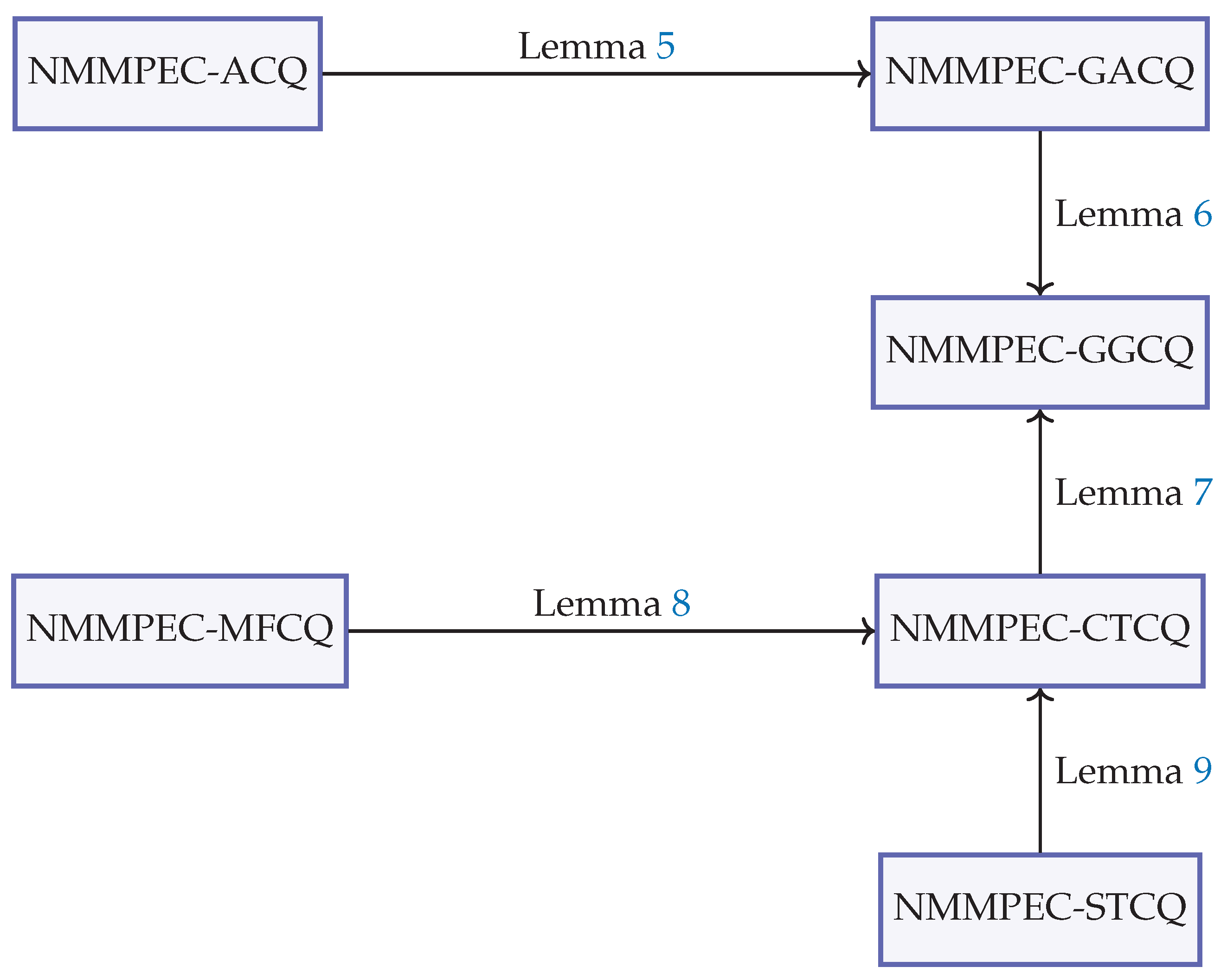
The results derived in this section are summarized in the following theorem.

Theorem 3.

Let $a^{*}\in \mathcal{S}$ be a Pareto efficient solution of (NMMPEC) and let ${\mathcal{R}}_{00}=\mathcal{F}$. If any of the constraint qualifications as defined in Definitions 11-15 is satisfied at $a^{*}$, then (NMMPEC-GGCQ) holds at $a^{*}$, and there exist real numbers ${\alpha }_j$$(j\in \mathcal{I})$, ${\sigma }_j^{\mathcal{W}}$$(j\in {\mathcal{I}}^{\mathcal{W}})$, ${\sigma }_j^{\mathcal{V}}$$(j\in {\mathcal{I}}^{\mathcal{V}})$, ${\sigma }_j^{\mathcal{C}}$$(j\in \mathcal{T})$, ${\sigma }_j^{\mathcal{D}}$$(j\in \mathcal{T})$ which satisfy equation (7) and equation (8).

Remark 7.

Theorem 3 generalizes Theorem 4.1 of Maeda [27] from multiobjective programming problems to (NMMPEC) and extends it from Euclidean spaces to the setting of Hadamard manifolds.

The results that are established in the present section can be summarized and conveniently visualized from Figure 1.

In the following numerical example, we consider the Hadamard manifold consisting of the set of all symmetric positive definite matrices, where the corresponding Riemannian metric is given by the Hessian of the standard logarithmic barrier $B\left(\mathcal{X}\right)=-lndet\left(\mathcal{X}\right)$, where $\mathcal{X}$ is any symmetric positive definite matrix (see, for instance, [3,30]). Such manifolds widely appear in medical image processing, for instance, in modeling of the covariance matrix of the Brownian motion of water in diffusion tensor imaging (see, for instance, [32]).

Example 2.

Let ${\mathcal{M}}^2$ denote the set of all symmetric matrices of order $2\times 2$. For any matrix $\mathcal{B}$, the notation $Tr\left(\mathcal{B}\right)$ denotes the trace of the matrix $\mathcal{B}$. Consider the set ${\mathcal{P}}_{+}^2\subset {\mathcal{M}}^2$, consisting of every symmetric positive definite matrix of order $2\times 2$. Let $\mathcal{A}\in {\mathcal{P}}_{+}^2$. The set ${\mathcal{P}}_{+}^2$ is a Hadamard manifold that is endowed with the following metric (see, for instance, [13,26]):

$${\langle {\mathcal{B}}_1,{\mathcal{B}}_2\rangle }_{\mathcal{A}}:=Tr\left({\mathcal{B}}_2{\mathcal{A}}^{-1}{\mathcal{B}}_1{\mathcal{A}}^{-1}\right),$$

for any arbitrary ${\mathcal{B}}_1$, ${\mathcal{B}}_2\in T_{\mathcal{A}}{\mathcal{P}}_{+}^2={\mathcal{M}}^2$. Consider any arbitrary pair of elements $\mathcal{X},\mathcal{D}\in {\mathcal{P}}_{+}^2$ and $\mathcal{B}\in T_{\mathcal{X}}{\mathcal{P}}_{+}^2$.

Then, the corresponding exponential function ${exp}_{\mathcal{X}}\left(\mathcal{B}\right):T_{\mathcal{X}}{\mathcal{P}}_{+}^2\to {\mathcal{P}}_{+}^2$ is given by

$${exp}_{\mathcal{X}}\left(\mathcal{B}\right)={\mathcal{X}}^{{\displaystyle \frac{1}{2}}}Exp\left({\mathcal{X}}^{-{\displaystyle \frac{1}{2}}}\mathcal{B}{\mathcal{X}}^{-{\displaystyle \frac{1}{2}}}\right){\mathcal{X}}^{{\displaystyle \frac{1}{2}}},$$

where the symbol Exp stands for matrix exponential (see, for instance, [26]). Further, the inverse exponential function ${exp}_{\mathcal{X}}^{-1}:{\mathcal{P}}_{+}^2\to T_{\mathcal{X}}{\mathcal{P}}_{+}^2$ is given by

$${exp}_{\mathcal{X}}^{-1}\left(\mathcal{D}\right)={\mathcal{X}}^{{\displaystyle \frac{1}{2}}}Log\left({\mathcal{X}}^{-{\displaystyle \frac{1}{2}}}\mathcal{D}{\mathcal{X}}^{-{\displaystyle \frac{1}{2}}}\right){\mathcal{X}}^{{\displaystyle \frac{1}{2}}},$$

where the symbol Log is the usual logarithm on $P_{+}^2$ (see, for instance, [26]). For any real-valued function $F:{\mathcal{P}}_{+}^2\to \mathbb{R}$ the Riemannian gradient is given by:

$$grad\left(F\left(\mathcal{X}\right)\right)=\mathcal{X}{F}^{\prime }\left(\mathcal{X}\right)\mathcal{X},$$

for any $\mathcal{X}\in {\mathcal{P}}_2^{+}$, where $F^{\prime }\left(\mathcal{X}\right)$ denotes the Euclidean gradient of the function F at $\mathcal{X}$ (see, for instance, [13]).

Consider the following problem (P), which is a (NMSIPMC):

$$\begin{array}{cc}\hfill \left(P\right)\mathit{Min}\mathcal{F}\left(\mathcal{X}\right)=({\mathcal{F}}_1\left(\mathcal{X}\right),& {\mathcal{F}}_2\left(\mathcal{X}\right)):=(-3\log c_1-3\log c_4,-5-log{c}_1-log{c}_4),\hfill \\ \hfill \mathit{subject}\mathit{to}& {\mathcal{C}}_1\left(\mathcal{X}\right):=1-\left|c_4\right|\ge 0,\hfill \\ \hfill & {\mathcal{D}}_1\left(\mathcal{X}\right):=1-\left|c_1\right|\ge 0,\hfill \\ \hfill & {\mathcal{C}}_1\left(\mathcal{X}\right){\mathcal{D}}_1\left(\mathcal{X}\right):=(1-|c_4\left|\right)(1-|c_1\left|\right)=0,\hfill \end{array}$$

where ${\mathcal{F}}_i:{\mathcal{P}}_2^{+}\to \mathbb{R}$$(i=1,2)$ and ${\mathcal{C}}_1,{\mathcal{D}}_1:{\mathcal{P}}_2^{+}\to \mathbb{R}$ are locally Lipschitz functions and $\mathcal{X}=\left[\begin{array}{cc}{c}_1& c_2\\ c_2& c_4\end{array}\right]\in {\mathcal{P}}_2^{+}$.We use the symbol $\mathcal{S}$ to signify the set consisting of every feasible element of (P). By simple calculations, we obtain the following:

$$\begin{array}{c}\hfill \mathcal{S}=\left\{\left[\begin{array}{cc}{c}_1& 0\\ 0& c_4\end{array}\right]:c_4=1,0<c_1\le 1,\mathrm{or}{c}_1=1,0<c_4\le 1\right\}.\end{array}$$

We choose the feasible element

$${\mathcal{X}}^{*}=\left[\begin{array}{ccc}1& & 0\\ 0& & 1\end{array}\right]\in \mathcal{S}.$$

It can be verified that ${\mathcal{X}}^{*}$ is a Pareto efficient solution of (NMSIPMC). Then, we can obtain the following:

$$\begin{array}{cccc}\hfill {\partial }^c{\mathcal{F}}_1\left({\mathcal{X}}^{*}\right)& =\left\{\left[\begin{array}{ccc}-3& & 0\\ 0& & -3\end{array}\right]\right\},\hfill & \hfill & {\partial }^c{\mathcal{F}}_2\left({\mathcal{X}}^{*}\right)=\left\{\left[\begin{array}{ccc}-1& & 0\\ 0& & -1\end{array}\right]\right\},\hfill \\ \hfill {\partial }^c{\mathcal{C}}_1\left({\mathcal{X}}^{*}\right)& =\left\{\left[\begin{array}{ccc}0& & 0\\ 0& & 1\end{array}\right]\right\},\hfill & \hfill & {\partial }^c{\mathcal{D}}_1\left({\mathcal{X}}^{*}\right)=\left\{\left[\begin{array}{ccc}1& & 0\\ 0& & 0\end{array}\right]\right\}.\hfill \end{array}$$

By simple calculations, we may obtain the following:

$$\begin{array}{cc}\hfill {\mathcal{C}}^{Lin}(\mathcal{L},{\mathcal{X}}^{*})& =\left\{\left[\begin{array}{cc}0& c_2\\ c_2& 0\end{array}\right]:c_2\in \mathbb{R}\right\},\hfill \\ \hfill {\mathcal{C}}^{Tan}(\mathcal{L},{\mathcal{X}}^{*})& =\left\{\left[\begin{array}{cc}{c}_1& c_2\\ c_3& c_4\end{array}\right]:c_1,c_2,c_3,c_4=0\right\},\hfill \end{array}$$

Consequently, it can be verified that (NMMPEC-ACQ) is not satisfied at ${\mathcal{X}}^{*}$. Let us now choose real numbers ${\sigma }_1^{\mathcal{F}}={\displaystyle \frac{1}{2}}$, ${\sigma }_2^{\mathcal{F}}={\displaystyle \frac{1}{2}}$, ${\sigma }_1^{\mathcal{C}}=2$, ${\sigma }_1^{\mathcal{D}}=2$. Then, we have

$$\begin{array}{cc}\hfill {\sigma }_1^{\mathcal{F}}\left[\begin{array}{ccc}-3& & 0\\ 0& & -3\end{array}\right]+{\sigma }_2^{\mathcal{F}}\left[\begin{array}{ccc}-1& & 0\\ 0& & -1\end{array}\right]+& {\sigma }_1^{\mathcal{C}}\left[\begin{array}{ccc}0& & 0\\ 0& & 1\end{array}\right]+{\sigma }_1^{\mathcal{D}}\left[\begin{array}{ccc}1& & 0\\ 0& & 0\end{array}\right]=\left[\begin{array}{ccc}0& & 0\\ 0& & 0\end{array}\right].\hfill \end{array}$$

As a result, we infer the fact that although (NMMPEC-ACQ) fails to be satisfied at ${\mathcal{X}}^{*}$, the conclusions of Theorem 3 may still be satisfied. Consequently, this numerical example illustrates that satisfaction of (NMMPEC-ACQ) is merely a sufficient, but not a necessary condition for satisfaction of KKT conditions at a Pareto efficient solution of (NMMPEC).

5. Conclusions and Future Directions

In this article, we have investigated a class of (NMMPEC) in the setting of Hadamard manifolds. (NMMPEC-GGCQ) for (NMMPEC) has been introduced in the framework of Hadamard manifolds. We have established the necessary criteria of Pareto efficiency for (NMMPEC) using (NMMPEC-GGCQ). Subsequently, we have introduced several (NMMPEC)-tailored constraint qualifications, for instance, (NMMPEC-ACQ), (NMMPEC-GACQ), (NMMPEC-CTCQ), (NMMPEC-STCQ), (NMMPEC-MFCQ) in the Hadamard manifold setting. We have established several interesting interrelations between these constraint qualifications. Moreover, we have established that these constraint qualifications are sufficient conditions for (NMMPEC-GGCQ). We have furnished some non-trivial examples to justify the importance of the deduced results.

The results derived in this article extend the corresponding results established by Maeda [27] for (NMMPEC) in Hadamard manifold setting. Furthermore, the results derived in this article extend the corresponding notions of constraint qualifications studied by Flegel and Kanzow in [15,16] on the setting of more general space, that is, Hadamard manifolds, and generalize them for a more general category of optimization problems, that is, (NMMPEC). Moreover, the optimality criteria derived in the present article extend the corresponding results established by Treanţă et al. [37], for a more general category of optimization problems, namely, (NMMPEC).

The results established in the present article leave numerous options for future research work. For instance, it would be an interesting research problem to investigate constraint qualifications for nonsmooth multiobjective programming problems with switching constraints on Hadamard manifolds via convexificators. This would be our future course of study.

References

- Ahmadian, S.; Tang, X.; Malki, H.A.; Han, Z. Modelling cyber attacks on electricity market using mathematical programming with equilibrium constraints. IEEE Access 2019, 7, 27376–27388. [Google Scholar] [CrossRef]
- Ardali, A.A.; Movahedian, N.; Nobakhtian, S. Optimality conditions for nonsmooth mathematical programs with equilibrium constraints using convexificators. Optimization 2014, 65, 67–85. [Google Scholar] [CrossRef]
- Bacák, M.; Bergmann, R.; Steidl, G.; Weinmann, A. A second order nonsmooth variational model for restoring manifold-valued images. SIAM J. Sci. Comput. 2016, 38, A567–A597. [Google Scholar] [CrossRef]
- Barani, A. Generalized monotonicity and convexity for locally Lipschitz functions on Hadamard manifolds. Differ. Geom. Dyn. Syst. 2013, 15, 26–37. [Google Scholar]
- Belkin, M.; Niyogi, P. Semi-supervised learning on Riemannian manifolds. Mach. Learn. 2004, 56, 209–239. [Google Scholar] [CrossRef]
- Bergmann, R.; Herzog, R. Intrinsic formulation of KKT conditions and constraint qualifications on smooth manifolds. SIAM J. Optim. 2019, 29, 2423–2444. [Google Scholar] [CrossRef]
- Boumal, N.; Mishra, B.; Absil, P.-A.; Sepulchre, R. Manopt: A MATLAB toolbox for optimization on manifolds. J. Mach. Learn. Res. 2014, 15, 1455–1459. [Google Scholar]
- Britz, W.; Ferris, M.; Kuhn, A. Modeling water allocating institutions based on multiple optimization problems with equilibrium constraints. Environ. Model. Softw. 2013, 46, 196–207. [Google Scholar] [CrossRef]
- Chen, S. Existence results for vector variational inequality problems on Hadamard manifolds. Optim. Lett. 2020, 14, 2395–2411. [Google Scholar] [CrossRef]
- Chen, Y.; Florian, M. The nonlinear bilevel programming problem: Formulations, regularity and optimality conditions. Optimization 1995, 32, 193–209. [Google Scholar] [CrossRef]
- Colao, V.; López, G.; Marino, G.; Martín-Márquez, V. Equilibrium problems in Hadamard manifolds. J. Math. Anal. Appl. 2012, 388, 61–77. [Google Scholar] [CrossRef]
- Ferreira, O.P. Proximal subgradient and a characterization of Lipschitz function on Riemannian manifolds. J. Math. Anal. Appl. 2006, 313, 587–597. [Google Scholar] [CrossRef]
- Ferreira, O.P.; Louzeiro, M.S.; Prudente, L. Gradient method for optimization on Riemannian manifolds with lower bounded curvature. SIAM J. Optim. 2019, 29, 2517–2541. [Google Scholar] [CrossRef]
- Fletcher, P.T.; Moeller, J.; Phillips, J.M.; Venkatasubramanian, S. Horoball hulls and extents in positive definite space. In Algorithms and Data Structures; Springer: Berlin/Heidelberg, Germany, 2011; pp. 386–398. [Google Scholar]
- Flegel, M.L.; Kanzow, C. Abadie-type constraint qualification for mathematical programs with equilibrium constraints. J. Optim. Theory Appl. 2005, 124, 595–614. [Google Scholar] [CrossRef]
- Flegel, M.L.; Kanzow, C. On the Guignard constraint qualification for mathematical programs with equilibrium constraints. Optimization 2005, 54, 517–534. [Google Scholar] [CrossRef]
- Ghosh, A.; Upadhyay, B.B.; Stancu-Minasian, I.M. Constraint qualifications for multiobjective programming problems on Hadamard manifolds. Aust. J. Math. Anal. Appl. 2023, 20, 1–17. [Google Scholar]
- Ghosh, A.; Upadhyay, B.B.; Stancu-Minasian, I.M. Pareto efficiency criteria and duality for multiobjective fractional programming problems with equilibrium constraints on Hadamard manifolds. Mathematics 2023, 11, 3649. [Google Scholar] [CrossRef]
- Grohs, P.; Hosseini, S. ϵ-subgradient algorithms for locally Lipschitz functions on Riemannian manifolds. Adv. Comput. Math. 2016, 42, 333–360. [Google Scholar] [CrossRef]
- Harker, P.T.; Pang, J.S. Existence of optimal solutions to mathematical programs with equilibrium constraints. Oper. Res. Lett. 1988, 7, 61–64. [Google Scholar] [CrossRef]
- Hejazi, M.A. On constraint qualifications for multiobjective programming problems with equilibrium constraints. J. Math. Ext. 2018, 12, 25–39. [Google Scholar]
- Hosseini, S.; Huang, W.; Yousefpour, R. Line search algorithms for locally Lipschitz functions on Riemannian manifolds. SIAM J. Optim. 2018, 28, 596–619. [Google Scholar] [CrossRef]
- Hosseini, S.; Pouryayevali, M.R. Generalized gradients and characterization of epi-Lipschitz sets in Riemannian manifolds. Nonlinear Anal. 2011, 74, 3884–3895. [Google Scholar] [CrossRef]
- Karkhaneei, M.M.; Mahdavi-Amiri, N. Nonconvex weak sharp minima on Riemannian manifolds. J. Optim. Theory Appl. 2019, 183, 85–104. [Google Scholar] [CrossRef]
- Li, X.B.; Zhou, L.W.; Huang, N.J. Gap functions and descent methods for equilibrium problems on Hadamard manifolds. J. Nonlinear Convex Anal. 2016, 17, 807–826. [Google Scholar]
- Lim, Y.; Hiai, F.; Lawson, J. Nonhomogeneous Karcher equations with vector fields on positive definite matrices. Eur. J. Math. 2021, 7, 1291–1328. [Google Scholar] [CrossRef]
- Maeda, T. Constraint qualifications in multiobjective optimization problems: Differentiable case. J. Optim. Theory Appl. 1994, 80, 483–500. [Google Scholar] [CrossRef]
- Mishra, S.K.; Upadhyay, B.B. Pseudolinear Functions and Optimization; Chapman and Hall/CRC: London, UK, 2019. [Google Scholar]
- Papa Quiroz, E.A.; Quispe, E.M.; Oliveira, P.R. Steepest descent method with a generalized Armijo search for quasiconvex functions on Riemannian manifolds. J. Math. Anal. Appl. 2009, 341, 467–477. [Google Scholar] [CrossRef]
- Papa Quiroz, E.A.; Oliveira, P.R. Full convergence of the proximal point method for quasiconvex functions on Hadamard manifolds. ESAIM Control Optim. Calc. Var. 2012, 18, 483–500. [Google Scholar] [CrossRef]
- Papa Quiroz, E.A.; Oliveira, P.R. Proximal point methods for quasiconvex and convex functions with Bregman distances on Hadamard manifolds. J. Convex Anal. 2009, 16, 49–69. [Google Scholar]
- Pennec, X. Manifold-valued image processing with SPD matrices. In Riemannian Geometric Statistics in Medical Image Analysis; Elsevier: Amsterdam, The Netherlands, 2020; pp. 75–134. [Google Scholar]
- Ralph, D. Mathematical programs with complementarity constraints in traffic and telecommunications networks. Philos. Trans. R. Soc. A 2008, 366, 1973–1987. [Google Scholar] [CrossRef]
- Rapcsák, T. Smooth Nonlinear Optimization in ; Springer: Berlin, Germany, 2013. [Google Scholar]
- Stein, O. On constraint qualifications in nonsmooth optimization. J. Optim. Theory Appl. 2004, 121, 647–671. [Google Scholar] [CrossRef]
- Singh, K.V.K.; Mishra, S.K. On multiobjective mathematical programming problems with equilibrium constraints. Appl. Math. Inf. Sci. Lett. 2019, 7, 17–25. [Google Scholar] [CrossRef]
- Treanţă, S.; Upadhyay, B.B.; Ghosh, A.; Nonlaopon, K. Optimality conditions for multiobjective mathematical programming problems with equilibrium constraints on Hadamard manifolds. Mathematics 2022, 10, 3516. [Google Scholar] [CrossRef]
- Tung, L.T.; Tam, D.H. Optimality conditions and duality for multiobjective semi-infinite programming on Hadamard manifolds. Bull. Iran. Math. Soc. 2022, 48, 2191–2219. [Google Scholar] [CrossRef]
- Udrişte, C. Convex Functions and Optimization Methods on Riemannian Manifolds; Springer: Berlin, Germany, 2013. [Google Scholar]
- Upadhyay, B.B.; Ghosh, A. Optimality conditions and duality for multiobjective semi-infinite optimization problems with switching constraints on Hadamard manifolds. Positivity 2024, 28, 1–26. [Google Scholar] [CrossRef]
- Upadhyay, B.B.; Ghosh, A. On constraint qualifications for mathematical programming problems with vanishing constraints on Hadamard manifolds. J. Optim. Theory Appl. 2023, 200, 794–819. [Google Scholar] [CrossRef]
- Upadhyay, B.B.; Ghosh, A.; Kanzi, N. Constraint qualifications and optimality conditions for nonsmooth multiobjective mathematical programming problems with vanishing constraints on Hadamard manifolds via convexificators. J. Math. Anal. Appl. 2025, 542, 128873. [Google Scholar] [CrossRef]
- Upadhyay, B.B.; Ghosh, A.; Kanzi, N.; Soroush, H. Constraint qualifications for nonsmooth multiobjective programming problems with switching constraints on Hadamard manifolds. Bull. Malays. Math. Sci. Soc. 2024, 47, 103. [Google Scholar] [CrossRef]
- Upadhyay, B.B.; Ghosh, A.; Mishra, P.; Treanţă, S. Optimality conditions and duality for multiobjective semi-infinite programming problems on Hadamard manifolds using generalized geodesic convexity. RAIRO Oper. Res. 2022, 56, 2037–2065. [Google Scholar] [CrossRef]
- Upadhyay, B.B.; Ghosh, A.; Treanţă, S.; Yao, J.-C. Constraint qualifications and optimality conditions for multiobjective mathematical programming problems with vanishing constraints on Hadamard manifolds. Mathematics 2024, 12, 347. [Google Scholar] [CrossRef]
- Upadhyay, B.B.; Ghosh, A.; Treanţă, S. Efficiency conditions and duality for multiobjective semi-infinite programming problems on Hadamard manifolds. J. Glob. Optim. 2024, 89, 723–744. [Google Scholar] [CrossRef]
- Upadhyay, B.B.; Ghosh, A.; Stancu-Minasian, I.M. Second-order optimality conditions and duality for multiobjective semi-infinite programming problems on Hadamard manifolds. Asia-Pac. J. Oper. Res. 2023, 41, 2350019. [Google Scholar] [CrossRef]
- Upadhyay, B.B.; Ghosh, A.; Treanţă, S. Optimality conditions and duality for nonsmooth multiobjective semi-infinite programming problems with vanishing constraints on Hadamard manifolds. J. Math. Anal. Appl. 2024, 531, 127785. [Google Scholar] [CrossRef]
- Upadhyay, B.B.; Ghosh, A.; Treanţă, S. Constraint qualifications and optimality criteria for nonsmooth multiobjective programming problems on Hadamard manifolds. J. Optim. Theory Appl. 2024, 200, 794–819. [Google Scholar] [CrossRef]
- Upadhyay, B.B.; Ghosh, A.; Treanţă, S. Optimality conditions and duality for nonsmooth multiobjective semi-infinite programming problems on Hadamard manifolds. Bull. Iran. Math. Soc. 2023, 49, 1–36. [Google Scholar] [CrossRef]
- Ye, J.J. Necessary and sufficient optimality conditions for mathematical programs with equilibrium constraints. J. Math. Anal. Appl. 2005, 307, 350–369. [Google Scholar] [CrossRef]
- Zhang, P.; Zhang, J.; Lin, G.H.; Yang, X. Constraint qualifications and proper Pareto optimality conditions for multiobjective problems with equilibrium constraints. J. Optim. Theory Appl. 2018, 176, 763–782. [Google Scholar] [CrossRef]
Figure 1.
Interralations among the constraint qualifications for (NMMPEC)
Disclaimer/Publisher’s Note: The statements, opinions and data contained in all publications are solely those of the individual author(s) and contributor(s) and not of MDPI and/or the editor(s). MDPI and/or the editor(s) disclaim responsibility for any injury to people or property resulting from any ideas, methods, instructions or products referred to in the content. |
© 2025 by the authors. Licensee MDPI, Basel, Switzerland. This article is an open access article distributed under the terms and conditions of the Creative Commons Attribution (CC BY) license (http://creativecommons.org/licenses/by/4.0/).
Copyright: This open access article is published under a Creative Commons CC BY 4.0 license, which permit the free download, distribution, and reuse, provided that the author and preprint are cited in any reuse.