
Submitted:
31 October 2025
Posted:
03 November 2025
You are already at the latest version
Abstract
Conventional vibration-based condition monitoring of wind turbine drivetrains typically relies on feature extraction guided by expert experience and prior knowledge. However, the effectiveness of this approach is often limited when such knowledge is insufficient or when fault features are obscured by high levels of ambient noise. To address these challenges, this paper proposes an innovative data-driven framework that integrates intelligent feature extraction with a deep learning architecture. In the proposed approach, bearing vibration signals are converted into the frequency domain, and the frequency spectrum is divided into multiple frequency bands. The relative importance of each band is evaluated and ranked using XGBoost, enabling the selection of the most informative features and significant dimensionality reduction. A hybrid CNN–Transformer model is then employed to combine local feature extraction with global attention mechanisms for accurate fault classification. Experimental evaluations using two open-source datasets demonstrate that the proposed framework achieves high classification accuracy and rapid convergence, offering a robust and computationally efficient solution for wind turbine drivetrain fault diagnosis.
Keywords:
wind turbine
; fault diagnosis
; XGBoost
; feature selection
; deep learning
1. Introduction
Wind turbines are key assets in modern renewable energy systems, particularly in coastal and offshore environments where wind resources are abundant [1]. However, their drivetrains, comprising gearboxes, generators, and other rotating elements, operate under highly dynamic loads and harsh marine conditions that accelerate wear and promote fault development [2]. Faults in wind turbine drivetrains are generally grouped into three categories. a) Electrical faults, including generator winding failures and insulation breakdowns. b) Mechanical faults, which are the most frequent in practice and typically arise in gearboxes, bearings, and shafts. c) Environmental and control-related faults, such as those caused by wet and corrosive offshore environments or control system malfunctions [3].
Among these, mechanical faults in drivetrain rotating components are especially critical because they often escalate into severe damage and are associated with long downtime and high maintenance costs if not identified at an early stage [4]. As these faults typically manifest through changes in dynamic behaviour, they can be detected most effectively through vibration analysis [5]. Therefore, vibration signals remain one of the most informative indicators of such problems due to their sensitivity to structural and dynamic changes [6].
Traditional vibration-based condition monitoring methods typically rely on signal processing techniques, and the main purpose of signal processing is to cancel the noise contained in the vibration signals and then extract the fault-related features based on prior knowledge. For example, in [7], authors reduced the noise in the vibration signal by the approach of combining variational mode decomposition (VMD), correlation analysis, and wavelet-threshold de-noising; In [8], the proposed method extracts instantaneous frequency features from vibration signals to detect different fault types of rolling bearings under variable speed conditions. Usually, such signal processing workflows are not only laborious and time-consuming but also heavily reliant on the operator’s expertise and experience.
In recent years, artificial intelligence (AI) techniques have been increasingly integrated into machine condition monitoring. Compared with traditional vibration-based condition monitoring methods that rely on professional knowledge on feature extraction and fault diagnosis, AI-assisted approaches can automatically learn patterns or features from vibration signals and distinguish between different types of faults [9]. In past years, a variety of machine learning algorithms, such as Support Vector Machines (SVMs), Logistic Regression, and K-Nearest Neighbours (KNNs) have been widely used for fault detection based on extracted features from vibration signals [10]. Taking decision Tree as an example, it has been one of the most common and widely used traditional machine learning models used since 1980s[11]. In [12], the authors apply decision tree algorithms for wind turbine structure condition monitoring by leveraging their fast learning, ease of interpretation, ability to support clear fault tracing, and strong performance when both error rate and training speed are considered. A further example of decision tree’s application is presented in [13], where it is used for planetary gearbox condition monitoring, which highlights its capability for motor-driven system condition monitoring using statistical features. Recent research also demonstrates the effectiveness of decision trees for lightweight fault classification tasks implemented on edge devices [14], where a fine decision tree classifier was deployed on a microcontroller for real-time fault detection in rotating machinery using extracted features. However, despite popularity and their advantages, decision tree-assisted condition monitoring methods have some obvious drawbacks. For example, decision trees tend to overfit easily during training, resulting in poor generalization [15], and this is especially problematic in the cases where noisy data is used, because these kinds of models are excessively sensitive to slight changes in training sets [16]. To address these weaknesses, Extreme Gradient Boosting (XGBoost) has been proposed as an enhanced tree-based ensemble learning method. In [17], the XGBoost model is used in conjunction with the Mel Frequency Spectral Coefficient features extracted from vibration data for the classification of roller bearing faults. And in [18] , the accuracy of the XGBoost model was compared with other classic machine learning models and showed the highest accuracy for bearing faults.
In addition to performance, interpretability is another key advantage that decision tree-based models have in condition monitoring applications [19]. These tree-based models offer transparent and rule-based reasoning by constructing explicit paths from input features to output targets [20]. This makes them particularly useful in applications where interpretability and fault traceability are important. The most common scenario where the interpretability of tree-based models is feature selection, where the importance of different features will be calculated and ranked, allowing only the features of high importance to be used for further analysis. In [21], authors applied XGBoost with feature importance ranking to reduce redundant sensor data and improve fault classification performance. And in [22], authors used XGBoost model to rank the importance of more than 300 statistical features extracted from vibration and cutting force signal and selected only 14 features in the training stage significantly improving the training efficiency and prediction accuracy. However, tree-based models including XGBoost still have a key drawback: They rely heavily on artificially designed indicators, such as statistical metrics. These indicators cannot guarantee that they can effectively distinguish the health status and fault type of the machine.
More recently, deep learning (DL) models have been increasingly used attributed to their ability to learn complex patterns from raw or processed vibration signals. For example, Convolutional Neural Networks (CNNs) are effective in capturing spatial patterns across different vibration signal domains [23]; Recurrent Neural Networks (RNNs) are specialized in sequential data such as time-series vibration signals [24]. Transformers, with their multi-head attention mechanisms, have demonstrated strong performance in handling complex signals and capturing dependencies from large data segments [25]. To overcome the reliance on artificially designed features, recent studies have increasingly turned to DL approaches that are capable of identifying meaningful patterns directly from complex or noisy data with high generalizability [26]. Among them, CNNs have demonstrated strong performance in extracting meaningful patterns from raw signals. 1-Dimensional (1D) CNNs usually operate directly on raw time-series data. For example, in [27], a 1D CNN was proposed to process raw vibration and phase current signals for bearing fault classification. In [28], a 1D CNN was used as the feature extractor for vibration signals in a Zero-Shot Learning (ZSL) framework, where Semantic Feature Space mapping was adopted for intelligent fault detection of unseen faults. In contrast, 2D CNNs are usually applied to transformed representations of raw signals, such as frequency maps, time-frequency maps, or images generated by self-defined approaches from raw signals. In [29], a 2D CNN was employed to extract grayscale images from enhanced frequency maps of vibration signals, achieving high classification accuracy using undersampled signals. On the other hand, the Transformer model, which was originally proposed in [30], has also demonstrated high performance to capture long-range dependencies through self-attention mechanisms. In [31], a transformer-based model was proposed to predict the remaining useful life of the bearing lubricant using the frequency domain of the vibration signal. In [32], a transformer model was used for rolling bearing fault diagnosis, using time-frequency representations of wavelet transforms to capture non-stationary signal patterns and long-range dependencies.
By combining the local feature extraction capability of CNNs with the global dependency modelling of transformer-based architectures, recent studies have proposed hybrid models, CNN-Transformer models. In [33], a CNN-Transformer multitask model was proposed for simultaneously performing both bearing fault diagnosis and severity assessment, utilizing the local feature extraction ability of CNNs and global sequence modelling ability of Transformer to improve DL model robustness. In [34], authors developed a CNN-Transformer model for rotating machinery fault classification under varying operational conditions. Similarly, CNNs were used for multi-scale feature extraction, and Transformer blocks were introduced to link the relationship between fault patterns and fault types.
While DL models and their combined architectures have achieved popularity in vibration-based condition monitoring, they also present limitations. To extract meaningful patterns from complex and noisy raw vibration signal or its representations, these models are usually high in complexity, involving large number of parameters and layers, that makes them difficult to design, train, and fine-tune [35]. In addition, the scarcity of useful data and their reliance on large training data and computationally intensive operations can pose significant challenges in terms of resource availability, resource consumption, and training time. These factors can limit their practical deployment, especially in real-time or resources-constrained platforms such as edge devices [36]. Therefore, it is necessary to find a practical way to utilise the powerful capabilities of DL models while keeping them structurally simple and computationally efficient, as well as enhancing their interpretability. This motivates the research reported below.
The main contribution of this paper is the development of a novel vibration-based fault classification framework, which integrates interpretable spectral analysis and XGBoost-based frequency band selection, following with a CNN-Transformer hybrid model for efficient and accurate fault diagnosis.
The effectiveness of the proposed method is validated on two widely accepted open-source datasets, the CWRU bearing dataset and the BJTU planetary gearbox dataset. Demonstrating its robustness across different fault types and mechanical systems. Furthermore, the proposed frequency-band selection strategy significantly reduces the input feature dimensionality for deep-learning model training, thereby improving computational efficiency without compromising classification performance.
The remainder of this paper is organized as follows: Section 2 depicts the proposed fault classification framework, covering the frequency band selection using XGBoost and the CNN-Transformer classifier; Section 3 describes two open-access datasets used in this study. Section 4 demonstrates and discusses the training results and performance analysis of proposed method on both datasets. Section 5 concludes the study and outlines directions for future work.
2. Methodology
This section presents the proposed vibration-based fault classification framework, as depicted in Figure 1.
As shown in Figure 1, the proposed framework integrates XGBoost-assisted frequency band selection with a DL model to achieve high classification accuracy while maintaining computational efficiency. This method is designed to leverage the interpretability of tree-based models and the powerful pattern recognition capability of hybrid DL models. In the DL architecture, both the CNN and Transformer blocks can be stacked to form multi-layer structures, where the depth of each component is determined based on the complexity of the vibration signals being analysed and the concrete requirements of feature extraction. The proposed method consists of three main stages: 1) Raw signal preprocessing, vibration signals are divided into multiple segments and transformed into frequency spectra. 2) XGBoost-assisted frequency band selection, where the frequency spectrum of the signal will be divided into several frequency bands, and XGBoost is then employed to evaluate and rank the importance of each band. Only those bands of high importance will be retained and concatenated. 3) DL-based fault classification, i.e., the prepared frequency features will be used as input to a CNN-Transformer model, for performing fault classification.
2.1. Raw Signal Segmentation and Preprocessing
In the first stage of the proposed method, the raw vibration signal is segmented with the aid of a fixed-length window to facilitate frequency-domain transformation. The window will slide along the signal and the stride of window movement at each time can be adjusted depending on different applications. Normally, using a smaller stride increases the total number of samples that can be extracted from the raw signal, but it also introduces high computational demand since more data is used for training. In this study, the stride is initially set equal to the window length to create non-overlapping segments, and it can be adjusted depending on the sampling rate and data length of the signals in the dataset. The non-overlapping setup avoids duplicate content between samples and reduces computational cost. The data in a segment can be expressed by the following equation:
Where x is the full vibration signal in one-dimension array, stands for the n-th segment, represents the window length, S denotes the stride between two consecutive segments, and is the segment index.
Each is then transformed into the frequency domain using the Discrete Fourier Transform (DFT), which is implemented efficiently using the Fast Fourier Transform (FFT) algorithm. The DFT of the n-th segment is computed as [37]:
Where represents the complex DFT coefficient at Frequency bin f, is the k-th data sample within segment .
To convert the complex output into real-valued features, the magnitude spectrum is computed as:
Where and are the real and imaginary parts of , respectively.
This stage transforms the segmented sets of raw vibration signals into a frequency domain representation that will be used as input for the feature selection stage described in the next stage.
2.2. XGBoost-Assisted Frequency Band Selection
Following the transformation of each segmented vibration signal into the frequency spectrum, the resulting magnitude spectrums are typically high-dimensional, consisting of magnitude values across frequencies. However, these frequency components in the spectrum never contribute equally to fault-classification tasks. To identify the most informative frequency components for classification, a feature selection strategy based on the XGBoost algorithm is proposed.
To simplify the calculation, the one-dimensional frequency spectrum is divided into multiple parts first, referred to as frequency bands. Each frequency band contains the same number of consecutive frequency components. To organize the frequency spectrum into frequency bands, the following equations are used:
Where is the total number of data in the frequency spectrum of each signal segment. M denotes the number of frequency components included in each band. indicates the total number of frequency bands created. is the stride used when sliding window along the spectrum.
The Equation (5) is used for two purposes: when the , it gives the maximum number of non-overlapping bands from the spectrum. When , it indicates the total number of band importance scores that will be computed during the feature selection stage.
The XGBoost is a high-performance ensemble learning algorithm based on gradient boosting, which constructs a strong classifier by sequentially combining multiple weak learner (decision trees). Each tree is trained to correct the residual errors made by the previous trees, and the entire process minimizes a regularized objective function to ensure generalization and prevent over-fitting. The basic framework of XGBoost algorithm can be expressed by the following equation [38]:
Where denotes the predicted output for the i-th of sample x, the is the function space which represents all regression functions. is an individual weak learner. K is the number of weak learners added sequentially.
To formalize the training objective, the total loss function minimized by the XGBoost algorithm combines both the training loss and a regularization term that penalizes model complexity. This is defined as:
Where represents the total loss, is the loss between the actual value and the predicted value , and indicates the regularization term for each weak learner, which quantifies the complexity of the model.
During training, the at the t-th iteration can be expressed as:
Where is the prediction from the last tree, and is the tree at current step t.
For multi-class classification tasks, the categorical cross-entropy loss, also know as the multi-class logarithmic loss is used to quantify the classification error during XGBoost model training, it is defined as:
Where represents the total number of training samples, C denotes the number of classes, is a binary indicator (1 if sample i belongs to class k, otherwise 0). And is the predicted probability of i belongs to class k which is calculated using Softmax function in Equation (10) where denotes the raw score output by the model for class c.
To identify those high-importance frequency bands in the spectrum, we leverage the gain-based feature importance measure from the XGBoost framework. In this study, each input sample consists of the magnitudes of frequency components. During training, XGBoost evaluates potential splits in decision trees using the expected improvement in the loss function. This improvement is referred to as "gain". The gain for a split at a decision node is calculated as:
Where and are the sums of the first-order gradients for the left and right leaves, and are the sums of second-order gradients, is the regularization term on leaf weights, and represents the complexity penalty for adding a new leaf.
By summing the gain across all nodes and all trees where a frequency component is used for splitting, XGBoost computes a total importance score for each frequency component. However, rather than focus on individual components, this study emphasizes the identification of the most important frequency bands for fault classification. To achieve this, importance scores are aggregated within fixed-width frequency bands. This approach reflects the fact that fault-induced spectral patterns often span across multiple adjacent frequency components, making it more meaningful to evaluate importance at the frequency band level. Therefore, the importance score of each frequency band can be calculated using the following equation:
Where is the total importance score of the frequency band starting at component m, is the calculated number of bands when the , denotes the number of consecutive frequency components in each frequency band, and is the importance score of the j-th frequency component.
Once the importance scores of all frequency bands are computed, they will be ranked according to their importance scores. To prevent redundancy, only non-overlapping bands are selected during ranking. Also, the number of frequency bands selected for DL model training is flexible, frequency bands are added until their cumulative importance accounts for at least 75% of the total importance score, ensuring that the majority of useful spectral information is preserved. This stage is designed to identify the most discriminative frequency bands for classification, ensuring that the DL model focuses on learning the most relevant frequency components while achieving substantial reduction in dimensionality.
2.3. Deep Learning Architecture
Following the band selection process by XGBoost algorithm, only the most discriminative frequency bands are retained while other are removed. These frequency bands are concatenated into a feature vector representing the spectral content of each time window. This dimensionally reduced dataset is then used to train a DL classifier based on a hybrid CNN-Transformer architecture. As shown in Figure 1, the model consists of two components, a CNN block for local feature extraction and a transformer block for capturing long range dependencies. In the CNN block, each input vector which consists of the magnitudes of the frequency components in the selected frequency band is processed by a one-dimensional convolutional layer, followed by batch normalization and a non-linear activation function (ReLU). The operation performed by the CNN block can be expressed by the following equation [39]:
Where is j-th input channel, * represents the one-dimension convolution operator where the kernel is applied to the input feature, denotes the learnable bias term, indicates batch normalization, and is the ReLU activation function. And since in implementation, the input consists of a single-channel FFT vector, the expression can be simplified to:
The resulting output feature maps are then reshaped with learnable positional encodings before being passed into the Transformer block. The Transformer module operates on this sequence to capture relationships across the full input, which is based on the self-attention mechanism, and it allows each position in the input to compute a weighted representation of all other positions [40]. The scaled dot-product attention is defined as:
Where , , and are respectively the query, key, and value matrices projected from the input X, and is the dimensionality of the key vectors.
Rather than relying on a single set of linear projections, the model benefits from learning multiple representations of the input using multi-head attention, in which multiple self-attention operations are computed in parallel. The multi-head attention mechanism is defined as:
Where each attention operator is computed independently as:
From the Transformer block, the output is flattened and passed to a fully connected layer for class score prediction. The model is trained with a loss function against one-hot encoded labels, and class prediction is performed by selecting the index of the maximum output score. In practice, both the CNN and Transformer components can be deepened by stacking multiple instances of their respective blocks, allowing the model to better capture important information from the input features. However, in this study, to maintain a simple and light-weight architecture, a single CNN block and two stacked Transformer blocks are used. This design leverages the strengths of DL algorithms while keeping the computational demand as low as possible, making it suitable for practical applications.
3. Open-Access Dataset
In this section, two publicly available datasets are used to evaluate the effectiveness of the proposed method: They are the CWRU bearing dataset [41] and the BJTU planetary gearbox dataset [42]. The former is a widely adopted benchmark in the literature for rotating machinery fault diagnosis, while the latter is a more recently published resource that, to the best of the author’s knowledge, is one of the few open-access datasets available for planetary gearbox fault classification.
3.1. CWRU Bearing Dataset
This dataset was created by the Case Western Reserve University on the test rig shown in Figure 2, which is a publicly available dataset in the field of rotating machinery fault diagnosis and provides bearing vibration data under different operating conditions and health states [41]. Since its release, the CWRU dataset has been widely used in the literature due to its consistency, accessibility, and relevance to real-world fault scenarios. Compared to the vibration signals obtained from more complex rotating machinery, bearing vibration signals are relatively clean and easy to interpret due to the system structure and controlled test conditions. This makes them suitable for initially test our proposed method. Following this initial test, the proposed method will be further evaluated on the data from a more complex rotating system to test its efficiency and generality.
The experimental setup of CWRU bearing dataset comprises a 2-horsepower induction motor coupled to a dynamometer via a shaft and torque transducer ([41]). The defects were introduced into the motor bearings using electro-discharge machining (EDM). The vibration signals were collected by two accelerometers mounted at drive-end and fan-end respectively. The load levels were set to 0 to 3 horsepower and the motor speed was within the range of 1720 to 1797 RPM.
In this study, the vibration signals used were collected from an accelerometer mounted near the drive end of the motor, sampled at 48 kHz. For facilitating understanding, some segmented vibration signals and their frequency spectra are given in Figure 3.
The motor operated at approximately 1730 RPM under the maximum load condition of 3 horsepower. The dataset includes three fault types, e.g., inner race fault, rolling element fault, and outer race fault with each type represented by three fault sizes, 7 mils, 14 mils, and 21 mils in diameter. For the outer race fault, the defect location was set at the 6 o’clock position. In total, nine faulty conditions were included, along with one set of data from a healthy bearing to serve as the baseline. The mapping between fault index labels and corresponding fault conditions used in this study is lsted in Table 1. From each dataset, 480,000 data points were extracted from the original file, the signals were then divided into overlapping segments using a window size of 2000 points and a stride of 1000, which ensures sufficient number of segments are extracted for subsequent division into training, validation, and testing sets. The spectral analysis was then applied to each segment, resulting 1000 frequency components were retained as input features. Figure 3 provides a representative time-domain segment and the corresponding frequency spectrum under each bearing condition.
3.2. BJTU Planetary Gearbox Dataset
While most publicly available datasets in the field of machinery fault diagnosis are bearing-related, it is essential to evaluate the proposed method using vibration signals from more complex rotating equipment. For this purpose, the planetary gearbox dataset developed by Beijing Jiaotong University (BJTU) was selected. Published in 2024 [42], the BJTU planetary gearbox dataset provides several advantages for DL research. For example, it offers long-duration recordings for each condition, includes multisensory measurements, spans a wide range of operating speeds, and captures each condition both before and after reinstallation. These features make the BJTU dataset a suitable benchmark for evaluating the proposed method under more sophisticated mechanical conditions.
The experimental setup used to generate the dataset consists of an electric motor, a planetary gearbox, a fixed-shaft gearbox, and a load device, as shown in Figure 4. The planetary gearbox contains four planet gears rotating around a central sun gear, which serves as the primary fault target in this study. A vibration sensor is mounted on the gearbox casing, and an encoder is used to capture the rotational speed of the motor. All signals were collected using a sampling frequency of 48 kHz. Each scenario in Table 2 was tested at eight speed settings, from 1200 rpm to 3300 rpm, in increments of 300 rpm. Likewise, some examples of segmented vibration signals and their frequency spectra are illustrated in Figure 5 to ease understanding.
It is worth noting that although vibration signals in both two orthogonal directions were collected during the test, only the signals collected in the vertical direction were used for analysis in this study. From each test, 2,880,000 data points were collected, which is sufficient for frequency-domain analysis. The signals were segmented into overlapping segments of 2000 data with a stride of 1000 data, and the spectral analysis was applied to each segment to obtain frequency spectra for subsequent classification.
4. Results and Discussions
During model training, the Mean Squared Error (MSE) is used as the loss function, which is defined as:
where is the true label, is the predicted output, and N is the total number of samples.
The classification accuracy is computed using the following equation, where is the number of evaluated samples whose predicted class matches the actual label:
All experiments were conducted using the laboratory PC at the Centre for Efficiency and Performance Engineering (CEPE), University of Huddersfield. The system was equipped with an Intel(R) Core(TM) i7-14700 CPU, 32 GB of RAM, and an NVIDIA GeForce RTX 4060 GPU. The development environment was based on PyTorch version 2.5.1 and Python version 3.12.7. All model training tasks were accelerated using GPU computation via the CUDA toolkit (version 12.4). In this study, the same XGBoost model configuration was applied to both datasets for feature selection purposes. The model was trained using 100 decision trees for multi-class classification, during training, performance was evaluated using the multi-class logarithmic loss (log-loss) metric (Equation (9)). The importance of individual frequency bands was calculated using the gain importance, which is defined in the Equation (11).
For both datasets, the initial learning rate for each case was variable, and a learning rate decay factor of 0.90 was applied using a performance-based scheduling strategy. To ensure a sufficient number of samples for both training and evaluation, each dataset was split into training, validation, and testing subsets with a corresponding ratio which is dependant on the case. During training, the model that achieved the highest validation accuracy was saved and subsequently used for final testing.
4.1. Training Results
4.1.1. CWRU Bearing Dataset
For the experiments conducted on the CWRU bearing dataset, the data was partitioned into training, validation, and testing subsets with a ratio of 7:1:2. This allocation was adopted to ensure that sufficient data was available for model training while preserving data for reliable validation and testing. Attributed to the proposed discriminative frequency band selection strategy, the model exhibited fast convergence during training. Therefore, the number of training epochs was set to 50, with a fixed learning rate of 0.0008. The model architecture employed in this study, as illustrated in Figure 1, includes one convolutional block and two transformer encoder layers. A single CNN block was used as the signals in the CWRU dataset present distinct vibration patterns that are easy to interpret.
The training and validation accuracy and loss curves as well as the corresponding confusion matrix are shown in the Figure 6. The Figure 6 demonstrates both classification accuracy and MSE loss over 50 training epochs, the model exhibited rapid convergence within the first epochs, indicating the effectiveness of the proposed frequency band selection strategy. Both the training accuracy and validation accuracy stabilized above 99% after 15 epochs. Meanwhile, both the training and validation loss values decreased rapidly during early training and remained low throughout, indicating good convergence and minimal over-fitting. Figure 6 is the final classification results, the model achieved outstanding performance across all 10 conditions. Only one misclassification occurred, between class 3 and class 4, indicating a slight overlap in their features. The final accuracy reached 99.90%, demonstrating highly reliable fault recognition performance of the proposed method on the CWRU bearing dataset.
4.1.2. BJTU Wind Turbine Planetary Gearbox Dataset
For the experiments based on the BJTU planetary gearbox dataset, the data was divided into training, validation, and testing subsets using a ratio of 6:2:2. Such a split was more suitable to those scenarios where there are a large number of samples, allowing both the validation and testing sets to contain an equal proportion of the data without compromising the training set size. In this case, the number of training epochs was set to 200, and the learning rate was initialized at 0.00002. As illustrated in Figure 1, the model architecture consisted of two convolutional blocks and two transformer encoder layers. In this case, an additional CNN block was introduced to better capture the more complex vibration characteristics of the signals in the BJTU dataset.
Figure 7 presents the training and validation curves for the BJTU planetary gearbox dataset over 200 epochs. In the figure, the model has demonstrated efficiency and stable convergence, with both training and validation accuracies reaching above 99% within the first 50 epochs. As training progressed, the loss continued to decrease smoothly, and no signs of over-fitting were observed. The corresponding confusion matrix is shown in the Figure 7. From Figure 7, it can be seen that the model achieved high classification performance across all five conditions. The model correctly classified the vast majority of samples, with only a few misclassification observed, primarily within the ’Missing Tooth’ and ’Broken Tooth’ Categories. The final testing accuracy reached 99.72%, demonstrating the effectiveness and strong generalization ability of the proposed method in accurately identifying faults in rotating machinery.
4.2. Performance Analysis
Table 3 and Table 4 presents the ranked frequency bands selected for Case 1 and Case 2, respectively, based on importance scores obtained from the XGBoost feature selection algorithm. As discussed previously, the number of selected frequency bands was predefined to ensure coverage of at least 75% of the total spectral importance. In Case 1, the top five bands collectively account for more than 85% of the total importance, while in Case 2, the top five bands contribute over 75%. These results confirm that the choice of using the top five bands is sufficient to retain the majority of relevant frequency-domain information in both cases. It is noteworthy that the most informative frequency bands, specifically (Figure 8), 7848–8448 Hz in Case 1 and 8184–8784 Hz in Case 2, do not coincide with the conventional fault characteristic frequencies. This finding suggests that manual frequency selection based solely on theoretical fault-related characteristic frequency calculations may fail to capture the most informative features present in real-world data for DL model training. In contrast, the data-driven selection approach employed here enables the identification of critical frequency bands that contribute directly to classification performance. The presence of the low-frequency band 72–672 Hz in Case 1 and the high-frequency band 11808–12408 Hz in Case 2 suggests that relevant diagnostic information is not confined to a specific spectral range and may vary depending on the machinery or fault scenario. This reinforces the strength of the proposed XGBoost-based band selection strategy, which identifies informative frequency bands through data-driven analysis rather than relying on artificially defined fault-related frequencies.
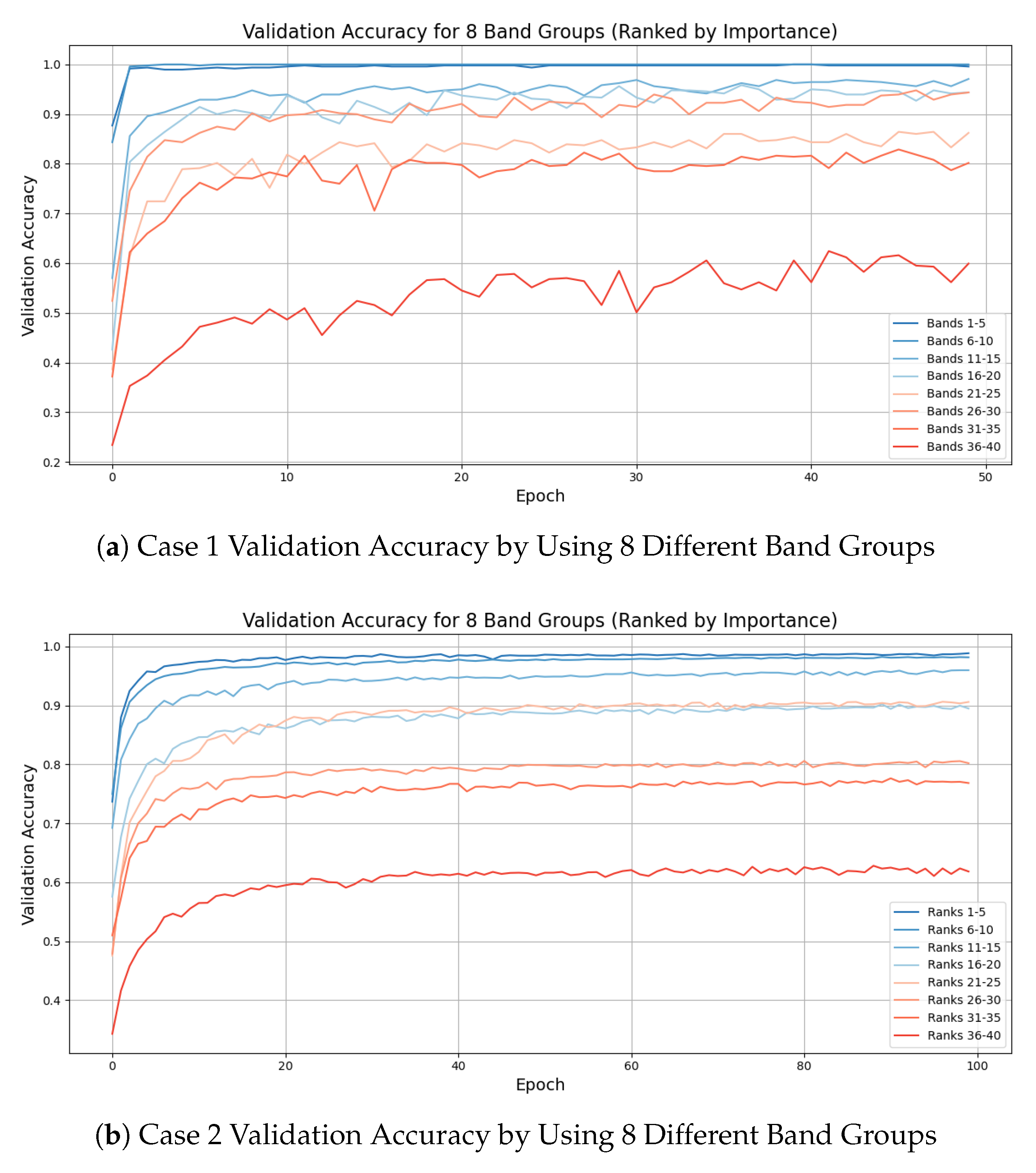
As discussed in the Section 2.2, the individual frequency bin importance scores were extracted using gain-based importance from the trained XGBoost classifier. After obtaining the gain score for each frequency bin, a sliding window approach with a stride of one bin was applied to aggregate the importance scores across contiguous frequency bands. To ensure non-overlapping selection, bands were iteratively selected by excluding any frequency band that overlapped with previously chosen ones. This process continued until the predefined number of most discriminative frequency bands was identified. To visualize the effect of using frequency bands with varying importance levels and to simplify computation, the sliding window technique was modified to use non-overlapping windows instead of a stride of one bin. This resulted in 40 non-overlapping frequency bands across the entire frequency spectrum. These bands were ranked in descending order of importance and then divided into 8 groups based on their ranked position. The model was trained 8 times, each time using one group of frequency bands as input features, and the validation accuracy results for each group are presented in Figure 10. In both cases, it can be observed that groups containing the highest ranked frequency bands (specifically ranks 1-5 and 6-10) achieved substantially higher validation accuracy. This result demonstrates that in both scenarios, the top five most relevant bands are sufficient to achieve high classification performance while maintaining computational efficiency. On the other hand, as lower ranked frequency bands were used, the model performance gradually degraded. This trend indicates that a limited number of selected frequency bands can preserve most of the information needed for DL models, leading to efficient input reduction while maintaining high performance. The results also reinforce the validity of the proposed band selection strategy across different rotating machineries.
Figure 8.
Selected Frequency Bands (Case 1)
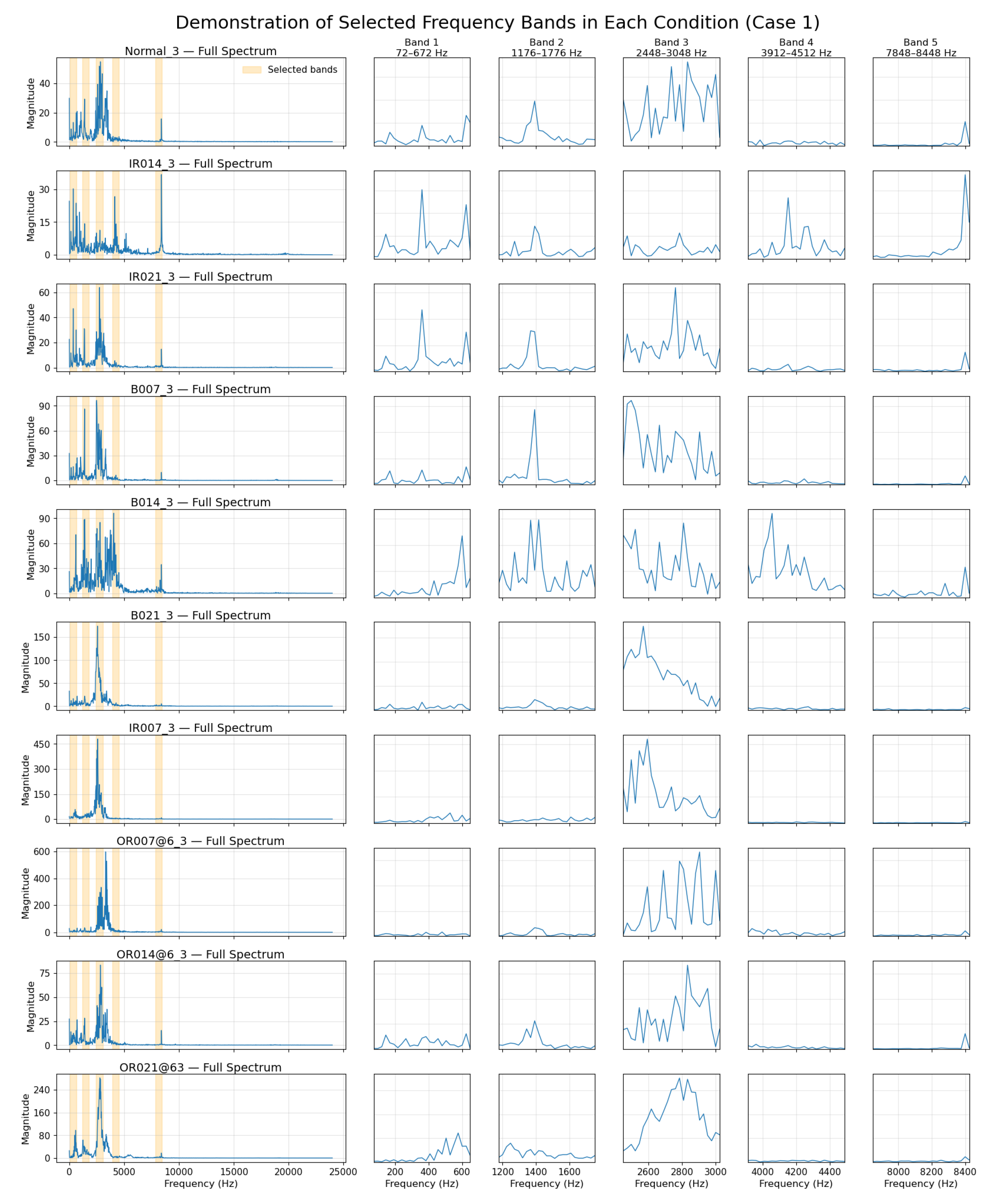
Figure 9.
Selected Frequency Bands (Case 2)
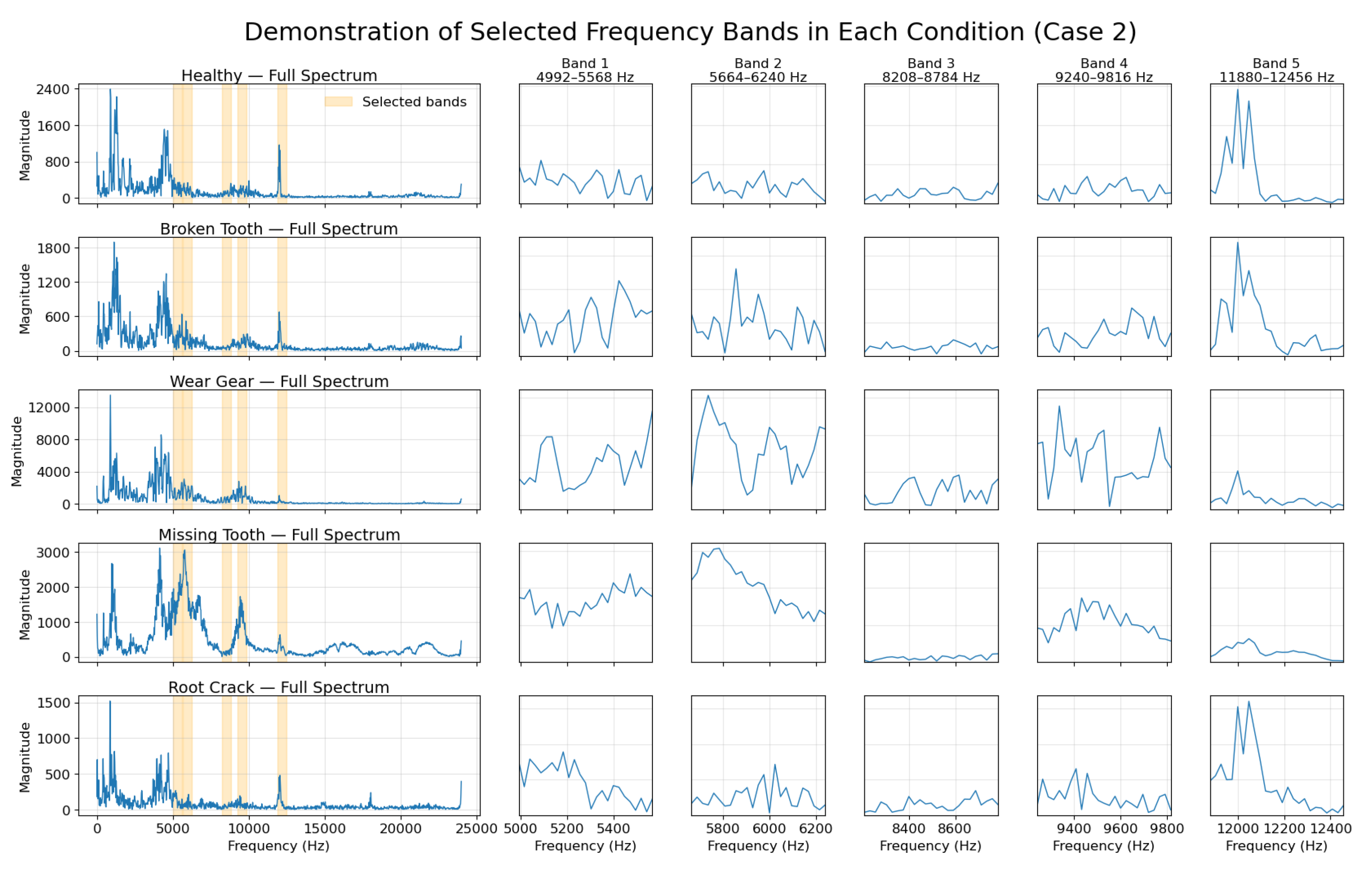
Figure 10.
(a) Case 1 Validation Accuracy by Using 8 Different Band Groups. (b) Case 2 Validation Accuracy by Using 8 Different Band Groups.
Figure 10.
(a) Case 1 Validation Accuracy by Using 8 Different Band Groups. (b) Case 2 Validation Accuracy by Using 8 Different Band Groups.
To further demonstrate the superior fault detection performance of the proposed method over existing machine learning approaches, a comparison with state-of-the-art machine learning-based fault detection techniques was conducted in the study. A summary of these techniques is presented in Table 5, highlighting their feature extraction strategies, model architectures, and reported classification accuracies. Among these techniques, an advanced Transformer model proposed in [43] that uses frequency features and a multi-scale encoder to capture both local and global fault patterns. With a custom cross-flipped decoder, the model achieved 99.85% accuracy. The method proposed in [44] combines wavelet packet decomposition with a DBN classifier, where DBN hyper-parameters are optimized using a chaotic sparrow search algorithm. Among these techniques, the method presented in [45] converts vibration signals into time–frequency images using variational mode decomposition and continuous wavelet transform, which are then classified through an improved CNN. This image-based approach enables spatial feature learning and achieves strong diagnostic performance across varying operating conditions. The approach described in [46] introduces a time-domain diagnosis model based on the KACSEN architecture, which leverages the Kolmogorov–Arnold framework for complex feature mapping. By integrating an attention mechanism, the model emphasizes informative signal components and performs effectively under different fault types. In [47], an end-to-end fault diagnosis framework combining a multi-scale CNN with LSTM layers is proposed, where the CNN extracts hierarchical features from both raw and down-sampled time-domain signals, and the LSTM captures temporal dependencies for final classification. Compared with these existing methods, the proposed model demonstrates strong performance in terms of accuracy, efficiency, and interpretability. Unlike approaches that depend on signal pre-processing, manual frequency localization, image conversion, or complex in-model computations, our method directly utilizes selected frequency bands. In our experiments, only 1/8 of the total frequency bands were selected and used for model training, significantly reducing the input size without compromising performance. The application of XGBoost for band selection ensures that only the most informative spectral regions are retained, effectively minimizing redundancy. Combined with a hybrid CNN–Transformer architecture, the model captures both local and global signal patterns with high effectiveness.
5. Concluding Remarks
This study proposed a frequency-domain fault classification framework that integrates FFT-based feature extraction, data-driven discriminative frequency band selection, and a CNN-Transformer hybrid model for classification. Feature extraction was carried out by applying the FFT to segmented sets of raw vibration signals. The obtained frequency spectra were then divided into multiple frequency bands, and XGBoost was employed to evaluate and rank the importance of each frequency band based on its contribution to classification accuracy. The top-ranked frequency bands were regarded as the most discriminative bands and subsequently fed into the hybrid DL model for fault classification.
To evaluate the effectiveness of the proposed framework, a series of experiments were conducted on two open datasets: the CWRU bearing dataset and the BJTU planetary gearbox dataset. Experimental results show that the CNN–Transformer classifier, utilizing the identified discriminative frequency bands, consistently outperforms existing literature approaches by achieving superior classification accuracy across diverse fault types and mechanical systems. This confirms that the combination of data-driven discriminative frequency band selection and DL holds strong potential for robust and efficient fault diagnosis.
However, the current frequency band identification method is restricted to one-dimensional features derived solely from the frequency spectra of vibration signals. Future work may explore extensions of this framework by incorporating higher-dimensional inputs, such as time-frequency representations, or by investigating multi-channel and feature-fusion techniques. These directions could enable the model to capture more complex temporal and spatial patterns, thereby enhancing its generalizability to real-world fault scenarios.
Author Contributions
Conceptualization, C.H., W.Y., O.G., and F.D.; methodology, C.H.; software, C.H.; validation, C.H.; formal analysis, C.H.; investigation, C.H.; resources, C.H.; data curation, C.H.; writing—original draft preparation, C.H.; writing—review and editing, C.H., W.Y., L.Z. and F.D.; visualization, C.H.; supervision, W.Y., O.G. and F.D.; project administration, W.Y.; funding acquisition, W.Y. All authors have read and agreed to the published version of the manuscript.
Funding
This research received no external funding.
Institutional Review Board Statement
Not applicable.
Informed Consent Statement
Not applicable.
Data Availability Statement
The Case Western Reserve University (CWRU) bearing dataset is publicly available online at https://engineering.case.edu/bearingdatacenter [41]. The Beijing Jiaotong University (BJTU) planetary gearbox dataset is also publicly available online: https://github.com/Liudd-BJUT/WT-planetary-gearbox-dataset [42]. No new data were created in this study.
Conflicts of Interest
The authors declare no conflicts of interest.
References
- Kong, K.; Dyer, K.; Payne, C.; Hamerton, I.; Weaver, P.M. Progress and Trends in Damage Detection Methods, Maintenance, and Data-driven Monitoring of Wind Turbine Blades – A Review. Renewable Energy Focus 2023, 44, 390 – 412. Cited by: 96; All Open Access, Hybrid Gold Open Access, . [CrossRef]
- Dibaj, A.; Gao, Z.; Nejad, A.R. Fault detection of offshore wind turbine drivetrains in different environmental conditions through optimal selection of vibration measurements. Renewable Energy 2023, 203, 161–176. [CrossRef]
- Badihi, H.; Zhang, Y.; Jiang, B.; Pillay, P.; Rakheja, S. A Comprehensive Review on Signal-Based and Model-Based Condition Monitoring of Wind Turbines: Fault Diagnosis and Lifetime Prognosis. Proceedings of the IEEE 2022, 110, 754 – 806. Cited by: 158; All Open Access, Hybrid Gold Open Access, . [CrossRef]
- Zhang, Q.; Su, N.; Qin, B.; Sun, G.; Jing, X.; Hu, S.; Cai, Y.; Zhou, L. Fault Diagnosis for Rotating Machinery Based on Dimensionless Indices: Current Status, Development, Technologies, and Future Directions. Electronics 2024, 13. [CrossRef]
- Tuirán, R.; Águila, H.; Jou, E.; Escaler, X.; Mebarki, T. Fault Diagnosis in a 2 MW Wind Turbine Drive Train by Vibration Analysis: A Case Study. Machines 2025, 13. [CrossRef]
- Wang, Y.; Liu, H.; Li, Q.; Wang, X.; Zhou, Z.; Xu, H.; Zhang, D.; Qian, P. Overview of Condition Monitoring Technology for Variable-Speed Offshore Wind Turbines. Energies 2025, 18. [CrossRef]
- Fang, C.; Chen, Y.; Deng, X.; Lin, X.; Han, Y.; Zheng, J. Denoising method of machine tool vibration signal based on variational mode decomposition and Whale-Tabu optimization algorithm. Scientific Reports 2023, 13, 1505. [CrossRef]
- Chen, B.; Hai, Z.; Chen, X.; Chen, F.; Xiao, W.; Xiao, N.; Fu, W.; Liu, Q.; Tian, Z.; Li, G. A time-varying instantaneous frequency fault features extraction method of rolling bearing under variable speed. Journal of Sound and Vibration 2023, 560, 117785. [CrossRef]
- Xu, Y.; Yan, X.; Feng, K.; Sheng, X.; Sun, B.; Liu, Z. Attention-based multiscale denoising residual convolutional neural networks for fault diagnosis of rotating machinery. Reliability Engineering & System Safety 2022, 226, 108714. [CrossRef]
- Alonso-Gonzalez, M.; Diaz, V.G.; Lopez Perez, B.; Cristina Pelayo G-Bustelo, B.; Anzola, J.P. Bearing Fault Diagnosis With Envelope Analysis and Machine Learning Approaches Using CWRU Dataset. IEEE Access 2023, 11, 57796 – 57805. Cited by: 38; All Open Access, Gold Open Access, . [CrossRef]
- Blockeel, H.; Devos, L.; Frénay, B.; Nanfack, G.; Nijssen, S. Decision trees: from efficient prediction to responsible AI, 2023. [CrossRef]
- Abdallah, I.; Dertimanis, V.; Mylonas, C.; Tatsis, K.; Chatzi, E.; Dervilis, N.; Worden, K.; Maguire, A. Fault Diagnosis of Wind Turbine Structures Using Decision Tree Learning Algorithms with Big Data. In Proceedings of the Proceedings of the 12th International Conference on Damage Assessment of Structures (DAMAS 2017), 06 2018, pp. 3053–3061. [CrossRef]
- Lipinski, P.; Brzychczy, E.; Zimroz, R. Decision Tree-Based Classification for Planetary Gearboxes’ Condition Monitoring with the Use of Vibration Data in Multidimensional Symptom Space. Sensors 2020, 20. [CrossRef]
- Shubita, R.R.; Alsadeh, A.S.; Khater, I.M. Fault Detection in Rotating Machinery Based on Sound Signal Using Edge Machine Learning. IEEE Access 2023, 11, 6665 – 6672. Cited by: 26; All Open Access, Gold Open Access, . [CrossRef]
- Alhams, A.; Abdelhadi, A.; Badri, Y.; Sassi, S.; Renno, J. Enhanced Bearing Fault Diagnosis Through Trees Ensemble Method and Feature Importance Analysis. Journal of Vibration Engineering & Technologies 2024, 12, 109–125. [CrossRef]
- Dwyer, K.; Holte, R. Decision Tree Instability and Active Learning. In Proceedings of the Machine Learning: ECML 2007; Kok, J.N.; Koronacki, J.; Mantaras, R.L.d.; Matwin, S.; Mladenič, D.; Skowron, A., Eds., Berlin, Heidelberg, 2007; pp. 128–139.
- Choudakkanavar, G.; Mangai, J.A.; Bansal, M. MFCC based ensemble learning method for multiple fault diagnosis of roller bearing. International Journal of Information Technology 2022, 14, 2741–2751. [CrossRef]
- Hemalatha, S.; Kavitha, T.; Anand, P. Effectiveness of Classification Techniques for Fault Bearing Prediction. In Proceedings of the 2022 6th International Conference on Electronics, Communication and Aerospace Technology, 2022, pp. 8–13. [CrossRef]
- Souza, V.F.; Cicalese, F.; Laber, E.S.; Molinaro, M. Decision trees with short explainable rules. Theoretical Computer Science 2025, 1047, 115344. [CrossRef]
- Nguyen, T.D.; Nguyen, T.H.; Do, D.T.B.; Pham, T.H.; Liang, J.W.; Nguyen, P.D. Efficient and Explainable Bearing Condition Monitoring with Decision Tree-Based Feature Learning. Machines 2025, 13. [CrossRef]
- Tian, J.; Jiang, Y.; Zhang, J.; Wang, Z.; Rodríguez-Andina, J.J.; Luo, H. High-Performance Fault Classification Based on Feature Importance Ranking-XgBoost Approach with Feature Selection of Redundant Sensor Data. Current Chinese Science 2022, 2, 243–251. [CrossRef]
- Lin, Z.; Fan, Y.; Tan, J.; Li, Z.; Yang, P.; Wang, H.; Duan, W. Tool wear prediction based on XGBoost feature selection combined with PSO-BP network. Scientific Reports 2025, 15, 3096. [CrossRef]
- Tama, B.A.; Vania, M.; Lee, S.; Lim, S. Recent advances in the application of deep learning for fault diagnosis of rotating machinery using vibration signals. Artificial Intelligence Review 2023, 56, 4667–4709. [CrossRef]
- Chen, Y.; Liu, X.; Rao, M.; Qin, Y.; Wang, Z.; Ji, Y. Explicit speed-integrated LSTM network for non-stationary gearbox vibration representation and fault detection under varying speed conditions. Reliability Engineering & System Safety 2025, 254, 110596. [CrossRef]
- Wang, R.; Dong, E.; Cheng, Z.; Liu, Z.; Jia, X. Transformer-based intelligent fault diagnosis methods of mechanical equipment: A survey. Open Physics 2024, 22, 20240015. [CrossRef]
- Zhu, Z.; Lei, Y.; Qi, G.; Chai, Y.; Mazur, N.; An, Y.; Huang, X. A review of the application of deep learning in intelligent fault diagnosis of rotating machinery. Measurement: Journal of the International Measurement Confederation 2023, 206. Cited by: 358, . [CrossRef]
- Alam, T.E.; Ahsan, M.M.; Raman, S. Multimodal bearing fault classification under variable conditions: A 1D CNN with transfer learning. Machine Learning with Applications 2025, 21, 100682. [CrossRef]
- Zhang, S.; Wei, H.L.; Ding, J. An effective zero-shot learning approach for intelligent fault detection using 1D CNN. Applied Intelligence 2023, 53, 16041–16058. [CrossRef]
- Han, S.; Yao, L.; Duan, D.; Yang, J.; Wu, W.; Zhao, C.; Zheng, C.; Gao, X. Intelligent condition monitoring with CNN and signal enhancement for undersampled signals. ISA Transactions 2024, 149, 124–136. [CrossRef]
- Vaswani, A.; Shazeer, N.; Parmar, N.; Uszkoreit, J.; Jones, L.; Gomez, A.N.; Kaiser, L.; Polosukhin, I. Attention is all you need. In Proceedings of the Advances in Neural Information Processing Systems, 2017, Vol. 2017-December, p. 5999 – 6009. Cited by: 88052.
- Kim, S.; Seo, Y.H.; Park, J. Transformer-based novel framework for remaining useful life prediction of lubricant in operational rolling bearings. Reliability Engineering & System Safety 2024, 251, 110377. [CrossRef]
- Ding, Y.; Jia, M.; Miao, Q.; Cao, Y. A novel time–frequency Transformer based on self–attention mechanism and its application in fault diagnosis of rolling bearings. Mechanical Systems and Signal Processing 2022, 168, 108616. [CrossRef]
- Han, Y.; Zhang, F.; Li, Z.; Wang, Q.; Li, C.; Lai, P.; Li, T.; Teng, F.; Jin, Z. MT-ConvFormer: A Multitask Bearing Fault Diagnosis Method Using a Combination of CNN and Transformer. IEEE Transactions on Instrumentation and Measurement 2024, PP, 1–1. [CrossRef]
- Lu, Z.; Liang, L.; Zhu, J.; Zou, W.; Mao, L. Rotating Machinery Fault Diagnosis Under Multiple Working Conditions via a Time-Series Transformer Enhanced by Convolutional Neural Network. IEEE Transactions on Instrumentation and Measurement 2023, 72, 1–11. [CrossRef]
- Ahmed, S.F.; Alam, M.S.B.; Hassan, M.; Rozbu, M.R.; Ishtiak, T.; Rafa, N.; Mofijur, M.; Ali, A.B.M.S.; Gandomi, A.H. Deep learning modelling techniques: current progress, applications, advantages, and challenges. Artificial Intelligence Review 2023, 56, 13521–13617. [CrossRef]
- Saeed, A.; Khan, M.A.; Akram, U.; Obidallah, W.J.; Jawed, S.; Ahmad, A. Deep learning based approaches for intelligent industrial machinery health management and fault diagnosis in resource-constrained environments. Scientific Reports 2025, 15, 1114. [CrossRef]
- Brigham, E.O.; Morrow, R.E. The fast Fourier transform. IEEE Spectrum 1967, 4, 63–70. [CrossRef]
- Chen, T.; Guestrin, C. XGBoost: A Scalable Tree Boosting System. In Proceedings of the Proceedings of the 22nd ACM SIGKDD International Conference on Knowledge Discovery and Data Mining, New York, NY, USA, 2016; KDD ’16, p. 785–794. [CrossRef]
- LeCun, Y.; Bottou, L.; Bengio, Y.; Haffner, P. Gradient-Based Learning Applied to Document Recognition. Proceedings of the IEEE 1998, 86, 2278–2324. [CrossRef]
- Vaswani, A.; Shazeer, N.; Parmar, N.; Uszkoreit, J.; Jones, L.; Gomez, A.N.; Kaiser, L.u.; Polosukhin, I. Attention is All you Need. In Proceedings of the Advances in Neural Information Processing Systems; Guyon, I.; Luxburg, U.V.; Bengio, S.; Wallach, H.; Fergus, R.; Vishwanathan, S.; Garnett, R., Eds. Curran Associates, Inc., 2017, Vol. 30.
- Case Western Reserve University Bearing Data Center. Bearing Data Center Website. https://engineering.case.edu/bearingdatacenter. Accessed: 2025-06-29.
- Liu, D.; Cui, L.; Cheng, W. A review on deep learning in planetary gearbox health state recognition: Methods, applications, and dataset publication. Measurement Science and Technology 2023, 35. [CrossRef]
- Hou, Y.; Wang, J.; Chen, Z.; Ma, J.; Li, T. Diagnosisformer: An efficient rolling bearing fault diagnosis method based on improved Transformer. Engineering Applications of Artificial Intelligence 2023, 124, 106507. [CrossRef]
- Zhao, F.; Jiang, Y.; Cheng, C.; Wang, S. An improved fault diagnosis method for rolling bearings based on wavelet packet decomposition and network parameter optimization. Measurement Science and Technology 2023, 35, 025004. [CrossRef]
- Gu, J.; Peng, Y.; Lu, H.; Chang, X.; Chen, G. A novel fault diagnosis method of rotating machinery via VMD, CWT and improved CNN. Measurement 2022, 200, 111635. [CrossRef]
- Jin, H.; Li, X.; Yu, J.; Wang, T.; Yun, Q. A bearing fault diagnosis model with enhanced feature extraction based on the Kolmogorov–Arnold representation Theorem and an attention mechanism. Applied Acoustics 2025, 240, 110903. [CrossRef]
- Chen, X.; Zhang, B.; Gao, D. Bearing fault diagnosis base on multi-scale CNN and LSTM model. Journal of Intelligent Manufacturing 2021, 32, 971–987. [CrossRef]
Figure 1.
Schematic of Proposed Method
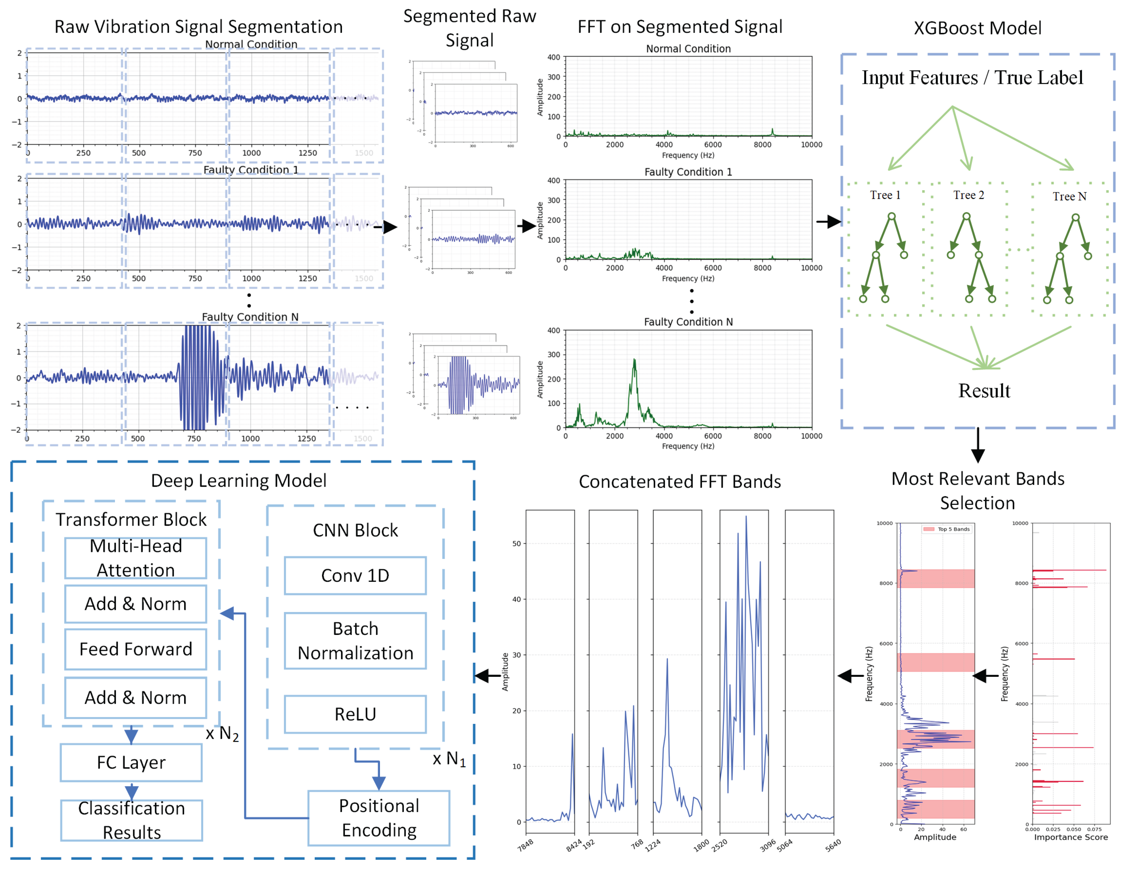
Figure 2.
(a) CWRU Experimental Setup. (b) CWRU Experimental Setup Schematic Diagram.
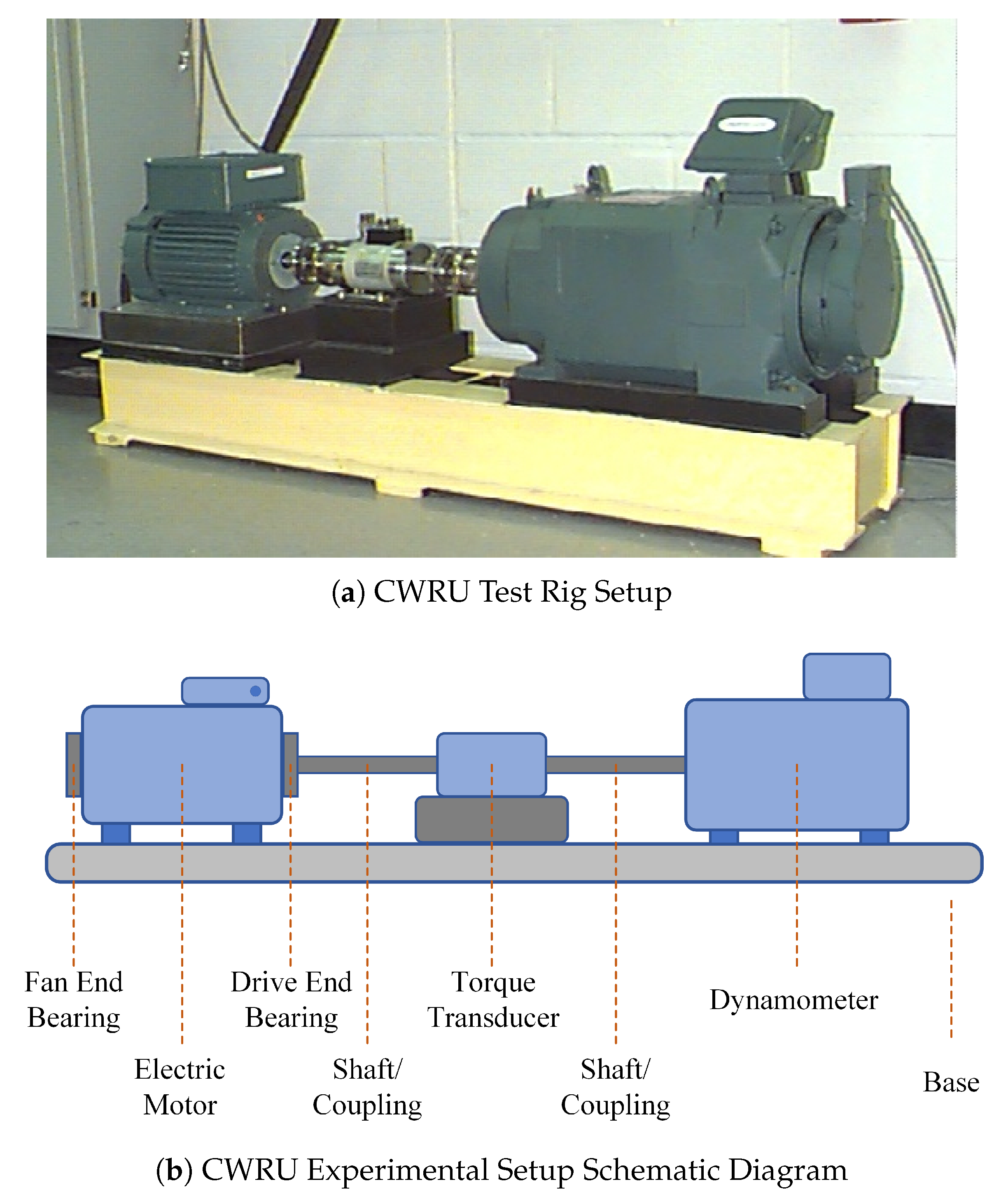
Figure 3.
CWRU Dataset: Segmented Signals and Their Frequency Spectra
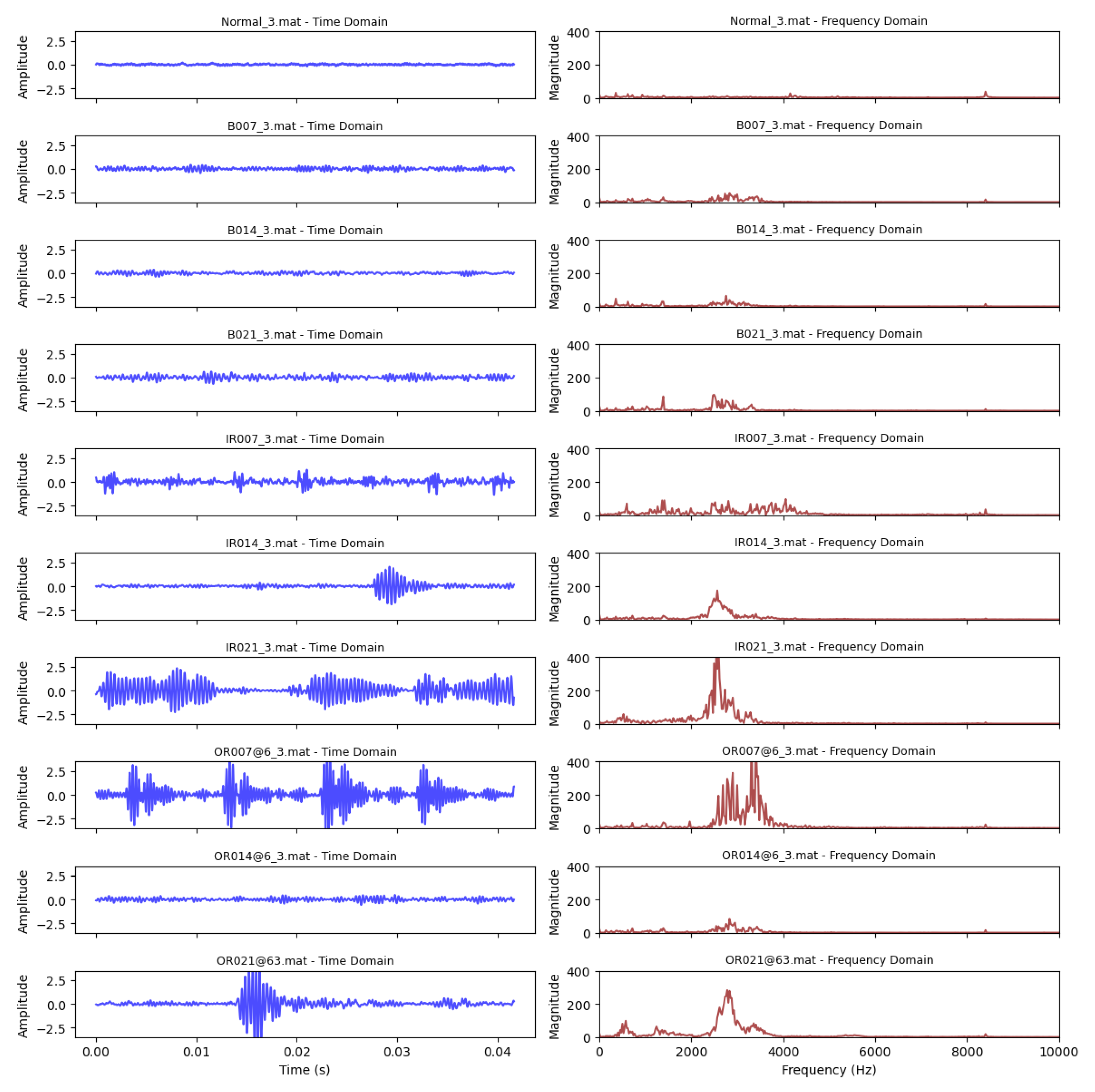
Figure 4.
BJTU Wind Turbine Planetary Gearbox Experimental Setup Schematic Diagram.
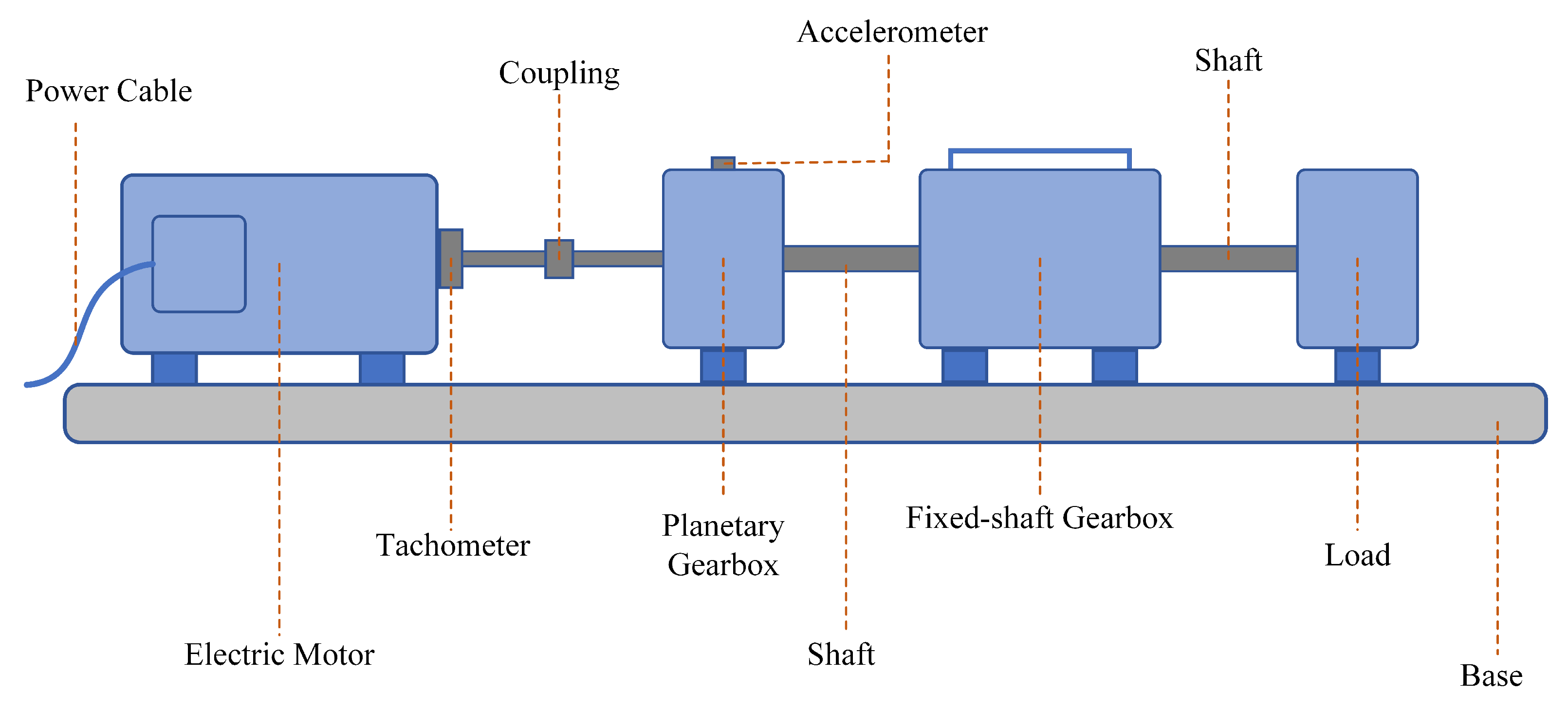
Figure 5.
BJTU Dataset: Segmented Signals and Their Frequency Spectra
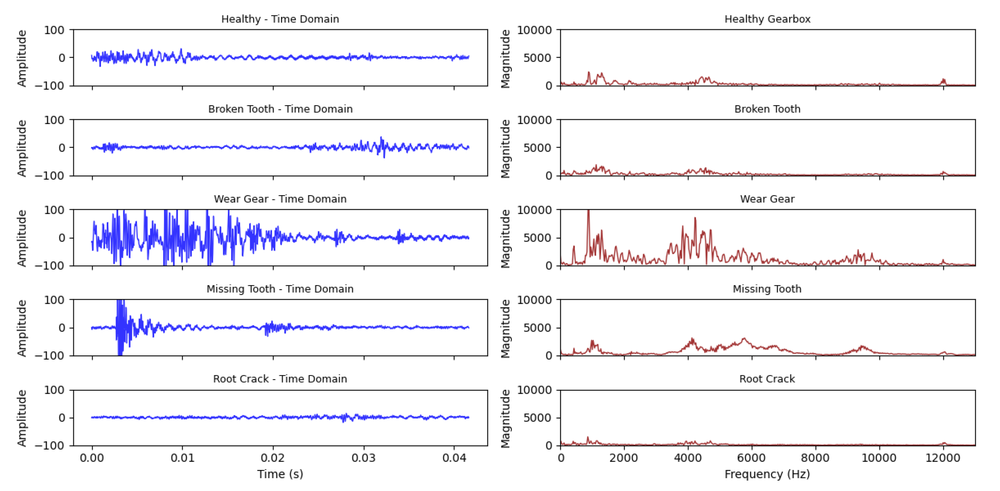
Figure 6.
(a) Model Performance Curves. (b) Confusion Matrix.

Figure 7.
(a) Model Performance Curves. (b) Confusion Matrix.
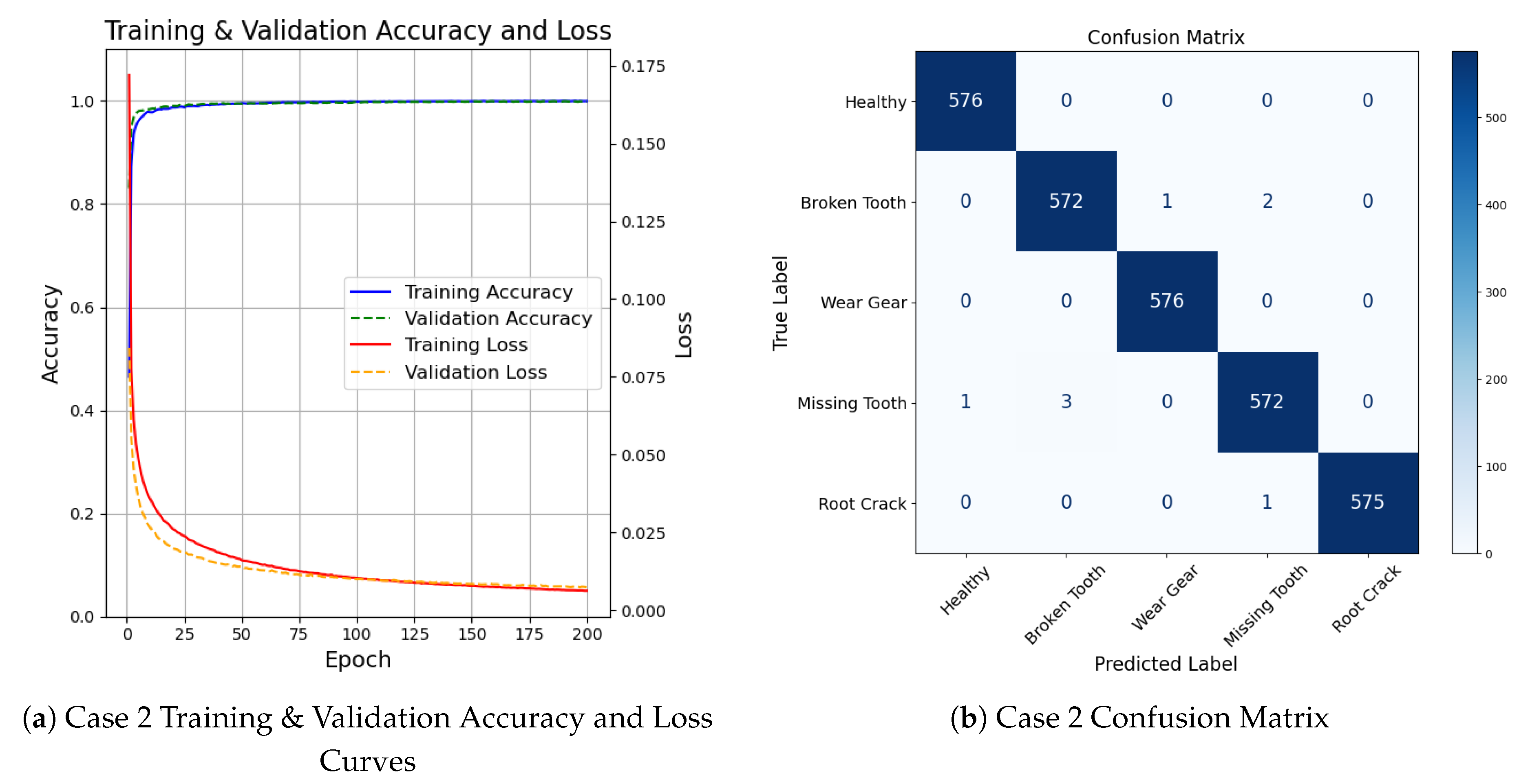

Table 1.
Description of fault index labels used in the CWRU dataset
| Index | File Name | Fault Type | Fault Size (mil) | Location |
|---|---|---|---|---|
| 0 | Normal_3.mat | Normal | – | – |
| 1 | B007_3.mat | Ball Fault | 7 | – |
| 2 | B014_3.mat | Ball Fault | 14 | – |
| 3 | B021_3.mat | Ball Fault | 21 | – |
| 4 | IR007_3.mat | Inner Race | 7 | – |
| 5 | IR014_3.mat | Inner Race | 14 | – |
| 6 | IR021_3.mat | Inner Race | 21 | – |
| 7 | OR007@6_3.mat | Outer Race | 7 | 6:00 |
| 8 | OR014@6_3.mat | Outer Race | 14 | 6:00 |
| 9 | OR021@6_3.mat | Outer Race | 21 | 6:00 |
Table 2.
Fault index mapping for sun gear conditions in the BJTU dataset
| Index | Condition | Description |
|---|---|---|
| 0 | Healthy | No damage on the sun gear |
| 1 | Broken Tooth | Partial removal (about one-third) of a sun gear tooth |
| 2 | Wear Gear | Gear tooth surface worn |
| 3 | Missing Tooth | Complete tooth removal |
| 4 | Root Crack | Crack introduced at the root of a sun gear tooth |
Table 3.
Frequency Bands Importance Scores - Case 1
| Band Rank | Frequency Range | Importance Scores |
|---|---|---|
| 1 | 7848–8448 Hz | 415.6893 |
| 2 | 2448–3048 Hz | 373.6769 |
| 3 | 1176–1776 Hz | 342.1831 |
| 4 | 72–672 Hz | 195.7419 |
| 5 | 3912–4512 Hz | 95.5129 |
| 6 | 3192–3792 Hz | 56.8888 |
| 7 | 1848–2448 Hz | 34.1304 |
| 8 | 5832–6432 Hz | 28.5478 |
| 9 | 9192–9792 Hz | 18.6156 |
| 10 | 7248–7848 Hz | 18.4222 |
| ... | ... | ... |
Table 4.
Frequency Bands Importance Scores - Case 2
| Band Rank | Frequency Range | Importance Scores |
|---|---|---|
| 1 | 8184–8784 Hz | 624.7955 |
| 2 | 4992–5592 Hz | 506.2124 |
| 3 | 9240–9840 Hz | 236.5562 |
| 4 | 11808–12408 Hz | 181.2200 |
| 5 | 5664–6264 Hz | 129.3388 |
| 6 | 1608–2208 Hz | 96.6329 |
| 7 | 4392–4992 Hz | 57.2291 |
| 8 | 0–600 Hz | 43.8308 |
| 9 | 6288–6888 Hz | 38.6528 |
| 10 | 816–1416 Hz | 38.0441 |
| ... | ... | ... |
Table 5.
Classification Performance Comparison on CWRU Bearing Dataset
| Study / Reference | Feature Type | Classifier | Accuracy (%) | Remarks |
|---|---|---|---|---|
| Hou et al. [43] | Frequency Domain | Improved Transformer | 99.85 | Transformer with multi-feature parallel fusion. |
| Zhao et al. [44] | WPD & Energy Features | WPD-CSSOA-DBN | 98.24 | Signal processing technique with energy feature selection and deep belief network. |
| Gu et al. [45] | Image | CNN | 99.90 | Signal pre-processing with image-based CNN classification. |
| Jin et al. [46] | Time Domain | KACSEN | 99.27 | Enhanced feature extraction with SE attention mechanism. |
| Chen et al. [47] | Time Domain | MCNN-LSTM | 99.31 | End-to-end fault classification model. |
| Proposed Method | Selected Frequency Bands | CNN + Transformer | 99.90 | High accuracy with frequency-band-based feature selection and hybrid classification. |
Disclaimer/Publisher’s Note: The statements, opinions and data contained in all publications are solely those of the individual author(s) and contributor(s) and not of MDPI and/or the editor(s). MDPI and/or the editor(s) disclaim responsibility for any injury to people or property resulting from any ideas, methods, instructions or products referred to in the content. |
© 2025 by the authors. Licensee MDPI, Basel, Switzerland. This article is an open access article distributed under the terms and conditions of the Creative Commons Attribution (CC BY) license (http://creativecommons.org/licenses/by/4.0/).
Copyright: This open access article is published under a Creative Commons CC BY 4.0 license, which permit the free download, distribution, and reuse, provided that the author and preprint are cited in any reuse.


