
Submitted:
02 November 2025
Posted:
04 November 2025
You are already at the latest version
Abstract
We investigate the fundamental tradeoff between entropy and Gini index within income distributions, employing a stochastic framework to expose deficiencies in conventional inequality metrics. Anchored in the principle of maximum entropy (ME), we position entropy as a key marker of societal robustness, while the Gini index, identical to the (second-order) K-spread coefficient, captures spread but neglects dynamics in distribution tails. We recommend supplanting Lorenz profiles with simpler graphs such as the odds and probability density functions, and a core set of numerical indicators (K-spread K₂/μ, standardized entropy Φμ, and upper and lower tail indices, ξ, ζ) for deeper diagnostics. This approach fuses ME into disparity evaluation, highlighting a path to harmonize fairness with structural endurance. Drawing from percentile records in the World Income Inequality Database over 1947–2023, we fit flexible models (Pareto–Burr–Feller, Dagum) and extract K-moments and tail indices. Results unveil a convex frontier: moderate Gini reductions have little effect on entropy, but aggressive equalization incurs steep stability costs. Country-level analyses (Argentina, Brazil, South Africa, Bulgaria) link entropy declines to political ruptures, positioning low entropy as a precursor to instability. On the other hand, analyses based on the core set of indicators for present-day geopolitical powers (China, India, USA and Russia) show that they are positioned in a high stability area.
Keywords:
entropy
; principle of maximum entropy
; K-moments
; stochastics
; wealth
; income profiles
; Gini index
; stability
| κατὰ μὲν τὴν οὐσίαν καὶ τὸν λόγον τὸν τὸ τί ἦν εἶναι λέγοντα μεσότης ἐστὶν ἡ ἀρετή, κατὰ δὲ τὸ ἄριστον καὶ τὸ εὖ |
| ἀκρότης. (In terms of its essence and the definition of its nature, virtue is the mean, but in terms of excellence and rightness, [virtue is] |
| the extreme; Aristotle [1]) |
1. Introduction
Our previous research (Koutsoyiannis and Sargentis [2]) delineated entropy's role across physical and economic systems. Extending this, here we investigate the dynamics between entropy and Gini coefficient across income structures.
The Gini index, here reformulated as the second-order K-moment standardized by the mean, (see Section 3.1.3), and referred to as the K-spread coefficient, leads inequality assessments. Still, it masks extremes, i.e., the tail behaviour of the distributions: profiles with matching Gini index can show stark contrasts in income extremes. Entropy instead gauges overall variability and uncertainty and, through the principle of maximum entropy (ME), spots the likeliest—and, hence, most resilient—structure under given constraints. The ME principle was originally formalized by Jaynes [3] as a method to infer the most probable distribution given constraints. In economic contexts, ME posits that income distributions tend toward states of maximum entropy under real-world constraints.
The key conjecture in this study is that income profiles would naturally tend toward peak entropy given real constraints. On the other hand, pushing the economic state to depart from the peak entropy and creating large and persistent deviations from it, herald fragility. Hence, a scale-invariant entropy measure, or standardized entropy, [2], functions as a resilience gauge, complementing as a spread gauge.
Under constraints of specified mean, , and K-spread (Gini), , we demonstrate here that entropy maximization results in a generalized half logistic (GHL) distribution, a limiting case of which is the exponential distribution. The latter materializes the peak entropy pole, as (. The distance from this pole is another measure of resilience or stability of an economy, with small distance denoting small instability.
To ratify the key conjecture, we use data (percentile records) from the World Income Inequality Database (WIID), to which we fit flexible models (Pareto–Burr–Feller, Dagum) and extract K-moments and tail indices. We perform country-level analyses (Argentina, Brazil, South Africa, Bulgaria) to test whether entropy declines can be linked to political ruptures. In addition we analyse the core set of indicators in present-day geopolitical powers (China, India, USA and Russia, EU) to assess their stability based on the criteria developed.
2. Data
The real-world applications in this study are based on the World Income Inequality Database [4,5], developed and maintained by the United Nations University World Institute for Development Economics Research. More specifically, the product used is the WIID Companion Country Dataset, which reports inequality data by country. This was selected because of its unparalleled comprehensiveness and global scope in providing income inequality statistics. The dataset encompasses 202 nations (including 4 historical entities), starting in 1947 (for USA; later for other countries) and extending to 2023, offering 2546 distinct country-year records. This broad coverage enables detailed analyses of inequality trends across diverse geopolitical contexts and historical eras, which is essential for our examination of the tradeoff between entropy and the Gini index. WIID allows us to explore extreme Gini values and long-term patterns in countries like Argentina, Bulgaria, Brazil, and South Africa, as well as in major geopolitical powers such as the USA, China, EU, Russia and India, ensuring a robust empirical foundation for applying theoretical stochastic tools to real-world income disparities.
A key reason for choosing WIID is its provision of percentile-based income data, which aligns perfectly with the methodological requirements of our research. The specific data used are those named “p1”–“p100”, which represent the income per capita (based on GDP) per percentile, standardized so as to have an average of 1.These facilitate the calculation of Lorenz curves, Gini indices, and entropy measures directly. This granularity in percentiles supports our use of K-moments, ME principle, and tail index estimations, allowing for precise comparisons between relevant probabilistic distributions. Unlike more aggregated datasets, WIID’s percentile-level detail enables us to handle grouped data effectively, reliably estimate empirical statistics, and visualize tradeoffs in figures.
WIID’s reliability and methodological rigour enable comparability across countries and over time. Curated by inequality experts, the database incorporates adjustments for data quality and consistency, with transparent documentation in user guides, technical notes, and replication tools. This minimizes biases in cross-national comparisons, which is critical for our analysis of social stability and political histories in case studies. Widely recognized in academic research for monitoring global inequality trends, WIID outperforms alternative sources by offering both raw and processed data, ensuring that our findings on the limitations of the Gini index and the advantages of entropy-based approaches are grounded in high-quality, verifiable evidence.
3. Methods
3.1. Basic Stochastic Tools
3.1.1. Distribution Function and Relative Concepts; Expectation and Moments
Let be a stochastic (random) variable of continuous type (i.e., taking on values that are real numbers); notice that we underline stochastic variables to distinguish them from regular variables. We denote its distribution function (i.e. probability of non-exceedance) and its tail function (i.e. probability of exceedance), respectively, as:
where P denotes probability. A useful derived function is the so-called odds function:
Both and are nondecreasing functions, and since the variable is continuous, the inverse functions exist. The inverse of , denoted as is called the quantile function. The derivative of the distribution function:
is the probability density function and obeys the obvious relationship:
Any deterministic function of , , is a stochastic variable per se, because its argument is stochastic. The expectation of the stochastic variable is defined as:
For and we get, respectively, the mean, , and the variance, , of :
The variance is necessarily nonnegative and its square root, , is the standard deviation. For nonnegative variables, the limit in the above integrals is replaced by 0, while the ratio , termed the coefficient of variation, is a useful dimensionless index of the variability of a system.
3.1.2. Entropy and Standardized Entropy
It is possible to define a function in terms of not the variable but the probability density per se, i.e. , where is any specified function. Among the several choices of , most useful is the logarithmic function, which results in the definition of entropy, . The emergence of the logarithm in the definition of entropy follows some postulates originally set up by Shannon (1948, [6]) for stochastic variables of discrete type. Extension for a continuous stochastic variable was not contained in Shannon’s original work but was given later (see e.g. [7 (p. 375),8]) as:
where is a background measure that can be any probability density, proper (with integral equal to 1, as in equation (4)) or improper (meaning that its integral diverges). Typically, it is an (improper) Lebesgue density, i.e. a constant. We note that most texts do not include the background measure in the definition (or set ) but in terms of physical consistency this is an error, because in order to take the logarithm of a quantity, this quantity must be dimensionless. The density function has units and therefore we need to divide it by a quantity with same units before taking the logarithm. Even if we choose the Lebesgue measure as background, with (constant), where is the unit used to measure , still the entropy depends on the unit. It can easily be verified that if we measure with two different units and , the respective entropies and will differ by a constant:
The entropy per se is always dimensionless and for continuous variables it can be either positive or negative, depending on the assumed , ranging from to a maximum value, depending on the system and, in particular on its constraints.
Entropy is generally a measure of uncertainty and its importance lies on the principle of maximum entropy, formally introduced in 1957 by Jaynes [3]. This postulates that the entropy of a stochastic system should be at maximum, under some conditions, formulated as constraints, which incorporate the information that is given about this system. The meaning of the principle is that the maximum entropy state of a system is the most probable one that is allowed by its degrees of freedom and not disallowed by its constraints. Therefore, entropy is also a measure of stability: a state that is far apart the maximum entropy state is unstable as it will tend to change toward maximizing entropy. The principle can be used for logical inference as well as for modelling physical systems. In this respect, the tendency of entropy to become maximal (as in the Second Law of thermodynamics), which drives natural change, can result from this principle. On the other hand, the principle equips the entropy concept with a powerful tool for logical inference.
In application in economics [2,9], for a constant background density equal to the inverse of the monetary unit (i.e. equal e.g. to 1 $) the entropy provides a measure of society’s wealth (even if expresses income). If we set the background measure to the value is the mean income, we get the standardized entropy which from equation (8) is obtained as
This quantity, which cannot exceed a maximum value of 1 for nonnegative continuous variables (see Section 3.3), has been originally introduced [2,9] as an index of inequality. However, as we will see below, it can better be thought of as a measure of stability, while the notion of K-moments (see next) can better characterize inequality.
3.1.3. K-Moments
While in classical statistics moments of order higher than 2 are defined and used (by substituting , for in Equation (6)), these cannot be reliably estimated from samples [10]. However, the concept of knowable moments or K-moments [10] can reliably provide estimates for high-order moments.
The K-moments are defined as follows. We consider a sample of a stochastic variable , i.e., a number of independent copies of the stochastic variable , i.e., . If we arrange the variables in ascending order, the ith smallest, denoted as is termed the ith order statistic. The largest (pth) order statistic is:
and the smallest (first) is
We define the upper knowable moment (K-moment) of order p as the expectation of the largest of the p variables :
and the lower knowable moment (K-moment) of order p as the expectation of the smallest of the p variables :
An important property, directly resulting from their definition, is that the K-moments are ordered as follows:
These moments are noncentral and we can also define central moments as
As shown in [10 (chapter 6)], for a stochastic variable of continuous type, the upper K-moment of order p of , is theoretically calculated as:
Likewise, the lower K-moment of order p is theoretically calculated as:
The unbiased estimator of the upper K-moment from a sample of size is
and that of the lower K-moment is,
where
and is the gamma function. For data that are grouped in classes the resulting modified estimator is shown in Appendix A.3.
Based on the K-moments, we define the K-centre of order , , and the K-spread of order , , as:
where . The least-order meaningful values thereof are:
Since [10], we have , i.e., the first and second order K-centre parameters are equal to each other and equal to the mean. The standardized parameter
is a characteristic spread index, similar to the coefficient of variation used in classical statistics, and will be referred to as the K-spread coefficient. Furthermore, the standardized parameter is also a spread index which will be referred to as the K-spread ratio of order .
3.1.4. Specific Distribution Functions and Tail Indices
Here we use several distribution functions resulting from entropy maximization, which are summarized in Table 1, along with their characteristics. Among them, the three-parameter distributions, namely the Pareto-Burr-Feller (PBF) and the Dagum distributions are quite flexible and can describe most real-world systems. The Pareto, Weibull and exponential distribution are special cases of the PBF distribution. The logistic and the generalized half logistic (GHL) constitute another form of distribution, resulting from entropy maximization with constrained mean and K-moment of order 2.
In all distributions listed in Table 1, is a scale parameter with dimensions identical to those of the variable , and and are dimensionless parameters, representing the upper and lower tail indices, respectively. For a variable with domain , their definitions are based on the limiting relationships:
where and are nonzero and finite constants. Both can be also determined from the odds function by
where denotes the log-log derivative (LLD) of the odds function, defined as
The tail indices are important characteristics of a distribution. A distribution with upper tail index (e.g. the exponential) is light-tailed, while one with is a heavy tailed distribution. In a distribution with , the density is necessarily a decreasing function, at least close to the origin, with . In contrast. when , the density is an increasing function close to the origin, with , and is usually bell-shaped. The particular case is characteristic of the exponential and Pareto distributions, where is finite and the density is a decreasing function.
3.2. The Lorenz curve and the Gini Index
The economics literature makes extensive use of the Lorenz curve and the Gini index. If is the quantile function of a probability distribution, then the Lorenz curve is simply its integral standardized by the mean, i.e.,
The Gini index is the ratio of the area between the equality line and the Lorenz curve to the area under the equality line (which is 1/2), i.e.,
where to obtain the rightmost result, we observe that . It is easily shown (see Appendix A.2) that the Gini index is simply the K-spread coefficient:
Once we know the K-spread coefficient and the tail indices of a distribution, we can effectively approximate it by the following proposed relationship:
where
As shown in Appendix A.2, the approximation preserves the mean and moment, and the two tail indices of the exact distribution. Figure 1 shows that the above approximation is almost perfect for the PBF distribution. Appendix A.2 shows cases where the approximation is exact. Figure 2 shows a similar behaviour of the approximation for the Dagum distribution.
Therefore, one can replace the Lorenz curve altogether with three parameters, . Actually, these three parameters provide much richer information than the Lorenz curve per se. This is illustrated in Figure 3, which compares two distributions with very different behaviour, a PBF and a Dagum, which have the same but different tail indices. It is seen that the Lorenz curves do not give any indication of the different behaviours of the two distributions.
For this reason, we contend that the Lorenz curve, despite its popularity, is not a useful tool to understand the income distribution. A better tool, visualizing the distribution behaviour is the double logarithmic plot of the odds function, also seen in Figure 3, along with plots of the density function, in linear or logarithmic axes. All three additional plots do not hide the information of the differences, with the logarithmic plots also visualizing the tail indices.
Additional evidence that the Lorenz curve is not a truthful stochastic tool is provided by Figure 4, which is based on actual income distribution data for Bulgaria in 1971. (Nb., we investigate Bulgaria in more detail in Section 4.3.4.) The Lorenz curve is smooth and provides no information on the peculiarity of the income distribution in this case. Specifically, the density function plot shows that there is a huge peak at an income slightly lower than the mean, suggesting that most of the population had income close to this value. The Lorenz curve totally hides this fact, which is visible in the probability density plot, as well as in the odds function plot. In the latter, it appears as a big plateau at an income slightly lower than the mean, and at odds values around 1.
For these reasons, while for completeness we occasionally show some Lorenz curves in our applications, we do not recommend their use and we strongly propose the odds function double logarithmic plot as a replacement.
3.3. Maximum Entropy Distributions
Using calculus of variation, we can determine which is the probability density that maximizes the entropy, defined in Equation (7), under given constraints. If there is no constraint about the system, apart from the range where the variable lies, specified by the inequality constraint:
then, maximization of entropy results in uniformity, i.e. , while the maximum entropy, the standardized maximum entropy and the K-spread coefficient are:
However, a system becomes more interesting when, in addition to inequality constraints like (32), or even in absence of them, there appear equality constraints, corresponding to the information that is known about a system represented by the variable . In studying the material wealth (or income) in a certain society we assume two characteristic quantities: the mean μ, which is related to the total energy available to the society [2], and an upper limit of wealth (or income) , which is mainly determined by the available technology (knowhow) and thus we call it technological upper limit.
The constraints for entropy maximization are thus:
Assuming a Lebesgue background measure with , with λ being a monetary unit (e.g. λ = 1 $), the entropy maximizing probability density is [2]:
which is a (doubly) bounded exponential distribution. The particular characteristics of the distribution are given in Table 1. Illustrations of the density function for two values of the upper bound are seen in Figure 5 (left). In addition, Figure 5 (right) shows the variation of the mean, K-spread coefficient and standardized entropy, with the upper limit . All three quantities increase with the increase of , the K-spread coefficient tends to the value and the standardized entropy tends to .
As the tendency of entropy is to grow, one may understand that human societies would push the technological limit to high values and this has actually happened historically. In other words—and despite the bad name of entropy because of misunderstanding its meaning—the tendency of entropy to become maximal is the agent of change and technological progress. As seen Figure 5 (right), once the technological limit became high enough, say , it could be neglected as if . In this case we obtain the standard (unbounded) exponential distribution, also shown in Table 1. The characteristics of the latter distribution, namely K-spread coefficient and standardized entropy , define a characteristic point or a pole on a 2D plane () which (provided that our variable is nonnegative) cannot be surpassed in the sense that cannot take any value higher than 1, and the highest value of 1 can be achieved only if ; otherwise it would necessarily be smaller. Hence the distance of a specific country’s state from this pole, i.e.,
is a useful index for the characterization of an economy’s state, additional to those already discussed.
It can be shown (and confirmed in Figure 5, right) that, as , the K-spread coefficient tends to the value and the standardized entropy tends to . This signifies a uniform distribution (see Equation (33)). Furthermore, even though not shown in Figure 5, Equation (35) allows for values and in this case we have the (bounded) anti-exponential distribution. As , the mean , the K-spread coefficient tends to the value and the standardized entropy tends to . This signifies a distribution with all probability mass concentrated at (an impulse). The impulse represents certainty, with full equality of the population in economic terms. Stochastically, the reason for the emergence of these types of distribution, which must have been materialized in the far distant past at the cradle of human societies, is the very low technological limit, which did not allow any options for diversity in income. Interestingly, Marx and Engels [11] and their followers interpreted this situation of misery as representing an ancient classless society, and envisaged recreating it in the future.
At a next step, we pose an additional constraint, namely of a fixed K-spread coefficient, or equivalently a fixed moment. In this case, the determination of the resulting entropy maximizing distribution is cumbersome and is given in Appendix A.3. The result, if the domain of the variable is the entire line of reals, is the logistic distribution:
where is a parameter. If , as in the case of income, the resulting distribution is the generalized half-logistic (GHL), whose expression is
It can be easily verified that if , in the case of Equation (37) we get the standard logistic distribution, while in that of the Equation (38) the distribution becomes identical to the exponential one. Thus the GHL distribution contains the exponential distribution as a special case.
The details of both distributions are contained in Table 1. In the case of GHL, the equation giving the K-spread coefficient, albeit simple, cannot be solved explicitly for the parameter , yet, ifis known. it is easy to find numerically and then determine the standardized entropy from . A good analytical approximation of is given by
and of standardized entropy by
The thus established relationship between is illustrated in Figure 6 (curve named “exact ME GHL distribution”), which also shows the satisfactory behaviour of the approximation in Equation (40) (curve named “explicit ME GHL approximation”).
This relationship represents the tradeoff between entropy and K-spread coefficient (Gini index). As departs from the pole (point (1/2,1)) the entropy decreases in a symmetrical manner around the line . Points below the curve of Figure 6 are mathematically (and practically) feasible, while those above the curve are infeasible. Values indicate low stratification of society, in terms of income, and values indicate high stratification. As per entropy, we have (arbitrarily) partitioned the area below the curve of Figure 6 into three parts, based on the distance from the pole . Values of between 2/3 and 1 indicate high stability of economy, those between 1/3 and 2/3 indicate low stability, and those below 1/3 indicate high instability. The latter area also includes negative entropy values, which in reality are feasible, but not quite common.
As will be seen below, while the curve Figure 6 effectively captured the feasible space of the covariation of entropy and K-spread, the underlying GHL distribution proves not appropriate for modelling the income distribution. The main obstacle is its tail indices, which are , , same as in the exponential distribution. In reality, however, any deviation from the exponential distribution is due to different tail indices, rather than due to different K-spread with same tail indices. For this reason, it is useful to approximate the curve of Figure 6 with more general distributions, such as PBF and Dagum, as well as special cases thereof, such as Pareto and Weibull. As seen in Figure 6, which also compares the exact and approximate curves, and in Figure 7 (left) which shows the approximation errors, all four distributions provide good approximations. Figure 7 (right) shows that in the approximating distributions, the tail indices are no longer , but vary depending on the K-variation coefficient.
Most promising are the approximations by the two-parameter distributions Weibull and Pareto. The Weibull distribution provides good approximation for the low stratification part of the curve (). The upper tail index is , while the required value of the lower tail index and the achieved standardized entropy are:
The Pareto distribution provides good approximation for the high stratification part of the curve (). The lower tail index is , while the required value of the upper tail index and the achieved standardized entropy are:
4. Application
4.1. General Setting
Here we apply the framework theoretically developed in section 3 to income data of several countries and different periods. This application has two parts. In the first we examine the characteristics of four of the major geopolitical powers, USA, China, India, Russian Federation, and European Union for the year 2022, which is the most recent year for which all five have full data coverage.
In this second part, we examine the history of the evolution of two major economic indices, the K-spread (Gini index) and standardized entropy, as well as the distance from the pole of maximum entropy for four other countries, in correlation with the political history of each of them. These countries were chosen for the peculiarities in their politico-economic evolution, provided that their data also exhibit sufficient historical depth. Specifically, Argentina (1953–2023) was selected as a case study of a country that experienced successive military coups and political turmoil during the period 1953–1980. Bulgaria was chosen as an example of a Soviet satellite state attempting to implement the communist system and an egalitarian income distribution. Brazil was included as a country that, despite its severe inequalities, has historically recorded Gini values near 1/2. Finally, South Africa was selected due to its pronounced economic disparities and its persistent and extremely rigid social stratification.
A brief political overview of each country under examination is provided, beginning from a brief history and the political landscape to the time series examined. This allows us to form a concise understanding of broader societal perceptions regarding social stratification in different regions. Even if the available data for our analysis refer mainly to the second half of the 20th century and the early years of the 21st century, with these tools, we are trying to evaluate the social dynamics and the historical evolution of each country.
In all cases, from the available data all information referred to in Section 3 was extracted but presented only partly to avoid a very long text. The processing of the data is described in Appendix A.4 for the assignment of empirical values of the distribution function and density function for observed values of the income (given in percentiles), and in Appendix A.5 for the calculation of empirical values of entropy. The PBF and Dagum distributions were fitted in all cases, and the numerical values of indices were calculated both directly from the data and indirectly from the fitted distribution. The direct and indirect values were very similar and hence only the former are reported here. We note though that in extreme cases of large deviations of data from the two distributions, like in Bulgaria, 1971, shown in Figure 4, the direct empirical values differ from the indirect ones.
4.2. The Status of the Major Geopolitical Powers in 2022
In 2022, major geopolitical powers exhibited distinct perceptions of inequality shaped by historical legacies, economic structures, and policy approaches, influencing their social and political landscapes [12,13]. The United States framed inequality as a consequence of market-driven innovation, with policymakers often downplaying wealth concentration among the top 1% while public discourse highlighted racial and economic divides, amplifying polarization [14,15]. On the other hand, China’s leadership viewed inequality as a manageable byproduct of rapid growth since the 1978 reforms, prioritizing urban development and poverty reduction while tolerating wealth concentration among elites, with the “common prosperity” initiative signalling a shift toward addressing urban-rural disparities through targeted redistribution [16,17].
India perceived inequality as a structural challenge rooted in colonial land systems and informal economies, with elites accepting stark wealth gaps as a tradeoff for growth, though public frustration over stagnant wages and urban-rural divides fuelled demands for reform without cohesive policy action [18,19]. The European Union saw inequality as a threat to social cohesion, emphasizing robust welfare systems and progressive taxation to ensure equitable income distribution, though regional variations and crises like inflation sparked debates over deeper fiscal unity [20]. Russia perceived inequality as secondary to state stability, with economic measures boosting lower incomes but elite wealth concentration and regional disparities accepted as entrenched features of its resource-driven system [21].
Detailed graphs of the economic status (similar to those for Bulgaria of Figure 4) are given in Figure 8 for the USA and in Figure 9 for China. The graphical depictions show a close similarity between the two cases, with the most visible difference being the smaller upper tail index of China, visualized by the slope of the rightmost part of the odds function curve.
The K-spread vs. standardized entropy curve for all five geopolitical powers examined are shown in comparison to each other and to the GHL curve in the upper left panel of Figure 10, while in the upper right graph the distances from the pole of maximum entropy are compared. For completeness, the same graph in its lower panels provides information on the gross domestic product (GDP) per capita and gross domestic product based on purchasing power parity (GDP-PPP) per capita. These are important indices of prosperity, but they were not investigated in detail here, as the focus is on (in)equality and (in)stability of economy.
Observing the position of the geopolitical players in 2022 from the perspective outlined in the methodology above, we see that the K-spread coefficient (Gini index) does not reflect China’s political intentions regarding common prosperity, since it appears rather high. In contrast, evaluation through entropy captures the social dynamics more accurately, as China appears to be the most stable of all players, exhibiting the smallest distance from the pole of maximum entropy. India, although positioned according to the Gini index as having the potential to achieve maximum entropy, does not succeed in remaining close to the pole. The United States are at a greater distance than China and India, yet still within a stable framework; Russia is located at the boundary of high stability, while the European Union lies at the area of low stability.
In addition, Table 2 summarizes the main numerical indices resulted from this analysis. The lowest or highest values of the indices that favour equality or stability are highlighted in bold and it can be seen that China and Russia are the most notable in this respect.
4.3. A Brief Political History and the Evolution of Economic Indices in Specific Countries
4.3.1. Argentina
Argentina’s political history began with independence from Spain in 1816, leading to a period of civil wars between federalists and unitarians, eventually stabilizing under a federal constitution in 1853. The late 19th century saw economic prosperity driven by agricultural exports and European immigration, but also rising social tensions and oligarchic rule, culminating in the 1916 introduction of universal male suffrage and the Radical Civic Union’s ascent. The 1930 military coup marked the start of instability, followed by the 1943 coup that propelled Perón to power in 1946, establishing Peronism as a transformative force blending populism and authoritarianism [24].
In the 1950s, Argentina’s political and social perceptions were profoundly shaped by Peronism, a dominant political culture, emphasizing social justice, economic independence, and political sovereignty as a “third way” between communism and capitalism. Argentines under Peronism sought a balanced system that incorporated elements of state intervention in the economy without full communist collectivization, fostering a populist identity that prioritized national sovereignty over ideological extremes [25,26].
From 1950s to 1980s, Argentina experienced recurrent military interventions, including the 1955 coup that ousted Perón, the 1962 and 1966 coups against civilian governments, and the 1976 coup that initiated the brutal Dirty War under a military junta [27]. This era saw alternating periods of restricted democracy and outright dictatorship, and social unrest (Figure 11). The frequent upheavals stemmed from deep-seated political polarization, economic volatility including hyperinflation and debt crises, and a tradition of military involvement in politics [28].
Since the return to democracy in 1983, Argentina’s political history has been characterized by efforts to consolidate democratic institutions amid economic challenges [29]. In 1990s neoliberal reforms were introduced, followed by the 2001-2002 economic collapse and a series of short-lived presidencies. The period 2003-2015 saw progressive policies and debt restructuring, followed by shifts toward market-oriented reforms [30] and libertarian austerity measures, reflecting ongoing struggles for stability in a polarized landscape [31].
Observing Argentina’s history from the perspective outlined in the methodology above, we can see that the Gini index does not provide us with information regarding the stability and condition of social inequalities. Before 1980, this index ranged between 0.32–0.41 with an average value of 0.35; during 1980–1999 it ranged between 0.38–0.48 with an average of 0.44; and in the period since 2000 it ranged between 0.38–0.50 with an average of 0.42. Thus, if we were to evaluate social status solely through this index, we would conclude that the period before 1980 was one of the greatest social harmony—something that clearly did not occur.
On the contrary, if we examine entropic indices, we observe that before 1980 the entropy ranged between –0.12 to 0.59 with an average of 0.25; during 1980–1999 between 0.69 to 0.78 with an average of 0.74; and since 2000 between 0.71 to 0.82 with an average of 0.77. Clearly, in the period before 1980 the annual entopic indices lie in the areas of low stability to high instability, thereby explaining the social instability, the unrest and coups of that period, since the social structure was fragile—something not reflected in the Gini index (Figure 12 left).
By combining the two indicators, using the distance from the pole of maximum entropy as the measure of stability, we find that the distances of the distributions before 1980 range between 0.44–1.12 with an average of 0.76; during 1980–1999 between 0.23–0.32 with an average of 0.27; and since 2000 between 0.19–0.30 with an average of 0.24. Taking into account that a smaller distance from the pole of maximum entropy indicates greater stability in the distribution, the large distances once again of the period before 1980, explain the upheavals and coups (Figure 12 right).
4.3.2. Brazil
Brazil’s political history began with independence in 1822 as a monarchy transitioning to a republic in 1889 amid abolition of slavery and coffee boom-driven growth [34]. The Old Republic (1889-1930) was dominated by oligarchs, followed by the authoritarian Estado Novo (1937-1945), which introduced labour rights but centralized power [35]. Post-1945 democracy was interrupted by the 1964 military coup, establishing a dictatorship until 1985 that accelerated industrialization but deepened inequalities through repression and economic policies favouring elites.
Brazil’s political perceptions have been shaped by a legacy of colonialism, slavery, and elite dominance, leading to extreme inequalities rooted in the latifundia system where large landowners controlled vast estates, exploiting labour without significant redistribution. Favelas (Figure 13) emerged in the late 19th century as informal settlements for freed slaves and rural migrants, exacerbated by urbanization without social reforms [36]. Such inequalities persisted without major revolutions due to a tradition of clientelism, military repression, and co-optation of dissent through gradual reforms, preventing widespread uprisings despite stark disparities [37].
From 1980 to the present, Brazil transitioned from military rule [39] to democracy with the 1988 Constitution emphasizing social rights [40]. The 1990s focused on economic stabilization via the Real Plan, reducing inflation. The 21st century was marked by attempts for poverty reduction coexisting with corruption scandals, political polarization, and ongoing challenges like inequality and environmental issues [41].
Observing history after 1980 (when data are available), from the perspective described in the methodology above, we see that the Gini index ranges roughly between 0.48–0.58 with a mean of around 0.53, higher than in the other countries examined above, yet not reflecting extreme inequalities. However, the upper tail index (not shown in the graphs) has a very high value, more than 0.5 and reaching 0.6, and this better reflects the fact that the social stratification system is far from ideal, as also depicted in the favelas and elsewhere. It appears that the inequalities stem from the political-cultural legacy of Brazil’s earlier colonial era, and that modern policies have not been able to fully eradicate those practices. If we examine social stability from the viewpoint of entropy, we find that it ranges between about 0.77–0.87, except for year 2005, when it was 0.63 (Figure 14). Generally, this level does not indicate political instability, and indeed no major instability has been observed in the period under review. Notably, in year 2005, a major political scandal (the Mensalão scandal) broke out, in which the ruling Workers’ Party was accused of monthly payments to deputies to vote as the government wished [42].
The scandal had institutional consequences: public pressure, resignations of senior government officials, and suspicions of broader corruption. Although Brazil’s economy at that time did not collapse, the entropy derived from the income distribution registered an impressive drop, signifying that a destabilization event did occur—one that was later rectified.
4.3.3. South Africa
South Africa’s political history involved Dutch settlement in 1652, British conquest in the early 1800s, and the 1910 Union formation excluding Black participation. The National Party’s 1948 victory institutionalized apartheid, enforcing racial separation and suppressing resistance through events like the 1960 Sharpeville Massacre and 1976 Soweto Uprising. International sanctions and internal protests in the 1980s eroded the regime, leading to 1990 reforms and initiating negotiations [43,44].
South Africa’s political perceptions were shaped by centuries of colonialism and racial domination, with extreme inequalities stemming from the exploitation of Black labour under Dutch and British rule, formalized in apartheid from 1948. This tradition of segregation, including land dispossession and pass laws, created vast disparities without immediate overthrow due to military suppression and divide-and-rule tactics [45]. The anti-apartheid struggle culminating in the 1990-1994 transition, with Nelson Mandela’s release and the 1994 democratic elections marking the end of white minority rule [46].
From 1990 to the present, South Africa transitioned to democracy with Mandela’s 1994 presidency, focusing on reconciliation via the Truth and Reconciliation Commission and affirmative action. The 21st century developments are not free of corruption scandals [47], while inequalities persist, fuelling protests [48,49].
Observing history from the perspective of our methodology, and in particular the evolution of the Gini index, we see that although apartheid was overturned in the period under examination (after 1993), inequalities in South Africa continued to be extremely large—with the index fluctuating between 0.67–0.74 and an average of 0.70 (Figure 15). It appears that in South Africa the intense inequalities stem from the political-cultural legacy of earlier eras, while modern policies have not managed to smooth them out. If we examine social stability from the lens of entropy, we find that it ranged between 0.51–0.72 with a mean around 0.62, indicating the country is in a state of low stability, as also suggested by high corruption indices [50] and elevated crime rates [51,52,53].
4.3.4. Bulgaria
Bulgaria’s political history started with its independence in 1878 after centuries under Ottoman control, followed by monarchy and Balkan Wars participation. Its alignment with the Axis in WWII led to Soviet occupation in 1944, installing a communist regime under Georgi Dimitrov by 1946, with purges and nationalization. Todor Zhivkov’s long rule from 1954 emphasized Soviet loyalty, culminating in 1989 protests and the regime’s fall amid perestroika [54,55].
Communism arose through Soviet imposition rather than a strong indigenous tradition of equality or social stratification redistribution, though some agrarian reforms built on pre-existing peasant movements. There was no deep-rooted culture of egalitarian distribution, as the system was enforced top-down amid purges and collectivization. Figure 16 shows the architectural expression of the communist era, when all houses were quite similar, in huge blocks.
From 1960 to 1989, Bulgaria pursued industrialization and cultural assimilation policies. The 1989 ouster led to multiparty elections in 1990, with socialist governments initially dominating the transition to market economy, followed by EU accession in 2007 [56].
Observing history from the perspective of our methodology, we see a very low Gini index during the period 1963–1989, ranging between 0.18–0.26 with an average of 0.23 (Figure 17). This means that a high level of equality was achieved, according to the goals of the communist regime. In the period 1992–2023, when Bulgaria entered the free market, inequalities amplified and the Gini index increased to 0.31–0.42 with an average of 0.36.
From the perspective of entropy, we observe that during 1963–1989 it ranged between –0.67 to 0.39 with an average of 0.12, whereas during 1992–2023 it ranged between 0.60–0.80 with an average of 0.72. It is noteworthy that negative entropy values appear in several years of the communist period, with the lowest value in 1971, a turbulent period for Bulgaria (Figure 17, left) [57]. Indicatively, on May 16, 1971, the referendum on the Zhivkov Constitution was held, with voter turnout at 99.7% and approval also at 99.7% [58]. These extraordinarily high rates suggest that political practices were democratic only in appearance and the system had limited real alternatives. This manifests as a strikingly low entropy of the social structure of that time.
It is interesting that almost the entire communist period falls within the area we have characterized as one of high instability, with notable episodes such as in 1971, already mentioned above, as well as the years just before the collapse of the Soviet Union (1987–1988), during which the system also exhibited negative entropy and large distance from the pole of maximum entropy (Figure 17, right)—something that explains the eventual overturning of this political system.
5. Discussion and Conclusions
Entropy carries a bad reputation in both scientific and public discourse [2], but this can be attributed to the fact that its meaning is greatly misunderstood because it is a stochastic concept, while the education system is based on the deterministic paradigm. Far from signifying decay, decadence, or disorder as usually thought, entropy is a formal measure of uncertainty, the dominant feature in complex real-world systems. The tendency of entropy to increase and the related principle of maximum entropy formally describe the natural tendency of complex systems to move from less probable to more probable states. High entropy corresponds to greater multiplicity of states, hence expanded freedom of choice, more opportunities, and structural resilience.
Being a non-conservation law, entropy maximization is also a driver of change. This is also the case in economics and we have shown that, starting from a bounded distribution which has a low entropy, the inevitable tendency of entropy to grow would push the technological limits to high values—a pattern confirmed historically. Technological progress as well as growth of wealth are not merely compatible with entropy increase; they are its direct expression.
The typical tools used in economic analyses, namely the Lorenz curve and the Gini index totally miss to account for entropy. Here we showed that Lorenz profiles are a poor representation of the economic states and hence we recommend replacing them with simpler graphs such as the odds and probability density functions. The Gini index, which we showed that is identical to the (second-order) K-spread coefficient, , is a good indicator of (in)equality, but neglects dynamics in distribution tails. Therefore, we propose complementing it with upper and lower tail indices, and also accompany it with a standardized measure of entropy, .
We also demonstrated here that, under constraints of specified mean, , and K-spread, , the maximum entropy distribution is the GHL distribution, a limiting case of which is the exponential distribution. The latter materializes the peak entropy pole, as (. The limiting curve of vs. , or else the maximum entropy vs. K-spread curve, turns out to be parabola-like shape symmetrically arranged below this pole. The distance from this pole is another measure of resilience or stability of an economy, with small distance denoting small instability.
The real-world applications with data (percentile records) from the World Income Inequality Database, illustrated the theoretical framework and provided support to its hypotheses and results. The country-level analyses (Argentina, Brazil, South Africa, Bulgaria) showed that entropy declines can be linked to political ruptures. In addition, the analyses of the core set of indicators in present-day geopolitical powers (China, India, USA and Russia, EU) affirm their stability based on the criteria developed (with the exception of EU). Interestingly, in all latter cases, the K-spread index is lower than 1/2, positioning these geopolitical powers to the low stratification area of the maximum entropy vs. K-spread graph.
High stratification is rarer, but it was affirmed in the case of South Africa, where in recent years a tendency to increased entropy is noted, albeit without one to decreased stratification. In contrast, very low stratification, quantified by the K-spread coefficient, was the case in former socialist countries, of which Bulgaria was studied in detail. Interestingly, even in this case, higher order spread measures, such as kept high values, despite the low . Naturally, the entropy in this period was too low, placing the country in the area of high instability. This radically changed after the fall of the communist regime, with the entropy substantially increasing, thus leading to higher stability.
Apparently, entropy, K-spread and the other indices studied do not provide a complete picture of prosperity. Absolute measures such as the GDP per capita and the GDP-PPP per capita should also be considered, but they were not the focus of this study—even though we also provided these measures for the above geopolitical powers. Indices of “real economy” (dealing with goods and services that satisfy human needs and desires, such as agriculture, manufacturing, construction, and services), as contrasted with the “financial economy” (dealing with financial assets like stocks and bonds), are also most important, but out of the scope of this study. Societal aspects such as equal opportunities, freedom of choice and creative expression, and ultimately a meritocratic structure that would not be influenced by hereditary or entrenched class constraints are also important drivers of economy. Our data do not allow us to make this kind of approach, but it would be interesting to explore it in future research.
The country-level analyses revealed that, while the maximum entropy vs. K-spread curve is a tool of high explanatory potential, the underlying GHL distribution is hardly representative of the actual statistical behaviour. Its specified tail indices at , do not correspond to real situations in which both tail indices turn out to be higher than the GHL values. Thus, there is space for future research with constraints different from a specified K-spread coefficient, which would better agree with real-world data. Yet, even in the present study, our framework included the flexible PBF and Dagum distribution, which usually had excellent performance in terms of fitting on real-world data.
Hopefully, our framework transforms inequality analysis: entropy is not a penalty on growth, but its engine. By embracing uncertainty as freedom, we reconcile equity with innovation—a synthesis Aristotle intuited: virtue lies in the mean, but excellence in the extreme.
Supplementary Materials
Not applicable.
Author Contributions
Conceptualization, D.K. and G.-F.S.; methodology, D.K.; software, D.K.; validation, D.K. and G.-F.S.; formal analysis, D.K. and G.-F.S.; investigation, D.K. and G.-F.S.; resources, D.K. and G.-F.S.; data curation, D.K. and G.-F.S.; writing—original draft preparation, D.K. and G.-F.S.; writing—review and editing, D.K. and G.-F.S.; visualization, D.K. and G.-F.S. supervision, D.K.; project administration, D.K.; funding acquisition, Not applicable. All authors have read and agreed to the published version of the manuscript.
Funding
This research received no external funding but was conducted out of scientific curiosity.
Institutional Review Board Statement
Not applicable.
Data Availability Statement
No new data were created; the data used are described in Section 2 and are publicly available in the given link.
Acknowledgments
During the preparation of this manuscript, the authors chatted with Grok 4 (created by xAI) for the purposes of checking and summarizing texts, and helping in mathematical derivations. The authors have considered the chats’ output and take full responsibility for the content of this publication.
Conflicts of Interest
The authors declare no conflicts of interest.
In memoriam: Dedicated to the memory of Katerina Souliou-Patrikiou, who left this world while this research was conducted.
Abbreviations
The following abbreviations are used in this manuscript:
| GDP | Gross domestic product () per capita and () per capita |
| GDP-PPP | Gross domestic product based on purchasing power parity |
| GHL | Generalized half exponential (distribution) |
| LLD | Log-log derivative |
| ME | Maximum entropy |
| PBF | Pareto-Burr-Feller (distribution) |
| WIID | World Income Inequality Database |
Appendix A. Mathematical Derivations
Appendix A.1. Estimation of K-Moments for Data That Are Grouped in Percentiles
The general K-moment unbiased estimator is given by Equation (18) with the coefficients given by Equation (20). If the data values are too many, they are typically summarized in a more manageable form. Usually, they are partitioned into classes, each of which contains tied data. In this case, the calculations can be simplified and accelerated by applying a single coefficient to each value appearing in the sample. Assuming that a certain value appears times in the sample, namely from positions to in the ordered sample, i.e., , the value should be multiplied by a bulk coefficient equal to the sum . This sum is easy to calculate analytically, resulting in a concise expression:
It is easy to verify that for , the result is as it should be. Moreover, if , which means that there is no appearance of a particular value, then the result is , as required.
Now we assume that the observed sample is composed of classes, each of which contains an equal number of tied values, so that . The kth class contains the items . Hence the bulk coefficient if this class will be
Furthermore, we attempt approximate with by totally ignoring . In this case applies to the kth item of the ordered sample of size m. The approximation will be good if the error
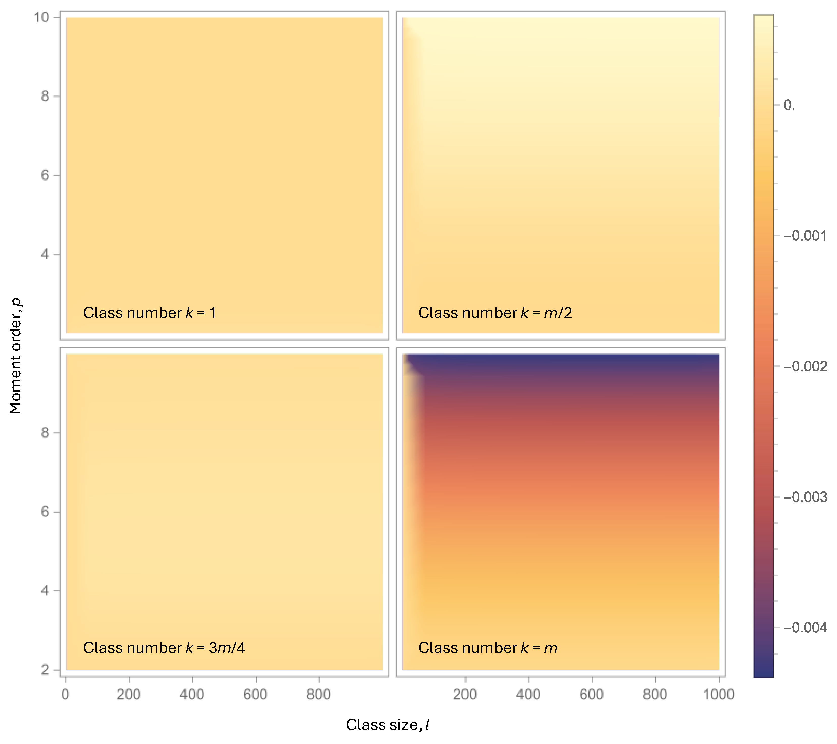
is small. An extended numerical investigation showed that this is indeed the case. An example is shown in Figure A1, where it is seen that the absolute value of the error: (a) is small, not exceeding 0.004, (b) increases with moment order, p, and class number, k, and (c) is practically independent of the class size, l. These observations allow us to locate the most extreme error as the quantity for a sufficiently high number of l. We further observe that, as , the limit of has a simple expression
which for large or small tends to zero. For , as in the applications of this study whose data are given at percentiles, and for the error is –0.0044, i.e. negligible. However, for higher values of it would become non-negligible. Therefore, it is not recommended to estimate K-moments of order higher than 10, if the data are summarized in classes.
The above analysis justifies a procedure in which the K-moments are estimated from the sample , instead of , as if each class contained just one value.
Figure A1.
Density plots of the error for a number of classes = 100 and varying moment order and class size, , and for the indicates class numbers, .
Figure A1.
Density plots of the error for a number of classes = 100 and varying moment order and class size, , and for the indicates class numbers, .
Appendix A.2. Derivations about the Lorenz Curve and the Gini Index
Given Equation (28), to find the Gini index we integrate by parts and get
and using equation (6.22) in Koutsoyiannis [10] we finally get:
The above derivation is general, based on the definition of the Lorenz curve as no specific expression or approximation of the Lorenz curve have been used.
Yet the approximation proposed in Section 3.2 is useful in several applications and can be exact in some cases as specified in Table A1. To verify the goodness of the approximation we first find the quantile function from Equation (27):
By integration we find:
which shows that the approximate expression has the same mean as the exact distribution. Furthermore:
which means that the approximate expression has the same moment as the exact distribution. In addition, by taking the LLD of with respect to , we find that
which means that the approximate expression has the same lower tail index as the exact distribution. Finally, by expressing the distribution quantile as a function of the tail function, , taking the LLD with respect to , we find that
It is noted that Equation (A10) is valid for , while for we have and, hence, in this case the approximation is not perfect in terms of the lower tail index.

Table A1.
Special cases of the ME GHL approximation.
| Case | is exact | ||
|---|---|---|---|
| General | |||
| Pareto | |||
| Pareto with shifted origin | |||
| Exponential with shifted origin | |||
| Exponential |
Appendix A.3. Maximum Entropy Distribution for Fixed Mean and Second K-Moment
The goal is to find the probability density function that maximizes the entropy
subject to the following constraints:
Total probability constraint:
Mean constraint:
constraint:
We use calculus of variations to solve the constrained optimization problem. Introducing Lagrange multipliers for the three constraints, we formulate the functional to extremize as
The maximum occurs where the functional derivative vanishes, i.e., when for all . Here, we consider a change localized at (in the form of a Dirac-like bump) and calculate the changes in the different terms. The change in the entropy term is
where only the term at point is considered from the integral, because for any . The normalization term contributes and the mean term contributes .
For the -constraint, according to the Leibniz product rule, the change has two parts:
In the first term, is treated as fixed. Since for any , the integral is:
For the second term, we observe that depends on , and so is not zero. Rather:
Hence the integral in the second term is
Consequently,
Setting yields
or
Differentiating both sides with respect to , we find:
The derivative on the right-hand side is
and so, the differential equation becomes
which is a second-order ordinary differential equation. Since , we can take its logarithm and define
and observe that the derivative of equals the left-hand side of equation (A27). We can then write it as
Taking derivatives on both sides, we find the transformed differential equation:
whose general solution is
where and are integration constants. To verify this solution, we calculate the left- and right-hand side of Equation (A30), which are, respectively,
and hence they are equal to each other. Consequently,
By integration, we find
where is a third integration constant. For , takes on the following specific values, which are used as initial conditions to find the integration constants:
If the domain of the variable is the entire real line, then we use the first two initial conditions in Equation (A35):
and, after algebraic manipulations, find
Reparametrizing by we obtain equation (37).
If the domain of the variable is the set of positive reals, then we use the last two initial conditions in Equation (A35):
and, after algebraic manipulations, find
Reparametrizing by we obtain equation (38).
As a final step, we should connect the parameters and . For the case , by integration we find the mean, , and the K-momentas
and hence, by solving the system of two equations, the final results are
For the latter case the respective equations do not have an analytical solution, and a numerical procedure is needed to find the parameters and from and . All required equations, obtained through integration using the definitions of the different quantities, are gathered in Table 1. Alternatively, the approximate equations (39) and (40) can be used for direct calculations of all required quantities.
Appendix A.4. Assignment of Distribution Function Values for the Observed Sample Values
Assuming that the observed sample is given as a sequence of values representative for consecutive percentiles , it is reasonable to assume that the value corresponds to a value of the distribution function = 0.01/2 = 0.005, the value corresponds to = (0.01 + 0.02) / 2 = 0.015, and so on, up to the value that corresponds to = (0.98 + 0.99) / 2 = 0.985. However, this simple technique is not reliable for the last point , while the estimation of is crucial for determining the upper tail of the distribution. Here, we follow a more reliable procedure.
At a first step we estimate the upper tail index as the regression slope of vs. (where is the value of the odds function) for the highest few (say, 5-6) points , excluding the point , as at this phase is unknown. (Likewise, we estimate the lower tail index , but by using the lowest few points .) Then we assume that a Pareto tail applies beyond , i.e.,
The mean value beyond is
and the required value of the distribution function at is
where in our case . For the limiting expression has the form
Appendix A.5. Calculation of Empirical Entropy
For each of the first 99 percentiles we estimate the , where in our case = 0.01. The contribution of each to entropy is then . However, according to the Pareto tail assumed in Appendix A.4., the contribution of the last percentile is
where, for the Pareto tail after algebraic manipulations, we have
and hence
where in our case and .
References
- Aριστοτέλους, Hθικά Νικομάχεια (Aristotle, Nicomachean Ethics, 1107a.1). https://www.mikrosapoplous.gr/aristotle/nicom2b.htm.
- Koutsoyiannis, D.; Sargentis, G.-F. Entropy and wealth, Entropy 2021, 23 (10), 1356. [CrossRef]
- Jaynes, E.T. Information theory and statistical mechanics. Physical Review 1957, 106(4), 620-630. [CrossRef]
- UNU-WIDER, World Income Inequality Database (WIID) Companion dataset (wiidcountry), Version 29 April 2025. https://doi.org/10.35188/UNUWIDER/WIIDcomp-290425.
- World Income Inequality Database (WIID), WIID Companion User Guide, Available online: https://www.wider.unu.edu/sites/default/files/WIID/WIID-Companion-User-Guide-29April2025.pdf (accessed on 1 November 2025).
- Shannon, C.E. The mathematical theory of communication. Bell System Technical Journal 1948, 27 (3), 379-423. [CrossRef]
- Jaynes, E.T., 2003. Probability Theory: The Logic of Science, Cambridge Univ. Press, Cambridge, UK, 728 pp.
- Uffink, J. Can the maximum entropy principle be explained as a consistency requirement? Studies In History and Philosophy of Modern Physics 1995, 26 (3), 223-261. [CrossRef]
- Sargentis, G.-F.; Iliopoulou, T.; Dimitriadis, P.; Mamassis, N.; Koutsoyiannis, D. Stratification: An Entropic View of Society’s Structure. World 2021, 2, 153-174. [CrossRef]
- Koutsoyiannis, D. Stochastics of Hydroclimatic Extremes - A Cool Look at Risk, Edition 4, 400 pages, Kallipos, Athens, Greece, 2024, ISBN: 978-618-85370-0-2, 333 pp. https://www.itia.ntua.gr/2000/ (accessed on 1 August 2021).
- Marx, K.; Engels, F. The German Ideology; International Publishers: New York, NY, USA, 1970; Volume 1, Available online: https://archive.org/details/germanideology00marx/ (accessed on 1 November 2025).
- World Inequality Report 2022 - Executive Summary. Available online: https://wir2022.wid.world/executive-summary/.
- Global Inequalities – IMF. Available online: https://www.imf.org/en/Publications/fandd/issues/2022/03/Global-inequalities-Stanley (accessed on 1 November 2025).
- 2022 Income Inequality Decreased for First Time Since 2007 – Census.gov, Available online: https://www.census.gov/library/stories/2023/09/income-inequality.html (accessed on 1 November 2025).
- Income and Wealth Inequality in America, 1949-2016 – Federal Reserve Bank of Minneapolis. Available online: https://www.minneapolisfed.org/research/institute-working-papers/income-and-wealth-inequality-in-america-1949-2016 (accessed on 1 November 2025).
- Inequality in China: The Basics. Available online: https://www.csis.org/analysis/how-inequality-undermining-chinas-prosperity#h2-inequality-in-china-the-basics (accessed on 1 November 2025).
- Xi Jinping: We must adhere to the people-centred development philosophy. Friends of Socialist China. Available online: https://socialistchina.org/2025/05/02/xi-jinping-we-must-adhere-to-the-people-centred-development-philosophy/ (accessed on 1 November 2025).
- India ranks 4th globally in income equality, shows World Bank data. Available online: https://timesofindia.indiatimes.com/india/india-ranks-4th-globally-in-income-equality-shows-world-bank-data/articleshow/122272852.cms (accessed on 1 November 2025).
- What is the state of inequality in India? - The Hindu. Available online: https://www.thehindu.com/business/Economy/what-is-the-state-of-inequality-in-india/article69805101.ece (accessed on 1 November 2025).
- Living conditions in Europe - income distribution and income inequality – Eurostat. Available online: https://ec.europa.eu/eurostat/statistics-explained/index.php/Living_conditions_in_Europe_-_income_distribution_and_income_inequality (accessed on 1 November 2025).
- Russia Economic Report – World Bank. Available online: https://www.worldbank.org/en/country/russia/publication/rer (accessed on 1 November 2025).
- GDP per capita (current US$) – China, India, United States, Russian Federation, European Union. Available online: https://data.worldbank.org/indicator/NY.GDP.PCAP.CD?end=2024&locations=CN-IN-US-RU-EU&start=1960&view=chart (accessed on 1 November 2025).
- GDP per capita, PPP (current international $) – China, India, United States, Russian Federation, European Union. Available online: https://data.worldbank.org/indicator/NY.GDP.PCAP.PP.CD?end=2024&locations=CN-IN-US-RU-EU&start=1960&view=chart (accessed on 1 November 2025).
- Lewis, D.K. The History of Argentina. Bloomsbury Publishing USA, 2014.
- Argentina After World War II: From Peronism to Dictatorship. Available online: https://oercommons.org/courseware/lesson/88088/student-old/?task=2 (accessed on 1 November 2025).
- Little, W. Party and State in Peronist Argentina, 1945-1955. Hispanic American Historical Review 1973; 53 (4), 644–662. [CrossRef]
- Katie A. Dirty War Argentina [1976–1983]. Britannica. Available online: https://www.britannica.com/event/Dirty-War-Argentina (accessed on 1 November 2025).
- Pion-Berlin, D. Argentina: The Journey from Military Intervention to Subordination. Oxford Research Encyclopedia of Politics, 2020. [CrossRef]
- Romero, L.A. A History of Argentina in the Twentieth Century: Updated and revised edition. Penn State Press, 2013.
- Spruk, R. The rise and fall of Argentina. Lat Am Econ Rev 2019, 28, 16. [CrossRef]
- Ferre JC. The Rise of Javier Milei and the Emergence of Authoritarian Liberalism in Argentina. Latin American Research Review, 2025, 1-12. [CrossRef]
- Civilian casualties after the air attack and massacre on Plaza de Mayo, June 1955. Available online: https://en.wikipedia.org/wiki/Revoluci%C3%B3n_Libertadora#/media/File:Plaza-Mayo-bombardeo-1955.JPG (accessed on 1 November 2025).
- Cordobazo. General strike in protest against the political and economic decisions of the military dictatorship. Bulevar San Juan, Córdoba Capital. In that place was murdered that day, the SMATA worker Máximo Mena. Available online: https://en.wikipedia.org/wiki/Cordobazo#/media/File:Cordobazo.jpg (accessed on 1 November 2025).
- Fernando Luiz L.; Koury A.P. In the beginning, there was land. Street Matters: A Critical History of Twentieth-Century Urban Policy in Brazil. University of Pittsburgh Press, 2022, pp. 19–36. [CrossRef]
- Carter M. Social Inequality, Agrarian Reform, and Democracy in Brazil. Available online: https://static1.squarespace.com/static/5bbd787251f4d47ff1881d9b/t/5cdc38b4a4222fbfda5e7e86/ (accessed on 1 November 2025).
- Fischer, B. (, June 25). Favelas and Politics in Brazil, 1890–1960. Oxford Research Encyclopedia of Latin American History, 2019. [CrossRef]
- Brazil profile – Timeline. BBC, 3 January 2019. Available online: https://www.bbc.com/news/world-latin-america-19359111 (accessed on 1 November 2025).
- Panoramic view of Rio's Rocinha favela. Available online: https://en.wikipedia.org/wiki/Favela#/media/File:1_rocinha_panorama_2014.jpg (accessed on 1 November 2025).
- Library of Congress. Brazil-US Relations. Military Dictatorship (1964-1985). Available online: https://guides.loc.gov/brazil-us-relations/military-dictatorship (accessed on 1 November 2025).
- Talarico A. Deeply Divided Brazil. Available online: https://www.beyondintractability.org/casestudy/deeply-divided-brazil (accessed on 1 November 2025).
- Klein H.S.; Vidal Luna F. Brazil. An Economic and Social History from Early Man to the 21st Century. Cambridge University Press. [CrossRef]
- Michener G.; Pereira C. A Great Leap Forward for Democracy and the Rule of Law? Brazil’s Mensalão Trial. Journal of Latin American Studies 2016, 48(3):477-507. [CrossRef]
- The Editors of Encyclopaedia Britannica. “apartheid”. Encyclopedia Britannica, 17 Sep. 2025, Available online: https://www.britannica.com/topic/apartheid (accessed on 25 October 2025).
- South African History Online. (2016, May 6). A history of Apartheid in South Africa. South African History Online. Available online: https://sahistory.org.za/article/history-apartheid-south-africa (accessed on 1 November 2025).
- Larson Z. South Africa: Twenty-Five Years Since Apartheid. Origins. Current Events in Historical Perspective. Available online: https://origins.osu.edu/article/south-africa-mandela-apartheid-ramaphosa-zuma-corruption (accessed on 1 November 2025).
- Mandela, N. Long walk to freedom: The autobiography of Nelson Mandela. Hachette UK, 2008. Preview available online: https://books.google.gr/books?hl=en&lr=&id=jc41AQAAQBAJ&oi=fnd&pg (accessed on 1 November 2025).
- Netshitenzhe, J. Inequality matters: South African trends and interventions. New Agenda: South African Journal of Social and Economic Policy 2014, 53. Available online: https://www.ajol.info/index.php/na/article/view/111806/101572 (accessed on 1 November 2025).
- Lawal S. South Africa: 30 years after apartheid, what has changed? Al Jazeera 27 Apr 2024. Available online: https://www.aljazeera.com/news/2024/4/27/south-africa-30-years-after-apartheid-what-has-changed (accessed on 1 November 2025).
- Makgetla N. Inequality in South Africa: An overview. September 2020. Available online: https://tips.org.za/images/TIPS_Working_Paper_Inequality_in_South_Africa_An_Overview_September_2020.pdf (accessed on 1 November 2025).
- United Nations. Corruption & Economic Crime. Available online: https://dataunodc.un.org/dp-crime-corruption-offences (accessed on 1 November 2025).
- World Bank Group. International Homicides (per 100,000 people) – South Africa. Available online: https://data.worldbank.org/indicator/VC.IHR.PSRC.P5?locations=ZA (accessed on 1 November 2025).
- United Nations. International homicide. Available online: https://dataunodc.un.org/dp-intentional-homicide-victims (accessed on 1 November 2025).
- Global Organized Crime Index. Available online: https://ocindex.net/country/south_africa (accessed on 1 November 2025).
- Bulgaria country profile. BBC. Available online: https://www.bbc.com/news/world-europe-17202996 (accessed on 1 November 2025).
- The History of Communism in Bulgaria. Available online: https://openendedsocialstudies.org/2018/01/11/the-history-of-communism-in-bulgaria/ (accessed on 1 November 2025).
- Todorov A. The state of the right: Bulgaria. Fondation pour l’innovation politique (Fondapol). Available online: https://www.fondapol.org/en/study/the-state-of-the-right-bulgaria/ (accessed on 1 November 2025).
- Zmigrodzki, M. Issues facing the transformation of the political system in Bulgaria, Global Economic Review 1992, 21 (1), 95-108. [CrossRef]
- Hill, R.J.; White, S. Referendums in Russia, the Former Soviet Union and Eastern Europe. In: Qvortrup, M. (ed.) Referendums Around the World. Palgrave Macmillan, London2014. [CrossRef]
- Apartment block in district of Sveta Troitsa, Sofia, Bulgaria. Available online: https://commons.wikimedia.org/wiki/File:Apartment_block_in_district_of_Sveta_Troitsa,_Sofia,_Bulgaria.jpg (accessed on 1 November 2025).
Figure 1.
Visual comparison of the exact Lorenz curves for the PBF distribution function with four different parameters sets (shown in each of the four panels) with the approximation of Equation (30). Except for the Pareto case, the parameter was determined so as to maximize entropy for a chosen parameter.
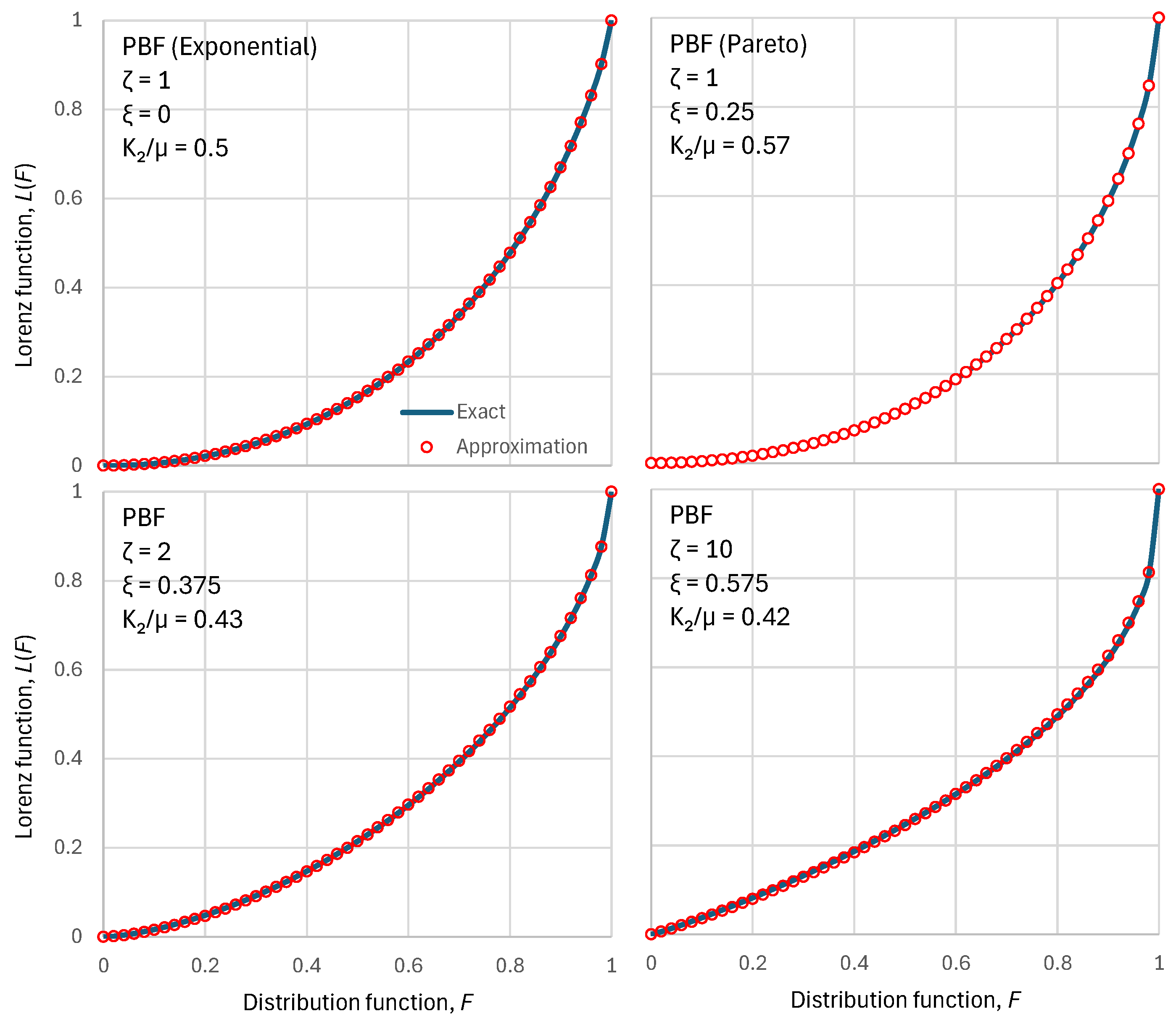
Figure 2.
Visual comparison of the exact Lorenz curves for the Dagum distribution function with four different parameters sets (shown in each of the four panels) with the approximation of Equation (30). Except for the upper-left case, the parameter was determined so as to maximize entropy for a chosen parameter.
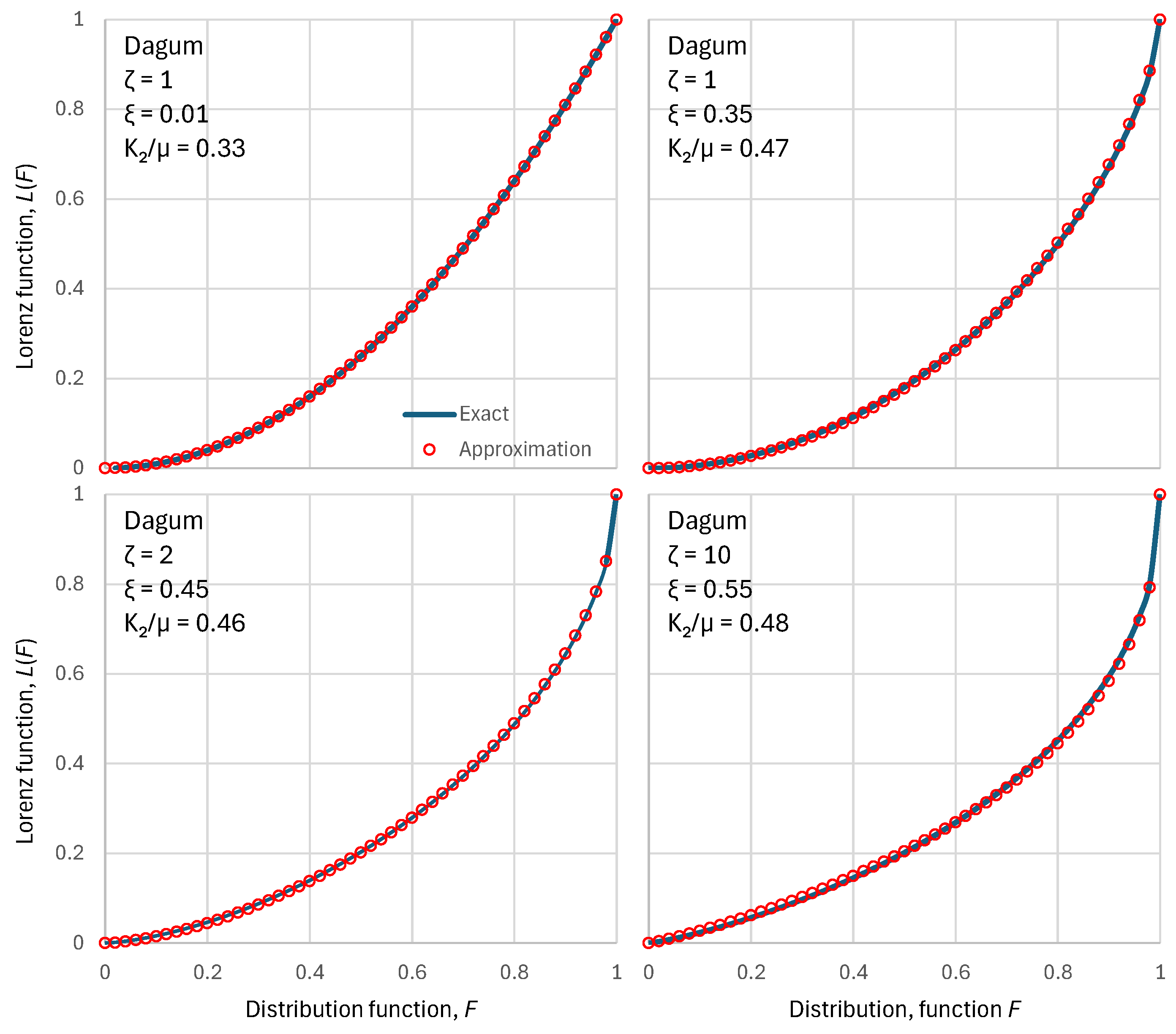
Figure 3.
Visual comparison of statistical characteristics of two distribution functions, PBF and Dagum with parameters as shown in the legend, having the same K-spread coefficient (Gini index), , and different standardized entropies 0.88 and 0.97, respectively. (upper left) Lorenz curves, which are very similar for the two distributions; (upper right) distribution functions plotted in the form of the variable vs. the odds function , which shows the substantially different behaviour of the distributions, especially in the tails; (lower) probability density function on (left) linear and (right) logarithmic plots.
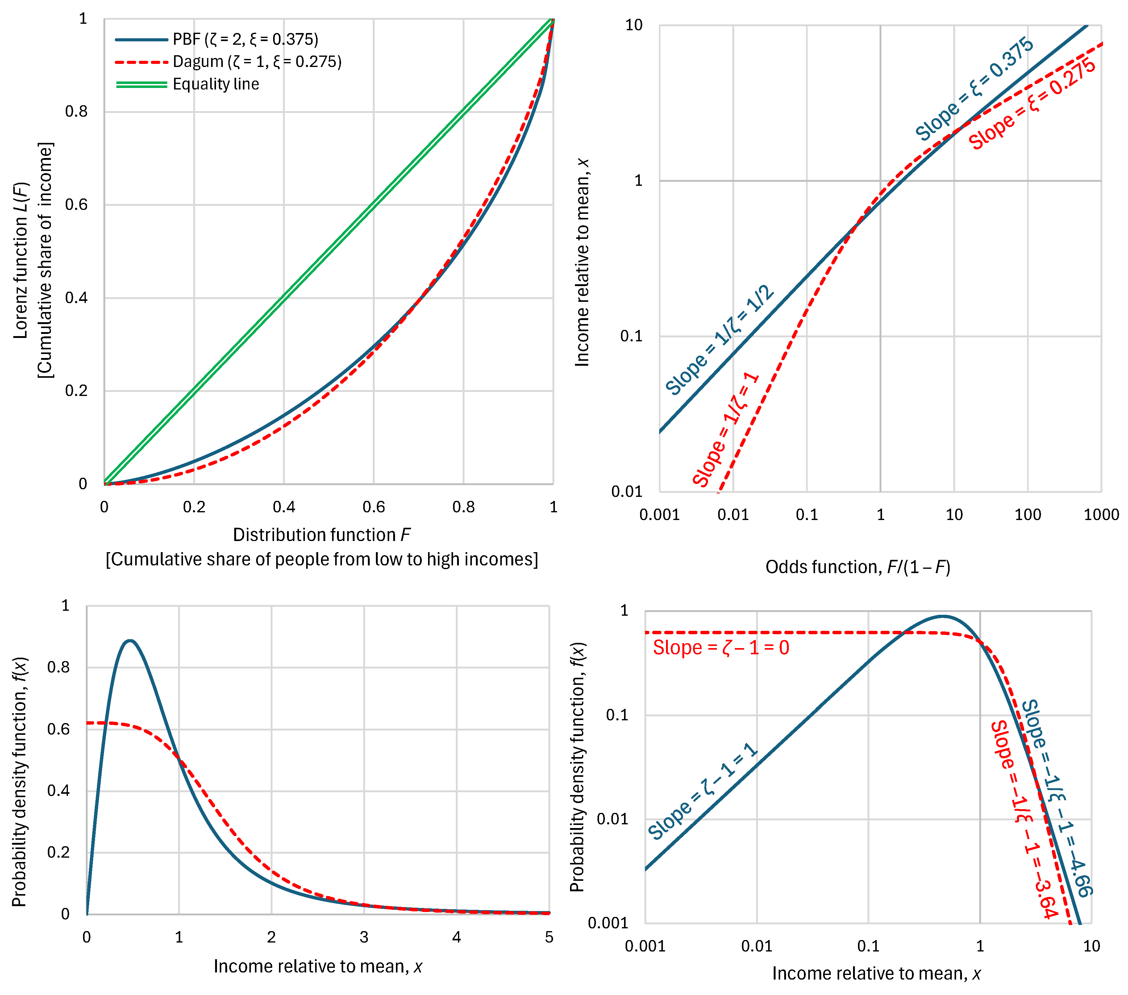
Figure 4.
Detailed graphs of economic indicators of Bulgaria in 1971 (clockwise from upper left): Lorenz curve; odds function; probability density function; and graph of K-centre and K-spread vs. K-moment order, where for reference the theoretical curves of the ME exponential distribution are also plotted in dotted lines.
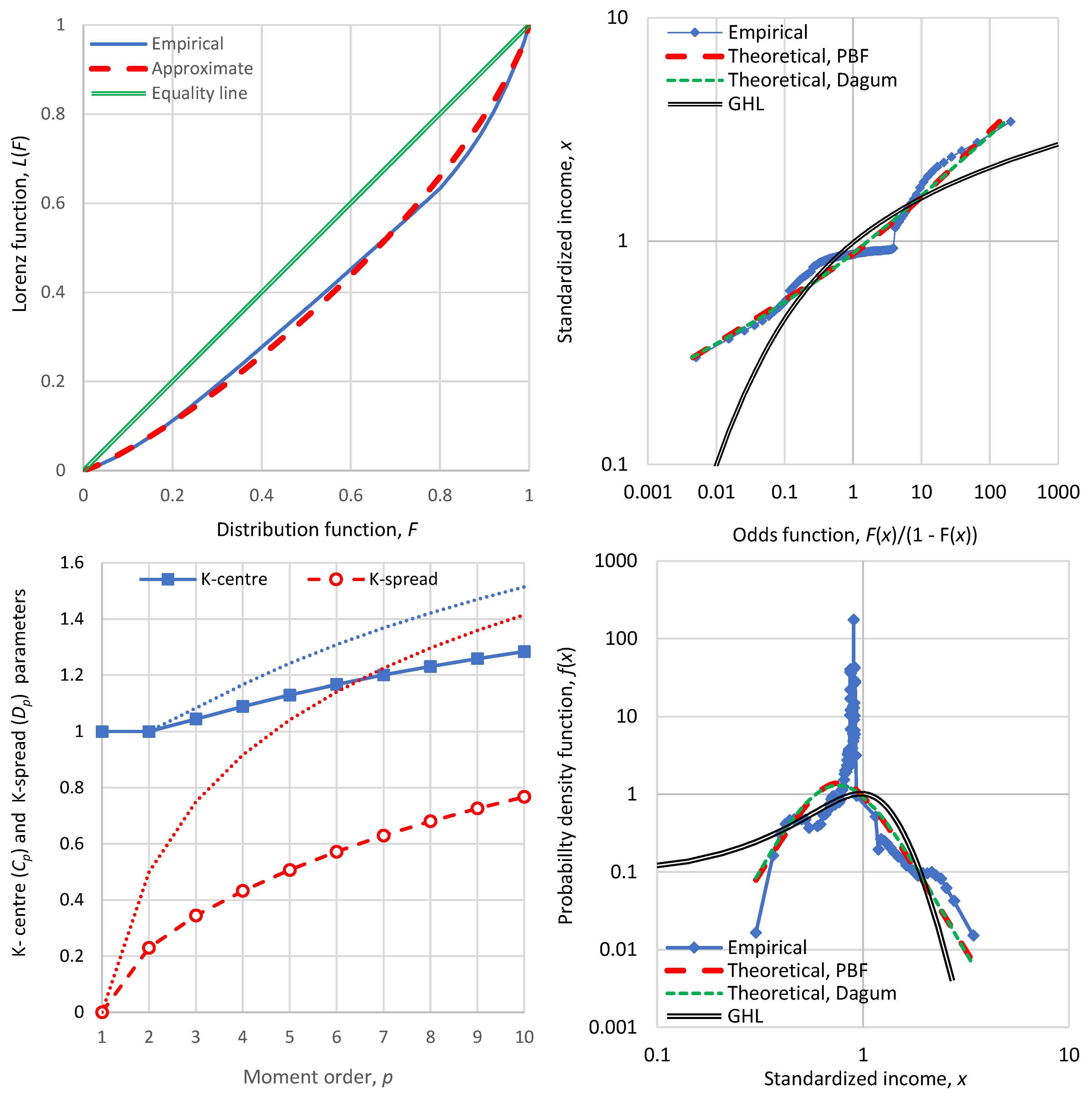
Figure 5.
Visualization of the behaviour of the bounded exponential distribution, resulting from maximization of entropy for fixed mean and upper bound : (left) two instances of the probability density function for the indicated values of the upper bound and for scale parameter ; (right) variation of standardized mean, K-spread coefficient (Gini index) and standardized entropy, for varying upper bound .
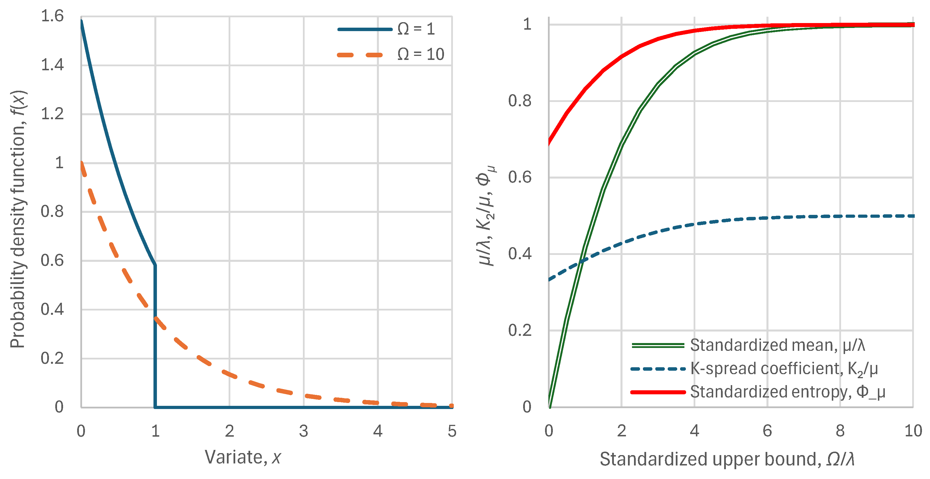
Figure 6.
Maximum entropy vs. K-spread curve: Maximum standardized entropy that is feasible for a specified K-spread coefficient (Gini index). A particular state, defined as a point () is feasible only if it lies below this curve. The exact curve corresponds to the generalized half logistic (GHL) distribution, while different approximations (practically indistinguishable from the exact curve) are also plotted.
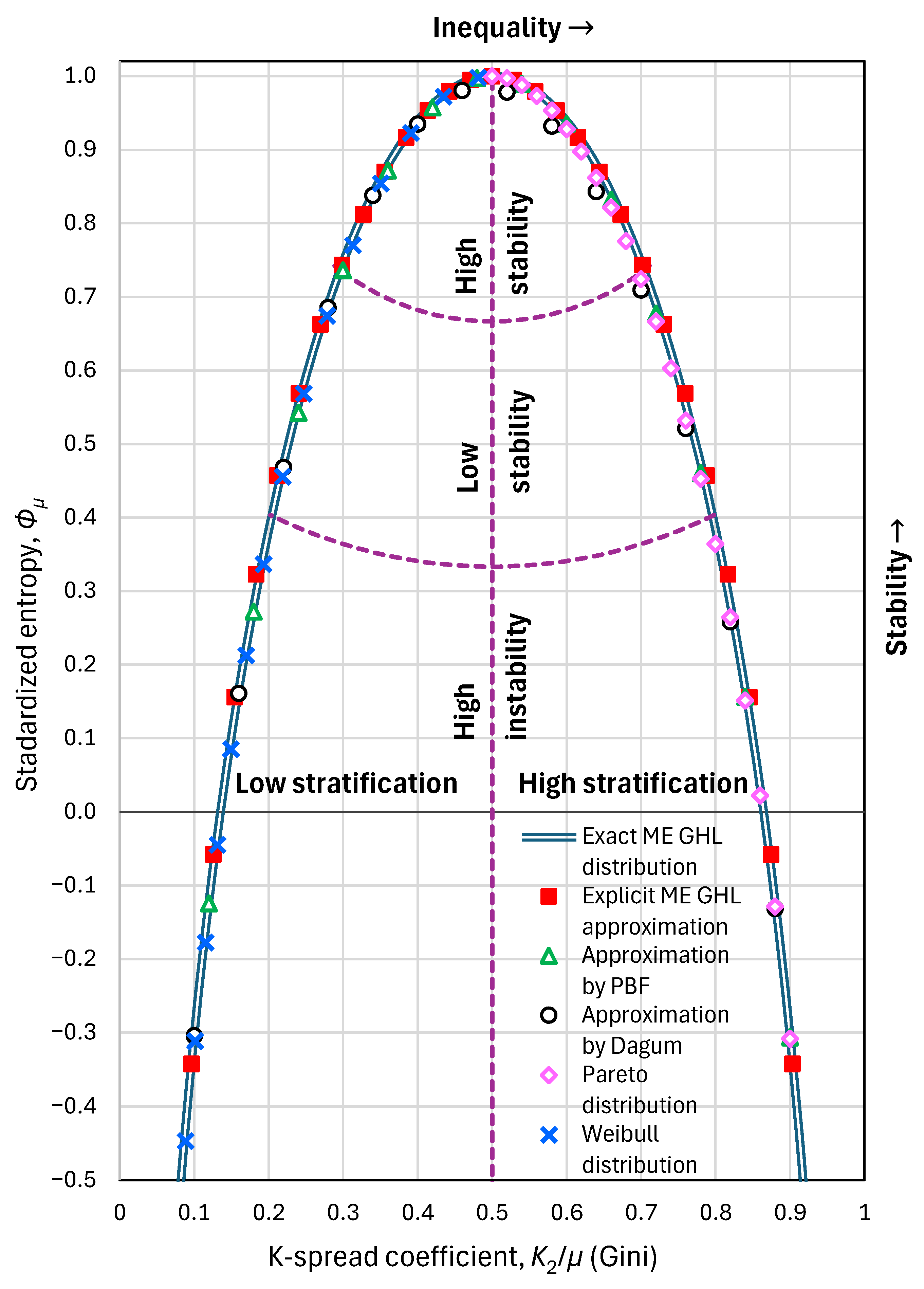
Figure 7.
Approximations of the maximum entropy vs. K-spread curve: (left) approximation errors, defined as differences of the standardized entropy derived from approximations minus the exact values of the ME GHL distribution; (right) tail indices of the approximating distributions.
Figure 7.
Approximations of the maximum entropy vs. K-spread curve: (left) approximation errors, defined as differences of the standardized entropy derived from approximations minus the exact values of the ME GHL distribution; (right) tail indices of the approximating distributions.
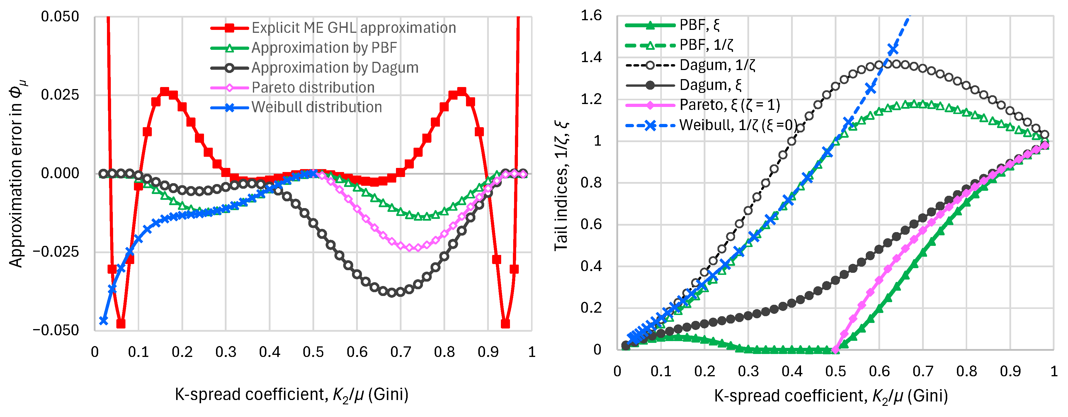
Figure 8.
Detailed graphs of economic indicators of USA in 2022 (clockwise from upper left): Lorenz curve; odds function; probability density function; and graph of K-centre and K-spread vs. K-moment order, where for reference the theoretical curves of the ME exponential distribution are also plotted in dotted lines.
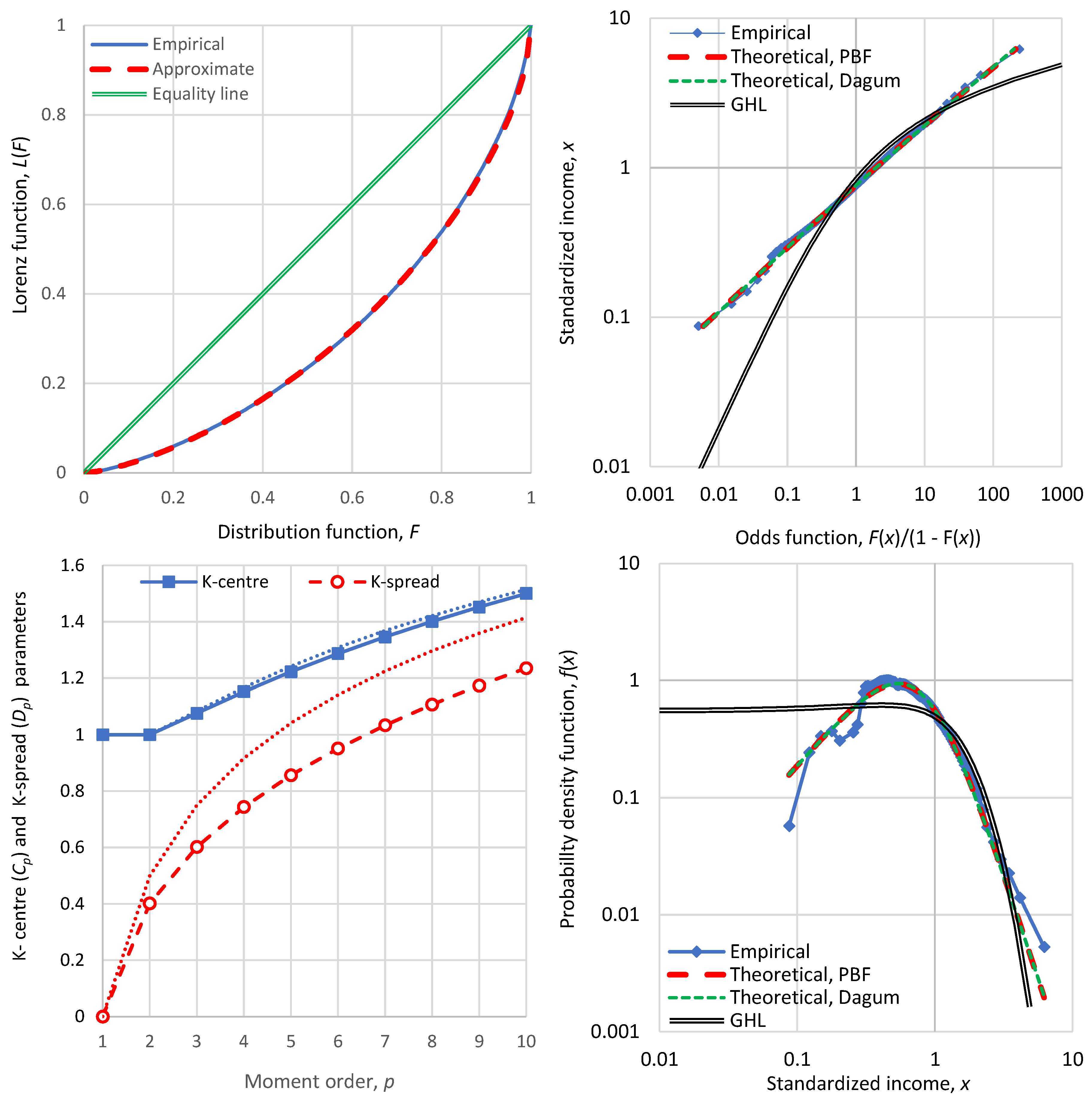
Figure 9.
Detailed graphs of economic indicators of China in 2022 (clockwise from upper left): Lorenz curve; odds function; probability density function; and graph of K-centre and K-spread vs. K-moment order, where for reference the theoretical curves of the ME exponential distribution are also plotted in dotted lines.
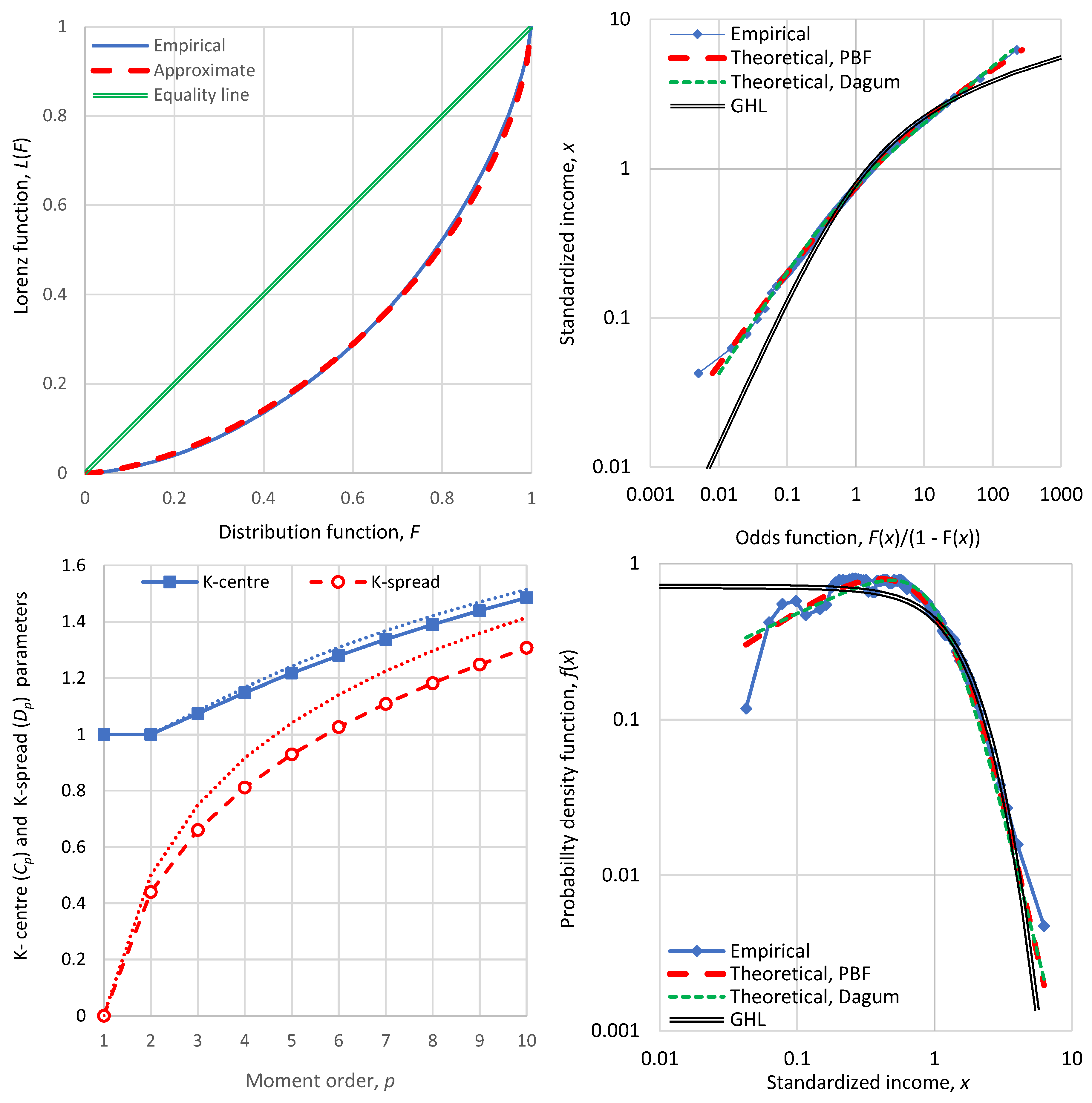
Figure 10.
Characteristic graphs for the examined five major geopolitical players in 2022 (clockwise from upper left): standardized entropy vs. K-spread coefficient (Gini index), plotted alongside the maximum entropy vs. K-spread curve; distance from the pole of maximum entropy; GDP per capita [22]; GDP-PPP per capita, [23].
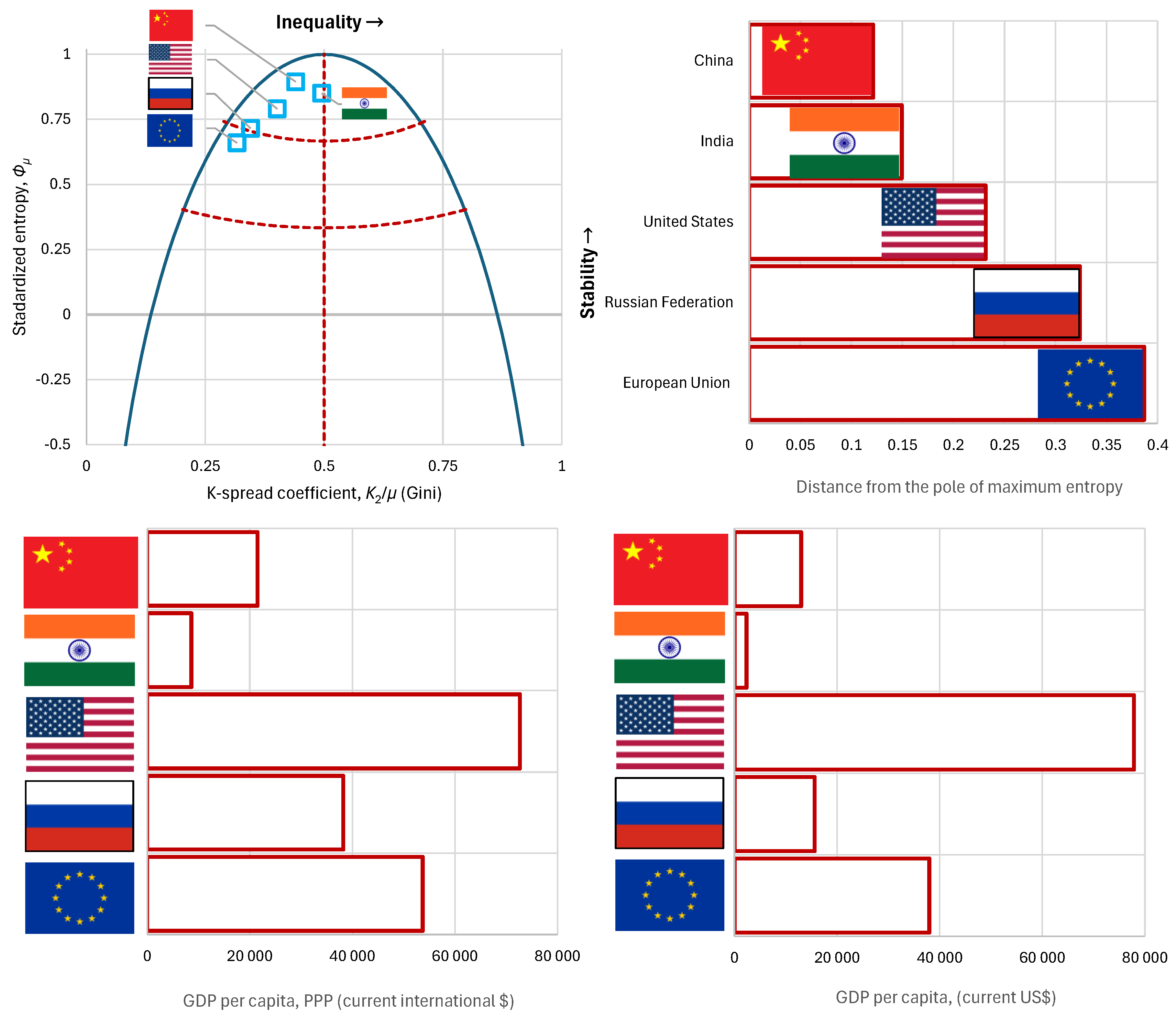
Figure 11.
Characteristic violent events in Argentina in the 20th century: (left) civilian casualties after the air attack and massacre on Plaza de Mayo, June 1955 [32]; (right) Cordobazo general strike in protest against the political and economic decisions of the military dictatorship, Bulevar San Juan, Córdoba Capital, May 1969 [33].
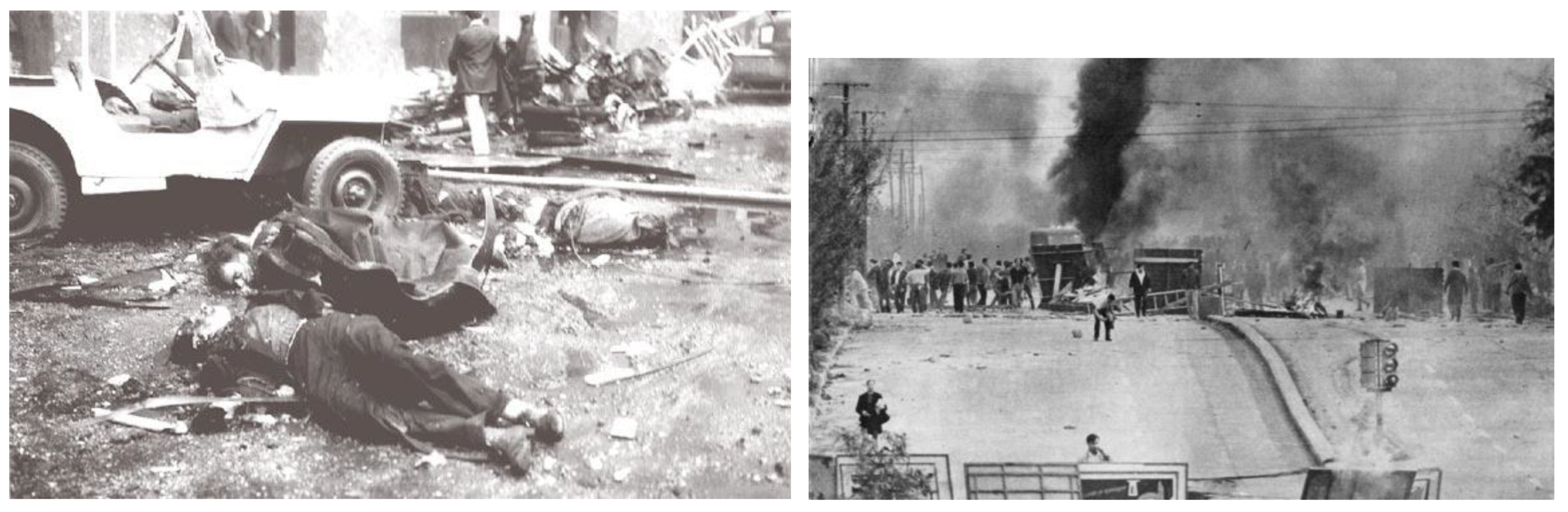
Figure 12.
Characteristic graphs for the evolution of major economic indices in Argentina: (left): standardized entropy vs. K-spread coefficient (Gini index), plotted alongside the maximum entropy vs. K-spread curve; (right) distance from the pole of maximum entropy with the grey lines indicating the times of coups d’état.
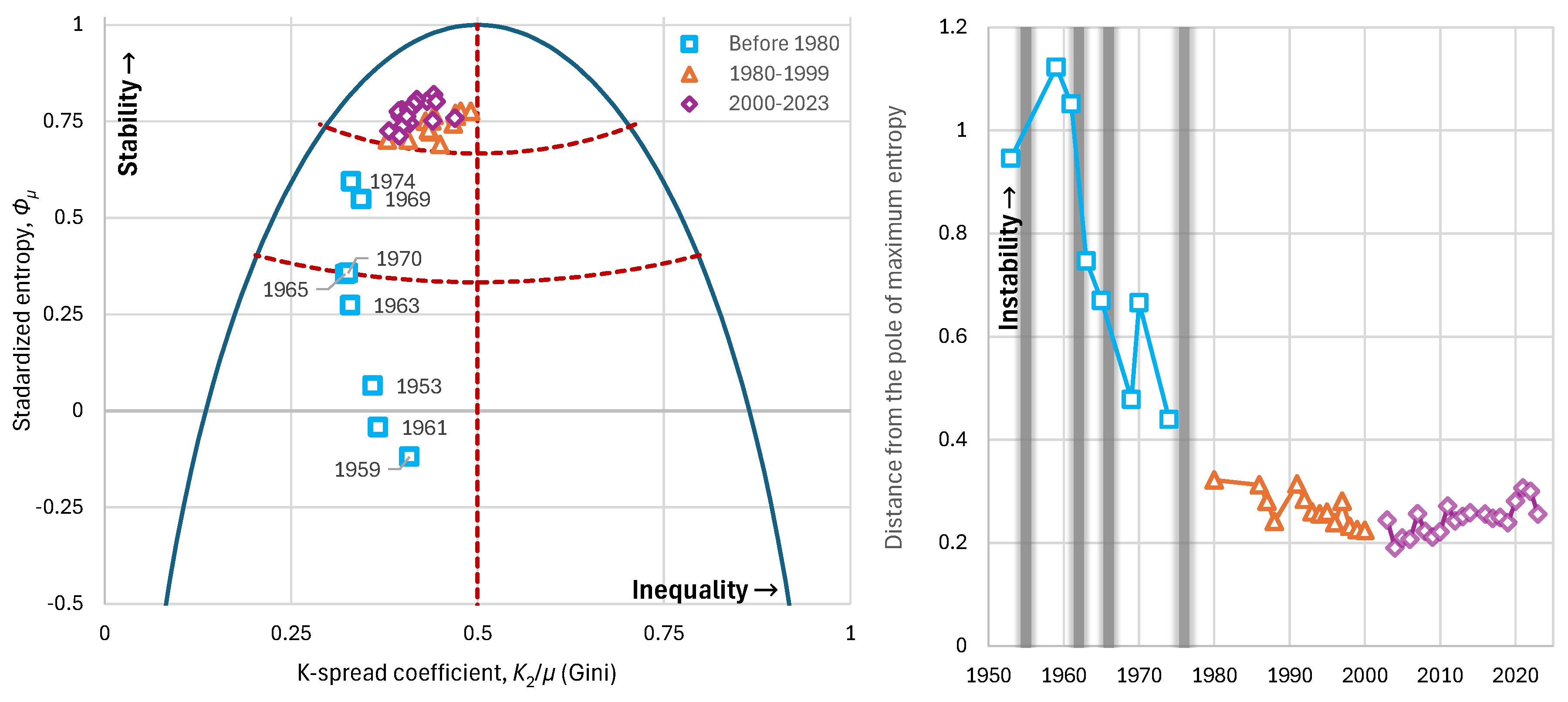
Figure 13.
Panoramic view of Rio’s Rocinha favela, contrasted by high-rise buildings (condominiums) near the coast (of South Atlantic Ocean) in São Conrado [38].
Figure 13.
Panoramic view of Rio’s Rocinha favela, contrasted by high-rise buildings (condominiums) near the coast (of South Atlantic Ocean) in São Conrado [38].
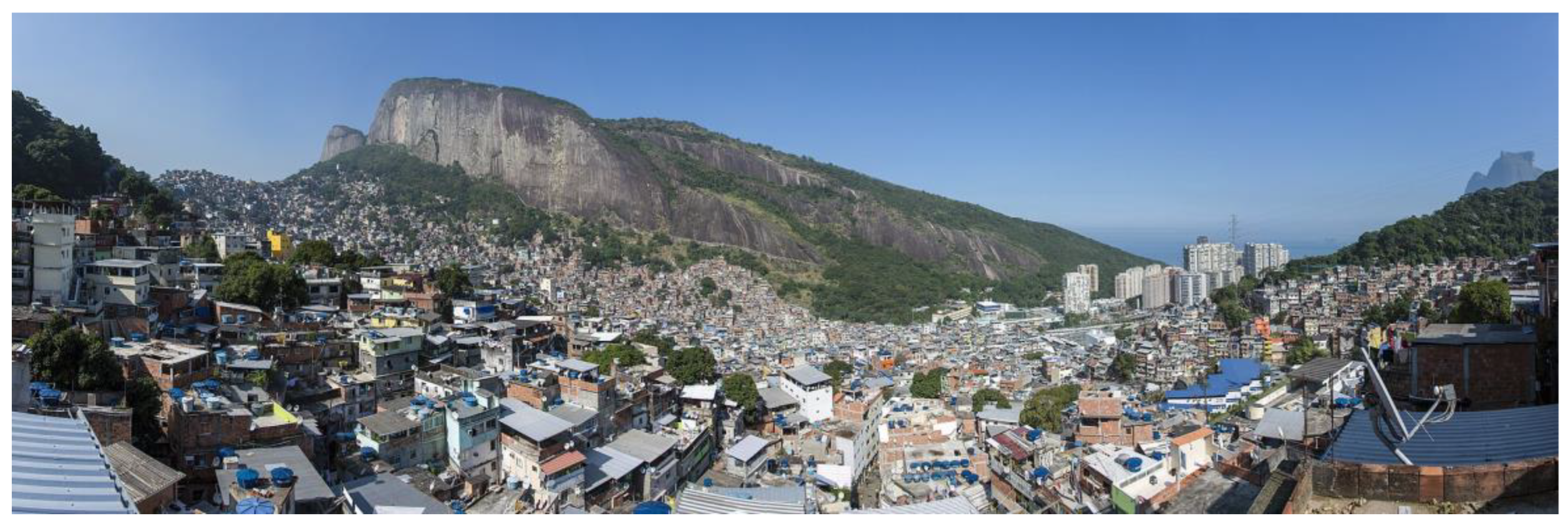
Figure 14.
Characteristic graphs for the evolution of major economic indices in Brazil: (left): standardized entropy vs. K-spread coefficient (Gini index), plotted alongside the maximum entropy vs. K-spread curve; (right) distance from the pole of maximum entropy.
Figure 14.
Characteristic graphs for the evolution of major economic indices in Brazil: (left): standardized entropy vs. K-spread coefficient (Gini index), plotted alongside the maximum entropy vs. K-spread curve; (right) distance from the pole of maximum entropy.
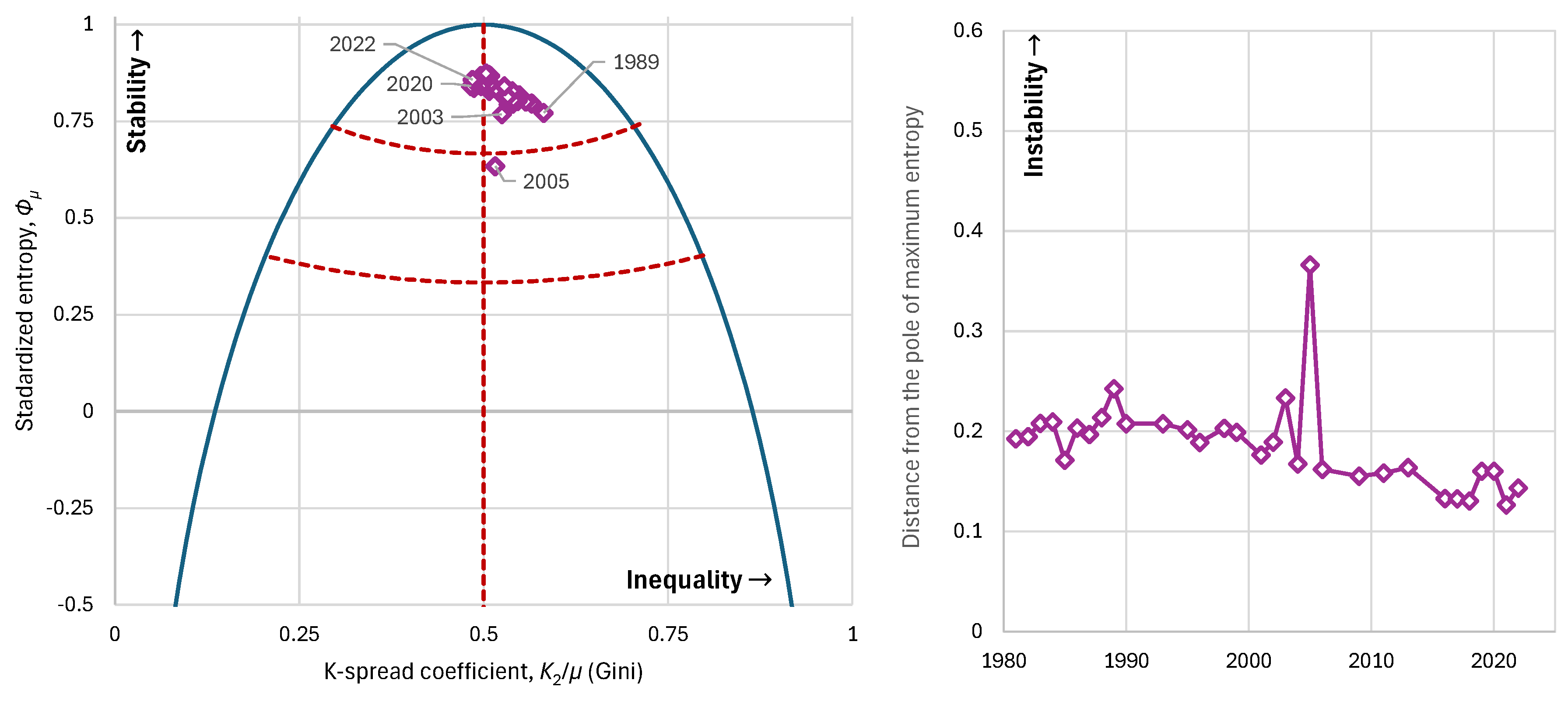
Figure 15.
Characteristic graphs for the evolution of major economic indices in South Africa: (left): standardized entropy vs. K-spread coefficient (Gini index), plotted alongside the maximum entropy vs. K-spread curve; (right) distance from the pole of maximum entropy.
Figure 15.
Characteristic graphs for the evolution of major economic indices in South Africa: (left): standardized entropy vs. K-spread coefficient (Gini index), plotted alongside the maximum entropy vs. K-spread curve; (right) distance from the pole of maximum entropy.
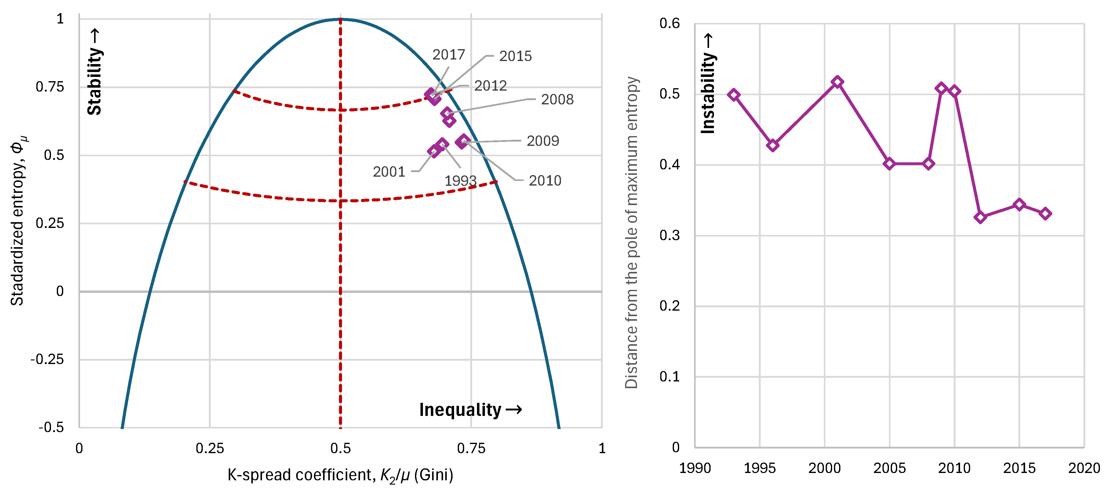
Figure 16.
Apartment blocks in Sveta Troitsa, Sofia, Bulgaria, at the northwest end of the district, next to a train station [59].
Figure 16.
Apartment blocks in Sveta Troitsa, Sofia, Bulgaria, at the northwest end of the district, next to a train station [59].

Figure 17.
Characteristic graphs for the evolution of major economic indices in Bulgaria: (left): standardized entropy vs. K-spread coefficient (Gini index), plotted alongside the maximum entropy vs. K-spread curve; (right) distance from the pole of maximum entropy. The cyan rectangles represent the era of Soviet influence and the purple diamonds the era of free market.
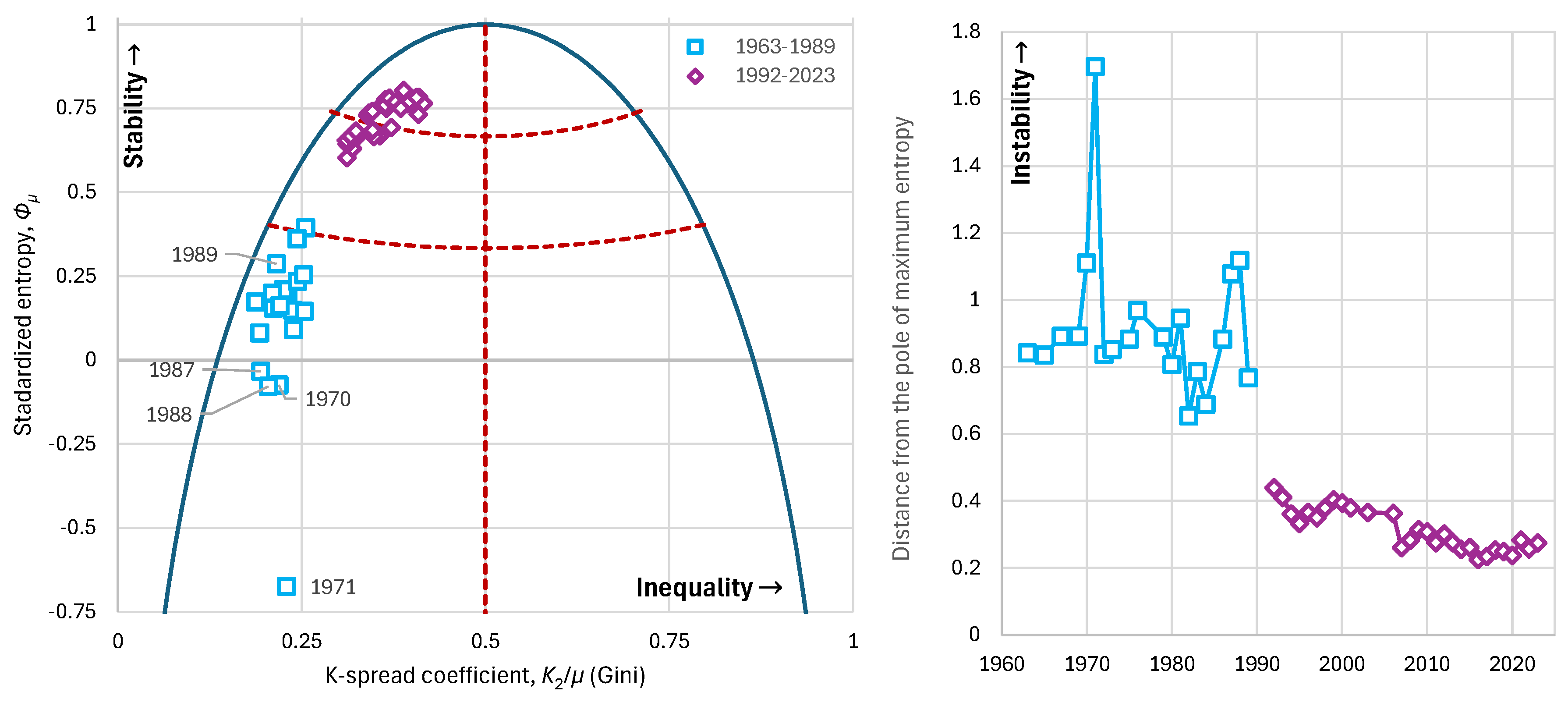
Table 1.
Distribution functions used in the study and their main characteristics.*
| Exponential, |
|||||
| Bounded exponential, |
|
||||
| Logistic, |
|||||
| GHL, |
|
||||
| Pareto (), |
|
||||
| Weibull (), |
|||||
| PBF, |
As |
|
|||
| Dagum, |
|
As |
|
* Clarifications of symbols: is the Euler’s constant; and
are the gamma and beta functions;is the digamma function; is the pth harmonic number; is a scale parameter; and are the upper and lower tail indices,respectively; is a shape parameter. The support of the bounded exponential distribution is . The support of the logistic distribution is and its upper and lower tail indices are . For all other distributions, the support is and the upper and lower tail indices are , respectively; when expressions do not include either of the two, their values are , . Note that for the PBF and Dagum distributions become identical.
Table 2.
Characteristic indices for the economies of the major geopolitical powers in 2022 .
| Country, year | ||||||
|---|---|---|---|---|---|---|
| China, 2022 | 0.44 | 0.89 | 0.12 | 2.97 | 0.34 | 1.98 |
| India, 2022 | 0.49 | 0.89 | 0.15 | 3.13 | 0.50 | 1.02 |
| USA, 2022 | 0.40 | 0.79 | 0.23 | 3.08 | 0.41 | 2.31 |
| Russian Federation, 2022 | 0.35 | 0.72 | 0.32 | 2.97 | 0.31 | 3.48 |
| European Union, 2022 | 0.32 | 0.66 | 0.39 | 3.02 | 0.34 | 1.68 |
| Bulgaria, 1971 | 0.23 | – 0.67 | 1.69 | 3.34 | 0.20 | 5.84 |
Note: Bulgaria (1971), also shown in Figure 4, was included as an extreme case for comparison. The lowest or highest values of the indices that favour equality or stability are highlighted in bold; namely equality is manifested by low and high , while stability is reflected in high and low .
Disclaimer/Publisher’s Note: The statements, opinions and data contained in all publications are solely those of the individual author(s) and contributor(s) and not of MDPI and/or the editor(s). MDPI and/or the editor(s) disclaim responsibility for any injury to people or property resulting from any ideas, methods, instructions or products referred to in the content. |
© 2025 by the authors. Licensee MDPI, Basel, Switzerland. This article is an open access article distributed under the terms and conditions of the Creative Commons Attribution (CC BY) license (http://creativecommons.org/licenses/by/4.0/).
Copyright: This open access article is published under a Creative Commons CC BY 4.0 license, which permit the free download, distribution, and reuse, provided that the author and preprint are cited in any reuse.


