
Submitted:
29 October 2025
Posted:
30 October 2025
You are already at the latest version
Abstract
A person's face can reveal their mood, and microexpressions, although brief and involuntary, are also authentic. People can recognize facial gestures; however, their accuracy is inconsistent, highlighting the importance of objective computational models. Various artificial intelligence models have classified microexpressions into three categories: positive, negative, and surprise. However, it is still significant to address the basic Ekman microexpressions (joy, sadness, fear, disgust, anger, and surprise). This study proposes a Transformers-based machine learning model, trained on CASME, SAMM, SMIC, and its own datasets. The model offers comparable results with other studies when working with seven classes. It applies various component-based techniques ranging from ViT to optical flow with a different perspective, with low training rates and competitive metrics comparable with other publications on a laptop. These results can serve as a basis for future research.
Keywords:
facial microexpressions
; transformers vision
; multi-head attention
; facial recognition
1. Introduction
Facial expressions appear daily in human beings. They involve changes in the face that reflect emotional states; however, individuals may conceal or disguise their true feelings [1]. Despite this, the production of micro-expressions is unavoidable, as they tend to occur involuntarily within a second fraction, often becoming imperceptible to the human eye [2].
The recognition of micro-expressions is a research topic with various fields of practical application, such as in [3], where it is employed to identify emotions from a psychological perspective. There are basic emotions: happiness, surprise, contempt, sadness, anger, disgust, and fear, which can be used to analyze an individual’s emotional behavior in order to assess their actual emotional state [3]. Throughout this work, the focus will be placed on the basic emotions identified by Ekman [4,5,6].
Various techniques have been used for their analysis. For example, in [7], mathematical strategies are employed to address the recognition of micro-expressions and the micro-movements involved; in [8], image analysis is conducted across different domains, providing a comparison of the obtained results; and in [9], the Extreme Learning Machine technique is implemented for the recognition of seven types of basic expressions.
In recent years, one of the technologies with the greatest growth due to its versatility and adaptability has been neural networks. In several of the consulted works, such as [2,7,8], and [9], some variation of this technology is applied to solve problems related to facial analysis. Throughout this project, a solution for the detection of facial micro-expressions based on neural networks is presented.
1.1. Problem Statement
Micro-expressions are brief and spontaneous facial movements, with a maximum duration of up to 0.5 seconds. Additionally, in some cases, individuals attempt to mask these facial movements to hide or suppress their emotions, which makes them nearly impossible to detect with the naked eye and difficult to capture on video.
For this system, a Transformer model was used, trained with a series of datasets based on human emotional expressions, such as SMIC, CASME, and SAMM, in addition to the creation of a dataset composed of adult participants. To elicit the required emotions for analysis, a set of videos categorized according to the emotional classification presented in [10] was shown to the participants. An RGB video camera was used to capture the expressed emotions. Once the recordings were obtained, they were divided into frames to be used primarily for machine learning based on Transformers.
The objective is to develop a machine learning model capable of detecting facial micro-expressions through frame-based analysis.
1.2. Related Works
The Facial Action Coding System (FACS) is a technique for classifying movements associated with facial muscles, as shown in Figure 1. It allows the measurement of all visible facial movements without being limited to actions related solely to emotions [11]. Instead of naming the muscles individually, Action Units (AUs) are specified, focusing on specific areas of facial movement. By combining these AUs, it is possible to identify different micro-expressions.
Paul Ekman identified a limited set of seven fundamental emotions that are universally recognized through facial expressions [13,14,15]. These have subsequently been generally classified as positive and negative emotions. The task of detecting and classifying micro-expressions is challenging and involves several complexities. For example, in [16], an ensemble of multiple models based on convolutional neural networks is used in order to leverage the advantages of each model while compensating for their respective limitations. In studies [17] and [18], residual blocks are employed to create shortcut connections between neurons, thereby avoiding the generation of excessively long information chains. In [19], the most relevant information regarding facial features associated with specific micro-expressions is further grouped into memory units, so that these features are retained throughout the detection and recognition process. In [18], a micro-attention unit is utilized, achieving a significant improvement in results despite the use of a smaller data sample [19].
On the other hand, [17] and [8] employ a model trained for the detection of micro-expressions through image analysis. This process results in an improvement in detection performance with substantial room for further enhancement, outperforming other models. One of the main tasks in micro-expression detection involves isolating short-duration facial features. For instance, in [7], variational models and the RAFT method are used to compute Optical Flow, which emphasizes the desired facial characteristics, thereby facilitating precise detection of details that are decomposed into two domains: spatial and temporal, with the purpose of isolating micro-movements. The details are then magnified using an amplification factor and the “forward warping” method (a technique that involves transforming or mapping a source image to an end image using a deformation field). This methodology highlights the importance of employing Transformers to enhance the detection and emphasis of micro-expressions.
The final approach considered is presented in [20], which utilizes infrared cameras in combination with visible-light cameras to improve the accuracy of emotion detected, particularly when installed at different angles.
2. Materials and Methods
The component-based methodology was selected for the development of the system. This methodology consists of reusing code modules that enable the execution of different tasks [21,22], which leads to the construction of a complex system while ensuring its correct functioning and performance [23].
The diagram in Figure 2 illustrates two data flows. The first corresponds to the system training process: the user’s face is recorded by a camera, and this video is sent to the first component, the computer. The procedure starts with the recording of the video, which is stored for model training and then transferred to the dataset component. This component contains both the custom dataset and the external datasets; additionally, the Optical Flow method is applied to extract features that provide supplementary information to the model. Afterwards, both datasets are sent to the video processing component, where the video is segmented into frames and conditioning procedures are applied. Once the datasets have been processed, they are sent to the AI module, where parameter tuning and model evaluations are carried out to define the final system architecture. After obtaining the evaluation results, model testing is performed.
The second data flow corresponds to the system execution phase. The camera records and stores a video of the user’s face, which is then sent to the first component, the computer. Subsequently, the video is passed to the video processing component, where it is segmented into frames, conditioned, and filtered. These frames are then forwarded to the model prediction component, and once the result is analyzed, it is displayed in the computer component through a graphical user interface.
To induce in the participants the different emotional states required for this work—joy, sadness, surprise, anger, disgust, fear, and neutral—existing micro-expression datasets were used, in which short movie clips and videos were employed to elicit emotional reactions. For the development of the dataset, the results from [10] were used, where a study was conducted to generate a set of film scenes proven to be effective in evoking emotional states, resulting in a total of 57 scenes associated with the seven target emotions. In addition to this set of film scenes, short video clips specifically selected to produce the desired emotions were also used. As a result, eight film compilations were generated, each containing seven different scenes designed to induce one of the following emotions: neutral, sadness, surprise, fear, disgust, anger, and happiness.
A “C922 PRO HD STREAM WEBCAM” was used, capable of recording in Full HD 1080p and 720p at 60 fps, equipped with autofocus, glass lens, diagonal field of view of 78°, and 1.2x digital zoom. The camera was configured to 30 FPS, MP4 format, with a cropping filter to ensure that the recording remained focused and centered on the participant’s face. See Figure 3.
2.1. Data set
In addition to the CASME, SAMM, and SMIC datasets, an additional dataset was created to validate the system. Each participant was provided with a form to record their emotions. The form included a multiple-choice question to register the emotion with the highest intensity as the response, with the option to specify in writing the moment at which the emotion was manifested. The resulting dataset is composed of a total of 85 individuals, of whom 76.47% are male and 21.18% are female.
2.2. Segmentation and Frame Extraction
Each video was recorded at a rate of 30 frames per second (fps), but only 20 fps were used for analysis. Based on the form responses, the moment of highest emotional intensity was identified for each of the 7 scenes shown in the compilation, and the time interval in which the micro-expression occurred was determined. This interval was segmented at 20 frames per second; the duration of the intervals ranged from 2 to 4 seconds for each scene.
Based on the approach proposed by Jin Hyun Cheong and Eshin Jolly [24], a model was developed that enables the identification, measurement, and classification of macro-expressions using a person’s Facial Action Units. To accomplish this, the MP4 video corresponding to the selected recording interval was loaded. The model analyzes each frame, assigns the corresponding Action Units, provides a weighting to determine the associated emotion, and returns an analysis of the selected frames along with a plot representing the entire video.
As a result of the analysis, two types of plots are generated, as shown in Figure 4. Each plot is accompanied by an image of the analyzed frame, in which the participant’s facial features are highlighted using a white outline. A scoring of the most significant Action Units in the participant’s face is performed, and these scores are summed up to determine the emotional intensity expressed. The plot displays the intensity of each of the seven emotional states across the frames. The plot on the right provides an analysis across all frames that make up the segmented video, allowing the visualization of facial expression changes over time. This visualization makes it possible to identify the points of highest emotional intensity and determine their corresponding emotional category.
2.3. Applied Approach
Originally, the neural network classifies images by combining features extracted from two distinct branches: one based on the Vision Transformer (vit_pos) and the other on Inception and CBAM layers (incep_sca). The LSTM plays a fundamental role in this architecture, as it facilitates the capture of temporal and long-term dependencies among the combined features. First, the network extracts features from both branches, with each branch highlighting specific aspects of the image. These features are then merged into a single tensor, enriching the image representation by integrating different perspectives.
In the present work, the DualHybridFace model was designed and implemented. This model incorporates the Vision Transformer architecture to interpret images, the Convolutional Block Attention Module (CBAM) to emphasize salient features, and additional convolutional neural network structures. Meanwhile, the Inception architecture applies convolutional filters—specifically, a Laplacian convolution filter in this case—without imposing high computational demands when scaling the image to different sizes. The DualHybridFace model thus combines two branches: a scale branch (incep_sca) based on the Inception and CBAM modules, and a channel-position branch (vit_pos) based on the Vision Transformer (ViT) module. The output of both branches is fused and passed through a fully connected layer to obtain the final prediction.
As a result of the analysis of the B-LiT model, a system is obtained for micro-expression detection based on the processing of video frames for facial analysis and micro-expression identification
Modules
Considering the two branches of DualHybridFace, the system consists of the following four modules:
- Data Flow: This module is present in each of the subsequent modules. First, channel attention is computed and multiplied by the input, producing an enhanced representation of the most significant channels. Then, spatial attention is calculated and multiplied by the output of the channel attention step, generating a final representation that emphasizes both relevant channels and spatial regions. The final output is the input image with channel and spatial attention applied, allowing the network to focus on the most relevant features for the task.
Transformer DualHybridFace_IncepCBAM: This configuration uses only the Inception and CBAM branch (incep_sca), excluding the vit_pos branch. It includes the following hyperparameters:
Transformer DualHybridFace_IncepCBAM: This configuration uses only the Inception and CBAM branch (incep_sca), excluding the vit_pos branch. It includes the following hyperparameters:
- in_channels: Number of input channels (default: 3 for RGB and 2 for grayscale images).
- num_classes: Number of classes for the classification task (default: 3 for RGB images and 2 for grayscale images).
- fc: A sequence of fully connected layers that combines the extracted features and performs classification.
Transformer DualHybridFace_ViT: This configuration uses only the vit_pos branch based on the Vision Transformer module; it does not include the incep_sca branch nor the LSTM module. It includes the following hyperparameters:
- in_channels: Number of input channels (default: 3 for RGB images and 2 for grayscale images).
- num_classes: Number of classes for the classification task (default: 3 for RGB images and 2 for grayscale images).
- fc: A sequence of fully connected layers that combines the extracted features and performs classification.
Transformer DualHybridFace_LSTM: This module is similar to DualHybridFace but incorporates an LSTM layer after the vit_pos branch. The output of the LSTM is combined with the features from the incep_sca branch and passed through a fully connected layer for classification. It includes the following hyperparameters:
- in_channels: Number of input channels (default: 3 for RGB images and 2 for grayscale images).
- num_classes: Number of classes for the classification task (default: 3 for RGB images and 2 for grayscale images).
- hidden_dim: Dimensionality of the additional feature representation (default: 512 for RGB images).
- fc: A sequence of fully connected layers that combines the features from both branches and performs classification.
Hyperparameters
Only two hyperparameters are required to operate this architecture:
- in_channels: The number of input channels (default: 3 for RGB images and 2 for grayscale images).
- num_classes: The number of output classes for each convolution branch (default: 3 for RGB images and 2 for grayscale images).
The LSTM processes the combined sequence of features, leveraging its ability to retain information across extended sequences. In image classification tasks where global context is critical, this allows the network to learn linkages and long-term dependences within the input data. By capturing patterns over lengthy sequences, the LSTM improves the network's capacity to generalize unseen input, leading to increased accuracy and resilience in the final classification.
Hybrid Architecture
The combination of the Inception, CBAM, and ViT modules within a single model can be highly effective, addressing several limitations inherent to each component individually:
- Inception: Enables efficient extraction of high-frequency features such as textures and local details, which are crucial in many vision tasks. While CNNs excel at this, pure Transformer models tend to focus more on low-frequency, global dependencies. Combining Inception with ViT allows the system to leverage the strengths of both approaches.
- Spatial and Channel Attention with CBAM: By introducing spatial and channel attention methods, the CBAM module improves performance in tasks like object detection and semantic segmentation by enabling the model to selectively focus on the most informative regions and channels.
- Global Dependency Capture with ViT: The primary benefit of ViT is its capacity to use self-attention mechanisms to record long-range dependencies throughout an image. This is especially helpful for duties that call for a comprehensive comprehension of the scene.
- By integrating these three components, the model can:
- Efficiently extract both high- and low-frequency features (Inception)
- Selectively emphasize relevant spatial regions and channels (CBAM)
- Capture global dependencies across the image (ViT)
This synergy leads to enhanced visual representations for classification, detection, and segmentation tasks. The complementary strengths of each module enable the combined model to surpass the performance of each component when used individually.
Moreover, incorporating LSTM modules alongside Inception, CBAM, and ViT enables robust modeling of sequential and temporal dependencies, complementing the spatial and attention-based capabilities of the architecture. The LSTM enhances ViT’s self-attention by encoding inter-token relationships, processes multi-scale features from Inception and CBAM hierarchically, and models temporal dynamics in sequential video data. Thus, the combined Inception–CBAM–ViT–LSTM architecture can effectively integrate spatial, attention-based, global, and temporal information for richer visual understanding.
DualHybridFace Transformer ModelThis model is inspired by the Dual Attention Network (DualATTNet or DANet), originally developed for segmenting images into regions corresponding to specific visual characteristics [25]. Since it incorporates two attention modules that rely on self-attention mechanisms, it enables improved feature detection. These two modules are positional attention and channel attention, and their interaction is illustrated in Figure 6. The first learns spatial relationships among pixels and updates each pixel’s representation by considering similar features across the entire image. The second analyzes correlations among multiple feature maps (channel maps), each representing responses to specific visual patterns—for example, the “grass” channel map may correlate with the “vegetation” or “tree” channel maps [25]. See Figure 5.
2.4. Transformer
Transformer networks are deep learning architectures that use self-attention mechanism to handle sequential data like text, images, or audio. Self-attention enables the model to give varying weights to each segment of the input depending on its significance and relationships with the remainder of the sequence. In this way, the model can understand the contextual and semantic connections in the data, resulting in more precise and natural predictions [27]
Transformer models are structured around an encoder–decoder architecture, similar to seq2seq models, but without the use of recurrent or convolutional networks [27]. Instead, they rely on attention layers, which can be categorized into three types: scaled dot-product attention, multi-head attention, and encoder–decoder attention. These layers enable the model to capture relationships between elements in both the input and output sequences, producing encoded representations that contain contextual information.
The proposed B-LiT model (By Intelligent Learning for Microexpressions in Visible and Infrared Light) consists of a set of four architectures that use the Transformer model as a foundation, with modules specifically designed for the task of facial micro-expression recognition. The model was developed, trained, and evaluated on a portable Asus TUF Gaming FX505GM laptop equipped with an Intel(R) Core(TM) i5-8300H CPU @ 2.30 GHz, 16 GB DDR4-SDRAM, an NVIDIA GeForce GTX 1060 graphics card with 6 GB VRAM, running Windows 11 Home 64-bit and Python version 3.9.0.
The prototype for recognizing facial micro-expressions was developed utilizing a Vision Transformer (ViT) model (refer to Figure 6). The process can be outlined in the following way:
- The model receives an input image to be classified. The ViT partitions this image into small blocks called patches, which are then transformed into numerical vectors through a process known as linear embedding, analogous to describing the colors of a visual scene using descriptive terms.
- After embedding the patches, the model incorporates positional embeddings, which allow it to retain information about the original spatial arrangement of each patch. This step is critical, as the meaning of visual components may depend on their spatial relationships.
- Once the patches have been embedded and assigned positional information, they are arranged into a sequence and processed through a Transformer encoder. This encoder functions as a mechanism that learns the relationships between patches, forming a holistic representation of the image.
- Finally, to enable image classification, a special classification token is appended at the beginning of the sequence. This token is trained jointly with the rest of the model and ultimately contains the information necessary to determine the image category.
Figure 6.
Vision Transformer (VIT) [28].
Figure 6.
Vision Transformer (VIT) [28].

Consequently, the ViT can be conceptualized as a puzzle that takes an image, divides it into pieces, represents those pieces in a language the computer can interpret, and then reassembles them to determine the image’s content.
To construct the model, ten primary modules were implemented to ensure the appropriate processing of frames:
- Patch Embedding: The image is divided into patches and converted into linear embeddings. This is the initial step in preparing the image so that the Transformer can interpret it.
- Classification Token: A special token added to the sequence of embeddings which, after passing through the Transformer, contains the necessary information for image classification.
- Positional Embeddings: Incorporated into the patch embeddings to preserve spatial details about the original position of each patch in the image
- Transformer Blocks: A series of blocks that sequentially process the embeddings using attention mechanisms to understand relationships among the different patches.
- Layer Normalization: Applied to stabilize the embedding values before and after passing through the Transformer blocks.
- Representation Layer or Pre-Logits: An optional layer that may transform the extracted features before final classification, depending on whether a representation size has been defined (patch size).
- Classification Head: The final component of the model that maps the processed features to the predicted classes.
- Mask Generation: An additional layer suggesting that the model may also be designed for segmentation tasks by producing a mask for the image.
- Weight Initialization: Functions that initialize the weights and biases of linear and normalization layers with specific values, providing a suitable starting point for training.
- Additional Functions: Supplementary functions required to exclude certain parameters from weight decay, manipulate the classification head, and define the data flow throughout the model.
In addition to the modules implemented in the ViT, it is necessary to define the hyperparameters required for the correct operation of the model, as these standardize and regulate the information processing. The following lists the hyperparameters used (number or specification indicated in parentheses):
- Image Size: Defines the size of the input image and determines how it will be divided into patches (14).
- Patch Size: Specifies the dimensions of each patch (1).
- Input Channels: Indicates the number of channels in the input image (3).
- Number of Classes: Determines the number of output categories for the classification head (1000).
- Embedding Dimension: The embedding dimension for each patch, representing the feature space in which the Transformer operates (512).
- Depth: The depth of the Transformer, referring to the number of sequential Transformer blocks in the model (3).
- Number of Attention Heads: The count of attention heads in every Transformer block allows the model to concentrate on various parts of the image at the same time (4)
- MLP Ratio: The ratio between the hidden layer size of the multilayer perceptron (MLP) and the embedding dimension (2).
- Query-Key-Value Attention Bias: Enables bias terms in the query, key, and value projections when set to true (True).
- Attention Dropout Rate: The dropout rate applied specifically to the attention mechanism for regularization (0.3).
- Attention Head Dropout Type: Specifies the dropout strategy applied to the attention heads (e.g., HeadDropOut).
- Attention Head Dropout Rate: The dropout rate applied to the attention heads (0.3).
2.5. Mathematical Foundation
The input characteristics of the image are height H, width W, and C channels; as previously mentioned, the image is divided into two-dimensional patches. This results in patches, where each patch has a resolution of pixels.
Prior to inputting the data into the Transformer, the subsequent processes are performed:
- For each image patch is compressed into a vector of length , where .
- A series of embedded image patches is produced by mapping the flattened patches into D dimensions using a trained linear projection .
- A learnable class embedding is prepended to the sequence of embedded image patches. The value of represents the classification output .
The patch embeddings are then expanded with one-dimensional positional embeddings , thereby launching positional data into the input, which is also understood during training. The resulting sequence of embedding vectors after these operations is:
To perform classification, is fed into the input of the Transformer encoder, which depend on of a stack of L identical layers. Then, the value of at the output of the encoder layer is taken and passed via a classification head.
Now, a Classification Head can be partitioned into Single-Head Attention and Multi-Head Attention. First, Single-Head Attention is defined in order to introduce the latter, which is the one implemented. Each attention mechanism is addressed separately.
Single-Head Attention
Every attention module in a Transformer is based on Q (Queries), K (Keys), and V (Values), which form information matrices, as illustrated in Figure 7 [29].
Considering the above, the attention module can be defined as follows:
Where:
Q is the Query
K is the Key
V is the value
dk is the Ker Dimension
T is the sequence Lenght
Then, it can be specified as follows:
From which it can be obtained:
Where qk_scale is one of the hyperparameters required for training, and chan refers to the channel or channels of the model.
Moreover, it is also necessary to compute the matrix multiplication Q · Kᵀ, as illustrated in Figure 8 [28].
Finally, the value of the final x is computed. It is important to note that, in some cases, it may also be necessary to reduce the dimensions of this output, as shown in Figure 9:
Multi-head Attention
In the context of the multi-head attention mechanism in Transformer neural networks, Queries (Q), Keys (K), and Values (V) are computed following the same procedure as in single-head attention. However, a key difference lies in how the data is structured. Instead of having a single large matrix for each of the components Q, K, and V, these matrices are divided into multiple smaller segments, one for each attention head. This is achieved by separating the channel dimension (chan) by the number of heads (num_heads), resulting in a new token length for each segment.
The total size of the Q, K, and V matrices does not change, but their contents are redistributed across the head dimension. This can be visualized as segmenting the single-head matrices into multiple smaller matrices, one for each attention head (see Figure 10) [29].
The submatrices are denoted as Q_Hi for Query Head , from which the following can be defined:
So, for each Query Head we have:
Having Figure 12:
Figure 11.
Matrix multiplication Q·Kᵀ for MSA.

For the calculation of the softmax parameter of A, it remains unchanged, and its dimension does not change either. However, it is worth mentioning that:
With this, finally, we have Figure 12:
In Positional Embedding (PE), the order of elements is important (e.g., pixels in an image). Positional embeddings assistance the model recognizes the spatial structure and context of the input data. Typically, positional embeddings are added to the standard embeddings (pixel embeddings in computer vision) to give the model with information about the position or order of elements in a sequence. This allows the model to consider the relative positions of elements when processing the input, which can be crucial for capturing temporal or spatial dependencies in the data and improving model performance in tasks such as machine translation or object recognition in images (see Figure 13).
And it can be defined as follows:
Where:
i is the Token Number.
j is the Projection of the Token Length.
Finally, the num_tokens parameter that is used to define the order and number of tokens for the Token Transformer is defined visually in Figure 14 [29]:
Mathematically. it may be described in the following way
Where:
h is the height of the image.
w is the width of the image.
s is the stride, which can be explained as s=ceil(k/2).
p is the padding, which can be described as p=ceil(k/4).
k is the kernel.
ceil refers to the ceiling function.
Reconstructing the image layer considering the chan [29], the batch and the num_tokens gives the representation in Figure 15:
Transforming to its 2D version, it can be represented as in Figure 16:
Convolutional Block Attention Module (CBAM) Model
CBAM is an element used to enhance the implementation of convolutional neural networks by allowing them to discover to center on the most important features in both the channel and spatial dimensions of input images. This attention-based approach helps the network concentrate on relevant features while suppressing irrelevant ones, which can conduct to enhanced performance in diverse assignments, such as image classification (see Figure 17). This capability is particularly well-suited for detecting facial features, especially the subtle and imperceptible changes associated with micro-expressions [28].
For this architecture, only three modules are used for its operation:
Channel Attention: This module uses max-pooling and average-pooling operations along the spatial dimension to obtain unique and complementary channel features. A shared fully linked layer is applied to both the max-pooled and average-pooled features to efficiently capture channel information. The channel features are combined and moved through a sigmoid function to take the channel attention map, representing the relative significance of each channel. Finally, the channel attention map is multiplied by the input to emphasize essential channels and remove less important ones
Spatial Attention: This module captures spatial features by averaging and taking the maximum across the channel dimension, producing unique and complementary spatial features. These spatial characteristics are concatenated and passed through a 2D convolution followed by a sigmoid function to generate the spatial attention map, which represents the relative importance of each spatial region. The spatial attention map is multiplied by the input to emphasize important regions and suppress less relevant ones.
Data Flow: First, the channel attention is computed and multiplied by the input, producing an enhanced representation of important channels. Then, spatial attention is calculated and multiplied by the output of the channel attention, producing a final representation that emphasizes both important channels and spatial regions. The final output is the input image with both channel and spatial attention applied, enabling the network to center on the most significant characteristics.
The model has only three hyperparameters necessary to operate this architecture:
- Channel (channel: 48): The number of input channels.
- Reduction (reduction: 16): Used to reduce the channel dimension in the fully-connected layers, enabling greater computational efficiency.
- Kernel Size (k_size: 3): The kernel size for the 2D convolution used in spatial attention.
The Spatial Attention Module (SAM) consists of a sequential three-step operation. The initial step is named the Channel Pool, where the input tensor of dimensions (where is the channel, is the height, and is the width) is decomposed into two channels, i.e., , where each of the two channels symbolizes Max Pooling and Average Pooling throughout the channels. This serves as input to a convolutional layer that produces a single-channel feature map, i.e., the output dimension is . This convolution preserves the spatial dimensions using padding. In implementation, the convolution is continued by a Batch Normalization layer to normalize and scale the convolution output. Some approaches provide the alternative to use a ReLU activation after the convolution layer; however, by default, only Convolution + Batch Norm is used. The output is then given through a Sigmoid Activation layer. The sigmoid function, existing a probabilistic activation function, maps all values to a range between 0 and 1. This spatial attention mask is used for all feature maps in the input tensor by element-by-element multiplication.
The mathematical model is:
-
Grouping ChannelWhere:X is the input tensor of dimensions c×h×w.i and j are the spatial coordinates.c is the number of channels.h,w are the height and width of the image, correspondingly.
-
Convolution LayerWhere:Y is the convolution output.X is the input.W is the convolution kernel.k is the kernel size.
-
Batch NormalizationWhere:μ and σ2 are the mean and variance of Y calculated over the batch.γ and β are the learned scale and bias parameters, respectively.ϵ is a constant for numerical stability.
-
Sigmoid ActivationWhere:Z is the input of the sigmoid function, which is the output of the Batch Normalization layer.
-
Spatial Attention MaskWhere:X is the input tensor.Z is the output of the convolution layer continued by Batch Normalization and Sigmoid Activation.
This data flow is represented in Figure 18.
The Channel Attention Module (CAM) is another sequential operation, more complex than the Spatial Attention Module (SAM). The CAM resembles a Compression and Excitation (SE) layer.
Specifically:
-
Squeeze Operation: The "squeeze" operation consists of reducing the spatial dimensions of a feature tensor X (with dimensions ) to a single-channel feature tensor (dimensions ). This is achieved through Global Average Pooling:Where:Si represents the "squeeze" value for channel , indicating the importance of the channel relative to the other channels.
-
Excitation Operation: The "excitation" operation uses fully linked layers to model the relationships between channels and to learn attention weights.Where:δ represents an activation function (in this case, ReLU).W1 and W2 are learned weight matrices.
-
Scale Operation: The "scale" operation scales the original feature channels using the attention weights calculated in the "excitation" stage.Where:Yijk is the final value of the output tensor Y after applying channel attention, where each value of channel i at spatial position (j,k) is scaled by the excitation weight Ei.
These equations model the Channel Attention Module (CAM). As illustrated in Figure 19, they represent pooling operations, nonlinear transformations, and attention-based scaling, enabling the model to focus on specific channels and enhance feature representations according to their relative importance.
Inception Model Architecture
The Inception module is a convolutional neural network designed to address the problem of representing patterns at different spatial scales. The central component of this architecture is the Inception block, as shown in Figure 20, which permits the network to efficiently learn characteristics from kernels of various sizes. By using convolutional filters of different sizes in parallel, the network can obtain patterns at multiple scales without a significant increase in computational cost. Furthermore, the different branches of the Inception block learn complementary representations of the input data, which can lead to improved performance across various tasks. The Inception block can be stacked and combined with other layers and modules to build more complex and deeper convolutional neural networks, as in this case, its combination with CBAM and ViT [28,30].
Modules
For this architecture, only two modules are considered necessary for its operation:
Inception Block: It consists of four parallel branches that apply different convolution operations. It is worth noting that convolutions of different sizes can continue to be applied, but in this case, only up to 5×5 is considered: 1×1 Branch, 3×3 Branch, 5×5 Branch, Max-Pooling Branch.
Data Flow: The input is propagated through all branches in parallel. The outputs from all branches are chain along the channel dimension using matrix concatenation. The final output is the concatenation of the features learned by each branch with different kernel sizes, permitting the network to acquire patterns at multiple spatial scales.
Hyperparameters
Two hyperparameters are defined for the model of integration with the CBAM, the parameter configuration is set as follows:
- in_channels: 3 input channels.
- out_channels: 6 output channels for each convolutional branch.
Equations
To define the equations of the Inception model, the ViT model and the definitions from that architecture must first be reviewed. ViT first divides the input image into a sequence of tokens, and each patch token is thrown into a hidden vector through a linear layer, denoted as:
Where:
is the number of patch tokens.
denotes the feature dimension.
All tokens are linked with the Positional Embedding and fed into the ViT layers, which comprise Multi-Head Self-Attention (MSA) and a Feedforward Neural Network (FFN). With the context of the Inception architecture model, there are three fundamental components required to mathematically model it.
First, the Inception Token Mixer, which is used to inject the deep capability of Convolutional Neural Networks (CNNs)—for extracting high-frequency representations—into ViTs. Instead of feeding the image tokens directly into the MSA mixer, the Inception mixer first splits the input feature along the channel dimension and then feeds the split modules respectively into the High-Frequency Mixer and the Low-Frequency Mixer. Here, the high-frequency mixer consists of a max-pooling operation and a parallel convolution operation, whereas the low-frequency mixer is implemented via self-attention.
Mathematically, this can be expressed as , which is factorized as:
Where:is the High-Frequency Mixer.
is the Low-Frequency Mixer.
denotes the feature dimension of the High-Frequency Mixer.
denotes the feature dimension of the Low-Frequency Mixer
All of this is along the channel dimension, where . Then, and are transferred to the High-Frequency Mixer and the Low-Frequency Mixer, respectively.
For the High-Frequency Mixer, considering the sharp sensitivity of the max-pooling filter and the detail perception of the convolution operation, a parallel structure is proposed to learn the high-frequency components by splitting the input into:
Both along the channel dimension. Χh1 is embedded with Max-pooling and a Linear layer, and Χh2 is fed into a Linear layer and a Depthwise convolution layer:
Where:
and denote the outputs of the high-frequency mixers.
FC is the Fully Connected layer, referring to a linear or dense layer.
MaxPool performs max subsampling to reduce resolution and capture invariant features.
DwConv refers to the Depthwise Convolution layer (channel-wise separable) and efficiently applies convolutions separately for each channel to capture spatial and channel-wise patterns.
On the other hand, the Low-Frequency Mixer uses standard multi-head self-attention to transmit information including all tokens. Although the strong capacity of attention to learn macro representations, the high resolution of the feature maps would incur a substantial computational cost in the lower layers. Thus, an average-pooling layer is applied to decrease the spatial scale of before the attention operation, and an upsampling layer is used to restore the first spatial dimension after attention. This alternative reduces computational costs and allows the operation of the service to incorporate general information.
This branch can be defined as:
Where:
is the output of the Low-Frequency Mixer.
Upsample is an operation that improves the spatial resolution of a feature or feature map.
MSA (Multi-Head Self-Attention) enables capturing global dependencies among tokens.
AvePooling (Average Pooling) performs subsampling by averaging regions to reduce resolution and smooth features.
Therefore, the Transformer Inception block is defined as:
Where:
ITM is the Inception Token Mixer.
FFN is the Feedforward Neural Network.
LN denotes Layer Normalization.
These are the main equations that model the Inception Transformer. The model combines the capability of CNNs to capture high-frequency details with the ability of Transformers to capture global dependencies, through a novel design of High- and Low-Frequency Mixers, in addition to a frequency ramp structure.
Long Short-Term Memory (LSTM)
The Long Short-Term Memory (LSTM) constitutes a distinct variant of recurrent neural networks (RNNs) that have been meticulously engineered to address challenges associated with long-term sequence processing and temporal dependencies. In contrast to conventional RNNs, which are susceptible to the vanishing gradient phenomenon, LSTMs possess the capability to acquire long-term dependencies owing to their distinctive internal configuration. This configuration encompasses a series of gates that modulate the information flow, thereby enabling the network to judiciously retain and discard information.
Architecture of an LSTM Cell
An LSTM cell is comprised of four fundamental components: the memory cell, the input gate, the forget gate, and the output gate. The operational characteristics of these gates are delineated through a series of mathematical formulations that regulate the information flow within the cell [31]. The architecture is illustrated in Figure 21.
Hyperparameters
In the implementation of an LSTM, the parameters required to configure an LSTM cell are as follows:
- input_size: Number of input features per time step.
- hidden_size: Dimensionality of the hidden vector () and the cell state (.
- batch_first: If True, the LSTM input and output will have the shape .
The parameter configuration for the present case is:
input_size: .
hidden_size: 512.
batch_first: True.
Cell State: The cell state functions as a long-term memory, transmitting relevant information throughout the sequence. The input gate modifies it, as does the forgetting gate. The cell is updated at time intervals, and the input and forget gates control what information is added or deleted.
Forget Gate: The forget gate determines how much of the prior information should be forgotten. A value near to 0 shows that the data should be discarded, while a value close to 1 show that it should be retained. This is mathematically modeled as follows:
Where:
- ft is the activation vector of the forget gate.
- serve as the sigmoid function, which converts input values into the range [0, 1].
- Wf is the weight matrix for the forget gate.
- contains the chain of the previous hidden state and the current input.
- bf is the bias of forget gate.
Input Gate: The input gate controls the amount of new information added to the cell state. The candidate memory () denotes the new probable information that can be additional, which is represented as:
Where:
- is the activation vector of the input gate.
- serves as the sigmoid function, which regulates the amount of new information added.
- is the new candidate memory that can be added to the cell state.
- is the hyperbolic tangent function, which converts input values into the range [-1, 1].
- Wi, bi are the weights and bias of the input gate, correspondingly.
- Wc, bc are the weights and bias for the candidate memory, correspondingly.
Cell State Update: The cell state is renewed by linking the maintained data (modulated by ) with the new data (modulated by ).
Where:
- is the updated cell state.
- ⊙ denotes the element-wise product operation.
- ft⊙Ct−1 represents the data maintained from the previous cell state.
- represents the new information added to the cell state.
Output Gate: Finally, the output gate determines how much information from the current cell state should be emitted as the hidden state () and the network output at that time step. Mathematically, this can be defined as:
Where:
- ot is the activation vector of the output gate.
- ht is the hidden state and output of the LSTM at the current time step.
- Wo is the weight matrix for the output gate.
- contains the concatenation of the prior hidden state and the current input.
- is the bias of the output gate.
- σ serves as the sigmoid function, which regulates the amount of information emitted.
- is the hyperbolic tangent function applied to the cell state.
Optical Flow
Methods for estimating optical flow are based on two principles: brightness constancy and light motion. Brightness constancy accepts that the grayscale intensity of a moving object remains unchanged, while small motion assumes that the velocity vector field changes gradually over a short time interval.
Thus, a pixel can be defined as in a video clip, such as those in our datasets, which moves by to the next frame. Corresponding to the brightness constancy assumption, the pixel intensity before and after motion remains constant, allowing us to derive:
The right-hand side of equation (33) can be expanded by a Taylor series, resulting in equation (34).
where ε represents the higher-order term, which can be ignored.
The variables, u and v represent the horizontal and vertical parts of the optical flow, respectively, as u = ∆x/∆t and v = ∆y/∆t. Substituting them in the previous equation, we have:
Where are the partial derivatives of the pixel intensity with respect to , , and , respectively, and is referred to as the optical flow field.
Based on the above, and as an example, Figure 22 illustrates an application of optical flow, showing the result of the module. The figure uses the frame flow from one of the users in our own dataset to visualize the flow vectors corresponding to motion or changes throughout the sequence.
3. Results and Discussion
The B-Lit Transformer model was initially trained using three microexpression datasets: SMIC, CASME, and SAMM, and validated on a proprietary dataset [18]. See Table 1.
A second stage of preprocessing consisted of the generation of tensors, mathematical objects that allow storing image features across each of their dimensions.
In Figure 23, two frames corresponding to different emotional states are shown: on the right, an image of a neutral state, and on the left, an image of anger. The main difference between the two occurs in the participant's brow and lip corners. In the left image, the brow is pronounced due to shadows and facial wrinkles in that area, while the shape of the mouth is not associated with any specific emotion. Conversely, in the right image, the brow curves downward, and a slight movement of the mouth is perceptible; both movements are associated with the emotion of anger.
In Figure 24, frames are extracted at 5-second intervals. The changes in the participant's face are subtle, occurring mainly around the eyes, when the participant shifts their gaze to different areas of the screen (minute 1:35) and during blinking (1:55), as well as slight rotations of the head. From these, the micro expressions produced in the preceding frames were recorded.
In Figure 25, there is considerably more movement in the participant's face. Participant 69 exhibited a wide variety of facial movements in a short period, between minutes 0:55 and 1:20. Gestures can be identified around the mouth (minute 1:05) or the eyes (minute 1:20), in addition to changes in head position throughout the entire recording.
Stochastic Gradient Descent
It is essential to identify a method to accelerate the training process [32], given that the initial execution required approximately one and a half days. Therefore, the Stochastic Gradient Descent (SGD) method was employed. As a result, the training procedure became more efficient. Thus, training on 132,000 images required less than two hours, as described in Table 11, representing a reduction of more than 95% in training time compared to the report in [32].
Optical Flow
As Transformer models are generated, time can be optimized, as it is evident that the model can pay attention to irrelevant details. Knowing that Optical Flow only provides a representation of the motion of the original image, changes over time are captured; the Transformer model can focus exclusively on these pixel variations between frames. In this way, the Transformer avoids processing or learning trivial features, such as face shape, distance between facial features, skin tone, hair color, or eye color.
Consequently, processing times were significantly reduced compared to standard executions. See Table 11: even with 40 fewer epochs, the version of the model without Optical Flow takes approximately five times longer, and although both versions achieve similar accuracy and F1-score performance, there is a substantial improvement in training loss (with an 80% training / 20% testing split). See Table 2.
Performance Metrics for Three Classes (CASME, SMIC, SAMM Datasets)
Table 12 summarizes the most relevant characteristics with the aim of presenting the performance of model when performing the three-class classification task (positive, negative, surprise), for both the training and testing stages.
For the training stage, 70% of the data that was used, employing a cross-validation method known as LOSO (Leave-One-Subject-Out), which, according to [33], is considered optimal for micro expression classification tasks. The training process consisted of a total of 60 epochs, resulting in a training loss of 0.1917 and an accuracy of 0.9474, with a total execution time of 8 minutes and 38 seconds. This process required 13.3% of the CPU processing power and 72.1% of the available RAM. Considering that these three datasets together comprise more than 132,000 frames, the low computational resources and short execution time required are noteworthy, especially given that image analysis tasks typically involve a high computational load. See Table 3.
For the testing stage of the model, 20% of the available data from the three-class datasets was used. The metrics employed to evaluate the performance of the model in this stage are summarized in Table 13. In the F1-score column, the value obtained was 0.8574, which indicates that the model maintains a strong balance between correctly predicting each class and minimizing false predictions across classes. The percentage of correctly classified predictions is measured through the accuracy column, where it can be observed that the model correctly classifies 81.27% of all test instances. Meanwhile, the precision value indicates that 85.19% of the model’s predictions are correct. The recall score has a value of 0.8127, suggesting that the model correctly identifies 81.27% of all positive cases. See Table 4.
Figure 26 presents the graph illustrating the loss of training time by epoch. It can be observed that although the initial loss value is relatively high, it rapidly begins to converge toward lower levels, indicating that the model is effectively adapting and learning efficiently. Around epoch 30, the loss value ceases to show significant variation and begins to stabilize; by epoch 60, the rate of reduction reaches its lowest point. Increasing the number of epochs beyond this point would entail the risk of overfitting the model. Therefore, it was determined that 60 epochs constitute an appropriate number to achieve optimal model performance.
The training accuracy graph in Figure 27 illustrates the model’s adjustment process over each epoch. Initially, the model’s accuracy is low, approximately 0.4, and exhibits considerable fluctuation. This behavior is normal in the early stages of training, as the model is still adjusting its parameters. Starting around epoch 20, the curve demonstrates a more stable upward trend, indicating that the model is learning and improving its accuracy on the training dataset. Subsequently, from approximately epoch 30 onward, accuracy stabilizes around 0.9, with minor fluctuations. This suggests that the model has achieved a high level of accuracy and is converging.
The accuracy curve becomes more stable and approaches a value near 0.75, indicating that the model has learned the fundamental patterns within the data, improving its performance while slowing the rate of further gains. As a result, beyond this point, more epochs are required to observe meaningful improvements. Around epoch 60, the model’s performance reaches its highest level.
The ROC curve represents the relationship between the true positive rate and the false positive rate. When a ROC curve lies close to the diagonal line, it indicates poor model performance. An AUC value of 1 corresponds to a perfect classifier, whereas an AUC value of 0.5 indicates a classifier with no discriminative capability [34].
The plot shown in Figure 28 and Figure 29 illustrates the classifier’s performance, where it can be observed that for all three classes (0 for positive, 1 for negative, and 2 for surprise), the AUC value is high, exceeding 0.8 in every case. Since the AUC measures the classifier’s ability to distinguish between classes, these values indicate that the model possesses strong discriminative capability, making few errors when determining the correct class to which a given sample belongs.
Testing with Proprietary Data
For the proprietary dataset, a confusion matrix was generated, with the following class encoding: 0: Neutral, 1: Sadness, 2: Surprise, 3: Fear, 4: Disgust, 5: Anger, 6: Happiness. It can be observed that the Neutral class has the highest number of correct predictions (20), whereas the Sadness and Surprise classes are the most frequently misclassified (6 misclassified instances in both cases). The Sadness class is most commonly confused with Neutral (3 confusions), and to a lesser extent with Fear (1 confusion), Disgust (1 confusion), and Anger (1 confusion), likely due to visual similarity.
Meanwhile, the Surprise class is most frequently confused with Sadness (2 confusions) and Anger (2 confusions). The first case may be explained by the fact that concern can arise from a combination of surprise and fear, with fear being the predominant expression in those microexpressions. In the second case, the confusion with anger may be attributed to surprise triggering a fight-oriented response, leading the microexpressions to resemble anger. See Figure 30.
In the ROC curve shown in Figure 31, it can be observed that, overall, the model performs well in discriminating among the 7 classes. Class 0 (neutral) and class 6 (happiness) achieve the highest scores, both with 0.87. This result is consistent with the confusion matrix, as these are the classes for which the model exhibits the fewest errors and, therefore, the ones it learned to differentiate most effectively from the rest. Although the performance for classes 1, 2, and 3 (sadness, surprise, and fear, respectively) is satisfactory, with values close to 0.80, it is evident that the model still has a greater margin for improvement in these cases. Specifically, the model could be further refined to enhance discrimination for these classes, in order to reach levels comparable to classes such as 4 and 5 (disgust and anger, respectively), which, with values close to 0.85, indicate that the model learned to identify them more optimally.
Comparison of Machine Learning Models
The results presented in Figure 28 may be considered as an average across the three datasets (CASME, SAMM, and SMIC), which demonstrates that the B-LiT Transformer model is, to some extent, superior to those reported in [18]. It is likely that using the three datasets simultaneously, rather than independently, contributed to improving performance, since the model had access to a larger number of training instances and, to a certain degree, the manner in which the frames are presented is very similar across datasets. However, we consider this to be a relatively low-probability factor, as the average results reported in that study would still not surpass our findings.
Furthermore, the study in [17] corresponds to a competition held in 2018 focused on micro-expression detection, where the highest F1 score achieved was 0.8330. In contrast, our results reached 0.8556 and 0.8453, with and without Optical Flow, respectively. This represents a significant improvement, which is further reinforced by the use of gradient descent techniques that drastically reduced training time, as well as by the inclusion of Optical Flow, whose implementation clearly had a positive impact on the overall performance.
4. Conclusions
The dataset did not require data augmentation strategies such as image rotation or the application of filters. Data augmentation is generally beneficial in machine learning classification tasks; however, in the case of the B-LiT model, having a large sample allowed for a greater range of possibilities in terms of both diversity and representativeness. An increased number of instances in the dataset directly impacted the model’s accuracy and robustness. Furthermore, avoiding data augmentation has a positive effect, as such techniques can introduce unwanted artifacts or biases.
Technologies such as Stochastic Gradient Descent (SGD) and Optical Flow demonstrated their effectiveness in accelerating the training process and substantially improving performance. SGD’s capability to update parameters was crucial for optimizing the model when handling large volumes of information, while Optical Flow, commonly associated with motion analysis in images and videos, was employed as a data flow technique that helped reduce image-specific features and, consequently, video features. The concurrent iteration of tests enabled model refinement through parameter adjustment and training time optimization, constituting a critical stage in the machine learning workflow.
Acknowledgments
The authors thank the IPN (Instituto Politécnico Nacional) and the ESCOM (Escuela Superior de Cómputo) for the support received in carrying out this work.
References
References
- S. Xunbing y S. Huajie, «The time — frequency characteristics of EEG activities while recognizing microexpressions,» IEEE Biomedical Circuits and Systems Conference (BioCAS), pp. 180-183, 2016.
- M. Hoon Yap, A. Davison y W. Merghani, A Review on Facial Micro-Expressions Analysis: Datasets, Features and Metrics, 2018.
- D. Matsumoto, H. Sung Hwang, R. M. López y M. Á. Pérez Nieto, «Lectura de la expresión facial de las emociones: Investigación básica en la mejora del reconocimiento de emociones,» Ansiedad estrés, pp. 121-129, 2013.
- Michael Revina y, W. Sam Emmanuel, «A Survey on Human Face Expression Recognition Techniques,» Journal of King Saud University - Computer and Information Sciences, vol. 33, nº 6, pp. 619-628, 2021.
- C. Felipe Zago, T. Rossi Müller, J. C. Matias, G. Gino Scotton, A. Reis de Sa Junior, E. Pozzebon y A. C. Sobieranski, «A survey on facial emotion recognition techniques: A state-of-the-art literature review,» Information Sciences, vol. 582, pp. 593-617, 2022.
- P. Ekman y W. Friessen, Unmasking the Face, Consulting Psychologists Press, Consulting Psychologists Pr, 1984.
- D. Strauss, G. Steidl, C. Heiß y P. Flotho, Lagrangian Motion Magnification with Landmark-Prior and Sparse PCA for Facial Microexpressions and Micromovements, Scotland, Glasgow, 2022, pp. 2215-2218.
- Z. Yuan, Z. Wenming, C. Zhen, Z. Guoying y H. Bin, «Toward Bridging Microexpressions From Different Domains,» IEEE Transactions on Cybernetics, vol. 50, nº 12, pp. 5047-5060, 2020.
- F. Ike, M. Ronny y P. Mauridhi Hery, «Detection of Kinship through Microexpression Using Colour Features and Extreme Learning Machine,» 2021 International Seminar on Intelligent Technology and Its Applications (ISITIA), pp. 331-336, 2021.
- F. M. Cristina, P. M. J. Carlos, S. R. Joaquim y F. A. Enrique, «Validación española de una batería de películas para inducir emociones,» Psicothema, vol. 23, nº 4, pp. 778-785, 2011.
- E. Navarro-Corrales, «El lenguaje no verbal,» de Revista Comunicación, vol. 20, 2011, pp. 46-51.
- R. R. Herrera, S. De La O Torres and R. A. O. Martínez, "Recognition of emotions through HOG," 2018 XX Congreso Mexicano de Robótica (COMRob), Ensenada, Mexico, 2018, pp. -6. [CrossRef]
- P. Ekman, An argument for basic emotions. Cognition and Emotion, vol. 6, 1992, pp. 169-200.
- P. Ekman y O. Harrieh, «Expresiones faciales de la emoción,» Annual Review of Psycology, nº 30, pp. 527-554, 1979.
- P. Ekamn, Emotions revealed: Recognizing faces and feelings to improve communication and emotional life, Times Books/Henry Holt and Co., 2003.
- T. Kay, Y. Ringel, K. Cohen, M.-A. Azulay y D. Mendlovic, Person Recognition using Facial Micro-Expressions with Deep Learning, 2023.
- M. H. Yap, J. See, X. Hong y S.-J. Wang, Facial Micro-Expressions Grand Challenge 2018 Summary, Xi'an, China: IEEE International Conference on Automatic Face & Gesture Recognition (FG 2018), 2018, pp. 675-678.
- W. Chongyang, P. Min, B. Tao y C. Tong, «Micro-Attention for Micro-Expression Recognition,» In Proceedings of the IEEE/CVF Conference on Computer Vision and Pattern Recognition, pp. 6339-16347, 2018.
- S.-J. Wang, B.-J. Li, Y.-J. Liu, W.-J. Yan, X. Ou, X. Huang, F. Xu y X. Fu, «Micro-expression recognition with small sample size by transferring long-term convolutional neural network,» IEEE International Conference on Image Processing, pp. 251-262, 2018.
- S. Wang, S. Lv and X. Wang, "Infrared Facial Expression Recognition Using Wavelet Transform," 2008 International Symposium on Computer Science and Computational Technology, Shanghai, China, 2008, pp. 327-330. [CrossRef]
- «Modelo basado en componentes,» Metodologías de Software, 01 12 2017. [Online]. Available: https://metodologiassoftware.wordpress.com/2017/12/01/modelo-basado-en-componentes/. [Last accessed: 09 abril 2023].
- B. Jubair, S. Humera y S. Abdul Rawoof, «An Approach to generate Reusable design from legacy components and Reuse Levels of different environments,» International Journal of Current Engineering and Technology, vol. 4, nº 6, pp. 4234-4237, 2014.
- J. Happe y H. Koziolek, A QoS Driven Development Process Model for Component-Based Software Systems, vol. 4063, Springer, Ed., Berlin, Heidelberg, 2006.
- E. Jolly, J. H. Cheong, T. Xie y L. J. Chang, «py-feat,» 2022. [Online]. Available: https://py-feat.org/basic_tutorials/02_detector_imgs.html. [Last accessed: 26 04 2024].
- J. Fu, J. Liu, H. Tian, Y. Li, Y. Bao, Z. Fang y H. Lu, «Dual Attention Network for Scene Segmentation,» IEEE Xplore, pp. 3146-3154, 2019.
- G. Bertasius, H. Wang y L. Torresani, Is Space-Time Attention All You Need for Video Understanding?, 2021.
- Vaswani, N. Shazeer, N. Parmar, J. Uskoreit, L. Jones, A. Gomez, L. Kaiser y I. Poluskhin, «Attention is all you need,» Advances in Neural Information Processing Systems, pp. 5998-6008, 2017.
- Dosovitskiy, L. Beyer, A. Kolesnikov, D. Weissenborn, X. Zhai, T. Unterthiner, M. Dehghani, M. Minderer, G. Heigold, S. Gelly, J. Uszkoreit y N. Houlsby, «An Image is Worth 16x16 Words: Transformers for Image Recognition at Scale,» 2020.
- D. Kong, J. Zhang, S. Zhang, X. Yu and F. A. Prodhan, "MHIAIFormer: Multihead Interacted and Adaptive Integrated Transformer With Spatial-Spectral Attention for Hyperspectral Image Classification," in IEEE Journal of Selected Topics in Applied Earth Observations and Remote Sensing, vol. 17, pp. 14486-14501, 2024. [CrossRef]
- Si, W. Yu, P. Zhou, Y. Zhou1, X. Wang y S. Yan, «Inception Transformer,» Preprint. Under review, 2022.
- Calzone, «medium,» An Intuitive Explanation of LSTM, 21 02 2022. [Online]. Available: https://medium.com/@ottaviocalzone/an-intuitive-explanation-of-lstm-a035eb6ab42c. [Last accessed: 29 05 2024].
- F. T. Sánchez García, B. Y. L. López Lin y R. Romero Herrera, «DETECTION OF FACIAL MICRO-EXPRESSIONS USING CNN,» JATIT, vol. 101, nº 23, pp. 7592-7601, 15 Diciembre 2023.
- T.-K. Tran, Q.-N. Vo, X. Hong, X. Li y G. Zhao, «Micro-expression spotting: A new benchmark,» ELSEVIER, vol. 443, pp. 356-368, 2021.
- L. Torres, «The Machine Learners,» Curva ROC y AUC en Python, [Online]. Available: https://www.themachinelearners.com/curva-roc-vs-prec-recall/. [Last accessed: 31 05 2024].
Figure 1.
Facial expressions of a person [12].
Figure 1.
Facial expressions of a person [12].

Figure 2.
Architecture Diagram.

Figure 3.
Camera recording view.

Figure 4.
Analysis results of the second Python script.

Figure 5.
Position attention module [25].
Figure 5.
Position attention module [25].

Figure 7.
Generation of queries, keys and values for single-headed attention.

Figure 8.
Matrix multiplication Q·Kᵀ.

Figure 9.
Matrix multiplication A·V.

Figure 10.
Multi-Head Attention Segmentation.

Figure 12.
Matrix multiplication Q·Kᵀ for MSA.

Figure 13.
Shape of the positional embedding’s matrix.

Figure 14.
Token matrix.

Figure 15.
A single batch of tokens.

Figure 16.
Reconstructed image.

Figure 17.
Convolutional Block Attention Module [28].
Figure 17.
Convolutional Block Attention Module [28].

Figure 18.
Spatial Attetion Module [28].
Figure 18.
Spatial Attetion Module [28].

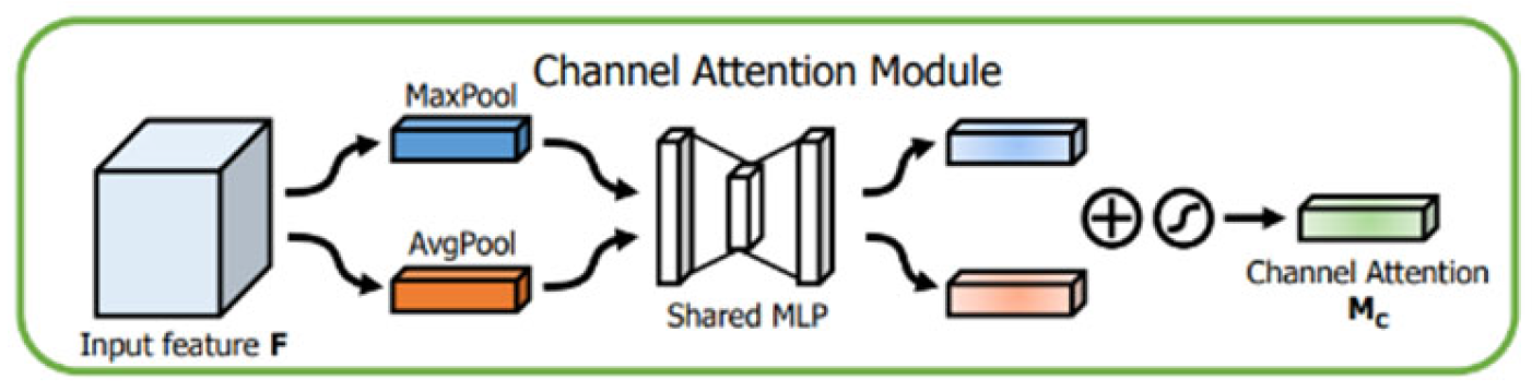
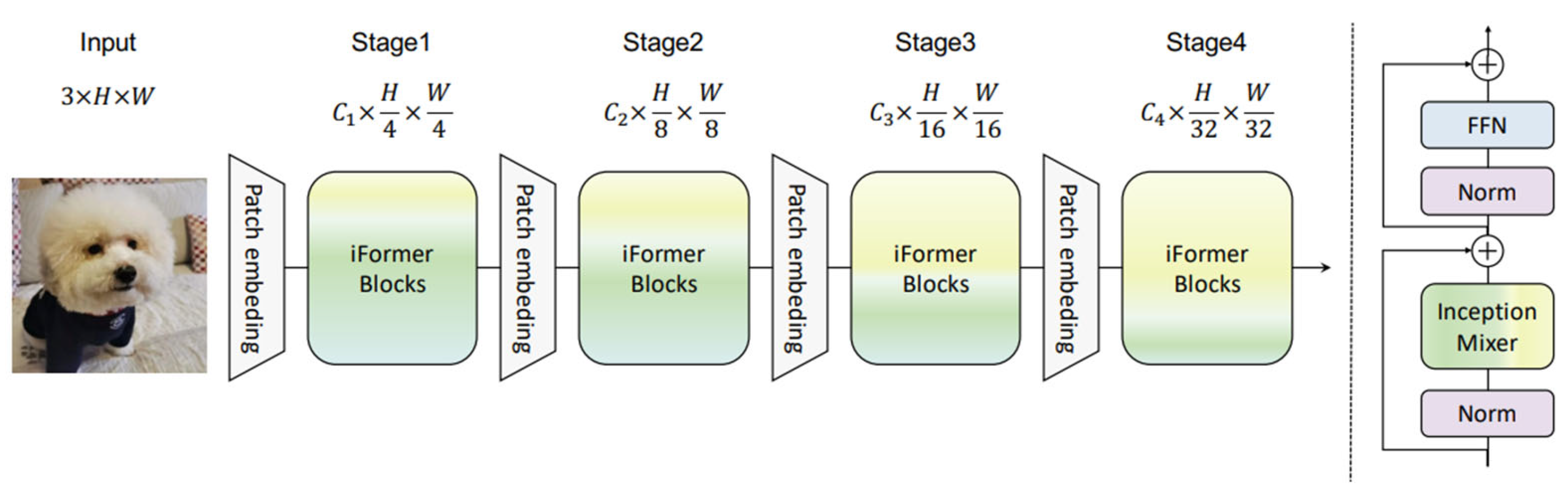
Figure 21.
LSTM architecture.

Figure 23.
Example of the Application of Optical Flow.

Figure 23.
Person 49 analysis - Facial variation (neutral state on the left, angry state on the right).
Figure 23.
Person 49 analysis - Facial variation (neutral state on the left, angry state on the right).

Figure 24.
Recording person 39 (from minute 1:30 to 1:59).

Figure 25.
Person 69 (from minute 0:55 to 1:20).

Figure 26.
Training loss graph for 3 classes.

Figure 27.
Training Accuracy Plot.

Figure 28.
ROC and AUC Plot for Three Classes.

Figure 29.
Training Accuracy Curve for Seven Classes.

Figure 30.
Confusion matrix for 7 classes during the testing stage.

Figure 31.
ROC and AUC curve for 7 classes.


Table 1.
Summary of the three datasets (CASME, SAMM, and SMIC).
| Feature | CASME II | SAMM | SMIC |
|---|---|---|---|
| Number of Sample | 255 | 159 | 164 |
| Participants | 35 | 32 | 16 |
| Ethnicities | Chinese | Chinese and 12 more | Chinese |
| Facial Resolution | 280x340 | 400x400 | 640x480 |
| Happiness (25) | Happinese (24) | ||
| Surprise (15) | Surprise (13) | Positive (51) | |
| Categories | Anger (99) | Anger (20) | Negative (70) |
| Sadness (20) | Sadness (3) | Surprise (43) | |
| Fear (1) Others (69) | Fear (7) Others (84) |
Table 2.
Performance comparison when applying Optical Flow across the three main datasets (CASME, SAMM, and SMIC).
Table 2.
Performance comparison when applying Optical Flow across the three main datasets (CASME, SAMM, and SMIC).
| Model version | Number of epochs | Training time | Loss of training | Accuracy | F1 score |
|---|---|---|---|---|---|
| Without Optical Flow | 60 | 1 hour 45 minutes and 58 seconds | 0.2108 | 90.28% | 0.8453 |
| With Optical Flow | 100 | 23 minutes and 55 seconds | 0.0986 | 90% | 0.8556 |
Table 3.
Training results for the three-class model.
| Training loss | Accuracy | Epochs | Training time | CPU usage | Memory usage |
|---|---|---|---|---|---|
| 0.1917 | 0.9474 | 60 | 8 minutes 38 seconds | 13.3% | 72.1% |
Table 4.
Performance metrics for the three-class model – Testing stage.
| F1-Score | Precision | Accuracy | Recall | Mean square error (MSE) | Mean absolute error (MAE) | |
|---|---|---|---|---|---|---|
| 0.8574 | 0.8127 | 0.8519 | 0.8127 | 0.2278 | 0.2175 | 0.8243 |
Disclaimer/Publisher’s Note: The statements, opinions and data contained in all publications are solely those of the individual author(s) and contributor(s) and not of MDPI and/or the editor(s). MDPI and/or the editor(s) disclaim responsibility for any injury to people or property resulting from any ideas, methods, instructions or products referred to in the content. |
© 2025 by the authors. Licensee MDPI, Basel, Switzerland. This article is an open access article distributed under the terms and conditions of the Creative Commons Attribution (CC BY) license (http://creativecommons.org/licenses/by/4.0/).
Copyright: This open access article is published under a Creative Commons CC BY 4.0 license, which permit the free download, distribution, and reuse, provided that the author and preprint are cited in any reuse.


