
Submitted:
29 October 2025
Posted:
30 October 2025
You are already at the latest version
Abstract
Adaptive cluster sampling (ACS) is a sampling method commonly employed when the population is rare and exhibits clustering. However, the initial sample selection may include units that do not satisfy the specified condition. To address this, general inverse sampling is incorporated into ACS, where the initial units are selected sequentially and termination criteria are applied to regulate the number of rare elements drawn from the population. The objective of this study is to develop an estimator of the population mean by utilizing auxiliary information within the framework of general inverse adaptive cluster sampling. The proposed estimator, constructed on the basis of a regression-type estimator, is analytically examined. A simulation study was conducted to validate the theoretical results. In this study, the region of interest was divided into 400 square units (20 rows by 20 columns). The results demonstrate that the proposed estimator, which incorporates auxiliary variables, consistently yields a lower variance than the conventional mean estimator without auxiliary information. This superiority holds across all scenarios considered, specifically when the predetermined number of rare units r ranges from two to ten. Therefore, the proposed estimator is shown to be more efficient than the estimator that does not employ auxiliary information.
Keywords:
adaptive cluster sampling
; general inverse sampling
; regression estimator
; auxiliary information
1. Introduction
Adaptive cluster sampling (ACS) has been recognized as an effective approach for studying population that is both rare and spatially clustered, with its introduction attributed to Thompson [1]. Initially, a set of initial sample units is drawn by employing simple random sampling without replacement (SRSWOR). Whenever one of these units meets the predefined criterion C for the variable of interest, the neighboring units of that sample are included. The procedure is then extended iteratively, such that any further units fulfilling the condition will result in the inclusion of their neighborhoods as well. This procedure is repeated until no further units satisfy the specified condition. In addition, if the initial unit does not satisfy condition C for the variable of interest, no augmentation occurs and the cluster size is one. The set of initial sample units selected and all neighborhood units that satisfy the condition is referred to as a network. ACS has been extensively applied in situations where populations are rare and exhibit clustered distributions. Its applications include forest ecosystem monitoring [2], herpetofauna surveys in tropical rainforests [3], assessments of sea lamprey larval distributions [4], and investigating freshwater mussel populations [5]. The method has also been used in hydroacoustic investigations [6] and research related to the COVID-19 pandemic [7,8,9]. Beyond ecological and epidemiological contexts, ACS has been further adapted to emerging domains, such as autonomous technologies and IoT-driven applications [10,11].
In many studies, the efficiency of estimation under ACS has been improved through the incorporation of auxiliary variables correlated with the variable of interest. A ratio-type estimator was introduced in [12], and subsequent modifications were proposed in [13]. An extension incorporating two auxiliary variables was presented in [14]. Further developments included ratio estimators based on known population parameters of the auxiliary variable, such as the coefficient of variation, kurtosis, and skewness [15,16]. Generalized exponential-type estimators were proposed in [17,18], while a generalized class of ratio-type estimators was developed in [19].
However, in ACS, the initial sample size is determined before sample selection, and it may happen that not all randomly selected units meet the specified condition C. Inverse ACS was proposed in [20], in which inverse sampling is applied within the ACS framework. In this design, the initial units are selected sequentially, and the sampling process is terminated according to stopping rules established to regulate the number of rare elements obtained from the population. However, in some cases of inverse sampling, the procedure may not be completed if the number of units meeting the specified condition is very small, while the stopping rules are set higher than the number of qualifying units. To address this limitation, general inverse sampling was introduced in [21], providing a more suitable approach for practical applications and subsequently applied to ACS. An estimator in general inverse ACS based on the Rao–Blackwell theorem was developed in [22], and the integration of unequal probability inverse sampling with ACS was investigated in [23].
As mentioned above, general inverse ACS has thus far been studied only in relation to the variable of interest. In certain cases, however, other variables correlated with the variable of interest may also be available, and their data can often be collected simultaneously without additional cost. Incorporating auxiliary variable information is a common strategy to enhance estimation precision. An estimator utilizing auxiliary variable information, specifically a regression-type estimator in general inverse sampling, was proposed in [24]. In this paper, an estimator was developed using auxiliary information in general ACS. Section 2 presents inverse sampling and general inverse sampling. Section 3 describes general inverse adaptive cluster sampling. Section 4 introduces the proposed estimator that uses auxiliary variable information in general inverse adaptive cluster sampling. Simulation studies are presented in Section 5, and finally, Section 6 presents the conclusions of the study.
2. Inverse Sampling and General Inverse Sampling
Population size units consist of the set of values . Let be the variable of interest and is the -value associated with the unit. The population is divided into two subgroups according to whether the -value satisfies the pre-condition C. Following the notation of [20], define the two subgroups by and , where is the unknown number of units of . In this sampling framework, the classification of a unit into subgroups is not determined in advance but becomes known only upon its selection. The sampling procedure involves sequentially selecting units at random from the target population. Sampling continues until a predetermined number of units from are sampled.
The estimator in inverse sampling was presented in [20]. Suppose a sample size is selected by SRSWOR. If at least units of are observed, then no further sampling is conducted. Otherwise, sampling continues sequentially until exactly units are selected. The total sequential sample size is defined as . Then an unbiased estimator of is:
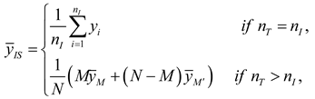 where ; is the index label of the members of .
; is the index label of the members of . In application, will be not known. The unbiased estimator of is .
The variance of is:
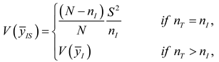
Using the variance of Murthy’s estimator [25],
, where is the probability of obtaining sample , is the conditional probability of obtaining given the unit was selected first, is the selection probability of unit in the first draw and .
For any sequential sampling design, the sampling procedure may not be able to complete in some situations. This may happen in an inverse sampling design because is too large or the population contains very few units satisfying condition C. General inverse sampling was proposed in [21]. Beginning with a sample size selected by SRSWOR, we stop further sampling if at least units from are selected. Otherwise, sampling continues until units from are obtained, but a limit is placed on the final sample size, such that . Then an unbiased estimator of is:
 where ,
and
.
The variance of is:
The unbiased estimator of the variance of is:
Here, ,
where is the probability of obtaining sample , given that units and were selected (in either order) on the first two draws. , and , .
3. General Inverse ACS
The integration of general inverse sampling with ACS is referred to as general inverse ACS. Under this design, if an initially selected unit satisfies the pre-specified condition C, the entire network to which that unit belongs is included in the sample. Consequently, the final sample comprises the initial units selected through general inverse sampling as well as all units that are members of the networks associated with those initial units. This also includes the edge units of these networks that sequentially satisfy condition C.
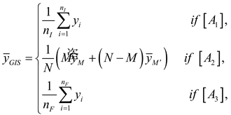
An estimator for the general inverse design with ACS [21]:
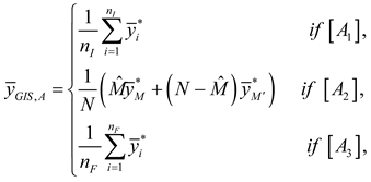 where is the average of the variable of interest in the network that includes unit of the initial sample, defined as , where denotes the network that includes unit , and is the number of units in that network.
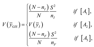
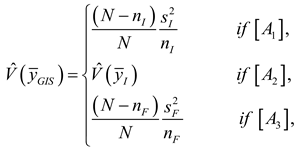
The variance of is:
and
.
The unbiased estimator of the variance of is:
 where , , and , .
4. Proposed Estimator in General Inverse ACS
Motivated by [24], the estimator can be calculated similar to by using the -variable. The modified regression estimator in general inverse ACS is , where is estimated by .
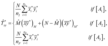 where and .
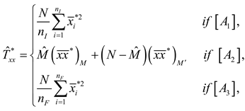 where and .
The bias of is
From , let , and let be estimated by . Therefore, .
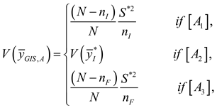
The variance of is:
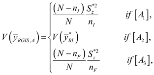
Using the variance of Murthy’s estimator,
and .
The estimator of the variance of is:
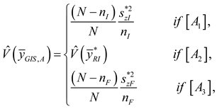 where , and
.
, ,
, ,
, and
, .
5. Simulation Studies and Discussion
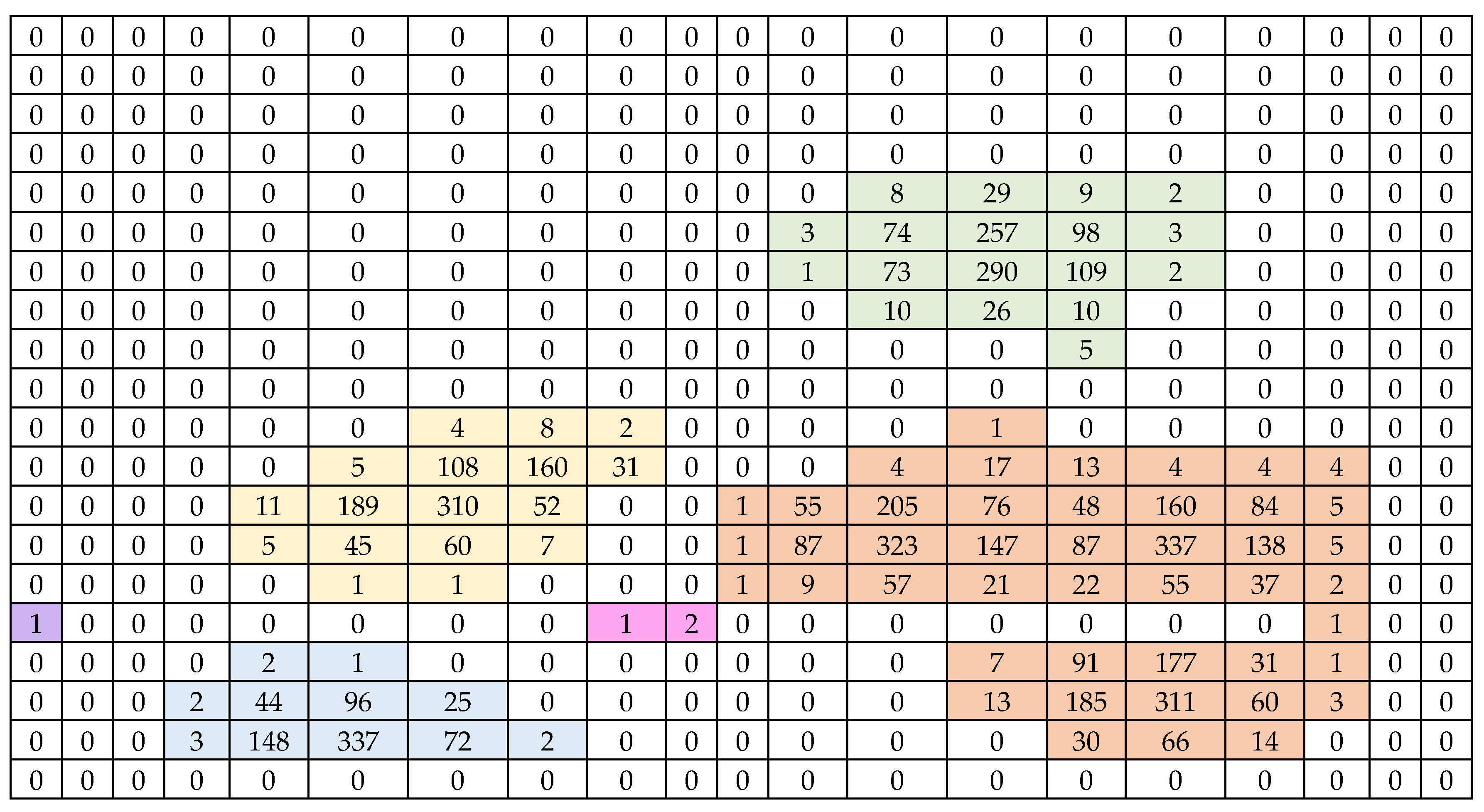
The population of the auxiliary variable and the variable of interest was generated using a Poisson cluster process [26]. The study area was subdivided into 400 square units (20 rows*20 columns). The population mean of -values is 59.7375, and the correlation coefficient between the -data and -data is 0.9973. The criterion for adding units to the sample were defined as .
Figure 1.
The population of the variable of interest ().
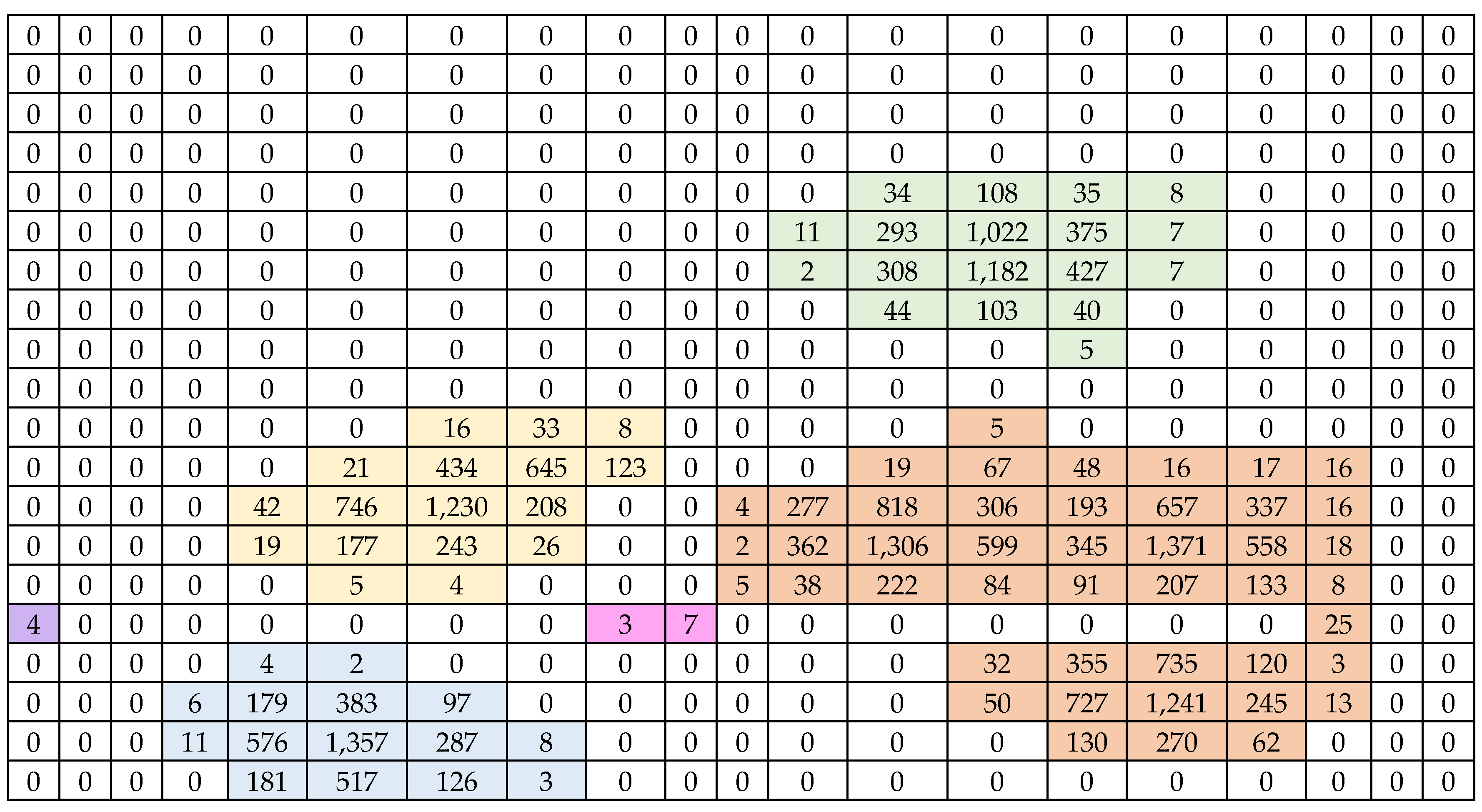
The shaded regions in different colors denote distinct networks.
Figure 2.
The population of the auxiliary variable ().
The position of the network is aligned with the data .
A total of 10,000 iterations were performed for each estimator. is the expected sequential sample size from general inverse sampling and is the expected final sample size, respectively.
The estimated variance of the estimators is defined as:
The relative efficiency of the proposed estimator, compared with , is defined as .
Since the proposed estimator is a biased estimator, the estimated absolute relative bias is defined as .
Discussion
Based on the data used in this study, the variable of interest and the auxiliary variable exhibit a linear relationship in the same direction. The results of the study are as follows:
From Table 1, since the proposed estimator is a biased estimator, the study found that as and increase, the estimated absolute relative bias of the proposed estimator decreases.
From Table 2, the study of the estimated variance of the estimators showed that as and increase, the estimated variance of the estimators decreases. When comparing the estimated variance between the proposed estimator that uses auxiliary variable and the estimator of the mean of the variable of interest without using auxiliary variable , it was found that has a lower estimated variance than in all cases. Moreover, the relative efficiency of the proposed estimator is greater than one in all cases, indicating that is more efficient than .
6. Conclusions
General inverse sampling was incorporated into ACS in [21], and this design is referred to as general inverse ACS. In this paper, an estimator of the mean of the variable of interest in general inverse ACS is developed using auxiliary variable, where the auxiliary variable has a linear relationship with the variable of interest. The study found that the proposed estimator is more efficient than the estimator of the mean of the variable of interest that does not use auxiliary variable, across all investigated scenarios.
In this study, the proposed estimator was motivated by the work in [24], which introduced a regression-type estimator utilizing information from a single auxiliary variable. Therefore, future research could focus on developing estimators that use information from other auxiliary variables, such as the coefficient of variation of the auxiliary variable or the correlation coefficient between the auxiliary variable and the variable of interest as well as the use of more than one auxiliary variable.
Author Contributions
Conceptualization, N.C. and P.G.; methodology, S.W. and N.C.; software, N.C.; validation, M.C. and C.B.; formal analysis, N.C. and M.C.; investigation, S.W. and P.G.; resources, N.C. and C.B.; data curation, N.C. and C.B.; writing—original draft preparation, N.C. and M.C.; writing—review and editing, P.G. and S.W.; visualization, P.G. and C.B.; supervision, N.C. and P.G.; project administration, N.C.; funding acquisition, N.C. All authors have read and agreed to the published version of the manuscript.
Funding
This research project was financially supported by Mahasarakham University.
Data Availability Statement
The original contributions presented in this study are included in the article. Further inquiries can be directed to the corresponding author.
Conflicts of Interest
The authors have no conflicts of interest to declare that are relevant to the content of this article.
References
- Thompson, S.K. Adaptive cluster sampling. J. Am. Statist. Assoc. 1990, 85, 1050–1059. [Google Scholar] [CrossRef]
- Magnussen, S.; Kurz, W.; Leckie, D.G.; Paradine, D. Adaptive cluster sampling for estimation of deforestation rates. Eur. J. For. Res. 2005, 124, 207–220. [Google Scholar] [CrossRef]
- Noon, B.R.; Ishwar, N.M.; Vasudevan, K. Efficiency of adaptive cluster and random sampling in detecting terrestrial herpetofauna in a tropical rainforest. Wildl. Soc. Bull. 2006, 34, 59–68. [Google Scholar] [CrossRef]
- Sullivan, W.P.; Morrison, B.J.; Beamish, F.W.H. Adaptive cluster sampling: Estimating density of spatially autocorrelated larvae of the sea lamprey with improved precision. J. Great Lakes Res. 2008, 34, 86–97. [Google Scholar] [CrossRef]
- Smith, D.R.; Villella, R.F.; Lemarié, D.P. Application of adaptive cluster sampling to low-density populations of freshwater mussels. Environ. Ecol. Stat. 2003, 10, 7–15. [Google Scholar] [CrossRef]
- Conners, M.E.; Schwager, S.J. The use of adaptive cluster sampling for hydroacoustic surveys. ICES J. Mar. Sci. 2002, 59, 1314–1325. [Google Scholar] [CrossRef]
- Olayiwola, O.M.; Ajayi, A.O.; Onifade, O.C.; Wale-Orojo, O.; Ajibade, B. Adaptive cluster sampling with model based approach for estimating total number of Hidden COVID-19 carriers in Nigeria. Stat. J. IAOS 2020, 36, 103–109. [Google Scholar] [CrossRef]
- Chandra, G.; Tiwari, N.; Nautiyal, R. Adaptive cluster sampling-based design for estimating COVID-19 cases with random samples. Curr. Sci. 2021, 120, 1204–1210. [Google Scholar] [CrossRef]
- Stehlík, M.; Kiseľák, J.; Dinamarca, A.; Alvarado, E.; Plaza, F.; Medina, F.A.; Stehlíková, S.; Marek, J.; Venegas, B.; Gajdoš, A.; et al. REDACS: Regional emergency-driven adaptive cluster sampling for effective COVID-19 management. Stoch. Anal. Appl. 2022, 41, 474–508. [Google Scholar] [CrossRef] [PubMed]
- Hwang, J.; Bose, N.; Fan, S. AUV adaptive sampling methods: A Review. Appl. Sci. 2019, 9, 3145. [Google Scholar] [CrossRef]
- Giouroukis, D.; Dadiani, A.; Traub, J.; Zeuch, S.; Markl, V. A survey of adaptive sampling and filtering algorithms for the internet of things. In Proceedings of the 14th ACM International Conference on Distributed and Event- Based Systems, Montreal, QC, Canada, 13–17 July 2020; pp. 27–38. [Google Scholar] [CrossRef]
- Chao, C.T. Ratio estimation on adaptive cluster sampling. J. Chin. Stat. Assoc. 2004, 42, 307–327. [Google Scholar] [CrossRef]
- Dryver, A.L.; Chao, C.T. Ratio estimators in adaptive cluster sampling. Environmetric 2007, 18, 607–620. [Google Scholar] [CrossRef]
- Chutiman, N.; Kumphon, B. Ratio estimator using two auxiliary variables for adaptive cluster sampling. Thail. Stat. 2008, 6, 241–256. [Google Scholar]
- Chutiman, N. Adaptive cluster sampling using auxiliary variable. J. Math. Stat. 2013, 9, 249–255. [Google Scholar] [CrossRef]
- Yadav, S.K.; Misra, S.; Mishra, S. Efficient estimator for population variance using auxiliary variable. Am. J. Oper. Res. 2016, 6, 9–15. [Google Scholar] [CrossRef]
- Chaudhry, M.S.; Hanif, M. Generalized exponential-cum-exponential estimator in adaptive cluster sampling. Pak. J. Stat. Oper. Res. 2015, 11, 553–574. [Google Scholar] [CrossRef]
- Chaudhry, M.S.; Hanif, M. Generalized difference-cum-exponential estimator in adaptive cluster sampling. Pak. J. Stat. 2017, 33, 335–367. [Google Scholar]
- Bhat, A.A.; Sharma, M.; Shah, M.; Bhat, M. Generalized ratio type estimator under adaptive cluster sampling. J. Sci. Res. 2023, 67, 46–51. [Google Scholar] [CrossRef]
- Christman, M.C.; Lan, F. Inverse Adaptive Cluster Sampling. Biometrics, 2001, 57, 1096–1105. [Google Scholar] [CrossRef]
- Salehi, M.; Seber, G.A.F. A general inverse sampling scheme and its application to adaptive cluster sampling. Aust. N. Z. J. Stat. 2004, 46, 483–494. [Google Scholar] [CrossRef]
- Pochai, N. An Improved the Estimator in Inverse Adaptive Cluster Sampling. Thail. Stat. 2008, 6, 15–26, https://ph02.tci-thaijo.org/index.php/thaistat/article/view/34329. [Google Scholar]
- Sangngam, P. Unequal Probability Inverse Adaptive Cluster Sampling. Chiang Mai J. Sci. 2013, 40, 736–742. [Google Scholar]
- Moradi, M.; Salehi, M.; Brown, J.A.; Karimi, N. (2011). Regression estimator under inverse sampling to estimate arsenic contamination. Environmetrics. 2011, 22, 894–900. [Google Scholar] [CrossRef]
- Salehi, M.; Seber, G.A.F. (2001). Theory & Methods: A New Proof of Murthy's Estimator which Applies to Sequential Sampling. Aust. N. Z. J. Stat. 2001, 43, 281–286. [Google Scholar]
- Subzar, M.; Alqurashi, T.; Chandawat, D.; Tamboli, S.; Raja, T. A.; Attri, A.K.; Wani, S.A. Generalized robust regression techniques and adaptive cluster sampling for efficient estimation of population mean in case of rare and clustered populations. Sci Rep. 2025, 15, 2069. [Google Scholar] [CrossRef]

Table 1.
The estimated absolute relative bias of the proposed estimator for the population mean of the variable of interest.
Table 1.
The estimated absolute relative bias of the proposed estimator for the population mean of the variable of interest.
| 2 | 5 | 8.7335 | 57.0359 | 0.37475 |
| 2 | 10 | 11.2945 | 65.1829 | 0.19846 |
| 2 | 15 | 15.4288 | 75.4269 | 0.06664 |
| 3 | 5 | 12.2907 | 69.8711 | 0.21408 |
| 3 | 10 | 13.4347 | 72.8004 | 0.20585 |
| 3 | 15 | 16.5289 | 79.6913 | 0.16196 |
| 3 | 20 | 20.4772 | 87.5785 | 0.04360 |
| 4 | 10 | 16.6089 | 82.3383 | 0.14986 |
| 4 | 15 | 18.0372 | 84.5381 | 0.15376 |
| 4 | 20 | 21.3896 | 91.4283 | 0.12636 |
| 5 | 15 | 21.3911 | 91.4934 | 0.13535 |
| 5 | 20 | 23.6009 | 95.6987 | 0.13861 |
| 5 | 25 | 26.2153 | 100.5247 | 0.09379 |
| 5 | 30 | 30.5074 | 106.9697 | 0.04137 |
| 10 | 30 | 41.5436 | 122.0440 | 0.09839 |
| 10 | 40 | 44.2324 | 124.5140 | 0.08867 |
| 10 | 50 | 44.2324 | 130.6097 | 0.05299 |
Table 2.
The estimated variance of the estimators for the population mean of the variable of interest and the relative efficiency of the proposed estimator compared with .
Table 2.
The estimated variance of the estimators for the population mean of the variable of interest and the relative efficiency of the proposed estimator compared with .
| 2 | 5 | 8.7335 | 57.0359 | 2,242.0274 | 1,359.3310 | 1.6494 |
| 2 | 10 | 11.2945 | 65.1829 | 1,174.3768 | 663.9508 | 1.7688 |
| 2 | 15 | 15.4288 | 75.4269 | 730.6367 | 579.0399 | 1.2618 |
| 3 | 5 | 12.2907 | 69.8711 | 1,772.1519 | 1,287.5967 | 1.3763 |
| 3 | 10 | 13.4347 | 72.8004 | 863.4391 | 389.3139 | 2.2178 |
| 3 | 15 | 16.5289 | 79.6913 | 795.5099 | 426.5605 | 1.8649 |
| 3 | 20 | 20.4772 | 87.5785 | 526.7130 | 406.0654 | 1.2971 |
| 4 | 10 | 16.6089 | 82.3383 | 742.8746 | 422.3135 | 1.7591 |
| 4 | 15 | 18.0372 | 84.5381 | 544.0685 | 232.7903 | 2.3372 |
| 4 | 20 | 21.3896 | 91.4283 | 536.4767 | 285.0840 | 1.8818 |
| 5 | 15 | 21.3911 | 91.4934 | 516.0823 | 241.1235 | 2.1403 |
| 5 | 20 | 23.6009 | 95.6987 | 524.0002 | 228.0293 | 2.2980 |
| 5 | 25 | 26.2153 | 100.5247 | 398.3312 | 219.3141 | 1.8163 |
| 5 | 30 | 30.5074 | 106.9697 | 344.7272 | 228.7729 | 1.5069 |
| 10 | 30 | 41.5436 | 122.0440 | 339.7744 | 167.0369 | 2.0341 |
| 10 | 40 | 44.2324 | 124.5140 | 194.7799 | 72.3611 | 2.6918 |
| 10 | 50 | 44.2324 | 130.6097 | 152.7576 | 93.7495 | 1.6294 |
Disclaimer/Publisher’s Note: The statements, opinions and data contained in all publications are solely those of the individual author(s) and contributor(s) and not of MDPI and/or the editor(s). MDPI and/or the editor(s) disclaim responsibility for any injury to people or property resulting from any ideas, methods, instructions or products referred to in the content. |
© 2025 by the authors. Licensee MDPI, Basel, Switzerland. This article is an open access article distributed under the terms and conditions of the Creative Commons Attribution (CC BY) license (https://creativecommons.org/licenses/by/4.0/).
Copyright: This open access article is published under a Creative Commons CC BY 4.0 license, which permit the free download, distribution, and reuse, provided that the author and preprint are cited in any reuse.


