Optimal Control in Financial Markets for the Uncertain Volatility Model

1. Introduction

The first model to describe the evolution of stock prices was the Bachelier linear model [1]. One of the fundamental shortcomings of the Bachelier model is the fact that stock prices can take negative values. In [2], Samuelson proposed to describe stock prices by geometric Brownian motion. In other words, Samuelson proposed to consider that the logarithms of stock prices obey a Bachelier-type linear model. In [3], Black and Scholes proposed a standard diffusion model of the (B,S)-market and obtained a formula for the fair value of European-type call options. A significant shortcoming of this model is the fact that the coefficients of drift, interest rate and volatility are constant, although in reality they change over time. In this regard, the so-called smile-effect should be noted, which is a fact that is not explained by the standard diffusion model, which has led to its various generalizations and improvements. The essence of the smile-effect is as follows. The Black and Scholes formula provides an explicit relationship between the fair price and volatility, the expiration date, and the contract price. We can look at actual option prices in financial markets and compare them with theoretical values. We can then use this equation to calculate the implied volatility, which depends on the expiration date and the contract price. It has been experimentally established that:

• For a fixed contract price, implied volatility changes with the expiration date.
• For a fixed expiration date, implied volatility changes with the contract price, being a downward-convex function, which explains the name “smile-effect”.

To account for the first observed effect, Merton proposed considering drift and volatility as functions of time in the standard model [4], and such schemes are indeed used in financial markets, especially in the settlement of American-style options.

To take into account the second observed effect, a wide variety of complications of the standard model are introduced. In [5], models of the “diffusion with jumps” type are presented. In [6], models with stochastic interest rates are presented. In [7,8], the Dupiri model is proposed, in which the drift is a function of time, and volatility depends on the time and the cost of the risky asset. In the mentioned works, Dupiri also showed that the ideas of arbitrage-free market conditions and market completeness make it possible to estimate the unknown volatility using knowledge of the actually observed prices of standard European-type call options with fixed exercise time and exercise price. In [9,10,11,12,13], models of stochastic volatility are presented. In [14], the Heston stochastic volatility model is proposed. In [15,16,17,18,19,20,21], various numerical methods for calculating option prices in the Heston model are proposed. In [15], a tree method is proposed for calculating the prices of American options in the Heston model. In [16], a hybrid method for estimating option prices in the Heston model is proposed. In [17], a Monte Carlo method for calculating the prices of American options in the Heston model is proposed. In [18], a numerical method for calculating the prices of barrier options in the Heston model is constructed. In [19], finite-difference methods for calculating option prices in the Heston model are presented, as well as algorithms for estimating the model parameters. In [20], an algorithm for calculating option prices in the Heston model using artificial neural networks is presented. In [21], a numerical implementation of European-type option prices in the Heston model using integral transformations is proposed. In [22,23,24,25,26], models with disorder are proposed. Cases of observed [22,23] and unobserved [24,25,26] disorder are considered. In [27,28,29], models of uncertain volatility are considered. In particular, [27] examines two models of uncertain volatility and presents formulas for calculating the fair value range of a European-style option.

This article considers a model of uncertain volatility, a generalization of the well-known Black-Scholes model. For the uncertain volatility model, the upper and lower prices of the payment obligation are represented as a submartingale and supermartingale, respectively. The Hamilton-Jacobi-Bellman equations are derived for calculating these. The resulting equations are transformed into nonlinear heat equations with a boundary condition. Theorems have been proven that if the boundary condition is a continuous and convex function, then the solutions of nonlinear heat equations are convex functions that satisfy the linear heat equations.

2. Black-Scholes Model

Let $W\left(t\right)$ be a standard Wiener process on a stochastic basis $\langle C[0,T],{\left(F_t^W\right)}_{t\ge 0},F_T^W,P^W\rangle$. Consider the equation for the discounted stock price process $dS\left(t\right)=S\left(t\right)\sigma dW\left(t\right)$ with initial condition $S\left(0\right)=S_0$. A process $Y\left(t\right)=E(f\left(S\left(T\right)\right)\mid F_t^W)$, where the function $f\left(x\right)\ge 0$ and the mathematical expectation $E\left(f\right(S\left(T\right)\left)\right)$ is finite, is the portfolio capital. Capital can be represented as a function of time and asset value $Y\left(t\right)=V(t,S(t\left)\right),$ where the function $V(t,x)\in C^{1,2}$ has the form $V(t,x)=E_{t,x}\left(f\left(S\left(T\right)\right)\right).$ This mathematical expectation $E_{t,x}\left(f\left(S\left(T\right)\right)\right)$ is calculated under the condition that the value of the Markov random process $S\left(t\right)$ at time t is equal to x. This function is a solution to the Cauchy problem [30]:

$${\displaystyle \frac{\partial V}{\partial t}}+{\displaystyle \frac{{\sigma }^2}{2}}{\displaystyle \frac{{\partial }^{2}V}{\partial x^2}}=0,V(T,x)=f\left(x\right).$$

(1)

The solution to this equation is known [30]:

$$V(t,x)={\displaystyle \frac{1}{\sqrt{2\pi }}}{\int }_{-\infty }^{+\infty }f\left(xexp\left(-{\displaystyle \frac{{\sigma }^2}{2}}(T-t)+\sigma \sqrt{T-t}y\right)\right)exp\left(-{\displaystyle \frac{y^2}{2}}\right)dy.$$

For example, in financial mathematics, the problem of calculating the fair price of a European call option with a contract price K and an interest rate r on a risk-free asset is relevant. For this problem the function $f\left(x\right)=exp(-rT){(x-K)}^{+}$, where ${\left(x\right)}^{+}=max(x,0)$. Function $V(t,x)=x\mathsf{\Phi }\left(d_1(t,x)\right)-K{e}^{-r(T-t)}\mathsf{\Phi }\left(d_2(t,x)\right)$, process $Y\left(t\right)$ and fair price for a European call option $C=Y\left(0\right)=V(0,S_0)$. As a result, the fair price is calculated using the formula $C=S_0\mathsf{\Phi }\left(d_1(0,S_0)\right)-K{e}^{-rT}\mathsf{\Phi }\left(d_2(0,S_0)\right),$ where $\mathsf{\Phi }\left(x\right)$ denotes the standard normal distribution function, $d_1(t,x)={\displaystyle \frac{ln(x/K)+(r+{\sigma }^2/2)(T-t)}{\sigma \sqrt{T-t}}},$$d_2(t,x)=d_1(t,x)-\sigma \sqrt{T-t}.$

3. Heston’s Model

Heston’s model considers a two-dimensional Wiener process $W\left(t\right)=\left(\begin{array}{c}{W}_1\left(t\right)\\ W_2\left(t\right)\end{array}\right)$ with $dW\left(t\right)\in N\left(\begin{array}{cc}0,& \left(\begin{array}{cc}1& \rho \\ \rho & 1\end{array}\right)dt\end{array}\right).$ The equation for the discounted stock price process is $dS\left(t\right)=S\left(t\right)\sqrt{\sigma \left(t\right)}d{W}_1\left(t\right),$$S\left(0\right)=S_0,$ where $d\sigma \left(t\right)=k(\theta -\sigma \left(t\right))dt+\nu \sqrt{\sigma \left(t\right)}d{W}_2\left(t\right),\sigma \left(0\right)={\sigma }_0.$ The quantities $k,\theta ,\nu >0$ are the model parameters. If $2k\theta \ge {\nu }^2$ and ${\sigma }_0>0$, then the process $\sigma \left(t\right)$ is strictly positive, which is important since volatility is non-negative.

The following interpretation can be given to the parameters of the stochastic dispersion process. Denoting $F\left(t\right)=E\sigma \left(t\right)$, we obtain the equation $F\left(t\right)={\sigma }_0+k{\int }_0^t(\theta -F\left(s\right))ds,$ the solution of which is $F\left(t\right)=\theta +({\sigma }_0-\theta )e^{-kt}.$ Thus, the process $\sigma \left(t\right)$ has the property of returning to a level $\theta$, called the long-run average. The parameter k specifies the speed of return to $\theta$. The parameter $\nu$ is called the “volatility of volatility” and it controls how strong the volatility swings are.

Let’s consider $F^2\left(t\right)=E{\sigma }^2\left(t\right)$. The application of the Ito formula allows us to write an equation $d{F}^2=(-2k{F}^2+\phi )dt,$ the solution of which

$$F^2\left(t\right)={\displaystyle \frac{1}{2k}}\left(F\left(t\right)\left(2k\right)\theta +{\nu }^2-(2k{F}^2\left(0\right)+(F\left(0\right)\left(2k\right)\theta +{\nu }^2)exp(-2kt)\right)$$

allows us to find the volatility dispersion $D\sigma \left(t\right)=F^2\left(t\right)-{\left(F\left(t\right)\right)}^2$, which at $k\to \infty$ tends to zero and “reduces” the Heston model to the Black-Scholes model.

For the Heston model, we consider the process $Y\left(t\right)=E(f\left(S\left(T\right)\right)\mid F_t^W)$, where the function $f\left(x\right)\ge 0$ and the mathematical expectation $E\left(f\right(S\left(T\right)\left)\right)$ is finite, which can be represented by the equality: $Y\left(t\right)=V(t,S(t),\sigma (t\left)\right)$. Note that we need a function of three variables. The function $V(t,x,y)\in C^{1,2,2}$ is the conditional mathematical expectation: $V(t,x,y)=E_{t,x,y}\left(f\left(S\left(T\right)\right)\right)$, is the solution to the Cauchy problem [14]:

$${\displaystyle \frac{\partial V}{\partial t}}+{\displaystyle \frac{\partial V}{\partial y}}k(\theta -y)+{\displaystyle \frac{1}{2}}{\displaystyle \frac{{\partial }^{2}V}{\partial x^2}}{x}^{2}y+{\displaystyle \frac{1}{2}}{\displaystyle \frac{{\partial }^{2}V}{\partial y^2}}{\nu }^{2}y+{\displaystyle \frac{{\partial }^{2}V}{\partial x\partial y}}x\nu y\rho =0,V(T,x,y)=f\left(x\right).$$

(2)

To obtain an approximate solution to Equation (2), we apply the method of lines [31], for which we divide time into segments of equal length, equal to $h={\displaystyle \frac{T}{N}}$. In accordance with this division, we represent Equation (2) as a system of elliptic partial differential equations with respect to spatial variables (the method of lines with respect to time) $V(i-1,x,y)=$

$$=h\left(V_y(i,x,y)k(\theta -y)+{\displaystyle \frac{1}{2}}{V}_{xx}(i,x,y)x^{2}y+{\displaystyle \frac{1}{2}}{V}_{yy}(i,x,y){\nu }^{2}y+V_{xy}(i,x,y)x\nu y\rho \right)+V(i,x,y),$$

$V(N,x,y)=f\left(x\right).$ The notation $V(i,x,y)=V(ih,x,y)$ is used. Besides the method of lines, other computational methods for computing the function V can be considered, one of them was proposed directly by Heston [14] for the already considered problem of calculating the fair price of a European call option.

Let’s consider a call option for the Heston model similar to how we did for the Black-Scholes model. Let us state a theorem.

Theorem 1.

[14] The price at time t of a call option with contract price K and exercise time T is equal:

$$\begin{array}{cc}\hfill V(t,x,y)& =exp(-r(T-t\left)\right)F(t,lnx,y)\hfill \\ \hfill F(t,x,y)& =e^x\tilde{\Pi }(t,x,y)-K\Pi (t,x,y)\hfill \\ \hfill \Pi (t,x,y)& ={\displaystyle \frac{1}{2}}+{\displaystyle \frac{1}{\pi }}{\int }_0^{\infty }Re\left({\displaystyle \frac{e^{-iulnK}\varphi (t,x,y,u)}{iu}}\right)du\hfill \\ \hfill \tilde{\Pi }(t,x,y)& ={\displaystyle \frac{1}{2}}+{\displaystyle \frac{1}{\pi }}{\int }_0^{\infty }Re\left({\displaystyle \frac{e^{-iulnK}\tilde{\varphi }(t,x,y,u)}{iu}}\right)du\hfill \\ \hfill \varphi (t,x,y,u)& =exp\left(C\right(T-t,u)+D(T-t,u)y+iux)\hfill \\ \hfill \tilde{\varphi }(t,x,y,u)& ={\displaystyle \frac{\varphi (t,x,y,u-i)}{\varphi (t,x,y,-i)}}\hfill \\ \hfill C(\tau ,u)& =riu\tau +{\displaystyle \frac{k\theta }{{\nu }^2}}\left((k-\rho \nu iu-d\left(u\right))\tau -2ln\left({\displaystyle \frac{1-g\left(u\right)e^{-d\left(u\right)\tau }}{1-g\left(u\right)}}\right)\right)\hfill \\ \hfill D(\tau ,u)& ={\displaystyle \frac{k-\rho \nu iu-d\left(u\right)}{{\nu }^2}}\left({\displaystyle \frac{1-e^{-d\left(u\right)\tau }}{1-g\left(u\right)e^{-d\left(u\right)\tau }}}\right)\hfill \\ \hfill d\left(u\right)& =\sqrt{{(\rho \nu iu-k)}^2+{\nu }^2(iu+u^2)}\hfill \\ \hfill g\left(u\right)& ={\displaystyle \frac{\rho \nu iu-k+d\left(u\right)}{\rho \nu iu-k-d\left(u\right)}}\hfill \end{array}$$

(3)

Let’s split the interval $[0,T]$ into N parts with a step $h={\displaystyle \frac{T}{N}}$ and consider the discrete Heston model:

$$\left\{\begin{array}{c}\Delta S_n=S_{n-1}\sqrt{{\sigma }_{n}h}{\delta }_n^1\hfill \\ \Delta {\sigma }_n=k(\theta -{\sigma }_{n-1})h+\nu \sqrt{{\sigma }_{n-1}h}{\delta }_n^2\hfill \end{array}\right.$$

(4)

$n=1,\dots ,N$.

Let us consider two implementations of model (4).

• Sequences ${\left({\delta }_n^1\right)}_{n=1}^N$ and ${\left({\delta }_n^2\right)}_{n=1}^N$ consist of independent Rademacher random variables with $\mathrm{cov}({\delta }_n^1,{\delta }_n^2)=\rho$.
• The sequence $\left(\begin{array}{c}{\delta }_n^1\\ {\delta }_n^2\end{array}\right)$ consists of independent random vectors distributed according to a two-dimensional normal law with zero mathematical expectation and a covariance matrix $\left(\begin{array}{cc}1& \rho \\ \rho & 1\end{array}\right).$

As before, we are now interested in a discrete process $Y_n=E(f\left(S_N\right)\mid F_n)$, where the function $f\left(x\right)\ge 0$ and the mathematical expectation $E\left(f\left(S_N\right)\right)$ is finite. The process $Y_n$ can be represented as $Y_n=V(n,S_n,{\sigma }_n)$, where the function V is the conditional mathematical expectation $V(n,x,y)=E(f\left(S_N\right)\mid S_n=x,{\sigma }_n=y)$. The discrete model allows calculating conditional mathematical expectations using the Monte Carlo method. For any discrete time n it is necessary to reproduce the required number of trajectory residuals; for each trajectory residual, it is necessary to generate random variables ${\delta }_i^1,{\delta }_i^2$. Computationally, the first option is preferable to the second.

The fair price can be calculated using recurrence formulas that use a sequence of Bellman functions $V(i,x,y)$, related by the Bellman equation $V(i-1,x,y)=EV(i,x+\Delta S_i,y+\Delta {\sigma }_i)$. We apply the second-order Taylor formula and discard terms of order of smallness $h^2$, as a result we obtain:

$$\begin{array}{cc}\hfill V(i-1,x,y)& =EV(i,x+\Delta S_i,y+\Delta {\sigma }_i)=\hfill \\ \hfill & =V(i,x,y)+V_x(i,x,y)E\Delta S_i+V_y(i,x,y)E\Delta {\sigma }_i+{\displaystyle \frac{1}{2}}{V}_{xx}(i,x,y)E{\left(\Delta S_i\right)}^2+\hfill \\ \hfill & V_{xy}(i,x,y)E\Delta S_{i}E\Delta {\sigma }_i+{\displaystyle \frac{1}{2}}{V}_{yy}(i,x,y)E{\left(\Delta {\sigma }_i\right)}^2=\hfill \\ \hfill & =h\left(V_y(i,x,y)k(\theta -y)+{\displaystyle \frac{1}{2}}{V}_{xx}(i,x,y)x^{2}y+{\displaystyle \frac{1}{2}}{V}_{yy}(i,x,y){\nu }^{2}y+V_{xy}(i,x,y)x\nu \rho \right),\hfill \\ \hfill & V(N,x,y)=f\left(x\right).\hfill \end{array}$$

This system of equations is completely identical to the system of equations for the line method, and is the same for both the first and second variants.

This fact allows us to assert that the discrete Heston model, both the first and second variants, are equally good approximations of the continuous Heston model. Specifically, the approximation error when calculating the function $V(t,x,y)$ in the discrete model and in the line method are the same and are of the order of h provided that the system of differential equations is solved with the required accuracy and the number of iterations in the Monte Carlo method is of the order of ${\displaystyle \frac{1}{h^2}}$. It should be noted that the Monte Carlo method in its binary implementation has undeniable advantages over other computational methods, since at each iteration it requires simple calculations and the generation of two random variables uniformly distributed over the interval $[0,1]$.

4. Uncertain Volatility Model

Let us consider the Banach space of bounded functions $l_{\infty }\left([0,T]\right)$, probability space $\langle l_{\infty },B\left(l_{\infty }\right),P\rangle$. The set ${\Sigma }_t=\{x\in R^{+}:\exists (\sigma \in \Sigma )\wedge (\sigma \left(t\right)=x)\},\Sigma \in l_{\infty }$ is compact for every $t\in [0,T]$. Based on any probability measure $P\in \mathcal{P}$ one can define a measure $P_{\Sigma }\left(A\right)=\left\{\begin{array}{cc}P(A·\Sigma )/P\left(\Sigma \right),\hfill & \mathrm{if}P\left(\Sigma \right)\ne 0\hfill \\ 0,\hfill & \mathrm{if}P\left(\Sigma \right)=0\hfill \end{array}\right.$ Let us denote the family of such measures by ${\mathcal{P}}_{\Sigma }$.

Let us consider independent random processes, each defined on its own stochastic basis $\langle C[0,T],{\left(F_t^W\right)}_{t\ge 0},F_T^W,P^W\rangle$ and $\langle l_{\infty }\left([0,T]\right),{\left(F_t^X\right)}_{t\ge 0},F_T^X,P_{\Sigma }\rangle .$ Let’s consider the equation for the discounted stock price process $dS\left(t\right)=S\left(t\right)X\left(t\right)dW\left(t\right)$ with initial conditions $S\left(0\right)=S_0,X\left(0\right)=X_0.$ This process is a martingale with respect to filtration ${(F_t^W\times F_t^X)}_{t\ge 0}$ and any measure from $P^W\times {\mathcal{P}}_{\Sigma }$, since the Novikov condition is satisfied [6].

The problem is to calculate the submartingale $Y\left(t\right)={sup}_{Q\in P^W\times {\mathcal{P}}_{\Sigma }}{E}_{Q}f(S_T\mid F_t^W)$. Let $m\left(t\right)$ be the lower envelope, and $M\left(t\right)$ the upper envelope of the family of slices ${\Sigma }_t$. Let’s consider the probability space $\langle \left[m\right(t),M(t\left)\right],B\left(\right[m\left(t\right),M\left(t\right)\left]\right),\mathcal{P}\left(t\right)\rangle$. To calculate the submartingale $Y\left(t\right)$ we use the Hamilton-Jacobi-Bellman equation ${\displaystyle \frac{\partial V}{\partial t}}+{\displaystyle \frac{x^2}{2}}{sup}_{P\in \mathcal{P}\left(t\right)}E{\displaystyle \frac{{\partial }^2\overline{V}}{\partial x^2}}=0,$ which is transformed into a nonlinear heat equation

$${\displaystyle \frac{\partial \overline{V}}{\partial t}}+{\displaystyle \frac{x^2}{2}}\left[{\displaystyle \frac{M^2\left(t\right)-m^2\left(t\right)}{2}}\left|{\displaystyle \frac{{\partial }^2\overline{V}}{\partial x^2}}\right|+{\displaystyle \frac{M^2\left(t\right)+m^2\left(t\right)}{2}}{\displaystyle \frac{{\partial }^2\overline{V}}{\partial x^2}}\right]=0$$

(5)

with a boundary condition $\overline{V}(T,x)=f\left(x\right)$.

Theorem 2.

[32] If $f\left(x\right)$ is a continuous function, then there exists a unique viscosity solution of Equation (5) $Y\left(t\right)=\overline{V}(t,x)$, which is a submartingale.

Theorem 3.

If $f\left(x\right)$ is a continuous and convex function, then the solution to the nonlinear heat Equation (5) is a convex function satisfying the linear heat equation:

$${\displaystyle \frac{\partial \overline{V}}{\partial t}}+{\displaystyle \frac{x^2{M}^2\left(t\right)}{2}}{\displaystyle \frac{{\partial }^2\overline{V}}{\partial x^2}}=0.$$

(6)

Proof 

(Proof). Let us consider a discrete model that arises as a result of dividing an interval $[0,T]$ into N equal parts $S_n^N=S_{n-1}^N\left(1+\sqrt{{\displaystyle \frac{T}{N}}}{X}_{n-1}^N{\epsilon }_n\right),$ where ${\epsilon }_n$ are independent Rademacher random variables, $S^N$ is a discrete version of the process S, and $X^N$ is a discrete version of the process X. For this model, we consider a sequence of functions $V_n^N\left(x\right)={max}_{\begin{array}{c}{m}_n^N\le x_n^N\le M_n^N,...,m_N^N\le x_N^N\le M_N^N\end{array}}E\left(f\left(S_N^N\right)\mid S_n^N=x\right),$ for which the recurrence equation $V_n^N\left(x\right)={max}_{m_n^N\le y\le M_n^N}E{V}_{n+1}^N\left(x\left(1+y\sqrt{{\displaystyle \frac{T}{N}}}{\epsilon }_n\right)\right),V_N^N\left(x\right)=f\left(x\right)$ is determined. Using backward induction, it’s easy to prove that the sequence $V_n^N\left(x\right)$ is a sequence of convex functions. Using the second-order Taylor formula, we can write an approximate equation for this sequence:

$$\begin{array}{cc}\hfill {\tilde{V}}_n^N\left(x\right)& ={\tilde{V}}_{n+1}^N\left(x\right)+{\displaystyle \frac{T}{2N}}\underset{m_n^N\le y\le M_n^N}{max}{y}^2{\left({\tilde{V}}_{n+1}^N\left(x\right)\right)}^{\prime \prime }\hfill \\ \hfill & ={\tilde{V}}_{n+1}^N\left(x\right)+{\displaystyle \frac{T}{2N}}\left[{\displaystyle \frac{{\left(M_n^N\right)}^2-{\left(m_n^N\right)}^2}{2}}\left|{\left({\tilde{V}}_{n+1}^N\left(x\right)\right)}^{\prime \prime }\right|+{\displaystyle \frac{{\left(M_n^N\right)}^2+{\left(m_n^N\right)}^2}{2}}{\left({\tilde{V}}_{n+1}^N\left(x\right)\right)}^{\prime \prime }\right],\hfill \\ \hfill {\tilde{V}}_N^N\left(x\right)& =f\left(x\right).\hfill \end{array}$$

Let us define right semi-continuous piecewise constant functions:

$${\tilde{V}}^N(t,x)={\tilde{V}}_{n-1}^N\left(x\right),(n-1){\displaystyle \frac{T}{N}}\le t<n{\displaystyle \frac{T}{N}},V^N(t,x)=V_{n-1}^N\left(x\right),(n-1){\displaystyle \frac{T}{N}}\le t<n{\displaystyle \frac{T}{N}}.$$

The first one is an approximate solution of the Hamilton-Jacobi-Bellman equation, therefore ${lim}_{N\to \infty }{\tilde{V}}^N(t,x)=V(t,x)$ for any x.

For the second ${lim}_{N\to \infty }(V^N(t,x)-{\tilde{V}}^N(t,x))=0$ for any x. Therefore for the second ${lim}_{N\to \infty }{V}^N(t,x)=V(t,x)$ [33].

Let’s consider the problem of calculating a supermartingale

$$Y\left(t\right)=\underset{\mathcal{Q}\in P^W\times {\mathcal{P}}_{\Sigma }}{inf}{E}_{\mathcal{Q}}(f\left(S_T\right)\mid F_t^W).$$

To calculate a supermartingale $Y\left(t\right)$ we use the Hamilton-Jacobi-Bellman equation ${\displaystyle \frac{\partial \underline{V}}{\partial t}}+{\displaystyle \frac{x^2}{2}}{inf}_{P\in \mathcal{P}\left(t\right)}E{\displaystyle \frac{{\partial }^2\underline{V}}{\partial x^2}}=0,$ which is transformed into a nonlinear heat equation

$${\displaystyle \frac{\partial \underline{V}}{\partial t}}+{\displaystyle \frac{x^2}{2}}\left[-{\displaystyle \frac{M^2\left(t\right)-m^2\left(t\right)}{2}}\left|{\displaystyle \frac{{\partial }^2\underline{V}}{\partial x^2}}\right|+{\displaystyle \frac{M^2\left(t\right)+m^2\left(t\right)}{2}}{\displaystyle \frac{{\partial }^2\underline{V}}{\partial x^2}}\right]=0$$

(7)

with the boundary condition $\underline{V}(T,x)=f\left(x\right)$. □

Theorem 4.

[32] If $f\left(x\right)$ is a continuous function, then there exists a unique viscosity solution of Equation (7) $Y\left(t\right)=\underline{V}(t,x)$, which is a supermartingale.

Theorem 5.

If $f\left(x\right)$ is a continuous and convex function, then the solution to the nonlinear heat Equation (7) is a convex function satisfying the linear heat equation:

$${\displaystyle \frac{\partial \underline{V}}{\partial t}}+{\displaystyle \frac{x^2{m}^2\left(t\right)}{2}}{\displaystyle \frac{{\partial }^2\underline{V}}{\partial x^2}}=0.$$

(8)

The proof of Theorem 5 is similar to the proof of Theorem 3.

• Note 1.

If $f\left(x\right)=exp(-rT){(x-K)}^{+}$, $m\left(t\right)=\underline{\sigma }$, $M\left(t\right)=\overline{\sigma }$, then $C\in \left[\underline{C},\overline{C}\right]$, where

$$\begin{array}{cc}\hfill \underline{C}& =S_0\mathsf{\Phi }\left({\displaystyle \frac{ln\left(\frac{S_0}{K}\right)+T\left(r+\frac{{\underline{\sigma }}^2}{2}\right)}{\underline{\sigma }\sqrt{T}}}\right)-Kexp(-rT)\mathsf{\Phi }\left({\displaystyle \frac{ln\left(\frac{S_0}{K}\right)+T\left(r-\frac{{\underline{\sigma }}^2}{2}\right)}{\underline{\sigma }\sqrt{T}}}\right),\hfill \\ \hfill \overline{C}& =S_0\mathsf{\Phi }\left({\displaystyle \frac{ln\left(\frac{S_0}{K}\right)+T\left(r+\frac{{\overline{\sigma }}^2}{2}\right)}{\overline{\sigma }\sqrt{T}}}\right)-Kexp(-rT)\mathsf{\Phi }\left({\displaystyle \frac{ln\left(\frac{S_0}{K}\right)+T\left(r-\frac{{\overline{\sigma }}^2}{2}\right)}{\overline{\sigma }\sqrt{T}}}\right).\hfill \end{array}$$

• Note 2.

If $m\left(t\right)=\underline{\sigma },M\left(t\right)=\overline{\sigma }$, then we will say that we are dealing with the first model of uncertain volatility. If $m\left(t\right)=X_{0}exp\left(\underline{\sigma }t\right),M\left(t\right)=X_{0}exp\left(\overline{\sigma }t\right)$, then we will say that we are dealing with the second model of uncertain volatility.

5. Example 1

Let us consider the S&P100 index for the period from January 2, 1991 to June 11, 1997. According to the data given in [34], the index volatility is $\sigma =0.00723$, the risk-free interest rate is $r=0.0485$. We consider European call options with expiration dates of 24, 87, and 115 days. The table shows market fair prices $C_M$ for various values of contract prices K and initial prices $S_0$, as well as fair prices calculated for the Black-Scholes model $C_{BS}$, fair prices $C_H$ calculated for the Heston model, upper prices $\overline{C}$ and lower prices $\underline{C}$ for the first model of uncertain volatility. Parameter estimates for a sample of index values $\underline{\sigma },\overline{\sigma }:\underline{\sigma }=0.005,\overline{\sigma }=0.01$. The values $C_M$ are taken from [34]. The values $C_{BS}=V(0,S_0)$, where $V(t,x)$ is the solution to problem (1). The values $C_H=V(0,S_0,\sigma )$, where $V(t,x,y)$ is the solution to problem (2). The value $\overline{C}=\overline{V}(0,S_0)$, where $\overline{V}(t,x)$ is the solution to problem (6) for $M\left(t\right)=\overline{\sigma }$. The value $\underline{C}=\underline{V}(0,S_0)$, where $\underline{V}(t,x)$ is the solution to problem (8) for $m\left(t\right)=\underline{\sigma }$.

Table 1. Comparison of option prices (Part 1).

N	${\mathit{S}}_0$	K	${\mathit{C}}_{\mathit{M}}$	${\mathit{C}}_{\mathit{B}\mathit{S}}$	${\mathit{C}}_{\mathit{H}}$	$\overline{\mathit{C}}$	$\underline{\mathit{C}}$
24	425.73	395	30.75	32.55	30.83	30.45	31.49
24	425.73	400	25.88	27.57	25.95	25.55	26.15
24	425.73	405	21.00	22.60	21.23	20.56	21.61
24	425.67	410	16.50	17.56	16.71	16.05	17.02
24	425.68	415	11.88	12.53	12.65	11.62	12.10
24	425.65	420	7.69	7.26	9.09	7.15	8.03
24	425.65	425	4.44	2.37	6.18	3.51	4.56
24	425.68	430	2.10	0.00	3.99	1.73	2.46
24	425.65	435	0.78	0.00	2.39	0.74	0.93
24	425.16	440	0.25	0.00	1.26	0.18	0.56
24	424.78	445	0.10	0.00	0.62	0.09	0.12
24	425.19	450	0.10	0.00	0.32	0.09	0.13
24	425.73	395	30.75	32.55	30.83	30.45	31.49
24	425.73	400	25.88	27.57	25.95	25.55	26.15
24	425.73	405	21.00	22.60	21.23	20.56	21.61
24	425.67	410	16.50	17.56	16.71	16.05	17.02
24	425.68	415	11.88	12.53	12.65	11.62	12.10

* N: days to expiration; $S_0$: initial price; K: strike price; $C_M$: market price; $C_{BS}$: Black-Scholes price; $C_H$: Heston model price; $\overline{C}$: upper bound; $\underline{C}$: lower bound.

Table 1. Comparison of option prices (Part 1).

N	${\mathit{S}}_0$	K	${\mathit{C}}_{\mathit{M}}$	${\mathit{C}}_{\mathit{B}\mathit{S}}$	${\mathit{C}}_{\mathit{H}}$	$\overline{\mathit{C}}$	$\underline{\mathit{C}}$
24	425.73	395	30.75	32.55	30.83	30.45	31.49
24	425.73	400	25.88	27.57	25.95	25.55	26.15
24	425.73	405	21.00	22.60	21.23	20.56	21.61
24	425.67	410	16.50	17.56	16.71	16.05	17.02
24	425.68	415	11.88	12.53	12.65	11.62	12.10
24	425.65	420	7.69	7.26	9.09	7.15	8.03
24	425.65	425	4.44	2.37	6.18	3.51	4.56
24	425.68	430	2.10	0.00	3.99	1.73	2.46
24	425.65	435	0.78	0.00	2.39	0.74	0.93
24	425.16	440	0.25	0.00	1.26	0.18	0.56
24	424.78	445	0.10	0.00	0.62	0.09	0.12
24	425.19	450	0.10	0.00	0.32	0.09	0.13
24	425.73	395	30.75	32.55	30.83	30.45	31.49
24	425.73	400	25.88	27.57	25.95	25.55	26.15
24	425.73	405	21.00	22.60	21.23	20.56	21.61
24	425.67	410	16.50	17.56	16.71	16.05	17.02
24	425.68	415	11.88	12.53	12.65	11.62	12.10

* N: days to expiration; $S_0$: initial price; K: strike price; $C_M$: market price; $C_{BS}$: Black-Scholes price; $C_H$: Heston model price; $\overline{C}$: upper bound; $\underline{C}$: lower bound.

Table 2. Comparison of option prices (Part 2).

N	${\mathit{S}}_0$	K	${\mathit{C}}_{\mathit{M}}$	${\mathit{C}}_{\mathit{B}\mathit{S}}$	${\mathit{C}}_{\mathit{H}}$	$\overline{\mathit{C}}$	$\underline{\mathit{C}}$
24	425.65	420	7.69	7.26	9.09	7.15	8.03
24	425.65	425	4.44	2.37	6.18	3.51	4.56
24	425.68	430	2.10	0.00	3.99	1.73	2.46
24	425.65	435	0.78	0.00	2.39	0.74	0.93
24	425.16	440	0.25	0.00	1.26	0.18	0.56
24	424.78	445	0.10	0.00	0.62	0.09	0.12
24	425.19	450	0.10	0.00	0.32	0.09	0.13
87	425.73	380	46.75	52.04	46.17	46.70	47.19
87	425.73	385	42.00	47.12	41.40	41.38	43.88
87	425.73	390	37.50	42.21	36.75	36.98	43.07
87	425.73	395	33.00	37.29	32.25	32.08	36.66
87	425.73	400	28.50	32.37	27.96	27.99	29.12
87	425.73	405	24.13	27.43	23.91	22.99	26.19
87	425.26	410	20.38	21.99	19.81	19.49	20.15
87	425.86	415	16.13	17.58	16.82	14.13	18.31
87	425.68	420	12.82	12.41	13.63	11.56	13.62
87	425.42	425	9.32	7.54	10.81	8.67	11.67
87	425.62	430	6.51	3.93	8.60	6.01	8.11
87	425.82	435	4.51	1.48	6.74	4.01	6.07
87	425.68	440	2.75	0.14	5.09	2.05	3.88
87	425.75	445	1.60	0.00	3.82	1.23	2.06
87	425.78	450	0.85	0.00	2.81	0.74	1.03
87	425.39	455	0.44	0.00	1.97	0.31	0.71
115	425.73	380	47.25	54.05	46.50	46.93	49.23
115	425.73	390	38.13	44.27	37.31	37.94	39.14
115	425.73	400	29.38	34.48	28.82	28.94	38.05
115	425.73	410	21.19	24.63	21.28	20.94	22.30
115	425.41	420	13.88	14.50	14.77	13.39	15.31
115	425.63	430	8.13	6.18	9.93	8.01	10.15
115	425.28	440	3.88	1.15	6.16	2.64	4.18
115	425.13	450	1.50	0.00	3.64	1.21	1.73

* N: days to expiration; $S_0$: initial price; K: strike price; $C_M$: market price; $C_{BS}$: Black-Scholes price; $C_H$: Heston model price; $\overline{C}$: upper bound; $\underline{C}$: lower bound.

Table 2. Comparison of option prices (Part 2).

N	${\mathit{S}}_0$	K	${\mathit{C}}_{\mathit{M}}$	${\mathit{C}}_{\mathit{B}\mathit{S}}$	${\mathit{C}}_{\mathit{H}}$	$\overline{\mathit{C}}$	$\underline{\mathit{C}}$
24	425.65	420	7.69	7.26	9.09	7.15	8.03
24	425.65	425	4.44	2.37	6.18	3.51	4.56
24	425.68	430	2.10	0.00	3.99	1.73	2.46
24	425.65	435	0.78	0.00	2.39	0.74	0.93
24	425.16	440	0.25	0.00	1.26	0.18	0.56
24	424.78	445	0.10	0.00	0.62	0.09	0.12
24	425.19	450	0.10	0.00	0.32	0.09	0.13
87	425.73	380	46.75	52.04	46.17	46.70	47.19
87	425.73	385	42.00	47.12	41.40	41.38	43.88
87	425.73	390	37.50	42.21	36.75	36.98	43.07
87	425.73	395	33.00	37.29	32.25	32.08	36.66
87	425.73	400	28.50	32.37	27.96	27.99	29.12
87	425.73	405	24.13	27.43	23.91	22.99	26.19
87	425.26	410	20.38	21.99	19.81	19.49	20.15
87	425.86	415	16.13	17.58	16.82	14.13	18.31
87	425.68	420	12.82	12.41	13.63	11.56	13.62
87	425.42	425	9.32	7.54	10.81	8.67	11.67
87	425.62	430	6.51	3.93	8.60	6.01	8.11
87	425.82	435	4.51	1.48	6.74	4.01	6.07
87	425.68	440	2.75	0.14	5.09	2.05	3.88
87	425.75	445	1.60	0.00	3.82	1.23	2.06
87	425.78	450	0.85	0.00	2.81	0.74	1.03
87	425.39	455	0.44	0.00	1.97	0.31	0.71
115	425.73	380	47.25	54.05	46.50	46.93	49.23
115	425.73	390	38.13	44.27	37.31	37.94	39.14
115	425.73	400	29.38	34.48	28.82	28.94	38.05
115	425.73	410	21.19	24.63	21.28	20.94	22.30
115	425.41	420	13.88	14.50	14.77	13.39	15.31
115	425.63	430	8.13	6.18	9.93	8.01	10.15
115	425.28	440	3.88	1.15	6.16	2.64	4.18
115	425.13	450	1.50	0.00	3.64	1.21	1.73

* N: days to expiration; $S_0$: initial price; K: strike price; $C_M$: market price; $C_{BS}$: Black-Scholes price; $C_H$: Heston model price; $\overline{C}$: upper bound; $\underline{C}$: lower bound.

The standard deviation of market prices from the prices in the Black-Scholes model is 8.618; the standard deviation of market prices from the prices in the Heston model is 1.675; the standard deviation of market prices from the mean prices in the first model of uncertain volatility is 0.839. The advantage of the first model of uncertain volatility is obvious.

6. Example 2

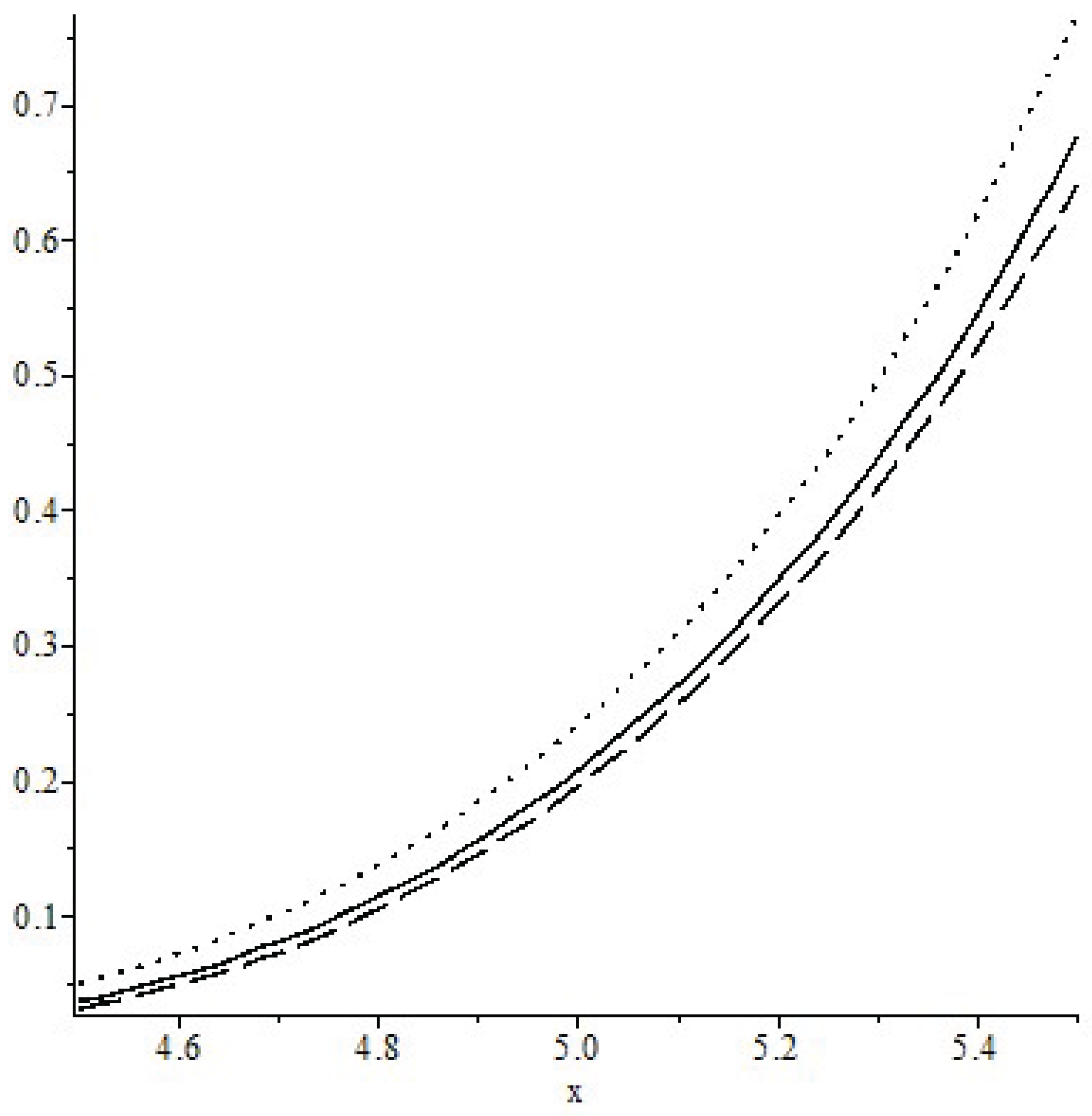
Let us consider the second model of uncertain volatility. Let $\underline{\sigma }=-0.1,\overline{\sigma }=0.2,X_0=0.1,r=0.1,S_0=K=5,T=1.$ The figure shows the graphs of the dependence $\overline{V}(0,x),\underline{V}(0,x)$ and $V(0,x)$ on x, where $\overline{V}(t,x)$ is the solution to problem (6); $\underline{V}(t,x)$ is the solution to problem (8); $V(t,x)$ is the solution to problem (1) for $\sigma =X_0.$ The solid line shows the graph of dependence of $V(t,x)$ on x. The dotted line shows the graph of dependence of $\overline{V}(0,x)$ on x. The dashed line shows the graph of dependence of $\underline{V}(t,x)$ on x.

Figure 1. Graphs of $\overline{V}(0,x),\underline{V}(0,x),V(0,x)$.

Figure 1. Graphs of $\overline{V}(0,x),\underline{V}(0,x),V(0,x)$.

7. Results

This article examines a model of uncertain volatility, a generalization of the well-known Black-Scholes model. Theorems are proven that allow us to estimate the fair price range for an important class of payoff functions. An example of calculating the fair price range for a European call option is given.

8. Discussion

This article is a continuation of [27], which examined two models of uncertain volatility and presented three computational methods for calculating the fair value range of a European-style option. The first method is based on solving the Hamilton-Jacobi-Bellman equations using difference schemes. The second is the Monte Carlo method, which is based on modeling the original stock price process. The third is the tree method, which is based on approximating the original continuous model with a discrete model and obtaining recurrence formulas on a binary tree.

This article proves theorems stating that if the boundary condition is a continuous and convex function, then the solutions to the nonlinear heat equations are convex functions satisfying the linear heat equations. For an important special case, formulas for calculating the fair value range are obtained, which are analogous to the Black-Scholes formula. Calculations using real data are presented, demonstrating the effectiveness of uncertain volatility models compared to the Black-Scholes and Heston models for calculating fair prices for European-style options.

A promising area for future research is the development of a dynamic neural network implementation of uncertain volatility models.

References

- Bachelier, L. Théorie de la spéculation. Annales de l’École Normale Supérieure 1900, 17, 21–86. [Google Scholar] [CrossRef]
- Samuelson, P. Rational theory of warrant pricing. Industrial Management Review 1965, 6, 13–31. [Google Scholar]
- Black, F.; Scholes, M. The pricing of options and corporate liabilities. Journal of Political Economy 1973, 81(3), 637–659. [Google Scholar] [CrossRef]
- Merton, R. Theory of rational option pricing. Bell Journal of Economics and Management Science 1973, 4, 141–183. [Google Scholar] [CrossRef]
- Jacod, J.; Shiryaev, A. N. Limit Theorems for Stochastic Processes; Editor 1, F., Editor 2, A., Eds.; Eizmatlit: Moscow, Russia, 1994; Vol. 1, 2. [Google Scholar]
- Shiryaev, A. N. Fundamentals of Stochastic Financial Mathematics; FAZIS: Moscow, Russia, 2004; p. 512. [Google Scholar]
- Dupire, B. Model Art. RISK Magazine 1993, 6, 118–124. [Google Scholar]
- Dupire, B. Pricing with a smile. RISK Magazine 1994, 7(1), 18–20. [Google Scholar]
- Hull, J. Options, Futures and Other Derivatives, 9th ed.; Prentice Hall: Upper Saddle River, NJ, 2012; p. 432. [Google Scholar]
- Hull, J.; White, A. The pricing of options on assets with stochastic volatilities. Journal of Finance 1997, 42(2), 281–300. [Google Scholar] [CrossRef]
- Johnson, H.; Shanno, D. Option pricing when the variance is changing. Journal of Financial and Quantitative Analysis 1987, 22(2), 143–151. [Google Scholar] [CrossRef]
- Stein, E.; Stein, J. Stock price distributions with stochastic volatility: an analytic approach. Review of Financial Studies 1991, 4(4), 727–752. [Google Scholar] [CrossRef]
- Scott, L. Option pricing when the variance changes randomly. Theory, estimation and an application. Journal of Financial and Quantitative Analysis 1987, 22(4), 419–438. [Google Scholar] [CrossRef]
- Heston, S. A closed-form solution for options with stochastic volatility with applications to bond and currency options. The Review of Financial Studies 1993, 6(2), 327–343. [Google Scholar] [CrossRef]
- Vellekogp, M.; Nieuwenhuis, J. A tree-based method to price American options in the Heston model. The Journal of Computational Finance 2009, 13(1), 1–21. [Google Scholar] [CrossRef]
- Briani, D.; Caramellino, L.; Zanette, A. A hybrid approach for the implementation of the Heston model. IMA Journal of Management Mathematics 2017, 4, 467–500. [Google Scholar] [CrossRef]
- Alfonsi, A. High order discretization schemes for the CIR process: application to affine term structure and Heston models. Mathematics of Computation 2010, 79, 209–237. [Google Scholar] [CrossRef]
- Luzhetskaya, P. A.; Kudryavtsev, O. E. Computation of option prices in stochastic volatility models. Engineering Journal of Don 2020, 5. [Google Scholar]
- Rouah, F.; Steven, L. The Heston Model and Its Extensions in Matlab and C; John Wiley and Sons: Hoboken, New Jersey, 2013; p. 411. [Google Scholar]
- Danilova, N. V.; Kudryavtsev, O. E. Computation of option prices in the Heston model using artificial neural networks. University News. North-Caucasian Region. Natural Sciences 2024, 4, 31–37. [Google Scholar]
- Kahl, C.; Jackel, P. Not so-complex logarithms in the Heston model. Wilmott 2005.
- Belyavsky, G. I.; Danilova, N. V. Calculation of the fair price of a European option in a (B,S)-market model with a barrier based on a random walk. University News. North-Caucasian Region. Natural Sciences 2015, 4, 25–28. [Google Scholar]
- Belyavsky, G. I.; Danilova, N. V. Calculation of the fair price of a barrier option in a (B,S)-market model with parameter switching. University News. North-Caucasian Region, Natural Sciences 2016, 1, 11–16. [Google Scholar]
- Belyavsky, G.; Danilova, N.; Zemlyakova, I. Optimal control problems with disorder. Automation and Remote Control 2019, 80(8), 1419–1427. [Google Scholar] [CrossRef]
- Belyavsky, G.; Danilova, N.; Zemlyakova, I. Optimal control in binary models with the disorder. Engineering Letters 2021, 29(4), 1359–1364. [Google Scholar]
- Belyavsky, G. I.; Danilova, N. V. Control in binary models with disorder. Bulletin of the South Ural State University. Series: Mathematical Modelling, Programming and Computer Software, 2022; 15, 3, 67–82. [Google Scholar]
- Belyavsky, G. I.; Danilova, N. V. Models with uncertain volatility. Bulletin of the South Ural State University. Series: Mathematical Modelling, Programming and Computer Software, 2023; 16, 3, 5–19. [Google Scholar]
- Avellaneda, M.; Levy, A.; Paras, A. Pricing and hedging derivative securities in markets with uncertain volatilities. Applied Mathematical Finance 1995, 2, 73–88. [Google Scholar] [CrossRef]
- Peng, S. G-Brownian Motion and Dynamic Risk Measure under Volatility Uncertainty 2007.
- Shiryaev, A. N. Brownian Motion; Vol. 2; 2025; pp 576–603.
- Schiesser, W.; Griffiths, G. A Compendium of Partial Differential Equation Models: Method of Lines Analysis with Matlab; Cambridge University Press: Cambridge, 2009; p. 491. [Google Scholar]
- Crandall, M.; Ishii, H.; Lions, P. User’s guide to viscosity solutions of second order partial differential equations. Bulletin of the American Mathematical Society 1992, 27(1), 1–67. [Google Scholar] [CrossRef]
- Barles, G.; Souganidis, P. Convergence of approximation schemes for fully nonlinear second order equations. Asymptotic Analysis 1991, 4, 271–283. [Google Scholar] [CrossRef]
- Robin Dunn. Estimating Option Prices with Heston’s Stochastic Volatility Model. Available online: https://www.valpo.edu/mathematics-statistics/files/2015/07/Estimating-Option-Priceswith-Heston (accessed on 16 September 2025).
Disclaimer/Publisher’s Note: The statements, opinions and data contained in all publications are solely those of the individual author(s) and contributor(s) and not of MDPI and/or the editor(s). MDPI and/or the editor(s) disclaim responsibility for any injury to people or property resulting from any ideas, methods, instructions or products referred to in the content. |
© 2025 by the authors. Licensee MDPI, Basel, Switzerland. This article is an open access article distributed under the terms and conditions of the Creative Commons Attribution (CC BY) license (http://creativecommons.org/licenses/by/4.0/).
Copyright: This open access article is published under a Creative Commons CC BY 4.0 license, which permit the free download, distribution, and reuse, provided that the author and preprint are cited in any reuse.