Submitted:
29 October 2025
Posted:
29 October 2025
You are already at the latest version
Abstract
This work presents solutions to the strongly coupled nonlinear Wilberforce pendulum model. We begin by presenting three specific cases of the equations of motion of the nonlinear Wilberforce Lagrangian. We find solutions governed by Jacobi elliptic functions, Mathieu functions, Weierstrass elliptic functions and obtaining beating behavior of plane waves when their frequencies are close and the phase is proportional to their amplitudes. Similarly, we find analytical solutions showing the power of these methods using the tanh, Riccati, Jacobi, and generalized Jacobi solitary wave solution techniques, without any restrictions.
Keywords:
Wilberforce pendulum
; Jacobi elliptic functions
; Mathieu equation
; Weierstrass elliptic functions
; solitary wave methods
1. Introduction
The Wilberforce pendulum is a mechanical device that ingeniously couples the translational and rotational degrees of freedom of a non-point mass attached to a spring [1]. The mass undergoes two motions: the first is vertical, driven by the spring’s translational restoring force, and the second is rotational around the axis of translation, also due to the spring’s torsional properties [2,3]. Basically, spring stretches and contracts vertically, and twists and untwists around that same translational axis. British physicist Lionel Robert Wilberforce invented it and published his findings in 1896 [1].
Newton’s second law, Hamiltonian, or Lagrangian dynamics can describe this device’s physical behavior [4,5,6,7]. If we work with the latter, we can clearly postulate how the coupling terms appear in the dynamical system and how they impact the laws that describe the device [5,6,7]. This approach from classical mechanics has two approximations: one linear and the other nonlinear. In scenario one, the linear coupling term is ϵyθ. Here, ϵ represents a phenomenological coupling constant that determines the strength of the nonlinear interaction, y refers to the translational coordinate, and θ describes rotational motion [5,6,7]. These terms, together with the kinetic and potential energy of each element of the system, generate a pair of coupled linear equations, whose key prediction is the emergence of beat-like behavior between the translational and rotational coordinates. In the second scenario, the reference's nonlinearity is proportional to ϵ(yθ)2 and can be modeled as a perturbative term describing the system’s phase-space structure [7].
On the other hand, in recent decades new analytical methods, called solitary wave methods, have emerged to tackle the difficult and very arduous task of obtaining analytical solutions to nonlinear ordinary or partial differential equations. Among these new methods, we can mention the highly important work of W. Malfliet, in which a very insightful strategy is devised to express the solution in terms of solitary waves, offering the advantage that the solution to a given differential equation can be established as a finite sum of hyperbolic tangent terms and their derivatives [8]. Similarly, alternative approaches exist, like those using Riccati equation solutions, which build on Malfliet’s idea by representing the desired solution as a finite sum of Riccati solutions [9]. Auxiliary differential equations yield multiple solution families, each as a finite sum satisfying the equation. Solitary wave methods improved by applying Jacobi elliptic functions. When we set combinations of analytical solutions of the Jacobi differential equation [reference], this drives a significant deep insight into the number of solutions discovered. This improved solitary wave technique now provides advanced solutions for Klein–Gordon equations with quadratic perturbations. This study aims to employ solitary wave methods in analyzing the Wilberforce nonlinear oscillation system. Finally, we present additional results for certain cases given by Jacobi elliptic and Mathieu functions that enlighten how this complex nonlinear oscillator behaves.
2. The Lagrangian Model
A lagrangian that gives into accounts the nonlinear coupling in the system is [7]:
The nonlinear equations are.
With, and and . Where is the moment of inertia, m the mass, is the spring constant, is the rotational spring constant, and is the term that accounts for the coupling between the rotational and translational degrees of freedom.
3. Approximate Solutions
3.1. Specific Case: ,
If we assume that ,
This equation becomes a solution of the harmonic oscillator.
Substituting into Equation (2)
Using ,
Defining
The solution is.
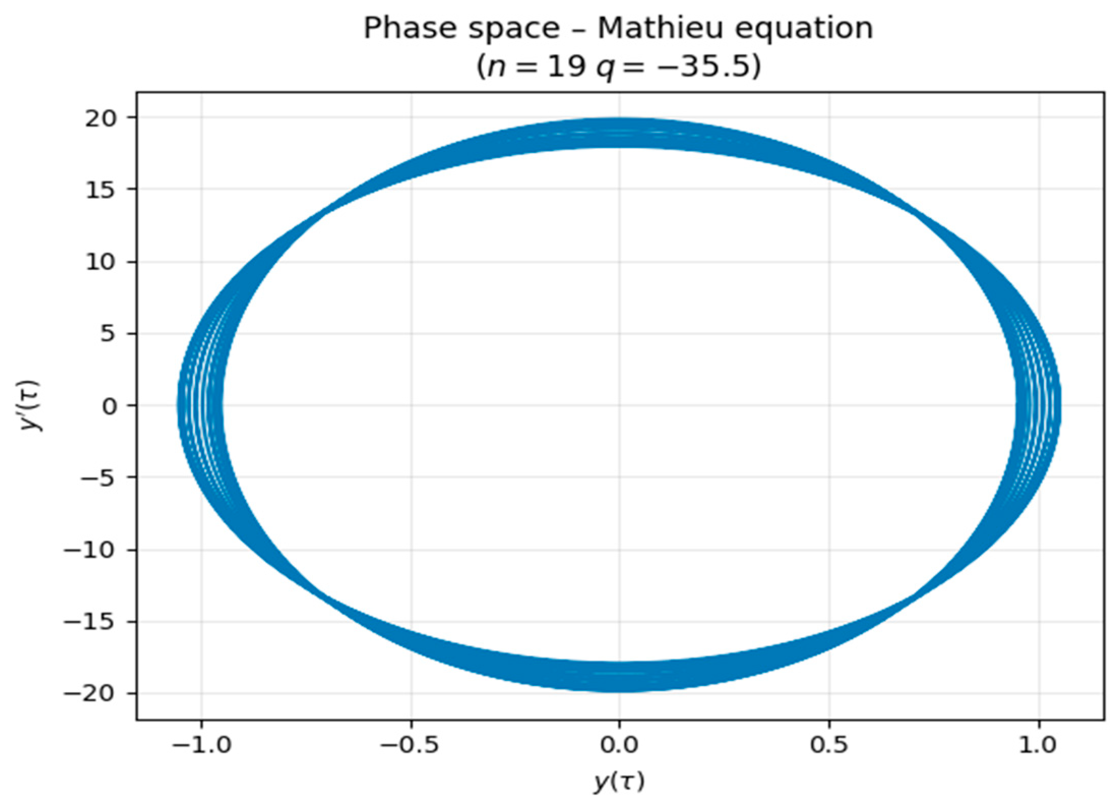
where, and are constants determined from initial condition, and is the even periodic Mathieu functions and are the odd Mathieu functions and is an integer indexing the characteristic values.
Figure 1.
Phase space, mass m=1, Equation (10).
3.2. Specific Case:
Also, we have the case where equal frequencies, we suppose a proportional solution having as a constant. So, the system of equations (2) and (3) reduce to
The system reduces to the Duffing equation [10].
3.3. Specific Case: Complex Solutions
Also, we postulate solutions [4], given by
Replacing in Equation (2-3)
The frequencies of the normal modes are.
A general solution is:
Taking initial conditions as and
And doing
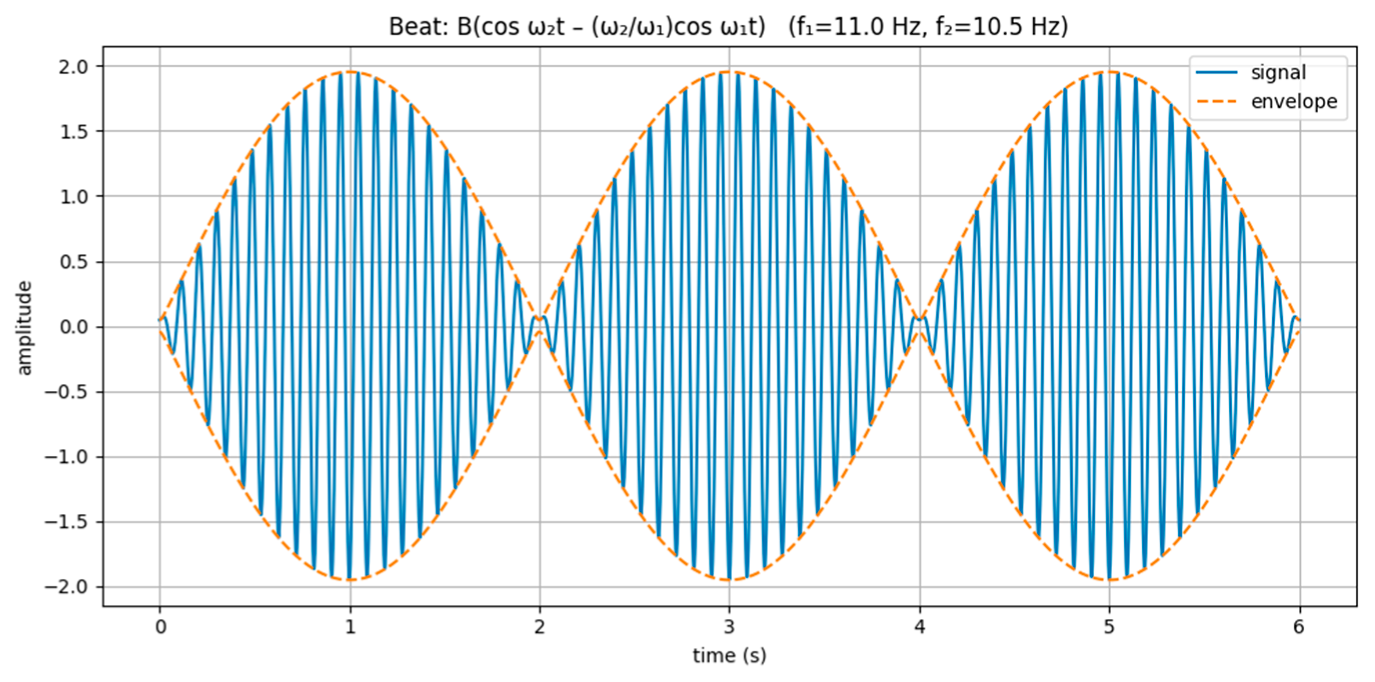
Figure 1.
Beating behavior Equation (21).
3.4. Specific Case:
,
In the same way we suppose solution given by having as a constant. Therefore, equations (2) and (3) become:
Using
Equation (22) is.
The integrating factor is ,
Defining is ,
Which is the Weierstrass Elliptic differential equation
And Weierstrass elliptic function. If we want to deplete the quadratic term in equation (26), we define.
where and are parameters. Defining , and in equation (23), . We obtain.
Then, the solution is.
4. Solitary Wave Solutions
4.1. Tanh Solitary Wave Method
We use the Tanh solitary wave method [12], where the solution is:
The derivatives of , are.
Replacing in equations (2)-(3):
Now, balancing the highest-order linear derivative with the highest order nonlinear terms in equations (25)-(26):
Therefore
Their derivatives are.
Replacing in equations (25)-(26):
Then, we get a set of equations, order by order in . Applying algebra yields:
So, the solutions are.
Then, equations (35)-(38) determine , and .
4.2. Riccati Solitary Wave Method
Here and are constants, Table 1. Again, balancing nonlinear terms in equations (1)-(2), We have m=1, n = 1. Therefore, the solutions and their derivatives are:

Table 1.
List of solutions to equation (42).
| F | ||
|---|---|---|
| 1/2 | -1/2 | coth(t) ±cosh(t), tanh(t), ±isech(t) |
| 1/2 | 1/2 | sec(t) ± itan(t), |
| -1/2 | -1/2 | csc(t) ± icot(t), |
| 1 | -1 | coth(t), tanh(t), |
| 1 | 1 | tan(t), |
| -1 | -1 | cot(t), |
Replacing in equations (2)-(3)
We obtain a set of algebraic equations and solving them, we get a set of family’s solutions.
where , represents a complex number. The solutions are:
Table 1 lists the solutions for F.
4.3. Soliton Solitary Wave Method
And , and are parameters, and J the solution. Again, balancing
nonlinear terms in equations (2)-(3), we have m=1, n = 1. Then, equations (53) are:
Then, equations (54) are:
Again, we get a set of equations, order by order in , and by doing algebra, we get:
Table 1.
List of solutions to equation (55).
| T | ||||
|---|---|---|---|---|
| -1 | 1 | 1 | sn() | |
| -1 | 1 | cn(), | ||
| -1 | 1 | 1 | dn(), | |
| -1 | 1 | 1 | cd(), | |
| 1 | 1 | sd(), | ||
| 1 | -1 | 1 | nd(), | |
| 1 | 1 | -1 | dc(), | |
| 1 | -1 | nc(), | ||
| 1 | 1 | 1 | sc(), | |
| 1 | 1 | -1 | ns(), | |
| 1 | 1 | ds() | ||
| 1 | 1 | 1 | cs(), |
4.4. Elliptic Solitary Wave Method 1
And a, b, c and are parameters, and T the solution (referencia Jacobi). Again, balancing nonlinear terms in equations (1)-(2), we have r=1, s = 1, in summations (46). Then
Therefore
The movement equations (1)-(2) are:
Then, we obtain a group of coupled equations, order by order in . After performing algebraic operations, the result is as follows:
For all the six families of solutions . So, the solutions are:
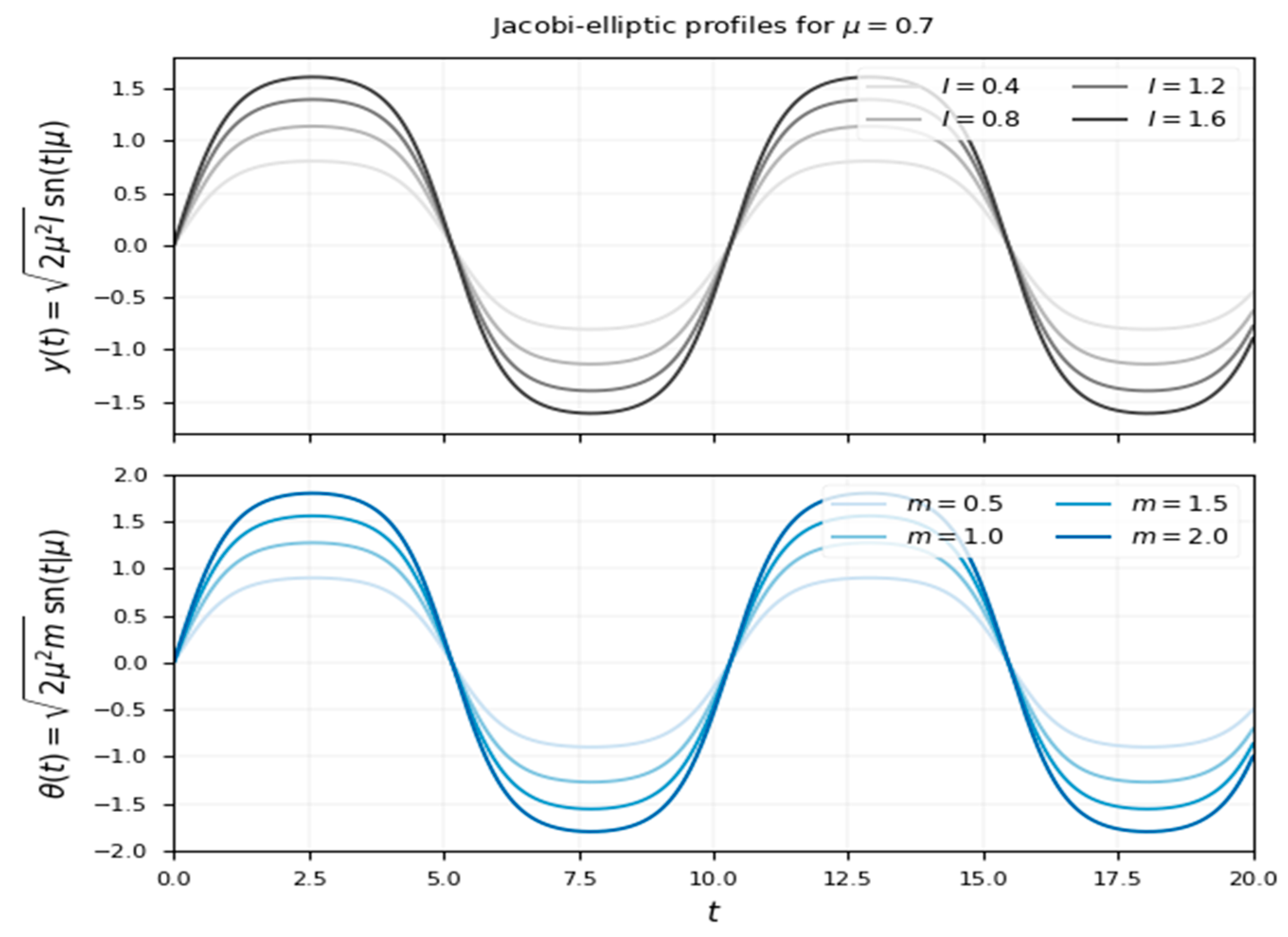
To show the result, we apply the first row that defines the solution of sn Jacobi elliptic function in table (1), and the conditions exposed in the family of solutions
And now
Figure 2.
Jacobi elliptic function solution sn.
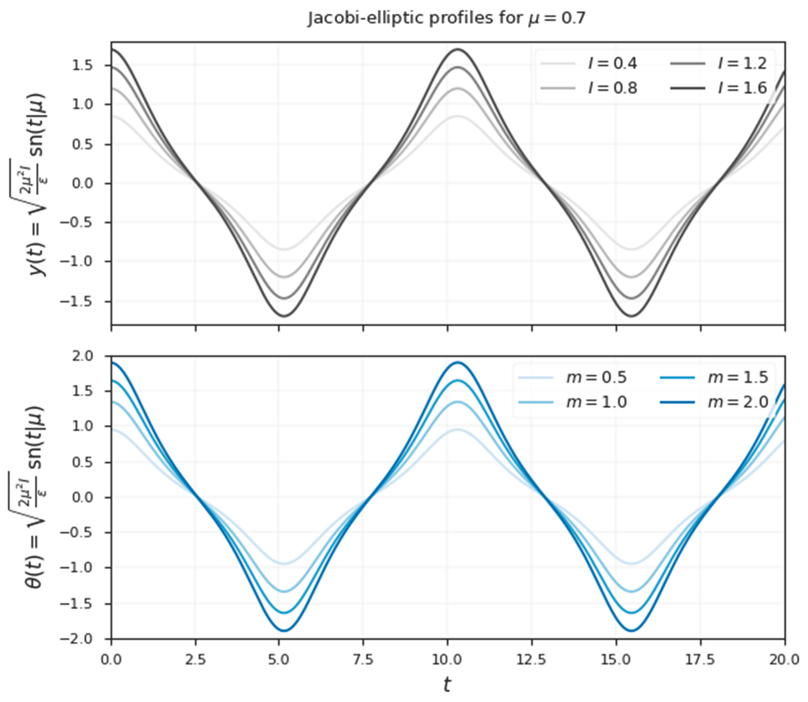
Following with results, we apply the second row that defines the solution of cn Jacobi elliptic function in table (1), and the conditions exposed in the family of solutions
And now
Figure 3.
Jacobi elliptic function sn governing and .
4.5. Elliptic Solitary Wave Method 2
And a, b and are parameters, and G the solution. Again, balancing nonlinear terms in equations (2)-(3), so m=1, n = 1. Then, equations (54) are:
Then, equations (54) are:
Then, we get a set of equations, order by order in , and by doing some algebra, we get:
5. Conclusions
Extending the linear Wilberforce pendulum to the nonlinear system poses a complex analytical problem, and to date no analytical solution is known. When we consider special cases—parameter-space restrictions that define the equations of motion—we find approximate equations such as the Duffing equation, the Mathieu equation and Weierstrass elliptic differential equation; similarly, by assuming complex exponential solutions, we observe beating behavior when frequencies are close. Given these perspectives on the complexity of the problem, we turn to novel and up-to-date analytical tools that have proven their worth in various fields of physics and are known as solitary wave solutions. For the problem under consideration, we have applied the tanh method, one of the original methods, Riccati solutions, and two tools based on Jacobi function solutions. We have found a respectable number of solutions demonstrating the method’s capabilities. In this same vein, new types of couplings between rotational and translational variables can be designed to reflect internal geometric symmetries in the system’s Lagrangian—for example, invariance under coordinate exchange, under multiplication of the degrees of freedom by a complex phase, or under rotations in the internal coordinate space.
Funding
This research was funded by Universidad Nacional de Colombia through Hermes Project 64072 and sabbatical year under resolution 2445 of the Faculty of Sciences Universidad Nacional de Colombia, September 27, 2024.
Conflicts of Interest
The author declares no conflicts of interest.
References
- L.R. Wilberforce M.A. On the vibrations of a loaded spiral spring. Philosophical Magazine Series 1894, 38, 386–392. [CrossRef]
- R.E. Berg and T.S. Marshall. Wilberforce pendulum oscillations and normal modes. Am. J. Phys 1991, 59, 32–38. [CrossRef]
- F.G. Karioris. Wilberforce pendulum, demonstration size. Am. J. Phys 1993, 31, 314–315. [CrossRef]
- J.R. Taylor. Classical Mechanics, 1a ed.; University Science Books: Sausalito California, EE.UU. 2005; pp. 237–281.
- V. Dos P. de Souza, P. Gonçalves and E. Marinho Jr. Experimental study of coupled oscillations on a Slinky Wilberforce pendulum. Revista Brasileira de Ensino de Física 2022, 44, e20220037. [CrossRef]
- M. Plavcic and P. Zupanovic. The resonance of the Wilberforce pendulum and the period of beats. Lat. Am. J. Phys. Educ. 2009, 3, 8. [CrossRef]
- M. Avendaño-Camacho, A. Torres-Manotas and J.A. Vallejo. Closed stable orbits in a strongly coupled resonant Wilberforce pendulum. Journal of Vibration and Control. 2021, 0, 1–10. [CrossRef]
- M. Abramowitz and I.A. Stegun. Handbook of Mathematical Functions with Formulas, Graphs, and Mathematical Tables, 1a ed.; Dover Publications Inc.: New York, EE.UU. 1965; pp. 721–746.
- L. Rubi. Applications of the Mathieu equation. Am. J. Phys. 1996, 64, 39–44. [CrossRef]
- W.P. Reinhardt and P.L. Walker. Digital Library of Mathematical Functions. Chapter 22 Jacobian Elliptic Functions. URL https://dlmf.nist.gov/22.
- W. Malfliet. Solitary wave solutions of nonlinear wave equations. Am. J. Phys. 1992, 60, 650–654. [CrossRef]
- H. Salas, J. E. Castillo, and J.E. Pinzon. Solution of Duffing’s differential equation by means of elementary functions and its application to anon-linear electrical circuit. International Journal of Mathematics and Computer Science. 2022, 17, 277–287. http://ijmcs.future-in-tech.net.
- E.S. Fahmy, K.R. Raslan and H.A. Abdusalam. On the exact and numerical solution of the time-delayed Burgers equation. International Journal of Computer Mathematics. 2008, 85, 1637–1648. [CrossRef]
- H. Almusawa and A. Jhangeer. A Study of the Soliton Solutions with an Intrinsic Fractional Discrete Nonlinear Electrical Transmission Line. Fractal Fract. 2022, 6, 334. [CrossRef]
- M. Inc and M. Ergüt. Periodic wave solutions for the generalized shallow water wave equation by the improved Jacobi elliptic function method. Applied Mathematic E-Notes. 2005, 5, 89–96. http://eudml.org/doc/51264.
- S. A. Madani et. al. Exploring novel solitary wave phenomena in Klein-Gordon equation using ϕ6 model expansion method. Sci Rep. 2025, 15, 1834. [CrossRef] [PubMed]
- G. Pastras. Four Lectures on Weierstrass Elliptic Function and Applications in Classical and Quantum Mechanics. arXiv 2017, arXiv:1706.07371v2. [math-ph] 6.
- Yum-Tong Siu, Advanced Complex Analysis. Available online: https://people.math.harvard.edu/~siu/math213a/elliptic_function_weierstrass_approach.pdf (accessed on 24 October 2025).
- E.A. Saied, Reda G. Abd El-Rahman, Marwa I. Ghonamy. A generalized Weierstrass elliptic function method for solving some nonlinear partial differential equations. Computers and Mathematics with Applications. 2009, 58, 1725–1735. [CrossRef]
Disclaimer/Publisher’s Note: The statements, opinions and data contained in all publications are solely those of the individual author(s) and contributor(s) and not of MDPI and/or the editor(s). MDPI and/or the editor(s) disclaim responsibility for any injury to people or property resulting from any ideas, methods, instructions or products referred to in the content. |
© 2025 by the authors. Licensee MDPI, Basel, Switzerland. This article is an open access article distributed under the terms and conditions of the Creative Commons Attribution (CC BY) license (http://creativecommons.org/licenses/by/4.0/).
Copyright: This open access article is published under a Creative Commons CC BY 4.0 license, which permit the free download, distribution, and reuse, provided that the author and preprint are cited in any reuse.


