
Submitted:
27 October 2025
Posted:
29 October 2025
You are already at the latest version
Abstract
To improve the classification accuracy about K-means model for Coal-Gangue-Image, this paper proposed an Coal-Gangue-Image Classification Method (AF-WPOA-Kmeans-CCM) based on K-means and an improved wolf-pack-optimization using Adaptive Adjustment Factor.Firstly, this paper proposed an improved wolf-pack-optimization algorithm(AF-WPOA) using Adaptive Adjustment Factor Strategy(AF) aimed to dynamically adjust the update amount of the population for maintaining the genetic diversity of the population while accelerating convergence speed as well as ASGS devoted to enhance the algorithm's global exploration capability in hunting mechanism and local exploitation power in siege mechanism.Secondly,different weights for each feature dimension were adopted to more accurately reflect the varying importance of different feature dimensions in the classification results while Hilbert space was used to eliminate the drawback of low feature dimensions of the images from this paper resulted to achieving higher classification accuracy in high-dimensional space.Finally,AF-WPOA-Kmeans-CCM was formed by adopting the AF-WOPA to optimize K-means clustering model dedicated to accurate classification of Coal-Gangue-Image. Experimental results show that AF-WPOA outperforms GA, PSO and LWCA, while AF-WPOA-Kmeans-CCM performs better than Kmeans-CCM, GA-Kmeans-CCM, PSO-Kmeans-CCM, and LWCA-Kmeans-CCM—achieving 93.03% and 91.55% classification ac-curacy on the training and testing sets, respectively. Unfortunately, Coal-Gangue-Image often have diverse sources and significant feature differences. This makes it hard for fixed cluster centers to fully represent the numerous, multi-source, and highly variable unknown samples to be predicted.
Keywords:
coal-gangue
; image classification
; Wolf Pack
; K-means
1. Introduction
The K-means clustering model has many advantages such as simple principle, easy to implement, fast convergence speed, good clustering effect, and easy to interpret and understand. Recently, many applications and researches about image-classification of K-means clustering have been done, such as authors used PSO-optimized Kmeans clustering for image segmentation in paper [1]; Zhou Xiang et al. applied the K-means clustering method for mechanical condition monitoring in paper [2]; Authors employed the K-means clustering combined with support vector machine method for the classification of hyperspectral images [3];Zhou Zhixiang et al. used a shallow fuzzy K-means clustering method to obtain the centers of each cluster to construct the image feature vector, the method is innovative while the steps are relatively complex and the classification accuracy is not good enough [4];Authors adopted an improved K-means algorithm for object detection in the field of transportation [5];El Far et al. employed the K-means clustering method for 3D target retrieval [6];Jaisakthi, Seetharani et al. deployed the K-means method for automated segmentation of dermatological images to assist in the diagnosis of skin lesions [7];Authors employed the K-means method to address the image classification problem of Polarimetric Synthetic Aperture Radar (PolSAR) and proposed an unsupervised K-means algorithm based on random distances for PolSAR area classification [8]; Researchers have proposed a K-means clustering algorithm based on a weighted visual dictionary, which is excellent in descriptive image information and can provide image classification performance, however, establishing a visual dictionary is meaningless and wastes computational resources for the classification problem of image waste rock with only a few categories [9]; Chen Guilin et al. employed the K-means method to assist neural networks in improving the accuracy of image classification in the presence of interference noise [10];Writers adopted a color feature-based K-means method for remote sensing image classification, and it is clear that this method is not suitable for image gangue classification with insufficient color features [11];L. Ke et al. proposed a remote sensing image classification method based on superpixels and adaptive weighted K-means. The calculation of this adaptive weighting method takes into account the color space and coordinate position of the pixels, and is not suitable for classifying images with insufficient color information [12]; K-means method is also devoted to image classification in different fields, but the above image classification methods based on K-means have shortcomings, especially for image gangue classification, which is not applicable [13,14,15].
K-means clustering model can be used for coal-gangue-image classification.However, the classification model based on minimum distance is prone to getting stuck in local optima, especially in the complex production environment of coal mines where coal-gangue-images are generated, characterized by high noise that is difficult to avoid and relatively low feature dimensions, leading to a low classification accuracy of the K-means model for coal gangue.The fundamental issue lies in that classification model based on original K-means randomly selects initial cluster centers introducing uncertainty, and continuously adjusts each cluster center dynamically resulting to consuming substantial computational resources as well as it treats each feature dimension equally without considering the different importance of each feature dimension to the classification results during the clustering process.
Accordingly, this paper proposes a Coal-Gangue-Image Classification Method (AF-WPOA-Kmeans-CCM) based on K-means and an improved wolf-pack-optimization using Adaptive Adjustment Factor. Firstly, an improved wolf-pack-optimization algorithm(AF-WPOA) inspired by the Wolf colony search algorithm based on leader strategy(LWCA) in [16] are proposed with Adaptive Adjustment Factor Strategy(AF) aimed to dynamically adjust the update amount of the population for maintaining the genetic diversity of the population and accelerate convergence speed as well as ASGS devoted to enhance the algorithm’s global exploration power in hunting mechanism and local exploitation power in siege mechanism. Secondly, different weights for each feature dimension were adopted to more accurately reflect the varying importance of different feature dimensions in the classification results while Hilbert space was used to eliminate the drawback of low feature dimensions of the images from this paper resulted to achieving higher classification accuracy in high-dimensional space. Finally, AF-WPOA-Kmeans-CCM was formed by adopting the AF-WOPA to optimize K-means clustering model dedicated to accurate classification of Coal-Gangue-Image.
2. Related Works
2.1. Wolf-Pack-Optimization Algorithm
The wolf pack optimization algorithm(WPOA) is inspired from hunting of wolf-pack in nature, and it abstracts the Migration- Mechanism, Summon-Raid-Mechanism,Siege-Mechanism,and Updating-Mechanism from wolves-hunting produre,so as to evolve into a new swarm intelligence optimization algorithm.
It can be assumed that the foraging and hunting space (or problem domain) of the wolf pack is a Euclidean space of N×D [17], where N is the number of wolf populations and D is the number of variables or dimensions to be optimized. The position state of the i-th wolf in the wolf pack can be expressed as Xi = (xi1 ,xi2 ,... ,xiD), where xid represents the position or coordinate value of the i-th wolf in the variable space of the d (d =1,2 ,... ,D) dimension in the solution space; The prey odor concentration perceived by the wolf is Y=f(X), where Y is the objective function value. The distance between p and q of any two wolves is defined as the Manhatan distance between their state vectors [18].
In this paper, the number of wolves is expressed by N, and the number of dimensions of the search space or solution space is expressed by D, and the location of the i-th wolf is obtained by Equation (1)
Among them, xid represents the position of the i-th wolf in the d-th dimension; N represents the number of wolves in the population; D is the number of dimensions in the solution space.
Initialization. The initial position of each wolf in the population can be obtained from Equation (2).
Rand(0,1) is a random number uniformly distributed over the interval [0,1]; RANGEmax and RANGEmin are the upper and lower limits of the solution space,detailed in paper [16].
2.1.1. Migration Mechanism
Based on paper [19],each wolve in the pack can be the leader one of the pack upon its own fitness and the ones of the pack, that is, if the fitness of one wolf is the best in the pack, then this one will be the leader of the pack, and Equation (3) shows the migration way to calculate the new location of i-th wolf in the d-dimensional space.
Unfortunately, as an abstract optimization algorithm rather than a specific biological process, the description of the migration and Equation (3) is too complex. in paper [20], the ‘hunting’ Equationhas been simplified and improved to Equation (4).
Among them, Pkjd is the position of the j-th wolf in the d-th dimension while searching in the k-th search direction, and wjd is the original position of the j-th wolf in the d-th dimension; stepa1 is the adaptive step size; Chaos(-1,1) is a chaotic variable uniformly distributed in the interval [-1,1], produced by Equation (5).
In paper [16], the Equationfor ‘hunting and gathering’ is described as Equation (6).
Among them, yid represents the position of the j-th point in the d-th dimension among the h points generated near the competing wolf; Rand is a random number uniformly distributed in the interval [-1, 1]; xxid is the current position of the i-th competing wolf in the d-th dimension; stepa is the step length of the search.
There are differences between these Equations, but they all follow the basic process of wolf pack hunting behavior, with differences in their operating mechanisms. It is these differences that continuously drive the improvement of the wolf pack optimization algorithm.
2.1.2. Summon-Raid Mechanism
According to the concepts in paper [16], in this step, once the pack receives the call signal from the lead wolf, they all move towards the lead wolf and update their positions on the way to the ambush based on Equation (7). If the new position provides a better fitness value than the current one, the wolf will move to the new position; otherwise, it will remain in its current location.
Among them, zid represents the updated position of the i-th wolf in the d-th dimension within the wolf pack; xid is the current position of the i-th wolf in the d-th dimension; Rand is a random number uniformly distributed in the interval [-1,1]; stepb is the summon-chase step length; xld is the position of the leader wolf or alpha wolf in the d-th dimension.
In Equation (7), theoretically, the larger the stepb, the faster the wolf pack approaches the wolf (the lead wolf) currently making the howling sound. The benefit of this is to accelerate the convergence speed of the algorithm, allowing it to converge quickly.
2.1.3. Siege Mechanism
According to the ideas in paper [16], for this produre, a random number rm is first generated within the range of [0,1]. If rm is less than θ (which is a pre-set threshold), the i-th wolf does not move; if rm is greater than θ, the i-th wolf surrounds the prey centered around the leader wolf. The updated wolf position can be determined by Equation (8).
stepc is the encircling step length; Xl is the position of the leader wolf; is the current position of the i-th wolf in the t-th generation.
In order to obtain the global optimal solution to the optimization problem, it is hoped that in the early stages of the algorithm’s iteration, the attack step or surrounding step should be set larger, so as to explore the optimal solution in a broader area. Conversely, in the later stages of the algorithm’s iteration, as the current solution approaches the theoretical optimal solution, it is hoped that the attack step or surrounding step diminishes with an increase in the number of iterations, allowing the algorithm to finely search for the optimal solution in a smaller area, thereby increasing the likelihood of finding the global optimal solution. The attack step stepc can be obtained using Equation (9).
Here, t represents the current iteration count; T represents the maximum iteration count allowed for the algorithm; stepcmax and stepcmin are the upper and lower limits of the assault step size.
2.1.4. Updating of Population
According to the ideas in paper [16], the specific operation is to remove the worst m (a fixed integer) wolves, and then randomly generate an equal number of m wolves, ensuring that new genes are continuously injected into the population and that the population size remains stable, thus avoiding the algorithm getting stuck in local optima.
However, the variable m is a fixed number and can not react the need of pratical issues or engineerings. Therefore, the update amount of the population in the WPOA algorithm should be changed based on dynamic variables specific to the problem. According to the ideas in paper [19], the population update amount m is chosen as a random integer between [N/(2×β), N/β], where N is the population size of the wolves and β is the proportion factor for population updates.。
2.2. ASGS
The Strategy of Adaptive Shrinking Grid Search (ASGS) requires each wolf responsible for exploration to search in different directions within a D-dimensional solution space.
Based on traditional ideas and the wolf pack algorithms such as CWOA, during the migration process, each wolf only performs a limited number (h) of searches around itself (with h being less than the dimensionality D of the solution space). Figure 1a shows the original schematic about hunting and attacking while Figure 1b shows the one of ASGS Strategy. Here,the red points represent the coordinates of current wolf and the black ones indicate the next possible positions that the wolf will move to.
According to the pricinple of ASGS, an adaptive grid with (2×K + 1)D nodes centered the current wolf are generated along the 2×D direction, detailed in Equation (10) and refor to paper [21].
According to the concept of the ASGS strategy, a node in the grid can be obtained based on Equation (11). In the Equation, the step can be either the hunting step length stepa or the siege step length stepc, the calculation of which is provided by Equation (12).
At the end of each migration process, by comparing the goodness of the fitness values, the leader wolf or alpha wolf of the pack is determined. It should be particularly noted that as the hunting step size or siege step size continues to decrease, the adaptive grid in the adaptive shrinking grid search strategy will also continue to shrink. Clearly, compared to traditional methods that examine a single isolated point, examining (2×K + 1)D points centered on the current position based on the adaptive shrinking grid search strategy increases the accuracy of the search and the likelihood of discovering local and global optima.
In the same way, during the siege process, the same strategy is applied, with the difference that the siege step length stepc is smaller than the hunting step length stepa. At the end of each siege process, by comparing the fitness values, the head wolf or leading wolf of the pack is determined.
2.3. K-Means
K-means clustering algorithm is a dynamic clustering method. The characteristic of dynamic clustering is that it requires determining a criterion function to evaluate the quality of the clustering results, giving an initial classification, and then using an iterative algorithm to find the best clustering result that makes the criterion function take the extreme value. The construction principle of the K-means clustering algorithm model is as follows: first, m sample points are arbitrarily selected from n samples as the initial clustering center; for the remaining samples, they are assigned to the cluster with the most similar (represented by the clustering center) according to their similarity (distance) to these clustering centers; then the clustering center (the mean of all objects in the cluster) is calculated for each new cluster; this process is repeated until the standard measure function converges. k-means clustering takes the minimum sum of squares of distances as the criterion function.
Input: sample set to be clustered D ={x1,x2,…,xM},number of clusters K, maximum number of generations n.
Output: clustered cluster C = { C1,C2,...,CK }.
As shown in Figure 2, the steps are as follows:
Step 1: K clustering centers are randomly selected from dataset D, and the corresponding vectors are (μ1,μ2,…, μK).
Step 2: Calculate the distance -ull from each sample point to K clustering centers, and classify each sample point into the cluster closest to it.
Step 3: Recalculate the center vector μk of K clusters obtained in step 2 and use it as the new clustering center.
Step 4: Repeat steps 2 and 3 until the maximum number of iterations n is met or the center vector of all clusters no longer changes, and the clustered clusters are output C ={ C1,C2,…,CK }.
3. Improvement
To further improve the optimization capability of WPOA and enhance the classification accuracy of Coal Gangue image, this paper proposes the following two strategies.
3.1. Adaptive Adjusted Factor Strategy(AF)
In the early stages of the iteration process of the wolf pack optimization algorithm, there is often a desire for the algorithm to optimize over a large range, which means strengthening the global exploration capability as much as possible. This requires more genetic diversity within the population, meaning: the population update amount should be relatively large. As the iteration process advances, individuals in the algorithm are likely to converge towards potential optimal solutions; at this point, it is desirable to gather more individuals to enhance the algorithm’s local exploitation power, which does not require too much genetic diversity in the population because excessive genetic diversity can affect the convergence speed of individuals and even cause the algorithm to diverge, meaning: at this time, the population update amount should be relatively small. In the later stages of the algorithm’s iteration, individuals in the population are generally stabilized around their respective local optimal solutions (including potential global optimal solutions); at this time, appropriately increasing the population update amount can help the algorithm escape from local optima.
Based on the above analysis, a dynamically changing population update amount can be derived, as given by Equation (14).
Among them, AF is the adaptive factor; t is the current iteration number; T is the maximum iteration number; Regeration_Num is the adaptive dynamic population update amount; floor is a function that rounds down the given value.
3.2. K-means Clustering with Weight Factors
The principle of the K-means clustering model can be used for coal-gangue-image classification, the principle is to randomly select K samples as the initial classification center, calculate the distance from the unknown samples to be tested to each cluster center, determine the attribution category of the new samples to be tested at the minimum distance, and then dynamically adjust each cluster center to determine the attribution category of the next unknown sample to be tested, and iterate multiple times until all the samples to be tested are labeled and classified. However, the K-means clustering model based on the minimum distance to determine the classification category is easy to fall into the local optimum, especially in the face of the characteristics of large noise and difficult to avoid and low feature dimension of the coal-gangue-image sample data generated in the complex production environment of coal mines, which makes the classification accuracy of the K-means clustering model not high. One of the key reasons is that the minimum distance in the K-means clustering model is based on the proportional operation of the sample feature space attributes, and the weight of the influence of each attribute of the sample feature space on the sample attribute category is not reflected. As shown in Equation (15).
In order to reflect the influence of different feature attributes in the sample feature space on different degrees of distance, the researchers added different influencing factors through various studies, and their theoretical form is shown in Equation (16).
Hilbert space is a direct generalization of Euclidean space. The study of Hilbert spaces and operators acting on them is an important part of functional analysis.
Let H be a real linear space, and if for any two vectors x and y in H, there corresponds a real number denoted as (x, y), satisfying the following conditions:
For any two vectors in H x,y, there is (x,y) = (y,x);
For any three vectors x,y,z and real numbers α,β in H, there are (αx+βy,z)=α(x,z)+β(y,z);
For all vectors x in H, there is (x,x)≥0, and the sufficient necessary condition for (x,x)=0 is x=0. Then (x,y) is called an inner product on H, and H is called the inner product space.
If the Equation (17) is defined, H constitutes a linear normative space at‖0‖.
A complete inner product space is called a Hilbert space, and the concept of Hilbert space can also be extended to complex linear space.
Euclidean space is an important special case of Hilbert space, another important special case of Hilbert space is L(G), let G is a bounded closed domain in n dimension Euclidean space, defined on G satisfied G|f(x)|dx<+∞ Lebesgue measurable function is all written as L(G), and the inner product (f,g) = Gf (x)g(x)dx is introduced in L2(G), then L(G) is a Hilbert space, and L(G) is the most important and commonly used Hilbert space in practice.
In this paper, there are only 6 feature dimensions extracted from coal-gangue-image samples. Therefore, the linear kernel function is used to convert the 6-dim54ensional original feature space to the 36-dimensional “regenerative Hilbert” space to find the difference of good coal-gangue-images in high-dimensional space, so as to improve the classification accuracy.
The conversion form is shown in Equation (18).
3.3. Steps about AF-WPOA and AF-WPOA-Kmeans-CCM
Since the wolf pack optimization algorithm was propsoed, it has been continuously improved and widely used due to its simple structure, fast convergence speed, high optimization accuracy and good performance [16,22,24], but due to its insufficient development ability in the hunting mechanism, siege mechanism, and population renewal mechanism, the inflexible population update caused by the fixed number of updates, which ultimately affects its optimization accuracy. Based on this consideration, this paper proposes a wolf pack optimization algorithm based on adaptive adjustment factor (AF-WPOA).
Wolf pack optimization algorithm based on adaptive adjustment factor Based on the LWCA algorithm, the adaptive standard deviation adjustment factor is used to dynamically adjust the renewal amount of the population, so as to maintain the genetic diversity of the population while accelerating the convergence speed. The adaptive contraction grid search strategy is used to strengthen the global exploration ability of the algorithm in the hunting mechanism and the local exploitation power in the siege mechanism.
3.3.1. AF-WPOA
The existing LWCA algorithm is improved, and AF-WPOA is proposed. The specific implementation process of the new algorithm is shown in Figure 3, and the detailed steps are as follows.
(1) Initialization: Some parameters involved in the algorithm need to be initialized, the number of wolf populations - N, the number of dimensions of the solution space or optimization space - D, the range of the solution space or optimization space - [range_min, range_max], for the convenience of description, each dimension range is set to [range_min, range_max], the maximum number of iterations of the algorithm - T, and the initial step value of the algorithm migration - stepa, Used for the initial step size when sieging - stepc. N wolves in a population can be initially generated by Equation (1) and Equation (2).
(2) Migration process: First, generate an adaptive grid with D dimensions to reflect the local neighborhood space of the current position, which includes (2×K+1)H points generated by Equations(10) and (11), where K represents the number of points taken in the same direction along each dimension. The value of K depends on the computer’s performance, particularly memory, so K is generally set to 3. To reduce computational load, when the dimension is greater than or equal to 10, K is usually set to 1, and H should be set to 10, randomly selecting 10 dimensions from all dimensions for hunting. After the migration ends, the wolf with the best fitness value will successfully compete to become the leading wolf in the pack.
(3) Summon-Raid process
In this step, once the pack receives the summoning signal of the wolf, they all move towards the wolf and update their position on the way to the raid according to Equation (7).
(4) Siege process
After the “Summon-Attack” process ends, all wolves except the head wolf lurk around the prey anchored by the head wolf. During the siege, the new position of each wolf in a certain dimension is obtained by Equation (10), a point on the grid is obtained by Equation (19), and then the fitness of the wolf is calculated by the pre-given task, and at the end of each siege, the wolf with the best fitness value will be the head wolf.
(5) Updating of population
According to the principle of “survival of the fittest” in the distribution of food in the wolf pack, the stronger wolves have priority to get more food, and the weaker ones get less food, so the weaker ones will starve to death and be exterminated, and the strong can continue to survive, so that the population has better viability on the whole. According to the principle of survival of the fittest, the less adaptable wolves are eliminated and the same number of wolves are produced, of which Equation (14) can be used to find the number of wolves that should be eliminated and reproduced, and Equations(1) and Equations(2) can be used to produce the same number of wolves again.
(6) Loop
Determine whether the exit conditions are met, and if so, exit, otherwise proceed to the next round of iterations until the exit conditions are met. At the end of the iteration, the wolf with the best fitness value will be the global optimal that the algorithm is committed to finding.
3.3.2. AF-WPOA-Kmeans-CCM
The K-means algorithm is an unsupervised clustering algorithm that is often used in clustering problems. The core idea is that for a given sample set, divide the sample set into K clusters according to the distance between the sample points, and make the points in the cluster as compact as possible, and the points between the clusters as separate as possible.
Firstly, according to the 6 dimensions of the sample feature vectors extracted in [25], they are converted to the 36-dimensional “regenerative Hilbert” space by the method described in Section 3.2, so as to seek classification in the high-dimensional space. As shown in Figure 4, the center position of each cluster is calculated according to the labeled training samples, and then the parameters of the wolf pack algorithm are initialized, the weight information is expressed by the position of the wolf, and the weighted distance from each sample to the center position of each cluster is used as the fitness function.
Initialize the parameters of the AF-WPOA algorithm, including: the number of wolves - N, 50 horses are selected in this paper; The dimension of search space or solution space - D, the value of this paper is 37; Value range - [range_min,range_max], this article takes the value [-5,5]; The upper limit of the number of iterations—T, the value of this paper is 100, the upper limit of the step length during the siege stepc_max = 5, and the lower limit stepc_min = 0.0001; The safari step length stepa and the summoning-rush step length stepb are given by Equation (20), respectively.
4. Experiments and Analysis
In order to verify the superior performance of AF-WPOA and AF-WPOA-K-means, two comparative experiments are designed and conducted following.
4.1. Experimental Design for AF-WPOA
The experiment are designed by comparing GA,PSO,WPOA with the proposed AF-WPOA on 12 benchmark functions, so as to verify its excellent performance. Table 1 shows the four compared algorithm and their parameters while Table 2 shows the details regarding 12 benchmark functions.
The comparative experiments were carried out on a laptop equipped with a CPU (AMD A6-3400m APU with RadeonTM HD Graphics 1.40 GHz), 12.0 GB of memory (11.5 GB available) and Windows 7 (64 bit) as well as MATLAB R2017b. For GA, toolbox in Matlab 2017b is utilized for GA experiments; PSO experiments were implemented by a “PSOt” toolbox for Matlab; LWCA is got from the thought in [16]. AF-WPOA is implemented in MATLAB-2017b based on the above ideas in this paper. In order to prove that the new algorithm has good performance, the above four algorithms perform 30 optimization calculations on 12 benchmark functions.
4.2. Experimental Analysis of AF-WPOA
Tabel 3 shows the results of compared experiments illustrated above while Figure 5 gives the corresponding statistical analysis chart to visually observe the comparison experimental results of the four algorithms on 12 benchmark functions.
From Figure 5, it can be seen that AF-WPOA can find a better solution compared with LWCA. With the increase of the number of iterations, even if the optimal value of the new algorithm fluctuates, it is basically within a certain range, and the algorithm stability is good.
First of all, it can be seen from Table 3 and Figure 5 that from the perspective of optimal values, the new algorithm can find the theoretical global optimal values of all benchmark functions, so it can be said that the new algorithm has better performance in optimization accuracy.
In addition, in terms of averages, in 30 tests, the worst and average values of the new algorithm reached the theoretical value on all benchmark functions except for the F2 test function named “Easom”. Therefore, in general, the new algorithm has good stability.
Compared with other algorithms, the verification results show that the AF-WPOA proposed in this paper has a great improvement compared with GA、PSO and LWCA in terms of stability and accuracy.
4.3. Experimental Design for AF-WPOA-Kmeans-CCM
To check the excellent performance of new method in solving the problem of Goal-Gangue Image classification, the samples included 358 images composed of 185 gangue images and 173 coal images are adopted int this paper, and the feature vector of each sample image is composed of six image features (contrast, correlation, homogeneity, energy, Encircle–City Feature and Encircle–City Feature auxiliary) detailed in Table 4,detail in [25].
As space is limited, only some data have been listed and the complete data are the same as paper [25].
For recognizing the Coal-Image or Gangue-Imeg, GA-Kmeans-CCM was a new method by using GA to optimize the K-means clustering model, PSO-Kmeans-CCM was formed by using PSO to optimize the K-means clustering model, LWCA-Kmeans-CCM was the one by using LWCA to optimize the K-means clustering model as well as AF-WPOA-Kmeans-CCM was the one formed by adopting AF-WPOA optimize the K-means clustering model.
According to the above description of the AF-WPOA-Kmeans-CCM classification method, its operation flow is shown in Figure 4. Among them, the loaded sample data is the original six-D feature-vector of Coal-Gangue-Images obtained after image preprocessing in paper [25]. In this paper, the “linear kernel” function is selected to map the feature quantity of the “Regenerative Hilbert” space, and the dimension number of the feature space is 36. All other parameters are the same as described in Section 3.3.2.
4.4. Experimental Analysis of AF-WPOA-Kmeans-CCM
Table 5 shows the results of compared experiments illustrated in Section 4.3 while Figure 6 gives the corresponding statistical analysis chart to visually observe the comparison experimental results of AF-WPOA-Kmeans-CCM,Kmeans-CCM,GA-Kmeans-CCM,PSO-Kmeans-CCM and LWCA-Kmeans-CCM.
Table 6 shows the statistical analysis, which is about the maximum of the sum of classification accuracy on Training-Set and the one on Testing-Set, so as to indicate the overall optimal performance of AF-WPOA-Kmeans-CCM.
From Table 6, it can be seen that the classification accuracy of AF-WPOA-Kmeans-CCM reaches 93.03% and 91.55% in Training-Set and Testing-Set respectively, although the classification accuracy of LWCA-Kmeans-CCM on Training-Set is 94.08% higher than AF-WPOA-Kmeans-CCM, the one on Testing-Set is 87.05%, which is lower than the one of AF-WPOA-Kmeans-CCM. Additionally,the performance of other algorithms is not as good as AF-WPOA-Kmeans-CCM.
Accordingly, AF-WPOA-Kmeans-CCM has most excellent performance.
5. Conclusions and Disscussion
This paper proposed AF-WPOA-Kmeans-CCM based on K-means and an improved wolf-pack-optimization using Adaptive Adjustment Factor for recognition of Coal-Gangue-Image. Firstly, AF-WPOA inspired by LWCA are proposed with AF aimed to dynamically adjust the update amount of the population for maintaining the genetic diversity of the population and accelerate convergence speed as well as ASGS devoted to enhance the algorithm’s global exploration power in hunting mechanism and local exploitation power in siege mechanism. Secondly,different weights for each feature dimension were adopted to more accurately reflect the varying importance of different feature dimensions in the classification results while Hilbert space was used to eliminate the drawback of low feature dimensions of the images from this paper resulted to achieving higher classification accuracy in high-dimensional space. Finally,AF-WPOA-Kmeans-CCM was formed by adopting the AF-WOPA to optimize K-means clustering model dedicated to accurate classification of Coal-Gangue-Image.
The experimental results indicated that AF-WPOA has more excellent performance compared with GA,PSO and LWCA while AF-WPOA-Kmeans-CCM has more excellent performance compared with Kmeans-CCM, GA-Kmeans-CCM,PSO-Kmeans-CCM and LWCA-Kmeans-CCM.
Unfortunately, the classification accuracy of AF-WPOA-Kmeans-CCM on Training-Set is 93.03%, which is not most excellent.The main reason is that AF-WPOA-Kmeans-CCM avoids the uncertainty and inefficiency of classification results caused by randomly selecting initial cluster centers, but the source of Coal-Gangue-Image is often diverse and significant differences in features, so it is difficult to ensure that the det ermined fixed cluster centers can omprehensively represent the numerous, widely sourced and highly variable unknown samples to be predicted as well as this also leads to a classification accuracy difference of 1.48% between the Training-Set and Testing-Set ,indicating a considerable overfitting phenomenon. Although the classification accuracy of LWCA-Kmeans-CCM on Training-Set is higher than AF-WPOA-Kmeans-CCM, the one on Testing-Set is lower than the one of AF-WPOA-Kmeans-CCM.
Generally, AF-WPOA has most excellent performance as well as AF-WPOA-Kmeans-CCM.
Author Contributions
Conceptualization, Dongxing Wang; methodology, Dongxing Wang; software, Dongxing Wang; validation, Dongxing Wang, Xiaoxiao Qian; formal analysis, Qian Xiaoxiao; investigation, Dongxing Wang; resources, Dongxing Wang; writing—original draft preparation, Dongxing Wang,Xiaoxiao Qian; writing—review and editing, Dongxing Wang,Xiaoxiao Qian; project administration, Dongxing Wang; funding acquisition, Dongxing Wang.All authors have read and agreed to the published version of the manuscript.
Funding
This research was funded by Funds for the Innovation of Policing Science and Technology, Fujian province, grant number 2024Y0065. And The APC was funded by Funds for the Innovation of Policing Science and Technology, Fujian province, grant number 2024Y0065.
Data Availability Statement
The data that supports the findings of this study are available in Table 1. And the data can be got from the website: https://www.sfu.ca/~ssurjano/optimization.html. (Accessed on 25 October 2025).
Acknowledgments
Authors are grateful for peer experts for full support of this paper and thank CHINA UNIVERSITY OF MINING AND TECHNOLOGY-BEIJING for supporting necessary scientific environment. This study was funded by Funds for the Innovation of Policing Science and Technology, Fujian province, grant number 2024Y0065.
Conflicts of Interest
The authors declare no conflict of interest.
References
- CHEN Xingzhi,WANG D,et al. Application of Fast Image Segmentation Algorithm Model Based on PSO-KMeans[J]. Modern Information Technology 2020, 004, 79–81. [Google Scholar]
- ZHOU Xiang,WANG Fenghua,et al. Mechanical Condition Monitoring of On-load Tap Changers Based on Chaos Theory and K-means Clustering Method[J]. Proceedings of the CSEE 2015, 35, 1541–1548.
- WANG Liguo,DU Xinping.Semi-supervised classification of hyperspectral images applying the combination of K-mean clustering and twin support vector machine[J]. Applied Science and Technology.
- JIAO Zhicheng, LI Jie,et al. Shallow Fuzzy K-Means Image Classification Network[J]. Journal of Frontiers of Computer Science and Technology 2015, 9, 1018–1024. [Google Scholar]
- Liu X,Chen G.Improved Kmeans Algorithm for Detection in Traffic Scenarios[C]. Automotive Technical Papers. 2019.
- El Far,Mohamed, Moumoun, et al.Comparing between data mining algorithms: “Close+,Apriori and CHARM” and “Kmeans classification algorithm” and applying them on 3D object indexing[J]. International Conference on Multimedia Computing and Systems -Proceedings,2011.
- Jaisakthi,Seetharani Murugaiyan,Mirunalini,et al.Automated skin lesion segmentation of dermoscopic images using GrabCut and kmeans algorithms[J].IET Computer Vision,v12,n8,p1088-1095,December 1,2018.
- Negri Rogé rio Galante,et al.K-means algorithm based on stochastic distances for polarimetric synthetic aperture radar image classification[J].Journal of Applied Remote Sensing,v10,n4,October 1,2016.
- Liu Yong-Lang, Cai Zhong, Zhang Ji-Tao.An improved image classification based on K-means clustering and BoW model[J].Inderscience Publishers,v9,n1,p37-42,2018.
- Chen Guilin,Wang Guanwu,Ju Jian et al.Research on the influence of kmeans cluster preprocessing on adversarial images[J].ACM International Conference Proceeding Series, p 248-252, December 20, 2019,ICIT 2019 - Proceedings of the 7th International Conference on Information Technology: IoT and Smart City.
- Wu Shulei,Chen Huandong,Zhao Zhizhong,et al.An improved remote sensing image classification based on K-means using HSV color feature[J].Proceedings - 2014 10th International Conference on Computational Intelligence and Security,CIS 2014,p201-204,January 20,2015.
- L. Ke, Y. L. Ke, Y. Xiong and W. Gang, “Remote Sensing Image Classification Method Based on Superpixel Segmentation and Adaptive Weighting K-Means,” 2015 International Conference on Virtual Reality and Visualization (ICVRV), Xiamen, 2015, pp. 40-45. [CrossRef]
- Peng Jinxi,Su Yuanqi,Xue Xiaorong,et al.A parallel segmentation after classification algorithm of multi-spectral image of K-means of deep learning and panchromatic based on wavelet[J].Proceedings of SPIE - The International Society for Optical Engineering,v11179,2019,Eleventh International Conference on Digital Image Processing, ICDIP 2019.
- Gadhiya, Tushar, Roy, Anil K.Superpixel-Driven Optimized Wishart Network for Fast PolSAR Image Classification Using Global k-Means Algorithm[J].IEEE Transactions on Geoscience and Remote Sensing,v58, n1,p97-109,January 2020.
- Xie Ke, Wu Jin,Yang Wankou,et al.K-Means clustering based on density for scene image classification[J]. Lecture Notes in Electrical Engineering,v336,p379-386,2015,Proceedings of the 2015 Chinese Intelligent Automation Conference-Intelligent Information Processing.
- ZHOU Qiang, ZHOU Yongquan.Wolf colony search algorithm based on leader strategy[J].Application Research of Computers,Vol.30 No.9, Sep.2013.
- YANG Xiujuan, DONG Jun, LI Huihui. Research of reverse furthest neighbors query in euclidean space[J]. Computer Engineering and Applications 2015, 51, 142–147. [Google Scholar]
- DOU Jiawei,Ge Xue,Wang Yingnan. Secure Manhattan Distance Computation and Its Application[J]. Chinese Journal of Computers 2020, 043, 352–365. [Google Scholar]
- WU Husheng, Zhang Fengming, Wu Lushan. New swarm intelligence algorithm-wolf pack alorithm[J]. Systems Engineering and Electronics 2013, 35. [Google Scholar]
- Zhu, Y. , Jiang W., Kong X. et al. A chaos wolf optimization algorithm with self-adaptive variable step-size. Aip Advances 2017, 7, 105024. [Google Scholar] [CrossRef]
- Wang, D. , Ban, X., Ji, L., Guan, X., & Qian, X.. An adaptive shrinking grid search chaotic wolf optimization algorithm using standard deviation updating amount. Computational Intelligence and Neuroscience 2020, 2020, 1–15. [Google Scholar]
- Li Hao and H., Wu. An oppositional wolf pack algorithm for Parameter identification of the chaotic systems. Optik 2016, 127, 9853–9864. [Google Scholar] [CrossRef]
- Chen Yong Bo, et al.”Three-dimensional Unmanned Aerial Vehicle Path Planning Using Modified Wolf Pack Search Algorithm.” Neurocomputing 2017.
- Yang Nan and D., L. Guo. Solving Polynomial EquationRoots Based on Wolves Algorithm. Science & Technology Vision 2016. [Google Scholar]
- Wang, D. , Ni, J., & Du, T. An Image Recognition Method for Coal Gangue Based on ASGS-CWOA and BP Neural Network. Symmetry 2022, 14, 880. [Google Scholar] [CrossRef]
- Srinivas, M. , & Patnaik L.M.Genetic algorithms: A survey. Computer 1994, 27, 17–26. [Google Scholar]
Figure 1.
Schematic Diagram.
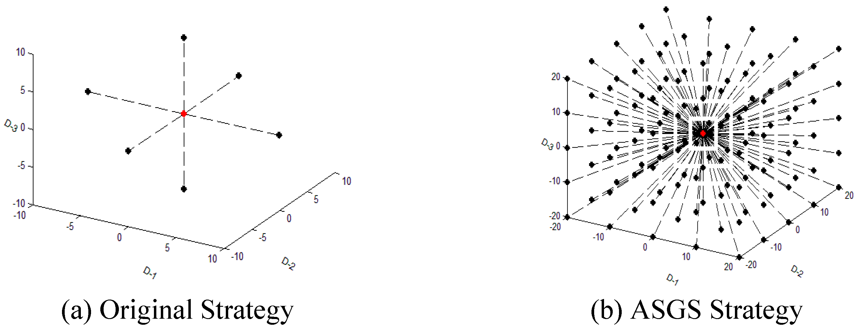
Figure 2.
Flow Chart of Original K-means Clustering.
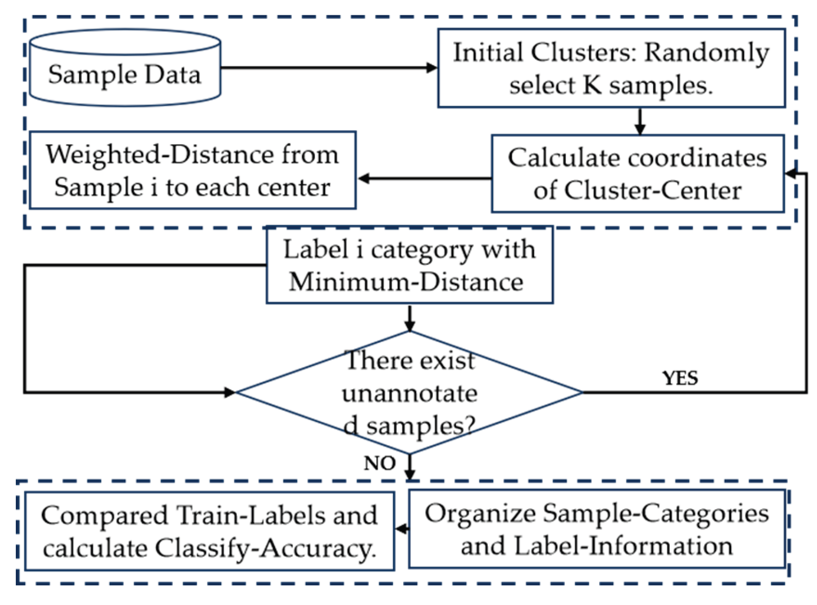
Figure 3.
Wolf Pack Algorithm Flow using Leadership Strategy.
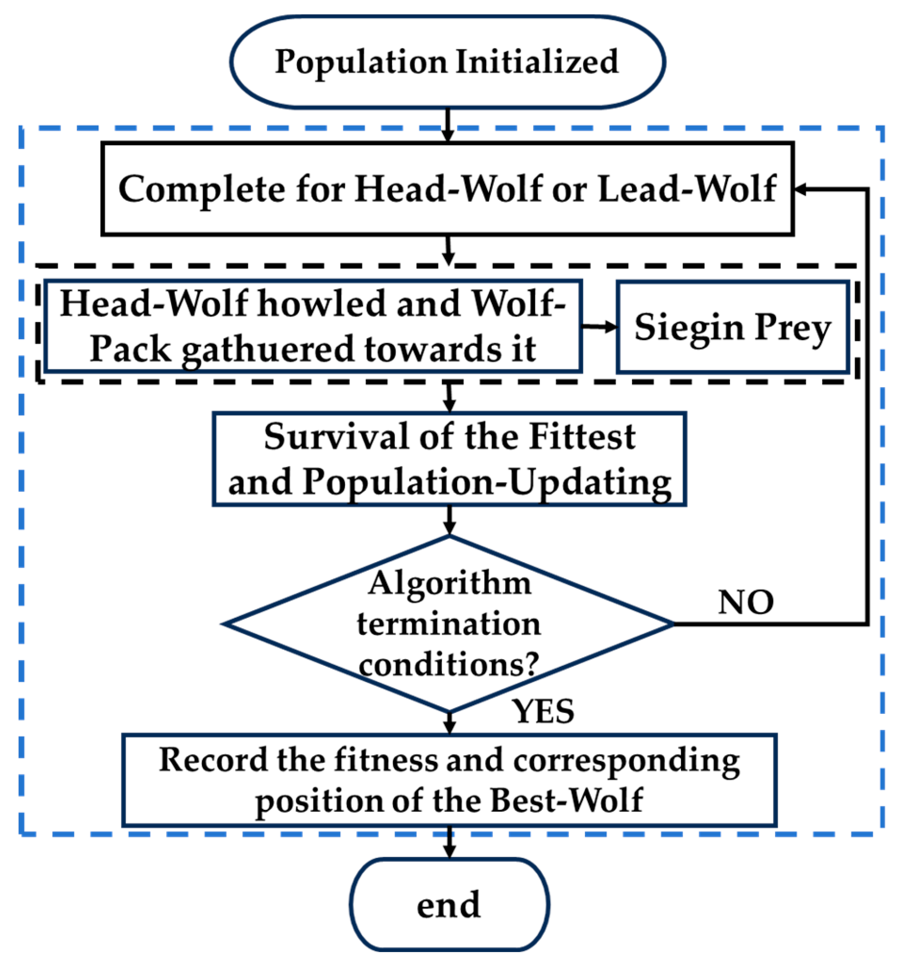
Figure 4.
Flow Chart of Original K-means Clustering optimized by AF-WPOA.
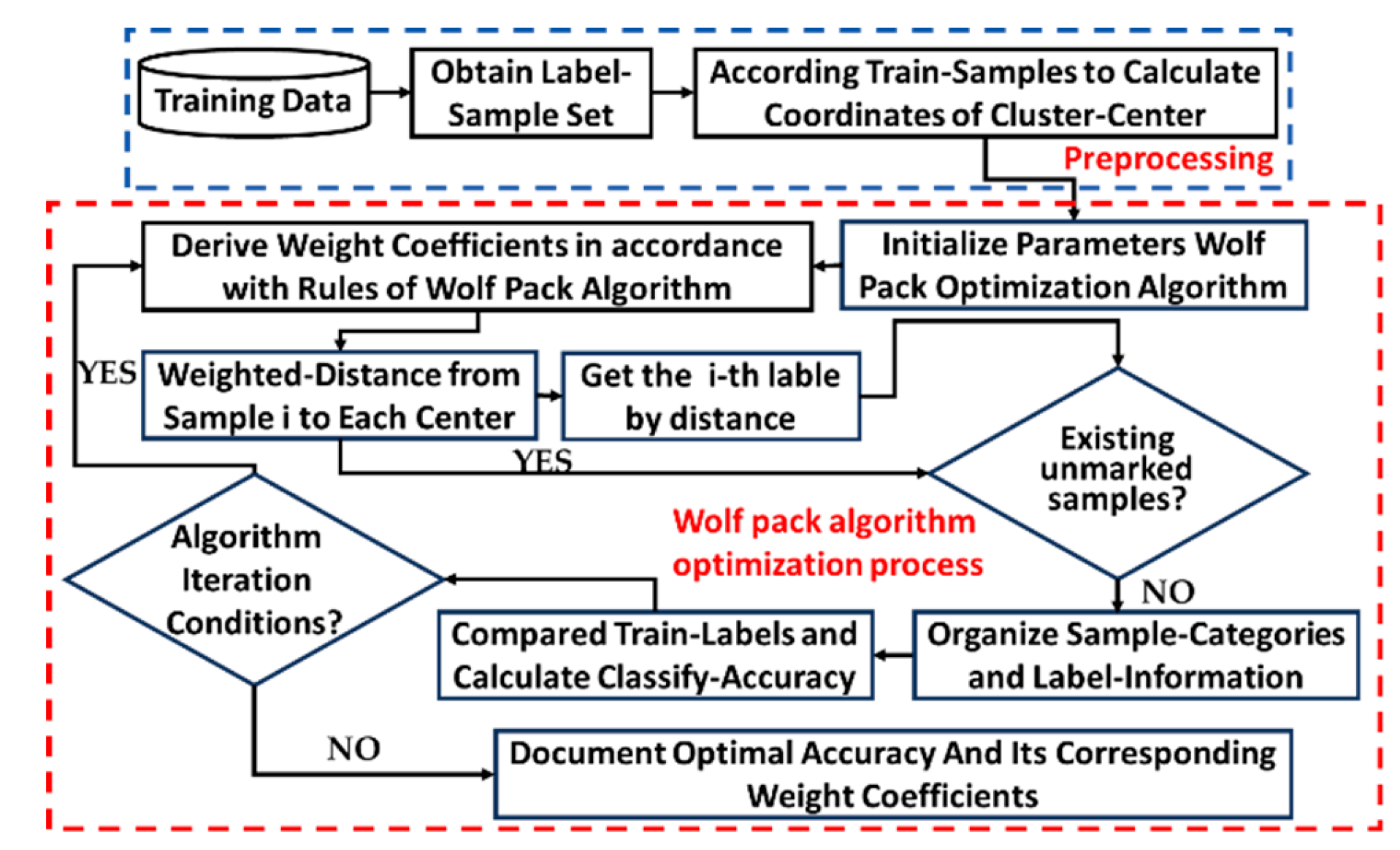
Figure 5.
Performance Comparison of Four Methods on Each Test Function.
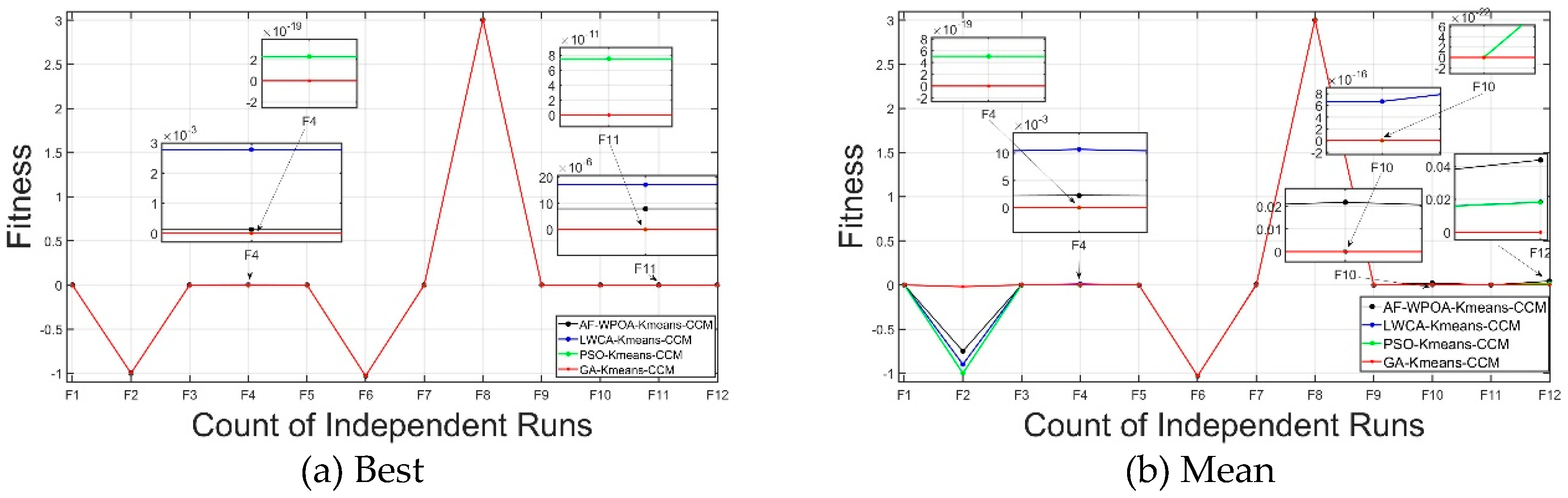
Figure 6.
Statistical Analysis Charts.
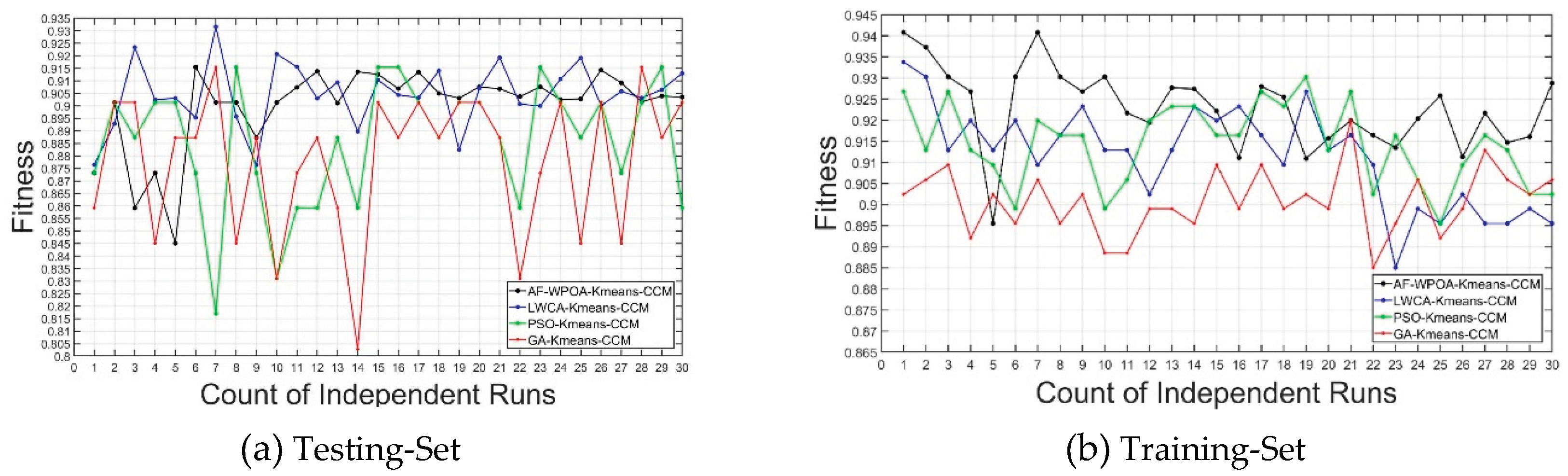

Table 1.
Algorithm Parameter Configuration.
| Order | Name | Configuration |
|---|---|---|
| 1 | GA [25] | Set the crossover probability to 0.7, the mutation probability to 0.01, and the generation gap to 0.95. |
| 2 | PSO | Individual acceleration value: 2, initial time weighting value: 0.9, convergence time weighting value: 0.4, restrict individual speed to 20% of the change range. |
| 3 | LWCA | Hunting stride length stepa: 0.75, summoning - charge stride length stepb: 0.45, siege threshold r0: 0.2, upper limit of siege stride length stepcmax=1e6, lower limit of siege stride length stepcmin=1e-2, update amount of wolf pack m: 5, maximum number of iterations T: 100, number of wolf groups: 50. |
| 4 | AF-WPOA | Hunting stride stepa: 0.75, summoning - rush stride stepb: 0.45, siege stride upper limit stepcmax = 1e6, siege stride lower limit stepcmin = 1e-2, maximum number of iterations T: 100; number of wolf pack populations: 50. |
Table 2.
Test Functions.
| Order | Function | Expression | Dimension | Range | Optimum |
| F1 | Matyas | F1 = 0.26×(x12 + x22) − 0.48×x1×x2 | 2 | [-10,10] | min f = 0 |
| F2 | Easom | F2 = − cos(x1)×cos(x2)× exp[−(x1 − π)2 − (x2 − π)2] | 2 | [-100,100] | min f = -1 |
| F3 | Sumsquares | F3 = 
|
10 | [-1.5,1.5] | min f = 0 |
| F4 | Sphere | F4= 
|
30 | [-1.5,1.5] | min f = 0 |
| F5 | Eggcrate | F5= x12 + x22+25×(sin2x1+ sin2 x2) | 2 | [-π,π] | min f = 0 |
| F6 | Six Hump Camel Back | F6 = 4×x1 - 2.1x14 + (1/3)×x16+x1×x2 - 4×x22 + 4×x24 | 2 | [-5,5] | min f = -1.0316 |
| F7 | Bohachevsky3 | F7= x12 + 2×x22 - 0.3×cos(3πx1 + 4πx2) + 0.3 | 2 | [-100,100] | min f = 0 |
| F8 | Bridge | F8= - 0.7129 - 0.7129 |
2 | [-1.5,1.5] | max f = 3.0054 |
| F9 | Booth | F9=(x1 + 2×x2 - 7)2 + (2×x1 + x2 - 5)2 | 2 | [-10,10] | min f = 0 |
| F10 | Bohachevsky1 | F10= x12 + 2x22 - 0.3×cos(3πx1) - 0.4×cos(4πx2)+0.7 | 2 | [-100,100] | min f = 0 |
| F11 | Ackley | F11=-20×exp(-0.2× ) -exp( ) -exp( ) +20 + e ) +20 + e |
6 | [-1.5,1.5] | min f = 0 |
| F12 | Griewank | 2 | [50,150] | min f = 0 |
Table 3.
Experimental Data.
| Function | GA | PSO | LWCA | AF-WPOA | ||||
|---|---|---|---|---|---|---|---|---|
| Best | Mean | Best | Mean | Best | Mean | Best | Mean | |
| F1 | 2.27E-13 | 2.13E-8 | 1.69E-31 | 1.06E-18 | 2.07E-24 | 3.35E-21 | 0 | 0 |
| F2 | -1 | -0.75001 | -1 | -0.90001 | -1 | -1 | -1 | -0.02 |
| F3 | 1.246E-8 | 1.92E-6 | 2.23E-6 | 3.6E-5 | 6.56E-19 | 2.44E-18 | 0 | 0 |
| F4 | 1.18E-4 | 2.26E-3 | 2.78E-3 | 1.07E-2 | 2.30E-19 | 5.05E-19 | 0 | 0 |
| F5 | 1.13E-11 | 4.13E-09 | 6.23E-24 | 1.42E-10 | 6.69E-22 | 6.55E-20 | 0 | 0 |
| F6 | -1.0316 | -1.0316 | -1.0316 | -1.0316 | -1.0316 | -1.0316 | -1.0316 | -1.0316 |
| F7 | 7.65E-12 | 6.79E-3 | 0 | 2.07E-14 | 0 | 0 | 0 | 0 |
| F8 | 3.0054 | 3.0038 | 3.0054 | 3.0054 | 3.0054 | 3.0054 | 3.0054 | 3.0054 |
| F9 | 4.93E-12 | 8.73E-10 | 5.62E-23 | 5.13E-18 | 7.33E-22 | 1.07E-19 | 0 | 0 |
| F10 | 8.43E-13 | 2.18E-2 | 0 | 6.67E-16 | 0 | 0 | 0 | 0 |
| F11 | 7.92E-06 | 5.17E-5 | 1.71E-5 | 1.14E-4 | 7.53E-11 | 2.44E-10 | 0 | 0 |
| F12 | 6.54E-12 | 4.38E-2 | 4.48e-06 | 1.83E-2 | 2.53e-10 | 1.82E-2 | 0 | 0 |
Table 4.
Feature vector of the sample set.
| Order | Contract | Correlation | Homogeneity | Energy | Encircle-City Feature | Encircle-City Feature Auxiliary |
|---|---|---|---|---|---|---|
| 1 | 6.08 | 0.82 | 0.66 | 0.14 | 0.38 | 0.49 |
| 2 | 5.4 | 0.8 | 0.63 | 0.09 | 0.36 | 0.43 |
| 3 | 2.94 | 0.88 | 0.75 | 0.22 | 0.37 | 0.42 |
| 4 | 7.92 | 0.73 | 0.59 | 0.08 | 0.34 | 0.41 |
| 5 | 8.09 | 0.77 | 0.64 | 0.13 | 0.34 | 0.51 |
| 6 | 7.81 | 0.79 | 0.65 | 0.14 | 0.33 | 0.46 |
| … … | ||||||
| 353 | 3.52 | 0.89 | 0.73 | 0.13 | 0.3 | 0.34 |
| 354 | 2.54 | 0.92 | 0.78 | 0.13 | 0.28 | 0.28 |
| 355 | 3.13 | 0.9 | 0.73 | 0.09 | 0.34 | 0.32 |
| 356 | 3.21 | 0.91 | 0.73 | 0.09 | 0.31 | 0.36 |
| 357 | 2.81 | 0.91 | 0.73 | 0.11 | 0.29 | 0.28 |
| 358 | 3.97 | 0.87 | 0.73 | 0.17 | 0.31 | 0.38 |
Table 5.
Results of Experiments.
| Order | Recognition Accuracy on Training-Set | Recognition Accuracy on Testing-Set | ||||||
| AF-WPOA-Kmeans-CCM | LWCA-Kmeans-CCM | PSO-Kmeans-CCM | GA-Kmeans-CCM | AF-WPOA-Kmeans-CCM | LWCA-Kmeans-CCM | PSO-Kmeans-CCM | GA-Kmeans-CCM | |
| 1 | 0.9408 | 0.9338 | 0.9268 | 0.9024 | 0.8732 | 0.8765 | 0.8732 | 0.8592 |
| 2 | 0.9373 | 0.9303 | 0.9129 | 0.9059 | 0.9014 | 0.8929 | 0.9014 | 0.9014 |
| 3 | 0.9303 | 0.9129 | 0.9268 | 0.9094 | 0.8592 | 0.9234 | 0.8873 | 0.9014 |
| 4 | 0.9268 | 0.9199 | 0.9129 | 0.892 | 0.8732 | 0.9024 | 0.9014 | 0.8451 |
| 5 | 0.8955 | 0.9129 | 0.9094 | 0.9024 | 0.8451 | 0.9031 | 0.9014 | 0.8873 |
| 6 | 0.9303 | 0.9199 | 0.899 | 0.8955 | 0.9155 | 0.8953 | 0.8732 | 0.8873 |
| 7 | 0.9408 | 0.9094 | 0.9199 | 0.9059 | 0.9014 | 0.9316 | 0.8169 | 0.9155 |
| 8 | 0.9303 | 0.9164 | 0.9164 | 0.8955 | 0.9014 | 0.8957 | 0.9155 | 0.8451 |
| 9 | 0.9268 | 0.9233 | 0.9164 | 0.9024 | 0.8873 | 0.8764 | 0.8732 | 0.8873 |
| 10 | 0.9303 | 0.9129 | 0.899 | 0.8885 | 0.9014 | 0.9207 | 0.831 | 0.831 |
| 11 | 0.9217 | 0.9129 | 0.9059 | 0.8885 | 0.9074 | 0.9156 | 0.8592 | 0.8732 |
| 12 | 0.9194 | 0.9024 | 0.9199 | 0.899 | 0.9138 | 0.903 | 0.8592 | 0.8873 |
| 13 | 0.9277 | 0.9129 | 0.9233 | 0.899 | 0.9011 | 0.9094 | 0.8873 | 0.8592 |
| 14 | 0.9274 | 0.9233 | 0.9233 | 0.8955 | 0.9136 | 0.8898 | 0.8592 | 0.8028 |
| 15 | 0.9222 | 0.9199 | 0.9164 | 0.9094 | 0.9126 | 0.9103 | 0.9155 | 0.9014 |
| 16 | 0.9111 | 0.9233 | 0.9164 | 0.899 | 0.9069 | 0.9044 | 0.9155 | 0.8873 |
| 17 | 0.928 | 0.9164 | 0.9268 | 0.9094 | 0.9135 | 0.9033 | 0.9014 | 0.9014 |
| 18 | 0.9255 | 0.9094 | 0.9233 | 0.899 | 0.905 | 0.914 | 0.8873 | 0.8873 |
| 19 | 0.9109 | 0.9268 | 0.9303 | 0.9024 | 0.9031 | 0.8825 | 0.9014 | 0.9014 |
| 20 | 0.9157 | 0.9129 | 0.9129 | 0.899 | 0.9076 | 0.9069 | 0.9014 | 0.9014 |
| 21 | 0.9199 | 0.9164 | 0.9268 | 0.9199 | 0.9068 | 0.9193 | 0.8873 | 0.8873 |
| 22 | 0.9164 | 0.9094 | 0.9024 | 0.885 | 0.9037 | 0.9007 | 0.8592 | 0.831 |
| 23 | 0.9135 | 0.885 | 0.9164 | 0.8955 | 0.9076 | 0.9 | 0.9155 | 0.8732 |
| 24 | 0.9204 | 0.899 | 0.9059 | 0.9059 | 0.9025 | 0.9107 | 0.9014 | 0.9014 |
| 25 | 0.9258 | 0.8955 | 0.8955 | 0.892 | 0.9028 | 0.9191 | 0.8873 | 0.8451 |
| 26 | 0.9113 | 0.9024 | 0.9094 | 0.899 | 0.9143 | 0.9001 | 0.9014 | 0.9014 |
| 27 | 0.9217 | 0.8955 | 0.9164 | 0.9129 | 0.9092 | 0.9058 | 0.8732 | 0.8451 |
| 28 | 0.9147 | 0.8955 | 0.9129 | 0.9059 | 0.9016 | 0.9032 | 0.9014 | 0.9155 |
| 29 | 0.9161 | 0.899 | 0.9024 | 0.9024 | 0.9039 | 0.9065 | 0.9155 | 0.8873 |
| 30 | 0.9288 | 0.8955 | 0.9024 | 0.9059 | 0.9035 | 0.913 | 0.8592 | 0.9014 |
Table 6.
Statistical Analysis of Experiments.
| Algorithm name | Accuracy | Notes | |
| Training-Set | Testing-Set | ||
| AF-WPOA-Kmeans-CCM | 93.03% | 91.55% | For 30 independent experiments, the sum of the classification accuracy on Training-Set and the one on Testing-Set is maximized, which indicates the overall optimal performance. |
| Kmeans-CCM | 81.88% | 87.32% | |
| GA-Kmeans-CCM | 90.59% | 91.55% | |
| PSO-Kmeans-CCM | 91.64% | 91.55% | |
| LWCA-Kmeans-CCM | 94.08% | 87.05% | |
Disclaimer/Publisher’s Note: The statements, opinions and data contained in all publications are solely those of the individual author(s) and contributor(s) and not of MDPI and/or the editor(s). MDPI and/or the editor(s) disclaim responsibility for any injury to people or property resulting from any ideas, methods, instructions or products referred to in the content. |
© 2025 by the authors. Licensee MDPI, Basel, Switzerland. This article is an open access article distributed under the terms and conditions of the Creative Commons Attribution (CC BY) license (http://creativecommons.org/licenses/by/4.0/).
Copyright: This open access article is published under a Creative Commons CC BY 4.0 license, which permit the free download, distribution, and reuse, provided that the author and preprint are cited in any reuse.


