
Submitted:
27 October 2025
Posted:
28 October 2025
You are already at the latest version
Abstract
The FWD is commonly used to conduct a non-destructive evaluation of the capacity of the pavement. The layered pavement is loaded locally by falling weight, and deflection at many points is recorded. Based on these results, knowing the pavement geometry, the mechanical properties of the pavement may be determined using the back-calculation approach. Some methods are used for back calculation, such as analytical, numerical, or ML. An analytical solution for a multi-layered structure leads to non-linear relationships for the thickness or stiffness of each layer, but gives an accurate solution. The other methods, like numerical or ML methods, are just approximation methods with different levels of accuracy. In this paper, the robustness of the XGBoost ML regression model in predicting mechanical and geometrical pavement parameters was estimated. The database was generated from a static analytical solution of an axially symmetrical problem implemented in the form of JPAV software and then explored by training regression models to predict moduli and thickness of pavement layers. Two other databases were created using PCA (Principal Component Analysis) and FDM (Feature Difference Method) to compare models trained with the complete deflection database. The results showed that models trained with the complete deflection database had the best average prediction performance compared to the other two. In contrast, models trained with the database pre-processed by PCA showed predicting performance similar to the previous models, but with a little precision loss. Models trained with the database pre-processed by FDM exhibited excellent prediction on some features but worse on the rest.
Keywords:
FWD
; XGBoost
; regression models
; prediction
; PCA
; FDM
; ML
1. Introduction
The average highway mileage of the top 3 countries with the largest total highway mileage has already reached 6 million kilometres by 2024 [1]. With the continuously increasing highway mileage, maintenance could play a more and more critical role than ever, and some countries, e.g. the US and Denmark, have already allocated a significant part of the road-related budget to it [2].
Considering the maintenance of pavement, the evaluation of pavement condition is a critical component of infrastructure management, necessitating robust assessment techniques. Two primary methodologies are utilized: destructive testing, such as coring, and non-destructive testing (NDT), exemplified by the Falling Weight Deflectometer (FWD). Coring involves the extraction of cylindrical pavement samples to directly characterize material properties, including compressive strength and asphalt content, as well as structural attributes, such as layer thickness and interlayer bonding. Despite its precision, this method causes permanent structural damage, requiring subsequent repairs that elevate costs and disrupt traffic flow. Conversely, NDT assesses pavement condition without compromising structural integrity, offering greater efficiency and the ability to cover larger areas compared to destructive methods. The FWD, a widely adopted NDT technique, generates a dynamic load pulse by dropping a calibrated weight onto a 300 mm diameter circular load plate, inducing vertical deformations that form a deflection basin (Figure 1) [3]. These deformations are measured using geophones positioned at the load center and at multiple radial distances, enabling rapid data acquisition over extensive pavement sections. The collected deflection data facilitate the prediction of pavement layer moduli and thicknesses through back-calculation techniques [4].
Back-calculation employs an iterative numerical optimization process to determine pavement properties. This process begins with an initial estimate of pavement properties, followed by a forward calculation to simulate the FWD test and compute the predicted deflection response. The computed response is then compared to the actual FWD deflection data, yielding a value for an objective function that quantifies the agreement between estimated properties and observed measurements. Through an optimization procedure, the estimated properties are iteratively adjusted to minimize the objective function, refining the accuracy of the pavement property predictions [5]. Compared to coring, which is labor-intensive and limited to discrete locations, the FWD enables efficient, large-scale assessments with minimal disruption. While coring provides precise, localized material data for detailed forensic analysis, NDT methods like the FWD preserve pavement integrity, making them ideal for routine monitoring and broad structural evaluations. The selection of an appropriate method depends on project objectives, balancing the need for detailed material characterization against the advantages of rapid, non-invasive assessment for effective pavement management.
Various programs are available to analyse the pavement structures, e.g. ELSYM5, WESLEA, BISAR, etc., or back-calculation tools like ELMOD. In static analysis, the peak load and deflection are used to calculate thickness and moduli of pavement layers. In contrast, in dynamic analysis e.g. DBALM, FEM, 3D-Move etc [6,7,8], the force-time recorded functions are directly utilised to predict needed results. However, based on research by Tarefder [9], the results from many back-calculation software vary, and the final output differs from the laboratory result due to the calculation algorithm.
Unlike traditional back-calculation analytical algorithms, ML is a popular tool for analysing similar tasks [10,11,12]. ANN is one of the most popular analysis tools that allows for reasonable predictions without referencing physical phenomena in analysed problems [13,14,15]. Pure ANN and hybrid models, e.g. combined with Genetic Algorithm, were utilized to predict the moduli of pavement. The results showed that ANN models improved prediction compared to traditional back-calculation software, and the hybrid ANN model showed stronger generalisation ability than traditional ANN [16,17,18].
Ensemble models are also popular ML models , e.g., RF (Random Forest) and GBM (Gradient Boosting Machines), which are commonly used to predict pavement properties. Sudyka et al.[19] used both RF, ANN and BT (Bagged Trees) Reinforced Trees to train different models to predict asphalt layer temperature based on data obtained from FWD and TSD. The results showed that all of the models had a nice prediction accuracy with R2 values of over 0.8. Worthey et al.[20] predicted the dynamic modulus of asphalt mixtures by a model trained in Bagged trees ensemble, and ensemble models exhibited a significantly better prediction accuracy on this property than some ANN models.
One of the ensemble models, XGBoost, performs better than other tree boosting models in practice [21]. With such an advantage, there is still little literature on back-calculation in specific FWD applications, while much other literature is analysing pavements and proving their performance. Wang et al. [22] found its performance of predicting the international roughness index of rigid pavement surpassed other ensemble models. In addition, Ali et al. [23] used XGBoost to predict the dynamic modulus of asphalt concrete mixtures, and the results exhibited significantly outperforming some of the well-known regression models, such as Witczak, Hirsch, and Al-Khateeb. Ahmed [24] built both RF and XGBoost models to predict pavement structural conditions based on data derived from the Long-Term Pavement Performance(LTPP) program. Results demonstrated that XGBoost outperformed RF and had practical advantages over empirical equations. Summarising, XGBoost presents better performance than other tree boosting models; in some cases, it outperforms ANN. However, there is little research on FWD back-calculation using XGBoost.
2. Objective and Methodology
The paper involved generating a deflection database using “JPAV (version 3.3)” software, simulating an axisymmetric problem of a layered half-space under load. Randomly generated layer properties yielded more than 60000 datasets. The pavement structures (elements of the generated database) were assessed with respect to their compliance (the inverse of stiffness). Compliance estimates were made using solutions to linear elasticity problems, assuming either uniform loading (which leads to a one-dimensional problem) or its localization (which leads to the interpretation of compliance within the framework of Kirchhoff's thin plate theory). Then, based on the database obtained and evaluated in this way, a machine learning model was built to predict the stiffness and thickness moduli of individual pavement layers. The study utilized an XGBoost regression model, trained after data pre-processing including splitting, standard scaling, and Optuna-based hyperparameter tuning. Model performance was assessed via R2 and RMSE. Two alternative pre-processing methods, PCA and FDM were also implemented and their results compared.
3. Database Generation
In order to generate a database, i.e., sets of input data (all parameters of the layered structure such as layer thicknesses and their material properties) and output data in the form of deflections at 10 distinguished points (as in the FWD test), a boundary value problem was formulated as in Figure 1. This is an axisymmetric problem of an infinite layered half-space symmetrically loaded on a circular area of radius a with a load equal to 40kN to consider the 80kN standard axle load.
A database for training the machine learning model was generated using “JPav” program developed by one of the authors, which was a static analytical deflection-calculation software that could calculate the deflection at a given point based on pavement layers’ properties. Pavement layers’ properties indicate thickness (Has) and modulus (Eas) of the asphalt layer, thickness (Hgr) and modulus (Hgr) of the granular layer, thickness (Hsu) and modulus (Esu) of the subgrade layer and modulus (Eil) of the infinite subgrade layer. While the results of defection at ten measuring points, d1 to d10, are the output of the software, the distance of the measuring points from the load center are 0, 0.2m, 0.3m, 0.45m, 0.6m, 0.9m, 1.2m, 1.5m, 1.8m, 2.1m, respectively.
To get the result from JPav, it requires at least 11 input parameters. The 4 constant inputs are the number of loads, magnitude of load (kN), the radius of contact circular area (m), and Poisson’s ratio of each layer, set as 1, 40, 0.15, 0.35, respectively. To get a continuous database for later analysis, the rest of the inputs, i.e. the properties of each layer, were generated randomly in a specific range, as shown in Table 1. In total, 65825 data sets have been randomly generated, consisting of the input data (geometrical and mechanical parameters of the structure) and output data (deflection values for points d1-d10).
4. Analysis of the Generated Database
Considering a continuous and even distribution of thickness and Young’s modulus of each layer within its range above, the database was generated using JPav. The distribution of the database input parameters is presented in Figure 2.
It should be noted that the randomly given geometric parameters (i.e. layer thicknesses) as well as mechanical parameters (layer stiffness moduli) generally define the pavement structure with a specific global stiffness (compliance). To evaluate the generated database, the compliance of individual pavement layers and the total compliance of layers (without taking into account the native soil layer of infinite thickness) were assessed. The compliance was assessed assuming a uniaxial stress state (compression) in the layer of isotropic elastic material, following the formulas resulting from the theory of elasticity [25,26]
where i=as, gr, su, il and h is the thickness of one layer, E is Young’s modulus of one layer and is Poisson’s ratio, herein, = 0.35. The summary compliance can be calculated as the following sum:
Assuming that at some depth H=15m-has-hgr-hsu there is a rigid layer top surface, then total compliance may be determined based on a displacement boundary condition. In this type of compliance estimation, the local nature of the load in the FWD test is not taken into account. Therefore, an estimation of the (bending) compliance based on Kirchhoff's thin plate theory was also proposed [27] determining the compliance of each layer according to the formula
Summary compliance (SBC) may be determined analogically like in case of axial compliance, see Eq. 2 and assumptions given below this equation. The real compliance of FWD problem is located somewhere between SC and SCB.
Following the equations above for the analysed database, the distributions in terms of compliances are shown in Figure 3. It can be seen that in all cases in the data set, an increased number of layers with lower compliance (higher stiffness).
The compliance of individual layers contributes to the overall compliance of the pavement structure. Figure 4 presents histograms of the total compliances, SBC and SC. These histograms do not conform to normal distributions but resemble gamma distributions. However, statistical analysis does not support this conclusion at a 95% confidence level. Comparing the distributions of total compliance with those of individual layers reveals a shift in their characteristics. The database predominantly contains cases with medium compliance, with fewer cases exhibiting low compliance. Cases with high compliance are also significant in number.
This section above presents the analysis of input data for the ML algorithm. The data were processed using JPav to generate the output dataset, comprising ten deflection points (d1-d10) that define the deflection basin. The output data underwent statistical evaluation, with results presented in Table 2. In addition, multicollinearity assessment is essential for high-dimensional datasets. Elevated multicollinearity within a dataset complicates the isolation of individual effects of correlated features on the target variable, potentially compromising the interpretability and reliability of predictive models [28]. So, a Pearson correlation matrix was computed, with results visualised as a heatmap in Figure 5. To facilitate analysis across varying distances, each distance (r) was normalized by the radius of the loading plate (a), as described below:
where is the normalized distance, a is the radius of loading, (herein a = 0.15m) and r is the radial distance of the measuring point from the axis of symmetry, in m.
Analysis of the correlation matrix heatmap (Figure 5) reveals a strong correlation between neighbouring measurement points within the range d1 to d5. Beyond this range, deflections correlate strongly not only with adjacent points but also with two or three subsequent points. Consequently, reducing the number of measurement points in the range d6 to d10 (for ) is unlikely to significantly affect the accuracy of data used for back-analysis in interpreting FWD test results.
Table 2 summarises the average, maximum, and minimum deflection values, which characterise a typical deflection basin. All skewness values are positive, indicating a right-skewed distribution. Kurtosis values are less than 3 (the kurtosis of a normal distribution), indicating a platykurtic distribution with fewer outliers. This is confirmed by the absence of outliers within the homogeneous interval [Q1-1.5IRQ; Q3 + 1.5IRQ]. Approximately 3% of the data were identified as outliers and will be removed from the dataset prior to training the machine learning model. After removing these outliers, the dataset contains 60687 data points.
5. ML Model: Its Algorithm and Training
5.1. The Algorithm
XGBoost is used for prediction, which stands for eXtrem Gradient Boosting, an instance of GBM (Gradient Boosting Machine). And it is a modification of Greedy Forest that introduces regularisation, employs a second-order expansion of the loss function, and implements a novel, more efficient greedy-search strategy. This algorithm within it is a type of ensemble learning method, which predicts outputs (i.e. ) by combining multiple weak trees. Results can be predicted from the variables and t additive functions [29,30] as
where is an independent tree structure specified by leaf score, and is the space of regression trees. XGBoost gets outputs by creating a new tree , which fits the residual error between the value from the previous tree and the actual value [24]. Function is a split function that assigns each input to one of its leaf indices and is a set of leaf weights.
The process can be presented as:
where is the predicted value at the t-1-th tree, is the residual fitting value from the new built tree with input . To get more precise predictions, the following object function is minimized:
where is the loss function, defined as the squared error in regression trees: and stands for given data. is the regularization term on the number of leaves. t represents the number of leaves in the newly added tree at the t-th round, and is hyperparameter to control the complexity of the tree. is the L2 regularization term on the leaf weights. controls the magnitude of the leaf weights, represents the weight associated with the j-th leaf in the newly added tree. Weights for leaves are optimised with , which is second-order expansion of the loss function dropped the term which does not depend on . After calculations optimised weights are:
where and are the sum of the first and the second derivative of calculated at for a fixed tree. The value of modified object function without for equals to:
Minimisation proceeds node-by-node: for every candidate split the algorithm computes the loss-reduction term (gain) and greedily chooses the split with the largest positive value.
5.2. Models Training
Before training XGBoost models, there two steps normally, the first step is data pre-precessing and the second is hyperparameters tuning.
5.2.1. Data Pre-Processing
- The dataset was imported, and all observations with missing values were removed.
- The dataset was split into training and test sets in a 3:1 training-to-test ratio.
- Standard scaling was applied to the training dataset.
5.2.2. Tuning of Hyperparameters
Hyperparameters were tuned using 10-fold cross-validation with Optuna (version 4.2.0) [31]. The tuned hyperparameters fall into two categories: tree architecture and regularisation (see Error! Reference source not found.). Fixed hyperparameters, including the objective (reg:squarederror), early_stopping_rounds (10), and random_state (42), were set accordingly.

Table 3.
Hyperparameters after Optuna tuning.
| Category | Hyperparameters | Values | Role in the model |
| Architecture | n_estimators | 12000 | Number of boosted trees. Increasing this value can improve accuracy but also training time and the risk of overfitting. |
| learning_rate | 0.19 | Shrinkage factor applied to each tree’s contribution. Lower values require more trees but often generalise better. | |
| max_depth | 6 | Maximum depth of an individual tree. Shallower trees are less expressive but more robust. | |
| subsample | 0.93 | Fraction of training instances sampled for every tree, introducing bagging-style variance reduction. | |
| colsample_bytree | 0.95 | Fraction of predictor variables sampled for every tree, further decorrelating the ensemble. |
|
| Regularisation | Gamma (γ) | 0.03 | Minimum loss reduction required to split a node. Acts as a complexity penalty: higher γ prunes weak splits. |
| reg_alpha | 8.15 | L1 penalty on leaf weights | |
| reg_lambda (λ) | 1.41 | L2 penalty on leaf weights |
Optuna [32] frames hyperparameters tuning as a black-box optimisation loop built around a define-by-run API, so the search space is created dynamically inside the objective function rather than declared up-front. It begins with a Tree-structured Parzen Estimator (TPE) [33] to explore broadly, then—once trial data reveal correlations, can hand off to a relational sampler such as CMA-ES [34], which adapts a full covariance matrix to intensify search in the most promising region. Throughout, an asynchronous variant of Successive Halving (ASHA) [35] monitors intermediate validation scores and culls under-performing trials on the fly, recycling compute into better candidates. In short, the combination of dynamic search-space construction, hybrid Bayesian/evolutionary sampling, and aggressive early-pruning delivers fast, resource-efficient convergence to high-quality hyperparameters settings.
6. ML Models: Evaluation
6.1. Models Training with Whole Dataset
Based on the preparation in last Section, models were trained using XGBoost (version 2.1.4) [36]. Their performance was evaluated using the coefficient of determination (R2) and root mean square error (RMSE), with results presented in Table 4.
The results indicate that models predicting Has, Hsu, and Esu achieved strong performance, with coefficients of determination (R2) exceeding 0.8. However, models for Hgr and Eil exhibited poor performance, with R2 values below 0.1.
To interpret these models, feature importance (FI) and SHAP violin plots were employed, as detailed below. FI quantifies the influence of each input feature on the model’s predictions [37], as presented in Figure 6.
The analysis of the feature importance, as depicted in Figure 6, reveals that deflections at positions d1, d6, and d10 exert significant influence on the prediction of Has, Esu, and Hsu, respectively, with importance values exceeding 0.5. Notably, d10 also demonstrates a substantial impact on the prediction of Eil. For the prediction of Eas, deflections at d1 and d2 exhibit greater influence compared to other features, with importance values approximately 0.2. In contrast, the remaining features show negligible influence on predictive performance, with importance values below 0.2, and some approaching zero.
To elucidate the contribution of each feature to the model, SHAP (SHapley Additive exPlanations) violin plots were employed. These plots visualize the SHAP values, which quantify the contribution of each predictor to the model’s output. The violin plots illustrate the distribution of these contributions, highlighting the magnitude and direction (positive or negative) of each feature’s impact on predictions. The SHAP violin plots are presented in Figure 7.
Analysis of the SHAP violin plots reveals distinct dominant features for various target variables. Specifically, for the targets Has, Hgr, Hsu, Eas, Egr, Esu, and Eil, the corresponding dominant features are deflections at positions d1, d10, d10, d1 and d2, all positions, d6 and d10, and d10, respectively. Examination of Figure 6 and Figure 7, indicates that models exhibiting high predictive performance, such as those for Has, Hsu, and Eas, are characterised by a limited number of dominant features. For instance, in the violin plot for Has (Figure 6a), the deflection at d1 emerges as the dominant feature, demonstrating a consistent influence on predictions, as evidenced by its broader span along the x-axis compared to other features. Additionally, certain features exhibit minimal importance in predictive tasks, prompting consideration of feature reduction techniques, which are discussed in subsequent sections.
6.2. Model Training with PCA
Principal Component Analysis (PCA) is a widely utilised dimensionality reduction technique that identifies a reduced set of orthogonal features, or principal components, capable of representing the original dataset in a lower-dimensional subspace while minimising information loss [38]. The correlation analysis detailed in Section 3, coupled with the extensive dataset comprising 60687 samples, indicates a highly correlated and voluminous database, rendering it well-suited for PCA.
During the data pre-processing phase, the methodology closely followed the procedures outlined previously, with the sole distinction occurring post-data scaling. At this stage, PCA transformation was applied to the entire dataset. The explained variance ratio of each principal component is illustrated in Figure 8. To ensure that 99% of the variance is accounted for, three principal components (PC1, PC2, and PC3) were selected for model training. These components were subsequently utilized to train the predictive models. The results of the trained models are presented in Figure 9 and Figure 10.
Subsequently, XGBoost regression models were trained on the whole dataset using the same hyperparameters as those applied to the PCA-processed dataset. The performance of the models for each target property was evaluated using the coefficient of determination (R²) and root mean square error (RMSE). The results are presented in Table 5 (in case of the whole dataset), Figure 9 and Figure 10 (in case of reduced database with application of PCA approach).
Based on the results presented in Table 5 and the accompanying figures, the trained models for Has, Hsu, and Esu exhibit satisfactory predictive performance, achieving R² values exceeding 0.8. In contrast, the predictive performance of the remaining models is suboptimal. A comparison with the models trained in Subsection 6.1 reveals that the models exhibiting both high and poor predictive performance are consistent across datasets pre-processed with and without PCA. However, the predictive capabilities of the models for most properties show a slight decline, as indicated by reductions in R² and increases in RMSE, with the notable exception of the Has model, which maintains nearly equivalent predictive performance.
6.3. Model Training with FDM
The Feature Difference Method (FDM) generates a new database comprising deflection differences between adjacent points, as described in [39]. Drawing on prior studies [40,41], four variables were employed: sci, bdi, bci, and ci, in which sci and bdi were the differences between adjacent points in [40] These variables are detailed as follows:
The variables sci, bdi, bci, and ci represent the deflection differences between adjacent points, while d1, d3, d5, d6, d7, and d8 correspond to the deflections measured at the 1st, 3rd, 5th, 6th, 7th, and 8th points, respectively.
The model training process closely mirrored the methodology described previously, with the sole distinction being the substitution of the training database with the variables sci, bdi, bci, and ci during the data preprocessing stage. Following model training and prediction, the performance was assessed using the coefficient of determination (R²) and root mean square error (RMSE). The results are presented in Table 6 and visualised in Figure 11 and Figure 12.
Based on the results presented in Table 6 and the accompanying figures, the predictive performance of the models varies significantly across target properties. Only the model for Has (Figure 11a) achieves a satisfactory performance, with an R² value exceeding 0.8. The models for Eas (Figure 11d) and Esu (Figure 11f) approach this threshold, with R² values close to 0.8. However, the remaining models exhibit poor predictive performance. Notably, the models for Hgr (Figure 11b) and Eil (Figure 11g) yield R² values near zero, indicating an extremely poor fit to the dataset when compared to other trained models.
To facilitate a direct comparison of the predictive models trained using different preprocessing methods, the R² values are compiled and presented in Table 7.
In summary, a comparative analysis of the models trained in this study reveals that models utilizing full deflection data from 10 measuring points outperform both PCA-preprocessed and FDM-pre-processed models. Notably, the models for Hsu and Esu achieve R² values exceeding 0.9, indicating exceptional predictive capability. In contrast, models trained with PCA-pre-processed data exhibit moderate predictive performance, with nearly all models failing to surpass the predictive accuracy of those trained on full deflection data. However, these PCA-based models display a similar trend in predictive performance, excelling in predictions for Has, Hsu, and Esu, while performing poorly for other properties. Given that the PCA-pre-processed dataset is less than half the size of the full dataset, this approach significantly reduces computational resource demands, particularly for large databases.
Models trained with FDM-pre-processed data demonstrate superior performance in predicting Has, achieving an R² of approximately 0.919, which surpasses all other models, as well as notable performance for Eas. However, their predictive capabilities for the remaining properties are markedly inferior compared to both the whole dataset and PCA-pre-processed models.
7. Conclusions
This study developed a deflection database using the static analysis software JPav, which was subsequently utilized to train XGBoost regression models for back-calculating pavement properties. The key findings are summarized as follows:
- Correlation Analysis of Deflection Data: Analysis of the deflection database revealed significant correlations between adjacent measuring points. The strength of these correlations was inversely proportional to the distance between the points.
- Predictive Performance of XGBoost Models: XGBoost models trained on the deflection database demonstrated robust predictive performance for Has, Hsu, and Esu, achieving R² values exceeding 0.8. However, predictions for Hgr and Eil were notably poor, with R² values below 0.1.
- Feature Importance and SHAP Analysis: Feature importance (FI) analysis indicated that deflections at positions d1, d6, and d10 significantly influenced the predictions of Has, Esu, and Hsu, respectively. Furthermore, SHAP violin plots highlighted variations in dominant features across different target properties.
- Performance of PCA-Pre-processed Models: Models trained on data pre-processed using Principal Component Analysis (PCA) exhibited predictive capabilities comparable to those trained on the full deflection database, with Has, Hsu, and Esu models achieving R² values above 0.8. However, these models generally underperformed relative to those trained on the full dataset. Notably, PCA reduced the database dimensionality to four components, substantially lowering computational resource requirements.
- Performance of FDM-Preprocessed Models: Models trained on data preprocessed using the Feature Difference Method (FDM) excelled in predicting Has and Eas, outperforming all other models trained with different methods. However, predictive performance for the remaining properties was inferior compared to models trained on the whole dataset or PCA-preprocessed datasets.
- Despite the application of various preprocessing methods—full deflection database, PCA, and FDM-the prediction of the granular layer thickness (Hgr) and the modulus of the infinite layer (Eil) remained consistently poor. None of the models achieved satisfactory performance, with R² values failing to exceed 0.8 for these properties.
Author Contributions
Conceptualization, M.G., P.X., B.G. and J.P.; methodology, M.G., P.X., B.G and J.P.; formal analysis, M.G. and P.X.; data curation, M.G. and P.X.; writing—original draft preparation, M.G. and P.X.; writing—review and editing, M.G., P.X., B.G., J.P. and M. M; visualization, P.X. and B.G.; supervision, M.G. All authors have read and agreed to the published version of the manuscript.
Abbreviations
The following abbreviations are used in this manuscript:
| FWD | Falling Weight Deflectometer |
| XGBoost | eXtrem Gradient Boosting |
| ML | Machine Learning |
| PCA | Principal Components Analysis |
| FDM | First Difference Method |
| ANN | Artificial Neural Network |
| RF | Random Forests |
| GBM | Gradient Boosting Machine |
| LTPP | Long-Term Pavement Performance |
| RMSE | Root Mean Square Error |
| FI | Feature Importance |
| SHAP | SHapley Additive exPlanations |
References
- TOI World Desk World ’ s Largest Road Networks 2024 : The United States and India Take Top Spots (Updated: Oct 23, 2024, 11:20 IST). The Times of India 2024.
- Azarijafari, H.; Yahia, A.; Ben Amor, M. Life Cycle Assessment of Pavements: Reviewing Research Challenges and Opportunities. J. Clean. Prod. 2016, 112, 2187–2197. [Google Scholar] [CrossRef]
- Domitrović, J.; Rukavina, T. Application of GPR and FWD in Assessing Pavement Bearing Capacity. Rom. J. Transp. Infrastruct. 2013, 2, 11–21. [Google Scholar] [CrossRef]
- Rohde, G.T. Determining Pavement Structural Number from FWD Testing. Transp. Res. Rec. 1994, 61–68. [Google Scholar]
- Guzina, B.B.; Osburn, R.H. Feasibility of Backcalculation Procedures Based on Dynamic FWD Response Data. Transp. Res. Rec. 2005, 30–37. [Google Scholar] [CrossRef]
- Kanai, T.; Matsui, K.; Himeno, K. Applicability of Static and Dynamic Analytical Methods to Structural Evaluation of Flexible Pavements Using FWD Data. 7th Int. Conf. Bear. Capacit. Roads, Railw. Airfields, 2005. [Google Scholar]
- Hamim, A.; Yusoff, N.I.M.; Ceylan, H.; Rosyidi, S.A.P.; El-Shafie, A. Comparative Study on Using Static and Dynamic Finite Element Models to Develop FWD Measurement on Flexible Pavement Structures. Constr. Build. Mater. 2018, 176, 583–592. [Google Scholar] [CrossRef]
- Siddharthan, R.V.; Hajj, E.Y.; Sebaaly, P.E.; Nitharsan, R. Formulation and Application of 3D-Move: A Dynamic Pavement Analysis Program; Report: FHWA-RD-WRSC-UNR-201506; University of Nevada: Reno, NV, USA, 2015. [Google Scholar]
- Tarefder, R.A.; Ahmed, M.U. Consistency and Accuracy of Selected FWD Backcalculation Software for Computing Layer Modulus of Airport Pavements. Int. J. Geotech. Eng. 2013, 7, 21–35. [Google Scholar] [CrossRef]
- Miani, M.; Dunnhofer, M.; Rondinella, F.; Manthos, E.; Valentin, J.; Micheloni, C.; Baldo, N. Bituminous Mixtures Experimental Data Modeling Using a Hyperparameters-optimized Machine Learning Approach. Appl. Sci. 2021, 11. [Google Scholar] [CrossRef]
- Rondinella, F.; Daneluz, F.; Hofko, B.; Baldo, N. Improved Predictions of Asphalt Concretes’ Dynamic Modulus and Phase Angle Using Decision-Tree Based Categorical Boosting Model. Constr. Build. Mater. 2023, 400, 132709. [Google Scholar] [CrossRef]
- Baldo, N.; Daneluz, F.; Valentin, J.; Rondinella, F.; Vacková, P.; Gajewski, M.D.; Król, J.B. Mechanical Performance Prediction of Asphalt Mixtures: A Baseline Study of Linear and Non-Linear Regression Compared with Neural Network Modeling. Roads Bridg. - Drog. i Most. 2025, 24, 27–35. [Google Scholar] [CrossRef]
- Rondinella, F.; Oreto, C.; Abbondati, F.; Baldo, N. A Deep Neural Network Approach towards Performance Prediction of Bituminous Mixtures Produced Using Secondary Raw Materials. Coatings 2024, 14. [Google Scholar] [CrossRef]
- Baldo, N.; Manthos, E.; Pasetto, M. Analysis of the Mechanical Behaviour of Asphalt Concretes Using Artificial Neural Networks. Adv. Civ. Eng. 2018, 2018. [Google Scholar] [CrossRef]
- Pais, J.; Thives, L.; Pereira, P. Artificial Neural Network Models for the Wander Effect for Connected and Autonomous Vehicles to Minimize Pavement Damage. In Proceedings of the Proceedings of the 10th International Conference on Maintenance and Rehabilitation of Pavements; Pereira, P., Pais, J., Eds.; Springer Nature Switzerland: Cham, 2024; pp. 471–481. [Google Scholar]
- Tarawneh, B.; Munir, /; Nazzal, D. ; Nazzal, M.D. Optimization of Resilient Modulus Prediction from FWD Results Using Artificial Neural Network. Period. Polytech. Civ. Eng. 2014, 58, 143–154. [Google Scholar] [CrossRef]
- Li, M.; Wang, H. Development of ANN-GA Program for Backcalculation of Pavement Moduli under FWD Testing with Viscoelastic and Nonlinear Parameters. Int. J. Pavement Eng. 2019, 20, 490–498. [Google Scholar] [CrossRef]
- Han, C.; Ma, T.; Chen, S.; Fan, J. Application of a Hybrid Neural Network Structure for FWD Backcalculation Based on LTPP Database. Int. J. Pavement Eng. 2022, 23, 3099–3112. [Google Scholar] [CrossRef]
- Sudyka, J.; Mechowski, T.; Matysek, A. OPTIMISATION OF BELLS3 MODEL COEFFICIENTS TO INCREASE THE PRECISION OF ASPHALT LAYER TEMPERATURE CALCULATIONS IN FWD AND TSD MEASUREMENTS OPTYMALIZACJA WSPÓŁCZYNNIKÓW MODELU BELLS3 W CELU ZWIĘKSZENIA PRECYZJI OBLICZEŃ TEMPERATURY WARSTW. 2024, 23, 437–456. [CrossRef]
- Worthey, H.; Yang, J.J.; Kim, S.S. Tree-Based Ensemble Methods: Predicting Asphalt Mixture Dynamic Modulus for Flexible Pavement Design. KSCE J. Civ. Eng. 2021, 25, 4231–4239. [Google Scholar] [CrossRef]
- Nielsen, D. Tree Boosting With XGBoost Why Does XGBoost Win “Every” Machine Learning Competition?, Norwegian University of Science and Technology, 2016.
- Wang, C.; Xiao, W.; Liu, J. Developing an Improved Extreme Gradient Boosting Model for Predicting the International Roughness Index of Rigid Pavement. Constr. Build. Mater. 2023, 408, 133523. [Google Scholar] [CrossRef]
- Ali, Y.; Hussain, F.; Irfan, M.; Buller, A.S. An EXtreme Gradient Boosting Model for Predicting Dynamic Modulus of Asphalt Concrete Mixtures. Constr. Build. Mater. 2021, 295, 123642. [Google Scholar] [CrossRef]
- Ahmed, N.S. Machine Learning Models for Pavement Structural Condition Prediction : A Comparative Study of Random Forest ( RF ) and EXtreme Gradient Boosting ( XGBoost ). 2024, 570–586. [CrossRef]
- De Pascalis, R. The Semi-Inverse Method in Solid Mechanics: Theoretical Underpinnings and Novel Applications, A thesis submitted to the Universit´e Pierre et Marie Curie and Universit`a del Salento, 2010.
- Timoshenko, S.; Goodier, J.N. Theory of Elasticity. J. Elast. 1986, 49, 143–427. [Google Scholar]
- Timoshenko, S.; Woinowsky-Krieger, S. Theory of Plates and Shells. 1959.
- Chan, J.Y. Le; Leow, S.M.H.; Bea, K.T.; Cheng, W.K.; Phoong, S.W.; Hong, Z.W.; Chen, Y.L. Mitigating the Multicollinearity Problem and Its Machine Learning Approach: A Review. Math. 2022, Vol. 10, Page 1283 2022, 10, 1283. [Google Scholar] [CrossRef]
- Asselman, A.; Khaldi, M.; Aammou, S. Enhancing the Prediction of Student Performance Based on the Machine Learning XGBoost Algorithm. Interact. Learn. Environ. 2023, 31, 3360–3379. [Google Scholar] [CrossRef]
- Chen, T.; Guestrin, C. XGBoost: A Scalable Tree Boosting System. Proc. ACM SIGKDD Int. Conf. Knowl. Discov. Data Min. 2016, 13-17, 785–794. [Google Scholar] [CrossRef]
- Optuna: A Hyperparameter Optimization Framework — Optuna 4.3.0 Documentation.
- Akiba, T.; Sano, S.; Yanase, T.; Ohta, T.; Koyama, M. Optuna: A Next-Generation Hyperparameter Optimization Framework. 2019.
- Bergstra, J.; Bardenet, R.; Bengio, Y.; Kégl, B. Algorithms for Hyper-Parameter Optimization.
- Hansen, N.; Ostermeier, A. Completely Derandomized Self-Adaptation in Evolution Strategies. Evol. Comput. 2001, 9, 159–195. [Google Scholar] [CrossRef] [PubMed]
- Jamieson, K.; Talwalkar, A. Non-Stochastic Best Arm Identification and Hyperparameter Optimization. Proc. 19th Int. Conf. Artif. Intell. Stat. AISTATS 2016 2015, 240–248. [Google Scholar]
- XGBoost Documentation — Xgboost 3.0.2 Documentation.
- Hooker, S.; Erhan, D.; Kindermans, P.J.; Kim, B. A Benchmark for Interpretability Methods in Deep Neural Networks. Adv. Neural Inf. Process. Syst. 2019, 32. [Google Scholar]
- Kherif, F.; Latypova, A. Chapter 12 - Principal Component Analysis. In Machine Learning; Mechelli, A., Vieira, S., Eds.; Academic Press, 2020; pp. 209–225 ISBN 978-0-12-815739-8.
- Peterson, C.; Karl, R.; Jamason, P.F.; Easterling, D.R. First Difference Method : Maximizing Station Density for the Calculation of Long-Term Global Temperature Change. 1998, 103. 103.
- Talvik, O.; Aavik, A. USE OF FWD DEFLECTION BASIN PARAMETERS ( SCI, BDI, BCI ) FOR PAVEMENT CONDITION ASSESSMENT. 2009, 4, 196–202. [CrossRef]
- Chen, D.-H. Determination of Bedrock Depth from Falling Weight Deflectometer Data. Transp. Res. Rec. 1655 1999, 127–135. [Google Scholar] [CrossRef]
Figure 1.
Schematic diagram of the boundary value problem modelling the FWD test.
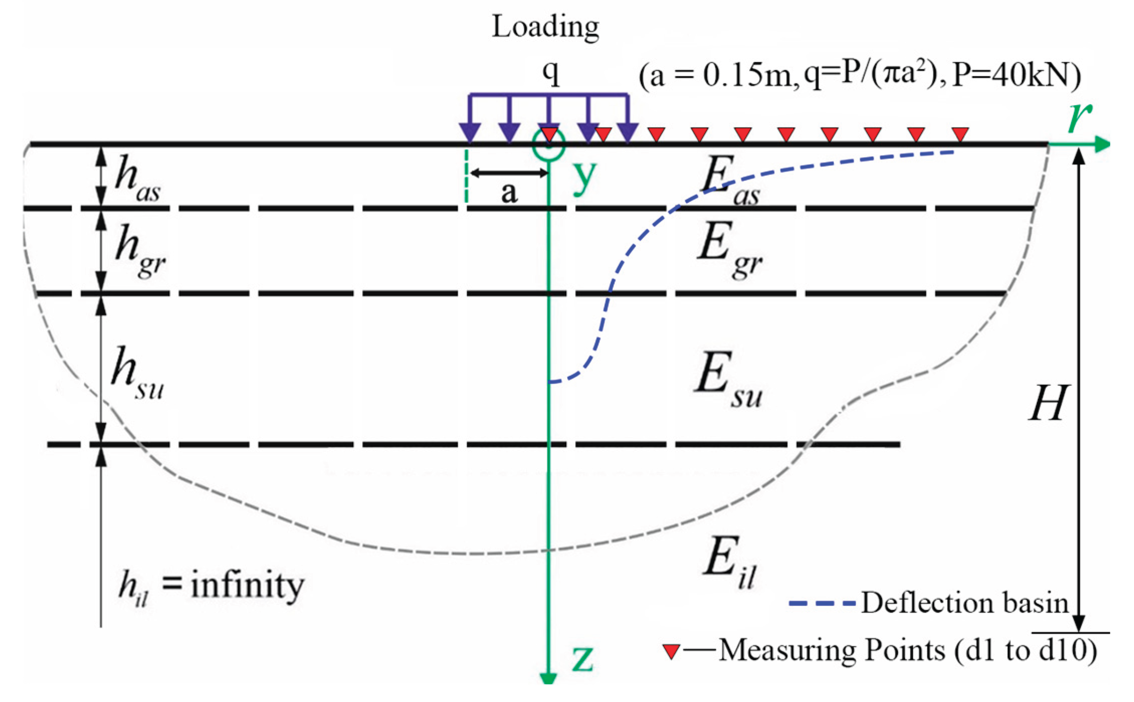
Figure 2.
Distribution of the database regarding the following input parameters.
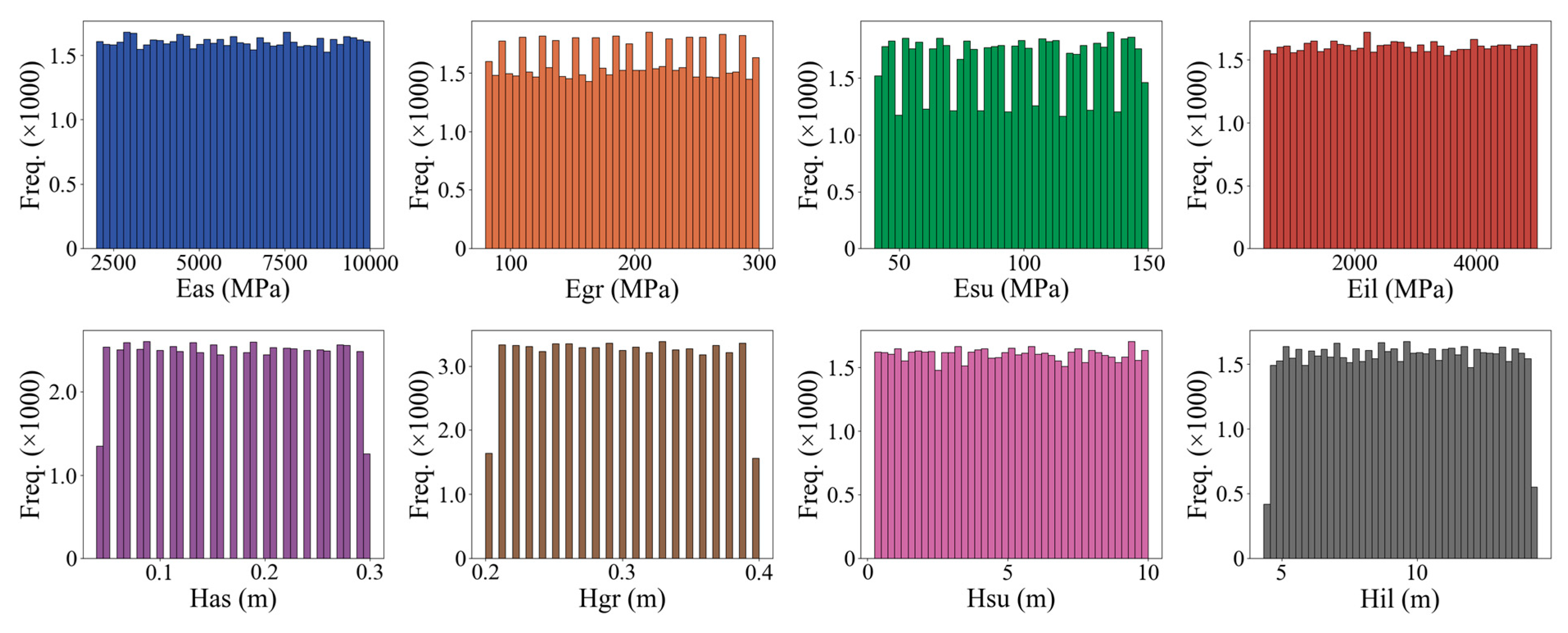
Figure 3.
Distribution of Ci and BCi for the following pavement layers.
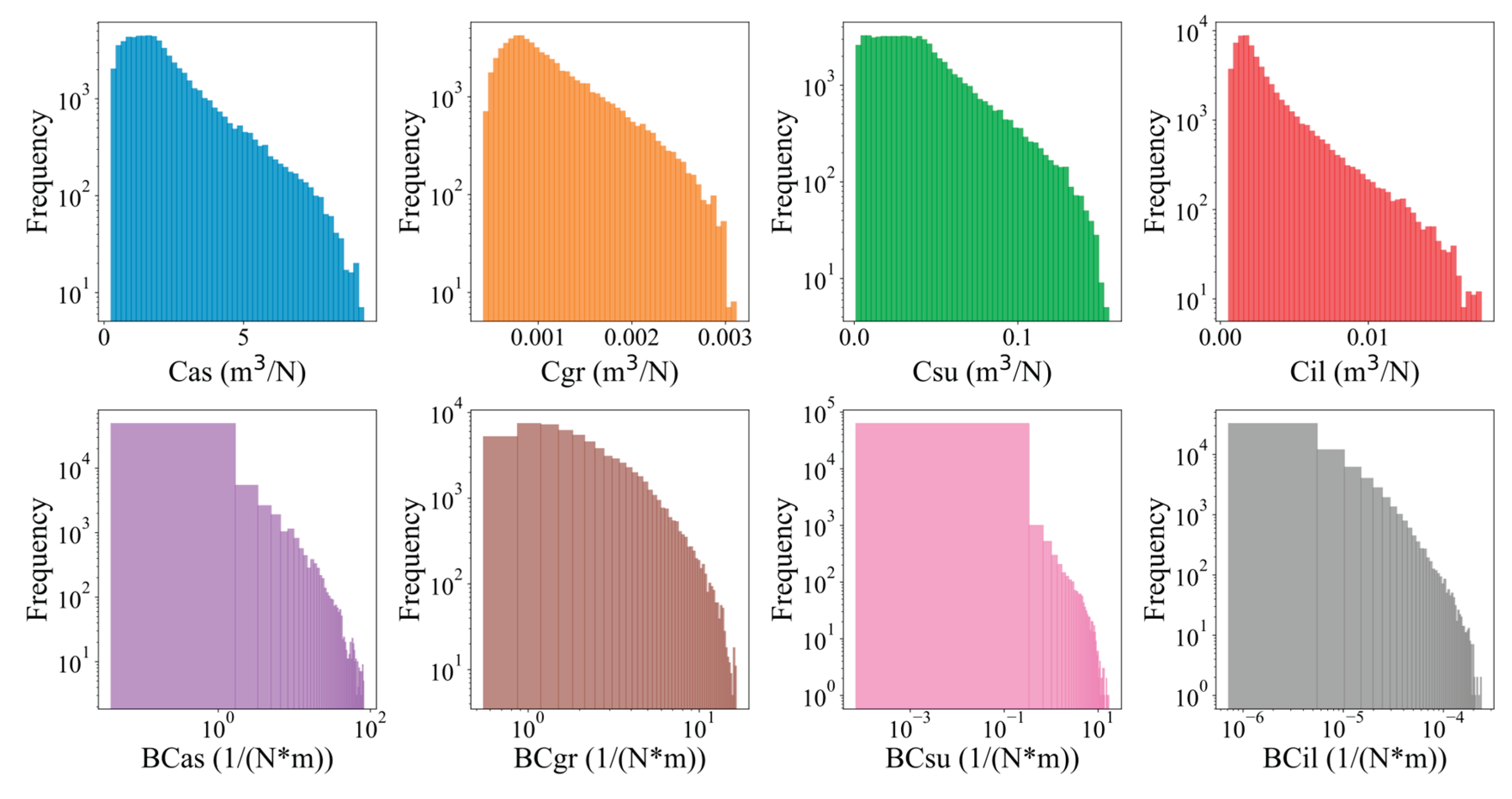
Figure 4.
Distribution of summary compliance SC and SBC.
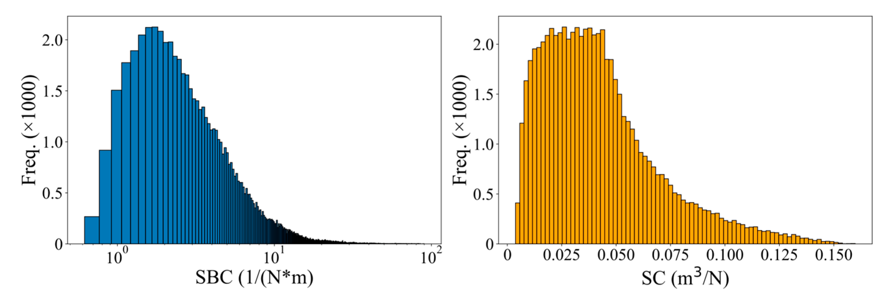
Figure 5.
Correlation matrix heatmap of deflection at measuring points.
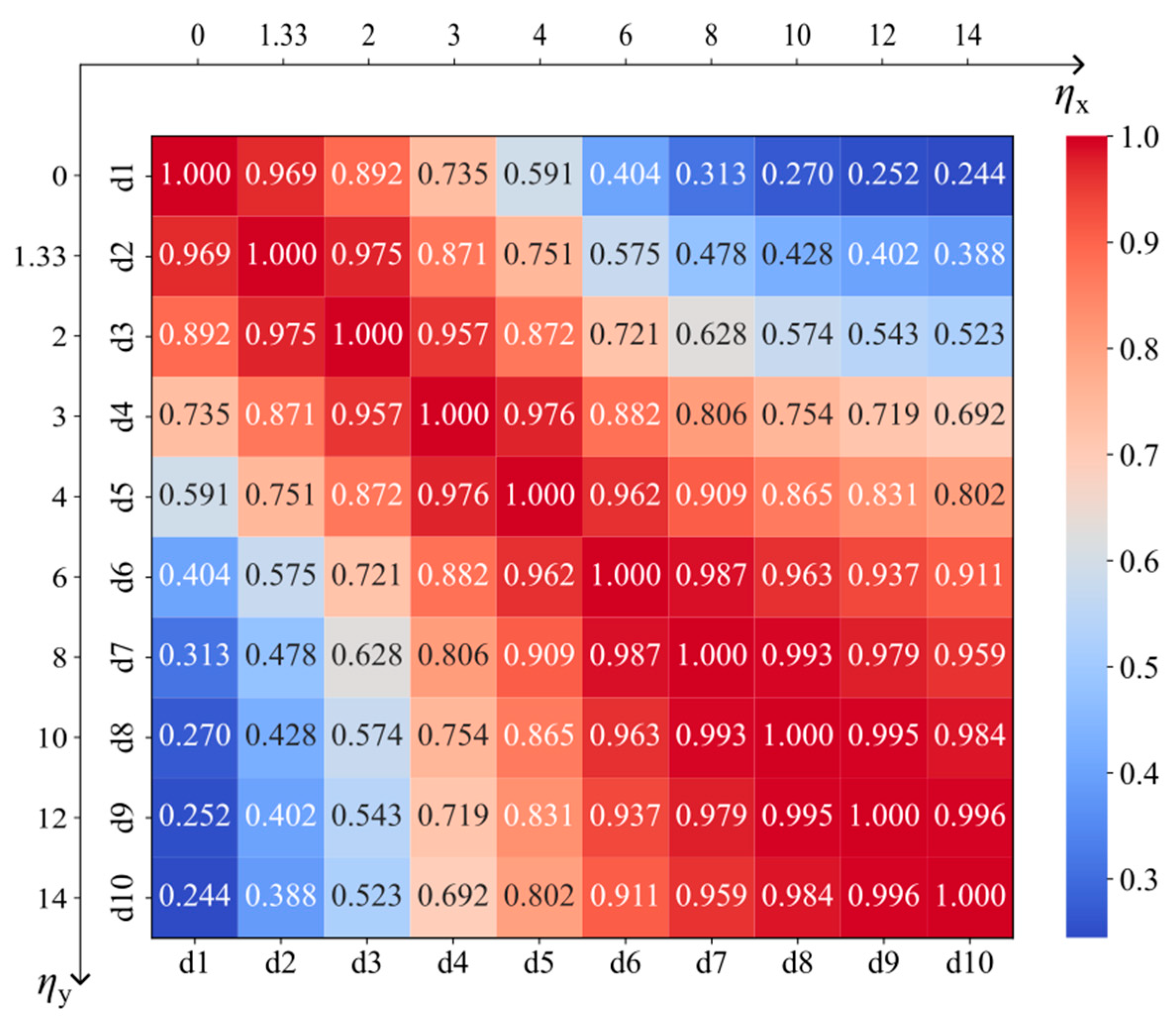
Figure 6.
Feature importance graph in terms of determining target parameters.
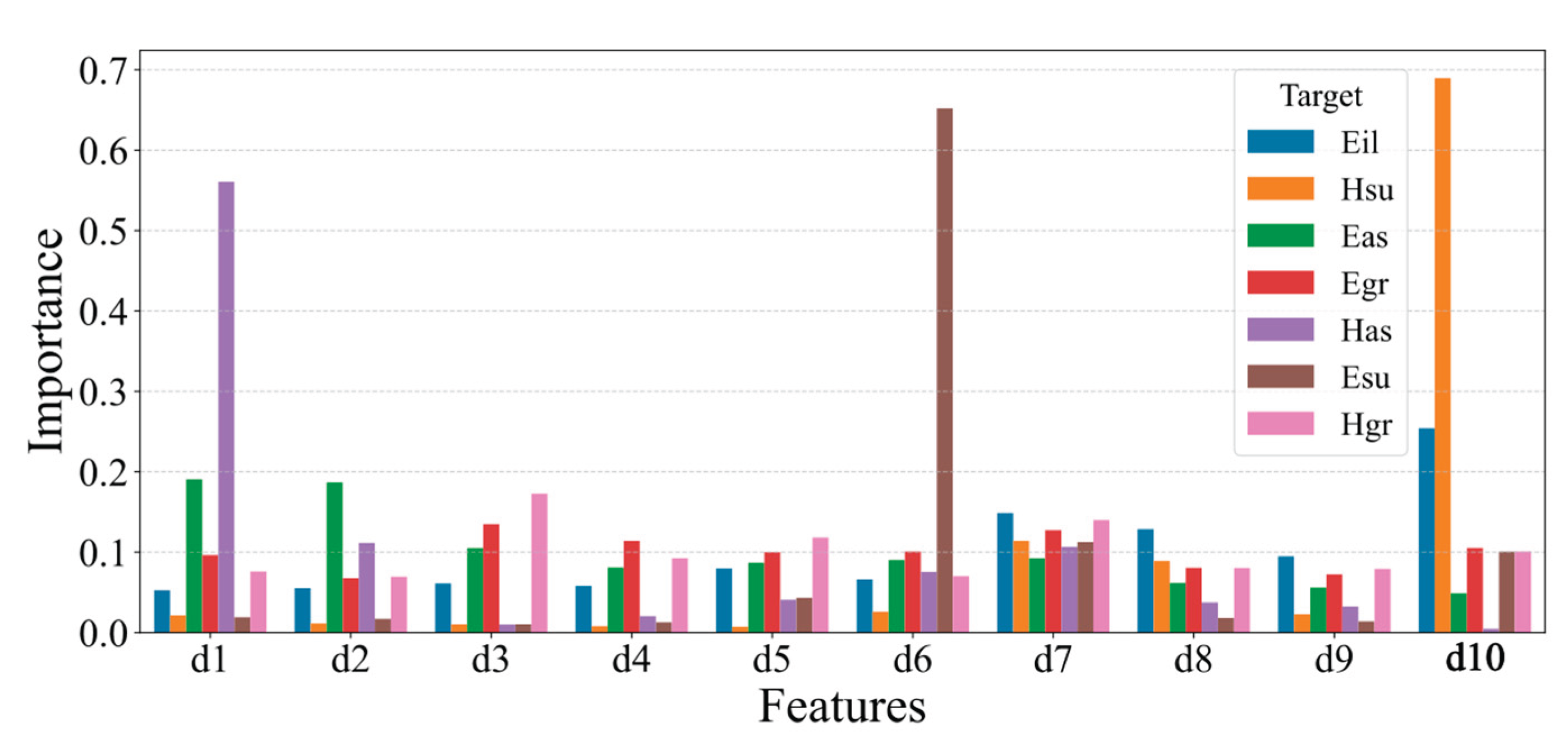
Figure 7.
SHAP violin plot for each target feature: (a) Has; (b) Hgr; (c) Hsu; (d) Eas; (e) Egr; (f) Esu; (g) Eil.
Figure 7.
SHAP violin plot for each target feature: (a) Has; (b) Hgr; (c) Hsu; (d) Eas; (e) Egr; (f) Esu; (g) Eil.
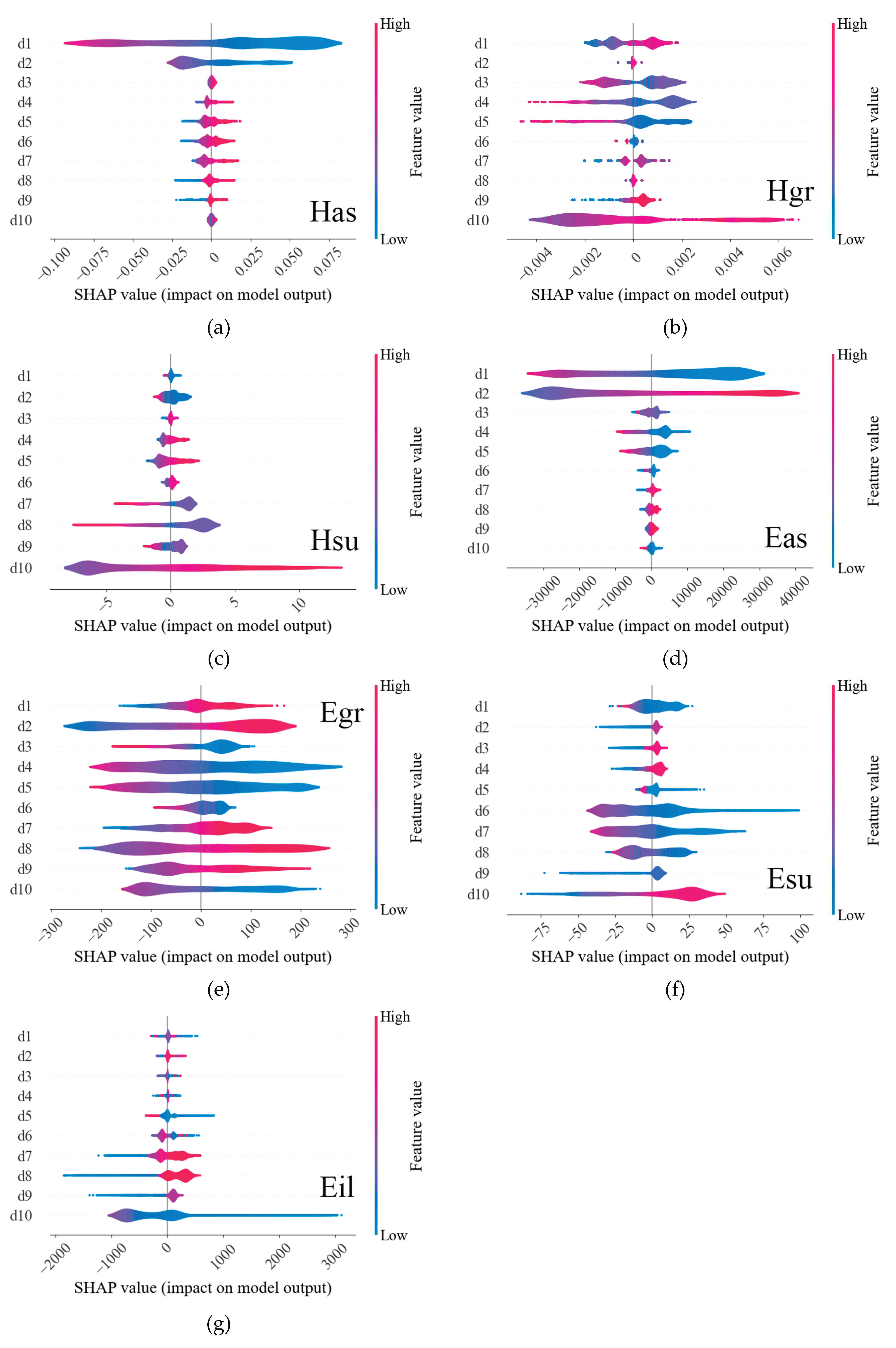
Figure 8.
Explained variance of each principal component.
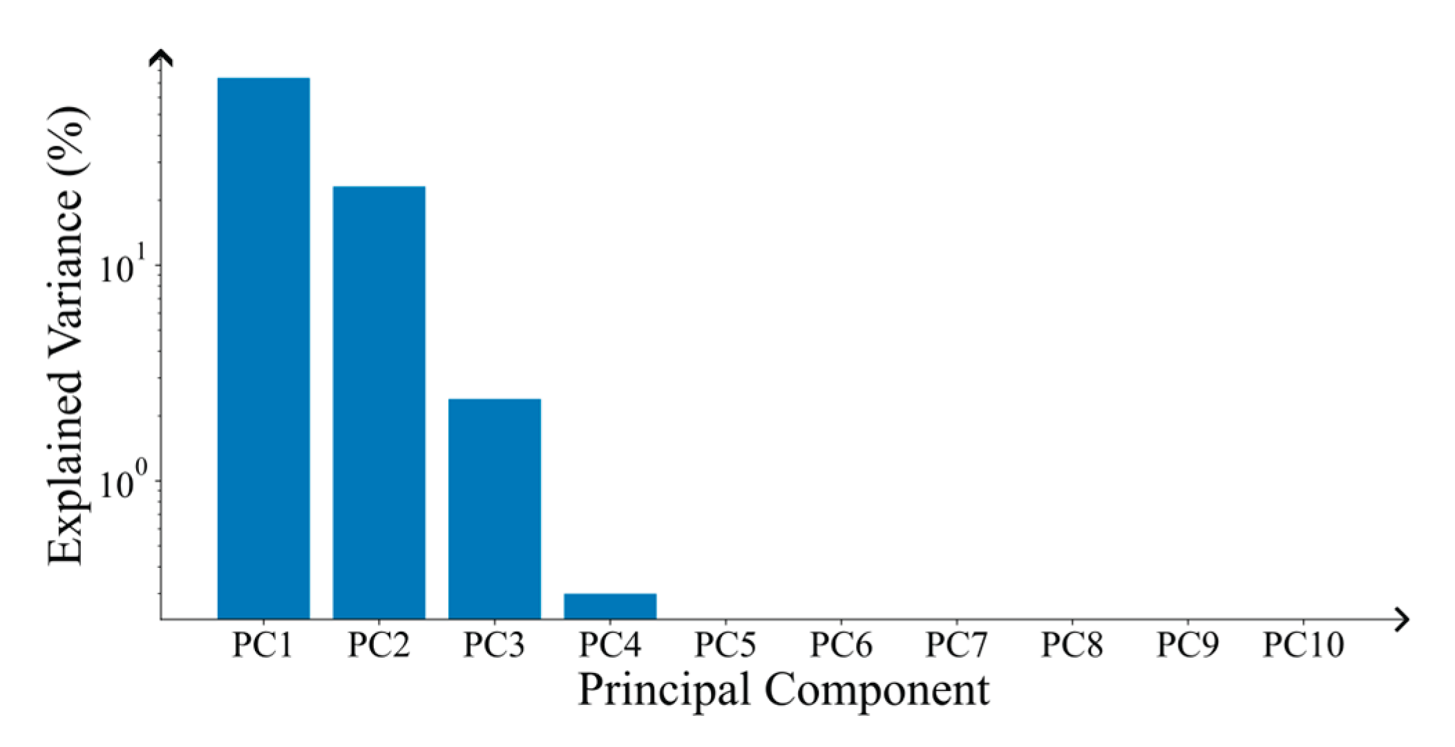
Figure 9.
Observations vs. predicted values of each model trained based on the database processed by PCA: (a) Has; (b) Hgr; (c) Hsb; (d) Eas; (e) Egr; (f) Esu; (g) Eil.
Figure 9.
Observations vs. predicted values of each model trained based on the database processed by PCA: (a) Has; (b) Hgr; (c) Hsb; (d) Eas; (e) Egr; (f) Esu; (g) Eil.
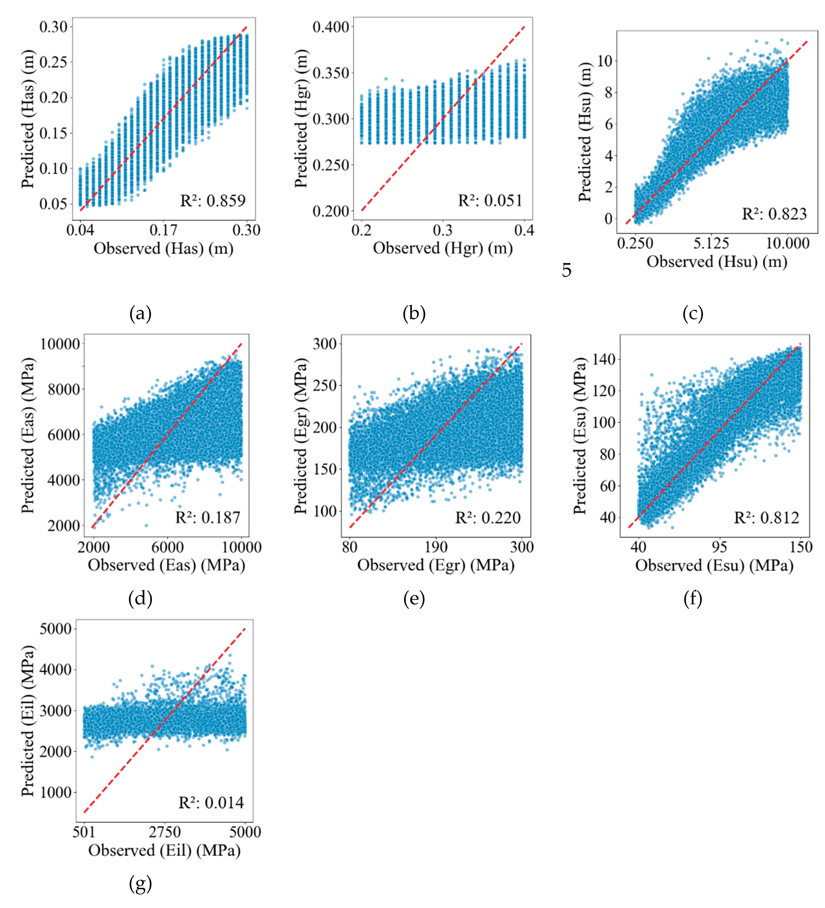
Figure 10.
Observations vs. residuals of each model trained based on the database processed by PCA: (a) Has; (b) Hgr; (c)Hsb; (d) Eas; (e) Egr; (f) Esu; (g) Eil.
Figure 10.
Observations vs. residuals of each model trained based on the database processed by PCA: (a) Has; (b) Hgr; (c)Hsb; (d) Eas; (e) Egr; (f) Esu; (g) Eil.
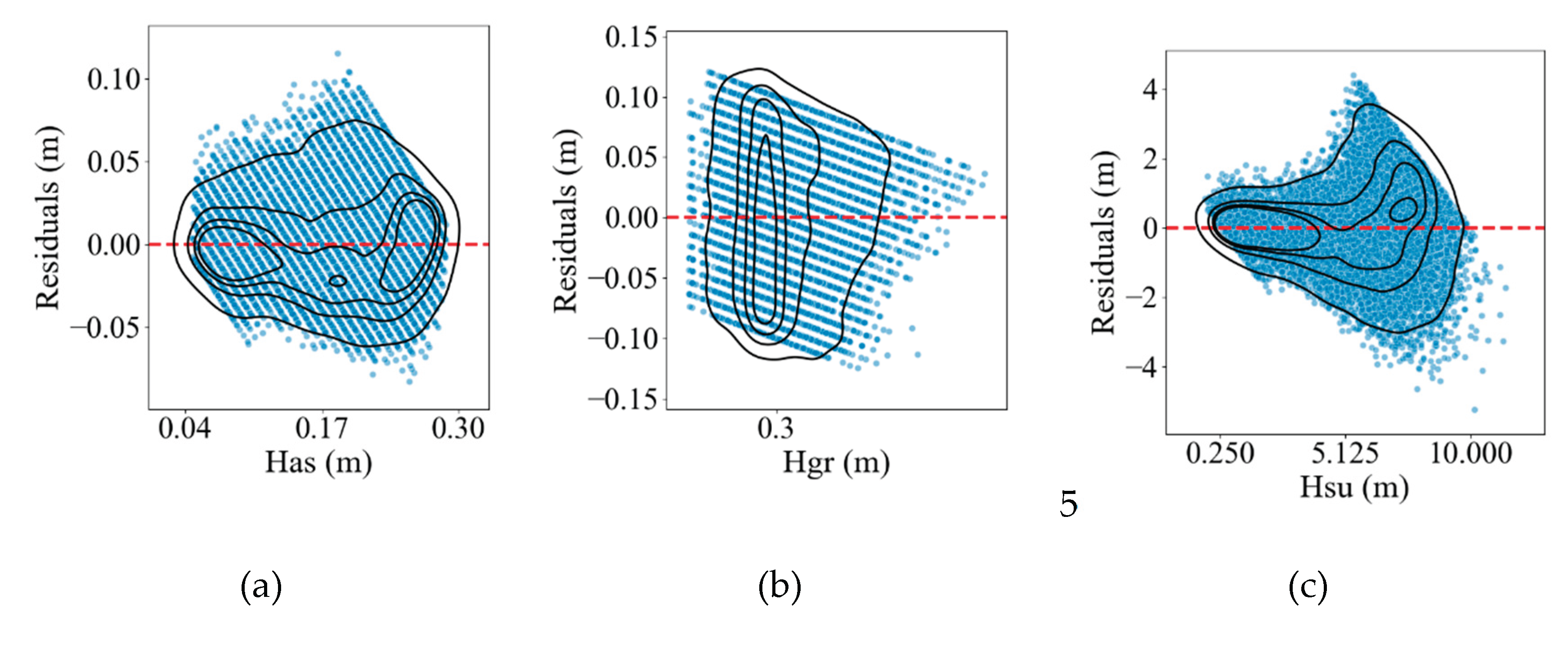
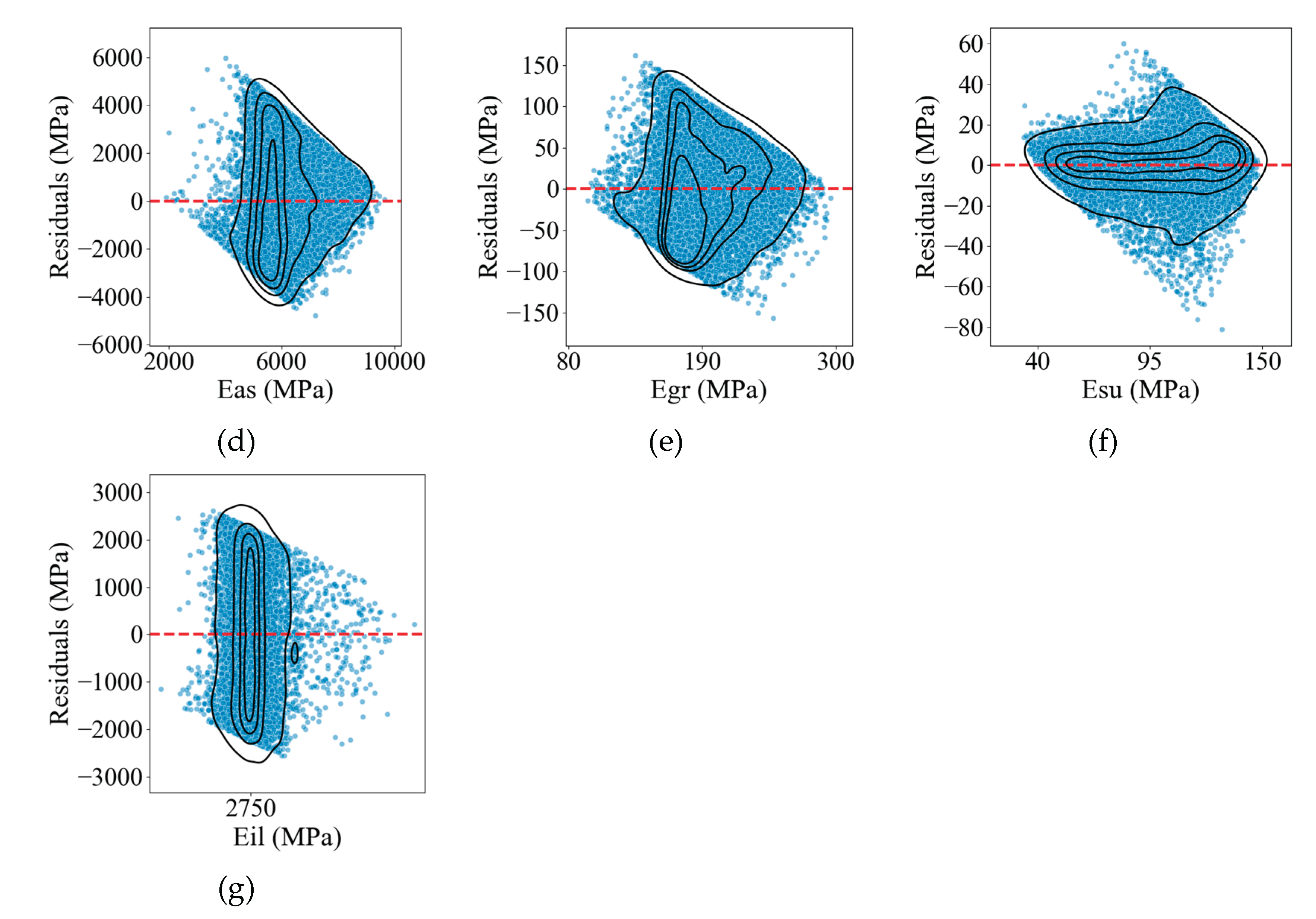
Figure 11.
Observations vs. predicted values of each model trained based on the database processed by FDM: (a) Has; (b) Hgr; (c) Hsu; (d) Eas; (e) Egr; (f) Esu; (g) Eil.
Figure 11.
Observations vs. predicted values of each model trained based on the database processed by FDM: (a) Has; (b) Hgr; (c) Hsu; (d) Eas; (e) Egr; (f) Esu; (g) Eil.
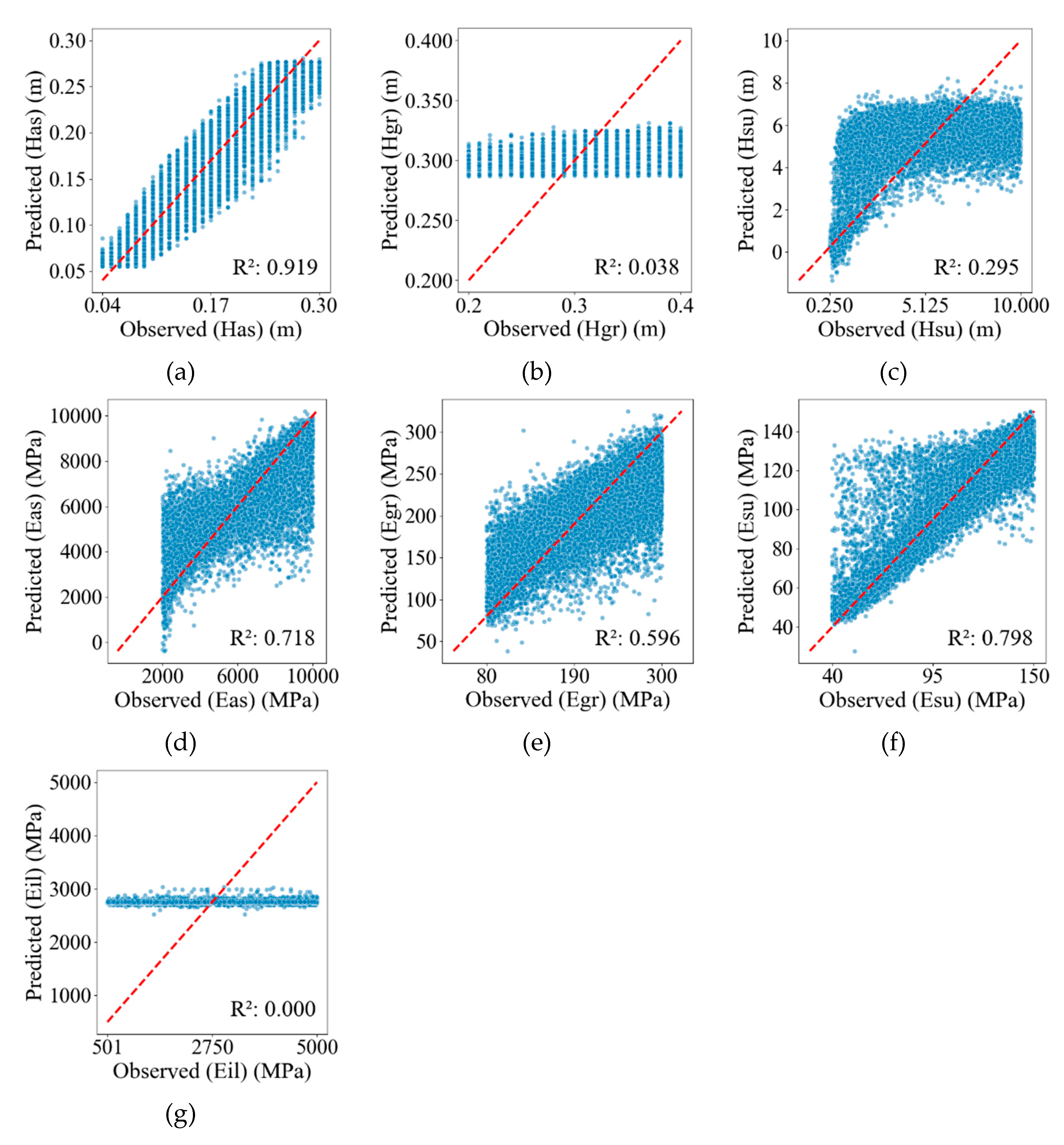
Figure 12.
Observations vs. residuals of each model trained based on the database processed by FDM: (a) Has; (b) Hgr; (c ) Hsu; (d) Eas; (e) Egr; (f) Esu; (g) Eil.
Figure 12.
Observations vs. residuals of each model trained based on the database processed by FDM: (a) Has; (b) Hgr; (c ) Hsu; (d) Eas; (e) Egr; (f) Esu; (g) Eil.
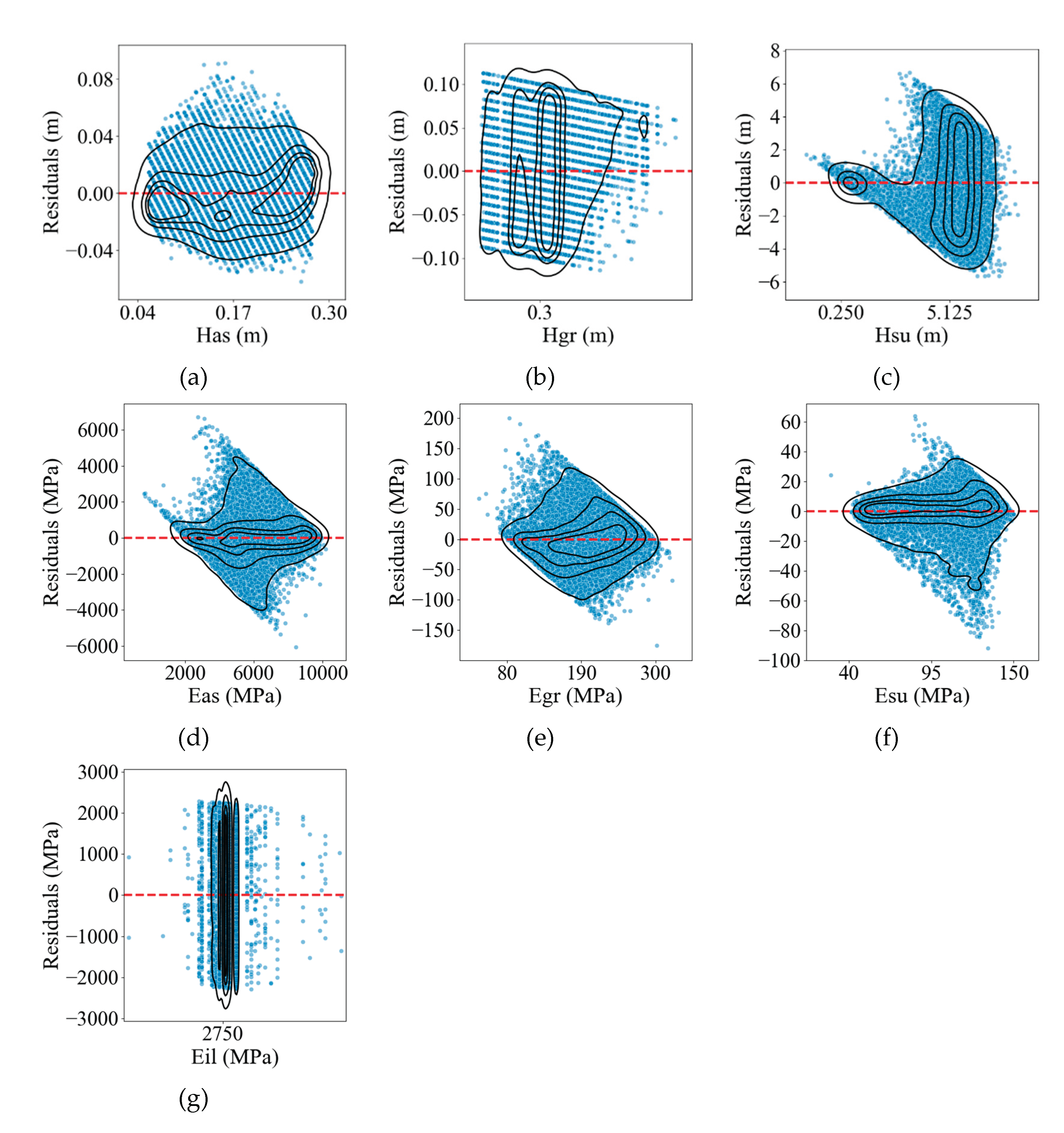
Table 1.
The range and interval of parameters used for data generation (UB- upper boundary, LB – lower boundary).
Table 1.
The range and interval of parameters used for data generation (UB- upper boundary, LB – lower boundary).
| Properties | Has(m) | Hgr(m) | Hsu(m) | Eas(MPa) | Egr(MPa) | Esu(MPa) | Eil(MPa) |
| UB | 0.04 | 0.2 | 0.25 | 2000 | 80 | 40 | 500 |
| LB | 0.3 | 0.4 | 10 | 10000 | 300 | 150 | 5000 |
| Interval | 0.001 | 0.001 | 0.01 | 1 | 0.1 | 0.1 | 1 |
Table 2.
Assessment of the database of deflections.
| Measuring Point |
Average (µm) |
Min. (µm) |
Max. (µm) |
Std. (µm2) |
Skewness | Kurtosis | (%) |
| d1 | 365.59 | 66.110 | 1658.0 | 189.97 | 1.36 | 2.21 | 3.24 |
| d2 | 289.65 | 51.790 | 1115.0 | 129.34 | 1.12 | 1.50 | 2.60 |
| d3 | 244.48 | 44.540 | 824.7 | 99.05 | 1.06 | 1.38 | 2.87 |
| d4 | 193.97 | 35.820 | 570.3 | 74.71 | 1.03 | 1.20 | 3.36 |
| d5 | 156.89 | 9.678 | 428.9 | 62.10 | 0.95 | 0.88 | 3.10 |
| d6 | 106.87 | -3.213 | 285.0 | 47.93 | 0.77 | 0.42 | 2.79 |
| d7 | 75.57 | -4.847 | 210.1 | 38.54 | 0.69 | 0.28 | 2.95 |
| d8 | 54.99 | -6.773 | 164.5 | 31.31 | 0.69 | 0.28 | 3.19 |
| d9 | 41.01 | -6.662 | 130.8 | 25.59 | 0.71 | 0.32 | 3.21 |
| d10 | 31.24 | -5.368 | 108.3 | 21.05 | 0.74 | 0.38 | 2.98 |
Table 4.
Evaluation of the model training for each target.
| Target | RMSE (m) | R2 | Target | RMSE (MPa) | R2 | |
| Has | 0.0276 | 0.860 | Eas | 1308.360 | 0.674 | |
| Hgr | 0.0575 | 0.0121 | Egr | 44.952 | 0.487 | |
| Hsu | 0.556 | 0.961 | Esu | 9.353 | 0.904 | |
| Eil | 1242.828 | 0.0842 |
Table 5.
Evaluation of the models trained based on the database processed by PCA.
| Target | RMSE (m) | R2 | Target | RMSE (MPa) | R2 | |
| Has | 0.027 | 0.862 | Eas | 2062.391 | 0.190 | |
| Hgr | 0.056 | 0.051 | Egr | 55.447 | 0.220 | |
| Hsu | 1.180 | 0.824 | Esu | 13.154 | 0.810 | |
| Eil | 1287.192 | 0.018 |
Table 6.
Evaluation of the models trained based on the database processed by FDM.
| Target | RMSE (m) | R2 | Target | RMSE (MPa) | R2 |
| Has | 0.0209 | 0.919 | Eas | 1225.3116 | 0.718 |
| Hgr | 0.0564 | 0.0376 | Egr | 39.9848 | 0.596 |
| Hsu | 2.3680 | 0.295 | Esu | 13.6717 | 0.798 |
| Eil | 1289.8261 | 0.0002 |
Table 7.
R2 of models trained by 3 different approaches.
| Targets | Whole dataset | PCA | FDM |
| Has | 0.860 | 0.862 | 0.919 |
| Hgr | 0.0121 | 0.051 | 0.0376 |
| Hsu | 0.961 | 0.824 | 0.295 |
| Eas | 0.674 | 0.19 | 0.718 |
| Egr | 0.487 | 0.22 | 0.596 |
| Esu | 0.904 | 0.81 | 0.798 |
| Eil | 0.0842 | 0.018 | 0.0002 |
Disclaimer/Publisher’s Note: The statements, opinions and data contained in all publications are solely those of the individual author(s) and contributor(s) and not of MDPI and/or the editor(s). MDPI and/or the editor(s) disclaim responsibility for any injury to people or property resulting from any ideas, methods, instructions or products referred to in the content. |
© 2025 by the authors. Licensee MDPI, Basel, Switzerland. This article is an open access article distributed under the terms and conditions of the Creative Commons Attribution (CC BY) license (http://creativecommons.org/licenses/by/4.0/).
Copyright: This open access article is published under a Creative Commons CC BY 4.0 license, which permit the free download, distribution, and reuse, provided that the author and preprint are cited in any reuse.


