Submitted:
25 October 2025
Posted:
27 October 2025
You are already at the latest version
Abstract
Given the urgent demand for flexible peak-shaving in power systems and underutilized distributed photovoltaic (PV) regulation potential, this paper proposes a distributed PV peak-shaving control strategy based on the temporal coupling self-organizing map (TC-SOM) neural network and a bi-level model. First, the SOM algorithm is improved for efficient feature extraction and accurate clustering of distributed PV data, realizing rational PV cluster division. On this basis, a bi-level peak-shaving model for distributed PV is constructed, forming a hierarchical peak-shaving mechanism from node demand to PV clusters to individual PVs to ensure inter and intra-cluster coordination. This hierarchical structure inherently embodies symmetry in response logic-realizing balanced interaction between upper-layer node demand guidance and lower-layer PV cluster/individual execution, as well as coordination control among different PV clusters. Case simulations and peak-shaving performance analysis on the IEEE-33 node system verify the strategy’s effectiveness: it significantly smooths the load curve, reduces peak-valley differences, and enhances distributed PV’s ability to participate in grid peak-shaving independently. This strategy provides strong support for precise regulation of distributed PV clusters and energy optimization in renewable dominant power systems, and is of great significance for promoting efficient and stable operation of power grids with high-proportion PV integration.
Keywords:
distributed photovoltaics
; cluster partitioning
; flexible peak shaving
; power symmetry
; TC-SOM
; bi-level model
1. Introduction
Against the backdrop of accelerating global energy transition and in-depth decarbonization, the power system is rapidly evolving toward high-proportion integration of new energy sources, with profound changes also occurring in user-side load characteristics [1]. In eco-nomically active and densely populated regions, improved terminal electrification and large-scale distributed energy integration have driven rapid electricity load growth while widening the load curve’s peak-valley difference [2,3]. For instance, a typical eastern China load center saw its maximum summer peak-valley difference expand by 42% in 2024 versus 2015. Australia saw its summer electricity peak-valley difference grow by approximately 45% in the 2022-2023 fiscal year compared to the 2018-2019 fiscal year, driven by soaring solar penetration and extreme heat-driven cooling demand [3,4]. This reflects the global challenge of growing peak-valley fluctuations, intensified grid regulation and power symmetry pressure under the integration of high-proportion renewable energy.
The traditional coal-fired power-dominated peak-shaving system faces dual pressures globally. Domestically, beyond 40% new energy penetration, its inherent intermittency unbalances regulation resources [5,6]; coal-fired units have limited deep peak-shaving capacity, physical storage is geographically constrained, and demand-side response remains immature [7,8,9]. Internationally, the International Energy Agency high-lights in its 2024 report that renewable energy integration in global power systems universally struggles with peak-shaving, as intermittent generation disrupts regulation resource balance even in mature markets [7]. Foreign studies, such as distributed cooperative control for microgrids [10] and hierarchical economic dispatch for hybrid energy systems [11], focus on multi-resource coordination but still fail to fully tap distributed PV’s standalone peak-shaving potential-mirroring domestic gaps. This urges the power industry worldwide to develop new peak-shaving technologies. Against this, distributed PV-with decentralized access and large-scale deployment [12]-has become a key system component. Meanwhile, policies in different countries stipulate that distributed photovoltaic systems must have the technical foundation of being "observable, measurable, adjustable, and controllable", and while ensuring local consumption, they shall reserve backup response capability to provide support for power grid security [13]. Its flexible temporal-spatial output and source-load coupling fill distribution network peak-valley gaps and cut losses [14], making it vital for easing peak-valley pressures under high new energy integration. Thus, studying distributed PV clustered management and precise regulation- to boost the system’s flexible peak-shaving and stability-has become a core power sector research direction.
In recent years, research on distributed PV cluster division and partitioning has attracted extensive attention from academia and industry. Existing studies mainly realize cluster partitioning based on geographical information, electrical characteristics, and operational data, using partitioning algorithms, optimization algorithms, and deep learning assistance [15]. Reference [5] applied the mGA-PSO optimization algorithm combined with the electrical distance between nodes to realize the cluster division of the distribution network, providing useful ideas for the division method based on electrical characteristics. Reference [16] used the K-means algorithm for multi-step grouping and equivalent modeling of distributed PV, and finally verified the rationality of cluster modeling. Reference [17] applied the network optimization community partitioning algorithm based on SLM-RBF to distributed PV scenario partitioning, effectively handling the uneven data distribution and improving the accuracy of scenario partitioning. However, existing studies rarely consider peak-shaving demand in the cluster division process, making it difficult to meet the actual needs of flexible peak-shaving in power systems. On the other hand, distributed PV systems are characterized by high complexity and many variables, and traditional partitioning methods often face problems such as low computational efficiency and poor partitioning accuracy when processing high-dimensional data. Therefore, there is an urgent need for a high-performance method suitable for processing high-dimensional data to achieve accurate di-vision and partitioning of distributed PV clusters.
Based on cluster partitioning research, distributed PV clusters can participate in grid peak-shaving as a unified cluster entity. However, Existing studies have shown that the coordinated control methods for distributed PV clusters participating in grid peak-shaving have defects such as low coordination efficiency and insufficient global optimization capability [18]. Current research on distributed PV cluster participation in grid peak-shaving control strategies mainly focuses on the coordinated peak-shaving strategies of distributed PV with multiple resources such as energy storage and conventional units [19]. Reference [11] proposed that energy storage-assisted grid peak-shaving has obvious advantages. In different time periods, the grid load varies greatly. Energy storage can be charged during low load and discharged during high load, thereby reducing the peak-valley difference of the grid to meet peak-shaving needs. Reference [10] established an "aggregation-peak shaving-decomposition" model containing a high proportion of PV and energy storage. Studies have shown that the use of PV and energy storage resources can alleviate the peak-shaving pressure of the power system and achieve better economic benefits under the premise of ensuring peak-shaving capability. However, the above studies mainly focus on the coordinated peak-shaving strategies of distributed PV with other equipment, lacking in-depth research on the peak-shaving capability of distributed PV itself, which results in distributed PV resources still being in a supporting role in the grid peak-shaving system, and their flexible adjustment potential and cluster synergy value need to be systematically explored. At the same time, due to the geographical dispersion of distributed PV and the characteristics of grid end access, traditional peak-shaving control strategies face problems such as high communication delay, high solution dimension, and limited control real-time performance.
To address the above issues, this paper proposes a distributed PV cluster partitioning and flexible peak-shaving strategy based on temporal coupling SOM and bi-level model driving. The strategy first improves the SOM algorithm, adopts a two-stage division structure, improves the similarity measurement method, and verifies the effectiveness of cluster division, thereby achieving efficient feature extraction and accurate partitioning of distributed PV data to realize reasonable division of PV clusters. On this basis, a bi-level model is constructed to form a hierarchical peak-shaving mechanism from node demand to PV clusters and then to individual distributed PV. The upper model calculates the scheduling distance ac-cording to the system node load disturbance and dynamically allocates peak-shaving tasks to each cluster. The lower model controls the output of each PV unit in proportion based on the remaining output capacity of distributed PV within the cluster, ensuring effective collaboration between clusters and among distributed PV units. Finally, through case simulation and peak-shaving performance analysis of the IEEE-33 node system, the effectiveness and feasibility of the proposed method in scenarios where a high proportion of distributed PV participates in flexible peak-shaving of the power system are verified.
2. Distributed Photovoltaic Cluster Partitioning Based On TC-SOM
Considering the characteristics of distributed photovoltaics such as wide distribution area, scattered lo-cations, large quantity, and small individual capacity, directly incorporating them into the operation and control framework of the power system will lead to problems such as a significant increase in solution complexity and high dimensionality of decision variables [20]. Therefore, this paper aggregates PV resources with adjacent geographical locations and close electrical connections into cluster units through a partitioning approach, and establishes a hierarchical collaborative control architecture to realize cluster-level optimal scheduling and coordinated control of distributed PV [21]. This paper proposes a method for distributed PV cluster partitioning and flexible peak shaving based on temporal coupling SOM and a Bi-level model, whose overall framework is shown in Figure 1.
Under the above framework, the comprehensive indicators for distributed PV cluster partitioning used in this paper can be divided into three categories according to their characteristics, namely electrical coupling, power balance capability, and temporal characteristics. Electrical coupling focuses on considering the degree of electrical association between nodes within a cluster and between clusters, so as to better evaluate the integrity and synergy of the clusters; power balance capability calculates the power balance level of each PV cluster and individual PV when participating in peak shaving, providing a numerical basis for the next step of distributed peak shaving; temporal characteristics are used to measure the output variation rules and complementarity of PV clusters in different time periods, and according to the temporal characteristics of the clusters, corresponding peak shaving tasks can be is-sued to each cluster.
2.1. Partition Index
The electrical coupling index is used to measure the strength of electrical association between clusters, and is comprehensively evaluated using reactive power sensitivity, electrical distance, and node topological connection strength. Among them, reactive power sensitivity represents the degree of influence of load node power changes on voltage changes of other nodes, and its expression is given by Equation (1):
where S is the sensitivity matrix, indicating the response of node voltage changes to load node power changes; electrical distance reflects the tightness of electrical connections between nodes, where is the ratio of voltage fluctuations between the node itself and related nodes when reactive power fluctuates.
By employing the sensitivity matrix, the relationship between a node’s own voltage fluctuation and the resulting voltage fluctuations at surrounding nodes can be obtained, from which an electrical-distance expression is derived.
Define the topological connection strength T between node i and node j as the reciprocal of the shortest path length between the two nodes:
The comprehensive electrical coupling indicator E is calculated as .
Define the net load at time t as:
where is the system load at time t, and is the self-consumed output of distributed PV at time t.
The power balance capability is measured by indicators such as the net load ramp rate and load factor. The net load ramp rate represents the rate of change of net load per unit time, reflecting the intensity of load changes, and its expression is as follows:
where and are the net loads at time t and t+1 respectively, and is the time interval.
The load factor refers to the ratio of the actual output of a photovoltaic cluster to its maximum possible out-put, reflecting the output utilization level of the photovoltaic cluster. In the calculation, it is necessary to real-time monitor the actual power generation of the photovoltaic cluster and combine it with the maximum generating power under the meteorological conditions of the day, which reflects the output utilization level of the photovoltaic cluster. Its expression is as follows:
where is the actual output of the photovoltaic cluster, and is the maximum possible output.
The comprehensive power balance capability indicator P is calculated as .
The output curve correlation coefficient is calculated based on the Pearson correlation coefficient, which quantifies the linear correlation between the output sequences of two PV clusters over a continuous time period. For two PV clusters with output sequences and , the covariance and standard deviations , are first calculated:
where and are the average outputs of the two clusters, respectively.
The output curve correlation coefficient is shown in Equation (11) of this paper:
Finally, the comprehensive cluster partitioning index is generated by combining the electrical coupling, power balance capability, and temporal characteristic indicators as follows:
2.2. Adaptive SOM Algorithm
Distributed photovoltaic cluster partitioning is based on multi-dimensional features such as the geographical location, output characteristics, and meteorological data of distributed photovoltaics. It uses partitioning algorithms to extract and group features, dividing photo-voltaic power plants with similar output patterns and close electrical connections into the same cluster, so as to achieve large-scale management and coordinated peak-shaving control. As an unsupervised learning method, the Self-Organizing Map neural network has shown unique advantages in fields such as data dimensionality reduction, feature extraction, and visualization [22], and is very suitable for cluster partitioning of distributed photovoltaics. The core idea of the traditional SOM is to map high-dimensional input data to a low-dimensional topological structure through competitive learning while maintaining the topological relationship between data. The topological structure of the traditional SOM is shown in Figure 2.
The SOM algorithm takes the aforementioned com-prehensive cluster partitioning indicators of distributed photovoltaics as input, and obtains a distance set by calculating the Euclidean distance between each input layer data and the competitive layer neurons, specifically as shown in Equation (13):
where is the comprehensive cluster partitioning indicator data of the i-th node, and represents the connection strength between the i-th neuron in the input layer and the j-th neuron in the competitive layer, which initially takes a small value. The minimum distance is selected from the obtained distance set, and the competitive layer neuron represented by this distance is the winning neuron. The weight vectors of the winning neuron and the neurons in its neighborhood will be updated according to the rules calculated by Equation (14):
where is the learning rate, which gradually de-creases with the training time t and controls the step size of weight update; is the neighborhood function, which centers on the winning neuron and gradually reduces the neighborhood range with the training time. Its role is to make the weight vectors of the winning neuron and its surrounding neurons move towards the direction of the input vector, thereby forming a topo-logical representation of the input photovoltaic data distribution in the competitive layer. The neighbor-hood function usually adopts the form of a Gaussian function:
where and are the positions of the winning neuron c and the neuron j in the competitive layer respectively, and is the neighborhood width, which also gradually decreases with the training time t.
However, traditional SOM has certain limitations in processing complex data of distributed photovoltaics, making it difficult to fully consider the comprehensive impact of electrical coupling, power balance capability, and temporal characteristics. Therefore, this paper proposes a TC-SOM model, which improves the partitioning effect through a two-stage division structure, improved similarity measurement, and verification of cluster division effectiveness. The two-stage division structure is specifically divided into the electrical coupling layer and the power timing layer. The TC-SOM topology map is shown in Figure 3.
Among them, the input of the first-stage rough partitioning includes reactive power sensitivity, electrical distance, and node topological connection strength. The goal of this stage is to divide nodes with close electrical connections into the same initial cluster, using a low-dimensional mapping structure. By calculating the similarity of input indicators, nodes with high similarity are mapped to adjacent neuron positions, achieving close electrical coupling within the cluster. The second-stage fine partitioning is carried out on the basis of rough partitioning, with inputs including net load climbing rate, output curve correlation coefficient, and load rate, and a high-dimensional mapping structure is adopted. Through the analysis of these indicators, the power timing complementarity within the cluster is realized, so that the photovoltaic output within the same cluster can complement each other in time, improving the overall peak-shaving capability.
In terms of similarity measurement, dynamic weighted Euclidean distance is used to calculate the similarity between input data and neuron weights. Different weights are assigned according to the importance of different indicators in partitioning, and the weight values are dynamically adjusted based on data characteristics. For the electrical coupling layer, reactive power sensitivity, electrical distance, and node topo-logical connection strength have larger weights; for the power timing layer, net load climbing rate, output curve correlation coefficient, and load rate have larger weights. The expression for dynamic weighted Euclidean distance is:
where is the weight of the i-th indicator, and and are the i-th indicator values of the input data and neuron weights, respectively.
For the verification of cluster division effectiveness, evaluation indicators such as inter-cluster tie-line power fluctuation rate, intra-cluster self-balancing rate, and climbing flexibility deficit are adopted. Among them, the inter-cluster tie-line power fluctuation rate reflects the fluctuation of power on the tie-lines between different clusters; the smaller the fluctuation rate, the more reasonable the cluster division and the smaller the mutual influence between clusters. The intra-cluster self-balancing rate represents the proportion of power that can be self-balanced within the cluster to the total power; the higher the self-balancing rate, the better the independence and stability of the cluster. The climbing flexibility deficit measures the degree of insufficient flexibility of the cluster in responding to load climbing; the smaller the deficit, the stronger the climbing capacity of the cluster and the better it can meet the peak-shaving demand.
2.3. Overall Steps
Based on the above-mentioned temporal coupling SOM algorithm, combined with three types of key parameters including electrical coupling, power balance capability, and temporal characteristics, the division scheme for each cluster is determined, and the specific process is shown in Figure 4. Through the two-stage division structure, hierarchical partitioning processing of data is realized, and the accuracy of cluster partitioning is improved. Finally, through the visualized partitioning results, the load cluster partitioning results are output, with the specific steps as follows:
Step 1: Establish a multi-dimensional evaluation index system based on three types of key parameters, namely electrical coupling, power balance capability, and temporal characteristics. Eliminate dimensional differences through standardization to form a feature data input set.
Step 2: Perform the first-stage rough. Input reactive power sensitivity, electrical distance, and node topo-logical connection strength into the low-dimensional mapping SOM network to realize the initial partitioning of nodes with close electrical connections.
Step 3: On the basis of the rough partitioning results, perform the second-stage fine partitioning. Input the net load climbing rate, output curve correlation coefficient, and load rate into the high-dimensional mapping SOM network, and calculate the similarity through dynamic weighted Euclidean distance to realize fine partitioning of power timing complementarity within the cluster.
Step 4: Verify the effectiveness of the division results using indicators such as inter-cluster tie-line power fluctuation rate, intra-cluster self-balancing rate, and climbing flexibility deficit. Generate a load cluster partitioning map in combination with visualization analysis tools, and finally output the cluster optimization scheme that meets the peak-shaving demand.
3. Bi-Level Model Architecture for Flexible Peak-Shaving of Distributed Photovoltaics
Bi-level control model achieves collaborative management of complex systems based on a hierarchical architecture. The upper layer focuses on global situation analysis and strategy formulation, while the lower layer specializes in localized command execution and re-al-time adjustment. The two form a dynamic closed loop through bidirectional information interaction. This structure not only retains the rapid response characteristics of distributed control but also enhances the overall coordination capability of the system through inter-layer collaborative optimization, ensuring the autonomy of each unit while effectively achieving global objectives.
3.1. Bi-level Framework
The distributed photovoltaic peak-shaving Bi-level control model proposed in this paper realizes coordinated control through a hierarchical response strategy. The upper-layer system dynamically allocates peak-shaving tasks according to load disturbances, while each photovoltaic cluster in the lower layer adjusts their output in a differentiated manner based on the degree of correlation with disturbance nodes. Be-tween the upper and lower layers, cluster peak-shaving demands and the existing output of distributed photovoltaics serve as an interaction bridge, ultimately achieving distributed photovoltaic peak-shaving control Figure 5.
The upper-level optimization model calculates the dispatch distance between the disturbance node and each distributed photovoltaic cluster based on system node load disturbances, and determines the overall output adjustment amplitude of each cluster in response to load fluctuations according to the magnitude of the dispatch distance. The dispatch distance derived from node sensitivity is shown in Equation (17).
where is the sensitivity ratio from node i in cluster m to the disturbance node; is the average sensitivity of all nodes in cluster m.
Clusters with a shorter dispatch distance respond more directly to load disturbances, so their output adjustment amplitude is relatively larger. In contrast, clusters with a longer dispatch distance adjust their output accordingly based on their relationship with the disturbance node to jointly achieve the peak-shaving effect. This process is coordinated and optimized through an optimization algorithm to ensure that the output adjustments of each cluster can effectively sup-press load fluctuations, thereby achieving the goal of peak-shaving.
On the basis of determining the total output of each cluster, each cluster allocates and controls the output of each distributed photovoltaic unit according to the remaining output capacity of each PV unit under the maximum power point tracking state, in proportion to their remaining capacities, as specifically shown in Equation (18):
where is the power variation of the load at the disturbance node; M is the total number of photovoltaic clusters; is the peak-shaving power command allocated to the m-th cluster.
This control method ensures that while meeting the overall output requirements of the cluster, the actual output capabilities of each distributed photovoltaic unit are fully considered, avoiding situations where the stability and efficiency of the entire system are affected due to over-limited output of individual PV devices. Through this output control based on the proportion of remaining capacity, the lower-level control of distributed PVs is realized, enabling each PV unit to flexibly adjust its output according to its own status and capabilities, thereby improving the peak-shaving capacity and energy utilization efficiency of the entire cluster.
3.2. Upper-level Optimization Model
The upper-level model constructs a comprehensive objective function to optimize the performance of dis-tributed PV in power system peak-shaving. The specific implementation process is shown in Figure 6.
The core objectives of this function are to minimize the difference between peak and valley values of the post-regulation nodal load curve, maximize the utilization efficiency of PV peak-regulation capacity, and enhance the response flexibility of distributed PV clusters. By optimizing the output of distributed PVs, the amplitude of nodal load fluctuations is reduced, thereby decreasing the peak-valley difference. Mean-while, ensuring full utilization of PV peak-regulation capacity improves energy efficiency, while enhancing the response flexibility of each cluster enables quicker adaptation to load changes, thus improving the stability and flexibility of the power system in the face of load fluctuations.
where and respectively represent the maximum and minimum values of nodal load fluctuations; denotes the peak-valley difference; represents the photovoltaic output of the i-th cluster without peak-shaving; is the photo-voltaic output of the i-th cluster after peak-shaving optimization; indicates the remaining value of photovoltaic peak-shaving capacity; and are the costs of increasing and decreasing photovoltaic output, respectively; and are the output increased or decreased at time t; and is the cost of photovoltaic peak-shaving.
Equation quantifies the flexible response capability of a cluster. A larger cumulative deviation area indicates better response performance, whereas a smaller cumulative deviation area indicates poorer response performance. The expression is given below:
where T is the simulation period; is the cluster’s net load at time t; is the cluster’s actual power output at time t; is the adjusted response deviation area, representing the cumulative magnitude of the difference between the cluster’s output and its net load over the interval [0, T]; is the cluster’s initial net load; is the aggregate active-power output of all generators inside the cluster when no regulation is ap-plied; is the baseline response deviation area obtained in the absence of any regulation.
3.3. Lower-level Control Model
The lower-level control focuses on the output adjustment of each distributed photovoltaic unit itself, and in actual operation, it is necessary to consider many operational constraints of the overall system. Since the power generation capacity of PV units is significantly affected by environmental factors such as illumination intensity and temperature, there exist minimum and maximum output values. Therefore, the actual output of distributed PVs must be restricted within their own adjustable range. the specific implementation process is shown in Figure 7.
Meanwhile, to avoid sharp fluctuations in the output of PV units that may impact the power grid, their ramp capability constraints also need to be considered. Specifically, the output variation amplitude of PV units at adjacent time instants must not exceed their maximum ramp rate, ensuring a smooth transition of PV output.
The output constraints of PV units are as shown in the following equation:
Where , and are the maxi-mum values of the reliable upward and downward regulation capacities of each photovoltaic cluster m, respectively.
The entire distribution network must satisfy real-time power balance at all times during operation. That is, the total load borne by the system equals the sum of the total output of all distributed photovoltaic clusters and the output of thermal power units. This avoids problems such as insufficient power supply caused by power shortages and energy waste caused by power surpluses, and maintains the stable operation of the power system. The overall energy balance constraint of the system is as follows:
where , and respectively represent the load, the output of thermal power units, and the total output of photovoltaic clusters.
Power grid security constraints include voltage constraints and line power constraints. Voltage constraints require that the voltage at each node must be maintained within the allowable range. Line power constraints, on the other hand, specify that the transmission power of each line must not exceed its capacity limit. Each line has a designed maximum transmission capacity to maintain the safe operation of the power grid. The system security constraints are as follows:
where and respectively denote the voltage at node i and the power flow on node i to node j.
Lower-level control, through the aforementioned multi-dimensional constraints, maximizes the tapping of PV peak-shaving potential on the premise of ensuring stable grid voltage and controllable line power. It has formed a collaborative control mechanism from individual equipment to the global system, providing underlying technical support for the engineering implementation of the bi-level model.
3.4. Implementation of the Coordinated Peak-shaving Strategy
The coordinated peak-shaving strategy realizes dynamic coordinated control between distributed photo-voltaic clusters and load disturbances through hierarchical task decomposition and a closed-loop feedback mechanism. This strategy takes dispatch distance as the basis for task allocation, and remaining peak-shaving capacity as the foundation for underlying regulation, improving peak-shaving efficiency and system stability through bi-level linkage. The specific implementation steps are as follows:
Figure 8.
Flowchart of distributed photovoltaic peak shaving based on bi-level model
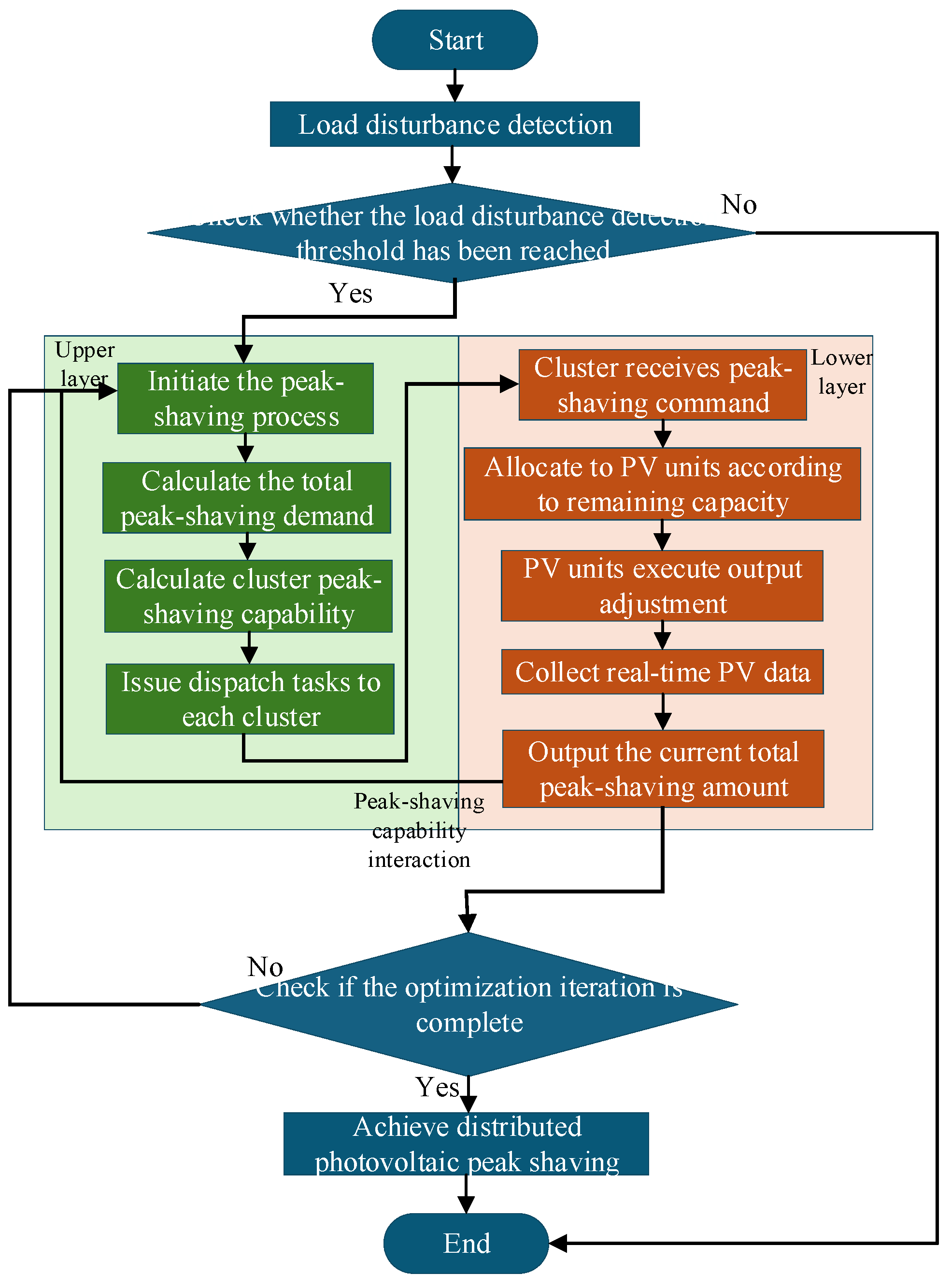
Step 1: When the system detects a load disturbance, the upper-level model first calculates the dispatch distance between each photovoltaic cluster and the disturbance node. Based on the inverse proportion of dispatch distances, the upper-level model allocates the total peak-shaving demand of the system to each cluster. Clusters with shorter dispatch distances undertake the main peak-shaving tasks, while those with longer distances provide auxiliary support, achieving differentiation and efficiency in task allocation.
Step 2: After receiving peak-shaving commands, each cluster performs secondary allocation according to the remaining peak-shaving capacity of internal photovoltaic units. Photovoltaic units with larger remaining capacities undertake greater output adjustment amounts. This allocation method ensures that photo-voltaic units respond to peak-shaving demands within their adjustable range, avoiding overload.
Step 3: The lower level feeds real-time output data back to the upper-level model, which updates the dis-patch distances of each cluster and the evaluation of their peak-shaving capabilities based on the feedback information. Through the closed-loop mechanism of bi-level coordination, it adapts to the temporal and spatial output variation characteristics of distributed photovoltaics, continuously improving the accuracy and robustness of the peak-shaving strategy.
4. Case Study
4.1. Case System
To verify the feasibility and effectiveness of the proposed distributed photovoltaic cluster partitioning and coordinated peak-shaving strategy in this paper, the IEEE-33 node system is selected for simulation analysis. This system has a radial topology, consisting of 33 nodes and 32 branches [23]. It features a moderate number of nodes, clear structure, and the ability to flexibly simulate various operating scenarios, effectively replicating complex working conditions such as load fluctuations and distributed generation integration in real distribution networks. This provides a model basis for testing the partitioning accuracy and peak-shaving strategy effectiveness under high penetration of distributed photovoltaics. By constructing scenarios with high penetration of distributed photovoltaics in this system, the adaptability and reliability of the proposed method under different load disturbance conditions can be comprehensively evaluated. Its specific topology is shown in Figure 9.
In the IEEE-33 node system, 11 nodes are selected as access points for distributed photovoltaics. By adding distributed photovoltaics at these nodes, a case scenario with high-penetration distributed photovoltaic integration is constructed, so as to analyze and study the system performance under this condition. The specific access points are shown in Table 1.
In terms of data collection, it is simulated and set that the sampling frequency of distributed photovoltaic output and related environmental data at each node is once per hour, so as to ensure the timeliness and accuracy of the data and provide a reliable basis for subsequent cluster partitioning. The simulation platform is built in the Python environment, making full use of its abundant library resources. Meanwhile, combined with the Matplotlib library, data visualization display is performed on the partitioning results of distributed photovoltaic clusters, so as to more intuitively present the performance and partitioning effect of the algorithm.
4.2. Partitioning of Distributed PV Clusters
After the integration of high-proportion distributed photovoltaics, the improved SOM algorithm is adopted to conduct cluster partitioning on the parameters of this 33-node model. Based on the scheduling distance index, peak shaving capacity index and response sensitivity index mentioned above, cluster analysis and cluster division are performed on the data of each node in the system. After learning and screening through the multi-layer SOM neural network, the final three-layer division results obtained are shown in the figure below.
Figure 10.
Partitioning results of TC-SOM structure
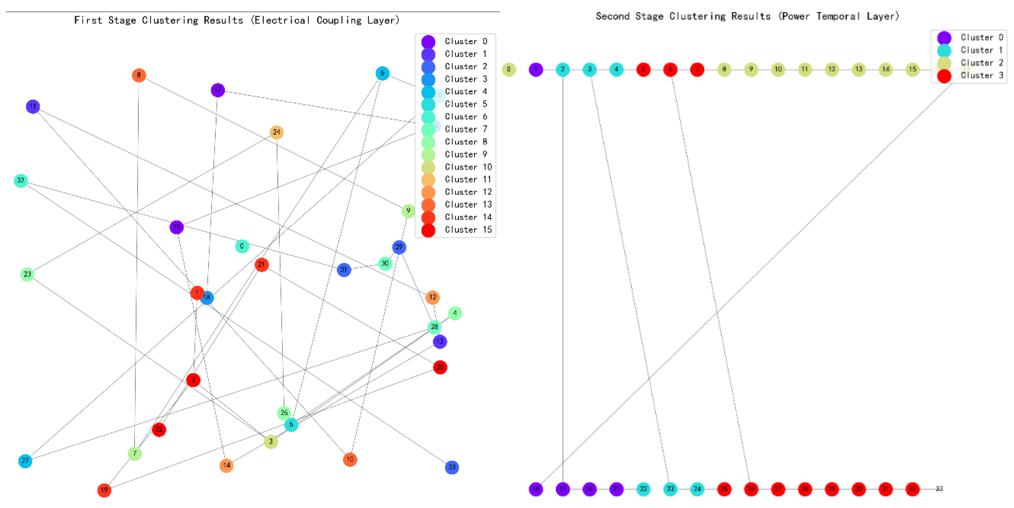
Results show that through the hierarchical feature ex-traction and hierarchical partitioning of the TC - SOM neural network, the distributed PV nodes in the IEEE 33 - bus system are finally clustered into 4 categories with significant physical meanings. Among them, the first - layer grid first achieves coarse partitioning based on geographical proximity via the Euclidean distance, and then determines the general affiliation of each node by integrating electrical coupling relationships. The second - layer grid strengthens the electrical coupling correlation using an adaptive learning rate and a Gaussian neighborhood function, and accomplishes the final partitioning of the clusters by combining power temporal features.
To verify the partitioning performance of the TC-SOM algorithm, this study, in conjunction with the research context, selects three metrics-inter-cluster tie-line power volatility, intra-cluster self-balance rate, and ramping flexibility deficit-for comparative analysis against the K-means algorithm. Specifically, a lower inter-cluster tie-line power volatility indicates more stable power exchange between clustered regions; a higher intra-cluster self-balance rate signifies a better match between power supply and load within a region; and a lower ramping flexibility deficit reflects a more abundant reserve of flexible resources inside a region. The specific data comparisons are shown in Figure 11.
From the validation result comparison chart, the two - stage SOM partitioning exhibits notable advantages across core metrics. The inter - cluster tie - line power volatility of SOM stands at 38.17, 1.8% lower than K - means’ 38.88, thus curbing fluctuations in inter - regional power exchange. The intra - cluster self - balance rate reaches 0.84, a 7.7% increase over K - means’ 0.78, strengthening the spatiotemporal matching between power supply and load within partitions. Additionally, the ramping flexibility deficit drops to 25.08, an 11.5% reduction compared to K - means’ 28.34, optimizing the aggregation efficiency of flexible resources. These three aspects synergistically provide a more characteristic - aligned optimization solution for power grid partitioning, spanning operational stability, autonomous regulation capability, and resilience enhancement.
This paper focuses on distributed photovoltaic cluster partitioning, and builds a multi-layer neural network architecture based on the adaptive SOM algorithm. By adopting an adaptive learning rate and integrating three types of indicators: scheduling distance, peak shaving capacity, and response flexibility, it achieves efficient feature extraction and accurate classification of dis-tributed photovoltaic data. The partitioning results are shown in Figure 12. Through layer-by-layer optimization processing of the three-layer SOM network, 11 photovoltaic access points in the IEEE-33 node system are divided into 4 clusters with clear physical meanings. This partitioning scheme lays the foundation for the subsequent construction of a "node demand-photovoltaic cluster-single photovoltaic" Bi-level peak shaving control model. It reduces the system's regulation dimension through clustered management, expands the channels for dynamic task logical allocation, and prepares data and architecture for the realization of hierarchical collaborative control of flexible peak shaving for distributed photovoltaics.
4.3. Flexible Peak Shaving of Distributed Photovoltaics
After completing the partitioning of distributed photovoltaic clusters, to verify the feasibility of the pro-posed collaborative peak shaving strategy for distributed photovoltaics in this paper, load disturbances are introduced into the IEEE-33 node model. These disturbances consist of one value per hour over 24 hours, which fully simulates the peak shaving scenarios when the system experiences load disturbances. The specific disturbance values are shown in Table 2.
Figure 13 shows the 24-hour output of the 11 PVs connected in the example. The distributed photovoltaics included in the system have zero output from 0-5 and 20-24 hours, while from 5-20 hours, their output increases as the light intensity rises.
Introduce the above-mentioned disturbances into the system, calculate the scheduling distance from each cluster to the disturbance node by virtue of the afore-mentioned scheduling distance index, and then allocate the peak shaving demand for each cluster according to the calculated scheduling distance. The calculation results of the scheduling distance for each cluster are shown in Table 3.
Based on the proportion of the scheduling distance from each cluster to the disturbance node, the total output required for each cluster is issued respectively. Then, each cluster controls the output of the photovoltaics it contains according to the demand. The final output results of each photovoltaic after control are shown in Figure 14.
Since the disturbance occurs in Cluster 3, the photovoltaics within this cluster operate at full output at all times, while Clusters 1, 2, and 4 adjust their output according to the peak shaving demand between 8:00 and 17:00. During peak load periods, the output of distributed photovoltaic clusters is effectively in-creased, which successfully boosts power supply and reduces the peak shaving pressure on the power grid. Compared with the period before peak shaving, the peak-valley difference of the power grid is significantly reduced, the maximum load is effectively cut down, and the minimum load has increased. When the load disturbance decreases, the required photovoltaic output is correspondingly reduced, and the output of the corresponding photovoltaic clusters decreases accordingly. The specific peak shaving curve is shown in Figure 15.
As illustrated above, photovoltaic output is intrinsically governed by solar irradiance, resulting in a daily power profile marked by pronounced peaks and troughs: steep ramps on clear-sky days, abrupt fluctuations under scattered clouds, and a complete collapse to zero at night. Pooling data across the entire 24-hour span would inject lengthy pre-sunrise and post-sunset zero-output segments-along with their low-irradiance “tails”-as a large share of invalid points. These artifacts dilute the prominence of peak-to-valley variations, inflate the mean, and suppress the variance, thereby obscuring the true variability. Accordingly, after filtering out such low-irradiance disturbances, only the effective generation window is retained for subsequent analysis to ensure both credibility and comparability of the results. To exclude the low-irradiance disturbances noted above, the analysis confines itself to the 05:00–18:00 window of reliable insolation, and the resulting peak-shaving curve is presented in Figure 16.
The figure above systematically presents the changes in four key load-balancing metrics before and after the implementation of the peak-shaving strategy. First, the load imbalance index drops sharply from its original value of 0.3443 to 0.1280, a 21.64 % improvement, demonstrating that the optimization is highly effective in peak clipping and valley filling, directly reducing the supply-demand deviation. Second, the peak-valley difference is compressed from 0.8893 to 0.6, an 11.72 % reduction, confirming that restricting the analysis to the high-irradiance window successfully mitigates intra-day power swings. Third, the standard deviation falls from 0.0975 to nearly zero, a 14.36 % decrease, indicating a markedly narrower dispersion of the power sequence and a smoother operational profile. Finally, load stability also improves by 2.55 %, further lowering the risk of frequency disturbances. Overall, the optimized peak-shaving strategy not only enhances all balancing indicators across the board but also provides a solid basis for the stable operation of power systems with high photovoltaic penetration. The specific re-duction of the peak-valley difference is shown in Figure 17.
Meanwhile, to verify the differences between traditional peak shaving methods and the Bi-level model peak shaving strategy proposed in this paper, a com-parison of their peak shaving results was conducted, with specific results shown in Figure 18. The Bi-level optimization model proposed in this paper exhibits superior smoothness in peak shaving control. By dynamically adjusting the output of distributed photovoltaics in real time, the system effectively improves the smoothness of the load after peak shaving, significantly reducing the impact caused by system load fluctuations. Moreover, the decline rate of the peak-valley difference after peak shaving with this model is higher than that of traditional peak shaving methods, resulting in better peak shaving performance.
In summary, compared with traditional peak shaving methods, the Bi-level model proposed in this paper shows obvious advantages. Based on the IEEE-33 node example, the optimized peak-valley difference is reduced by 0.074MW, with a decrease rate of 21%. It can operate more efficiently when dealing with large-scale data and complex calculations. Especially in scenarios with high-proportion photovoltaic integration, when the photovoltaic penetration rate reaches 40%, the peak shaving efficiency is 12% higher than that of traditional methods. This fully verifies the effectiveness and superiority of the Bi-level model in the collaborative regulation of large-scale distributed energy, providing a highly valuable solution for the efficient utilization and stable operation of distributed photovoltaics in future power grids.
5. Conclusions
This paper proposes a distributed photovoltaic cluster partitioning and flexible peak shaving strategy based on an improved adaptive SOM algorithm and a two-layer model, which significantly enhances the feature extraction and partitioning accuracy of distributed PV data. It effectively coordinates the output of distributed PVs both between clusters and within clusters, achieving hierarchical peak shaving control from node demand to individual PVs. The simulation results on the IEEE-33 node system strongly demonstrate the significant effects of this strategy in smoothing the load curve, reducing the peak-valley difference, and enhancing the peak shaving capability of distributed PVs, verifying the effectiveness and feasibility of the method.
(1) The improved SOM model achieves significant optimization of the network structure by incorporating a multi-layer neuron structure and an adaptive learning rate adjustment strategy into the neuron learning rule, thereby greatly enhancing the model's partitioning ability. The quantization error converges to below 0.003, effectively capturing the complex characteristics of PV output fluctuations, such as solving the problem of inaccurate division by traditional partitioning methods, and realizing the precise division of PV clusters into clusters with clear physical meanings.
(2) Compared with traditional peak shaving methods, the two-layer optimization model proposed in this paper shows significant technical advantages and engineering applicability in peak shaving control. In the case example of this paper, the load peak-valley difference can be reduced by 0.3369 MW, with a reduction rate of 13.62%. Under the high proportion access scenario with a PV penetration rate of 33%, the peak shaving efficiency is 12% higher than that of traditional methods, which significantly smooths the load curve and fully exploits the peak shaving potential of dis-tributed PVs.
(3) The strategy proposed in this paper provides an effective solution for the precise control of distributed PV clusters. It reduces the system control dimension through cluster management, has higher efficiency when dealing with large-scale data, and has a smoother load curve after peak shaving than traditional methods. It provides technical support for the efficient and stable operation of the power grid with a high proportion of PV access and has good engineering application value.
Author Contributions
T.Z.: supervision, conceptualization, methodology, writing-review & editing, funding acquisition. Y.M.: investigation, data curation, formal analysis, writing-original draft, visualization. Z.H.: investigation, validation, data curation, writing-review & editing. C. W.: supervision, methodology, resources, writing-review & editing. All authors have read and agreed to the published version of the manuscript.
Funding
This research was funded by the Natural Science Foundation of Jiangsu Province (No. BK20241481) and the Fundamental Research Funds for the Central Universities (No. 30922010709).
Data Availability Statement
The original contributions presented in this study are included in the article. Further inquiries can be directed to the corresponding authors.
Conflicts of Interest
The authors declare no conflicts of interest.
References
- Xia, Y.; Xu, Y.; Wang, Y.; Li, Z. Power system stability with a high penetration of inverter-based re-sources. IEEE Proc. 2023, 111, 5036–5049. [Google Scholar] [CrossRef]
- Yu, D.; Sun, D.; Xu, D.; Liu, J. Challenges, solutions and prospects for power-energy balance in new-type power systems. Proc. CSEE 2025, 45, 2039–2057. [Google Scholar] [CrossRef]
- Xia, Y.; Zhang, H.; Wang, Y. Voltage stability analysis of power systems with high shares of renewable energy. IEEE Proc. 2023, 111, 5050–5062. [Google Scholar] [CrossRef]
- Xiao, Y.; Wang, X.; Wang, X. A review of electricity market research for high-penetration renewable energy. Proc. CSEE 2018, 38, 663–674. [Google Scholar] [CrossRef]
- Liu, Z.; Guo, G.; Gong, D.; Xuan, L.; He, F.; Wan, X.; Zhou, D. Cluster Partitioning Method for High-PV-Penetration Distribution Network Based on mGA-PSO Algorithm. Energies 2025, 18, 1197. [Google Scholar] [CrossRef]
- Zhang, L.; Wang, Y.; Li, H.; Chen, Z. Flexible active power control of distributed photovoltaic systems with integrated battery using series converter configurations. IEEE J. Emerg. Sel. Topics Power Electron. 2022, 10, 6891–6909. [Google Scholar] [CrossRef]
- Int. Energy Agency (IEA). Renewable energy integration in power systems: Global best practices. IEA: Paris, France, 2024; Rep. IEA-REPORT-2024. [Google Scholar]
- Zhao, P.; Liu, X.; Qu, H.; Liu, N.; Zhang, Y.; Xiao, C. Multi-Objective Cooperative Optimization Model for Source–Grid–Storage in Distribution Networks for Enhanced PV Absorption. Processes 2025, 13, 2841. [Google Scholar] [CrossRef]
- Wang, Y.; Zhang, N.; Kang, C.; Li, X. Two-level distributed Volt/Var control using aggregated PV inverters in distribution networks. IEEE Trans. Power Del. 2021, 35, 1844–1855. [Google Scholar] [CrossRef]
- Ye, Z.; Li, X.; Jiang, F.; Liu, X. Hierarchical optimal economic dispatch of wind-solar-thermal-storage hybrid system considering optimal energy curtailment rate. Power Syst. Technol. 2021, 45, 2270–2280. [Google Scholar] [CrossRef]
- Zhou, T.; He, W.; Li, H.; Zhang, Y. A review of energy storage auxiliary operation and optimal configuration under new power systems. J. Nanjing Univ. Inf. Sci. Technol. (Nat. Sci. Ed.) 2025. early access. [Google Scholar] [CrossRef]
- Chai, Y.; Li, W.; Tang, Y. Network partition and voltage coordination control for distribution networks with high penetration of distributed PV units. IEEE Trans. Power Syst. 2018, 33, 3396–3407. [Google Scholar] [CrossRef]
- National Energy Administration (NEA). Measures for the Administration of the Development and Construction of Distributed Photovoltaic Power Generation (No. 7〔2025〕). [Government Gazette of the State Council 2025]. 2025. Available online: http://www.gov.cn/gongbao/2025/issue_11946/202503/content_7015853.html.
- Yan, H.D.; Liu, W.; Li, C. Dynamic peak-shaving strategy for high-penetration PV systems considering load uncertainty. Front. Energy Res. 2022, 10, 900825. [Google Scholar] [CrossRef]
- Bu, Q.; Lu, P.; Li, W.; Chen, J. Intelligent partitioning strategy of distributed photovoltaic clusters in distribution networks based on SLM-RBF. J. Shanghai Jiao Tong Univ. (Engl. Ed.) 2024, 29, 153–162. [Google Scholar] [CrossRef]
- Chen, L.; Huang, X.; Zhang, G.; Liu, J. Adaptive dynamic droop control for photovoltaic-rich distribution networks considering photovoltaic uncertainties. IET Renew. Power Gener. 2023, 17, 2035–2046. [Google Scholar] [CrossRef]
- Li, X.; Ye, Z.; Jiang, F.; Liu, X. Cooperative model predictive control for distributed photovoltaic power generation systems. IEEE Access 2021, 9, 135622–135633. [Google Scholar] [CrossRef]
- Bidram, A.; Davoudi, A.; Lewis, F.L.; Guerrero, J.M. Distributed cooperative control of microgrids using a communication network. IEEE Trans. Power Syst. 2017, 32, 3469–3483. [Google Scholar] [CrossRef]
- Wang, Y.; Zhang, N.; Kang, C.; Li, X. A distributed control strategy for voltage regulation in active distribution networks with high-penetration PV systems. IEEE Trans. Smart Grid 2021, 12, 2349–2361. [Google Scholar] [CrossRef]
- Han, X.Q.; Liu, W.Y.; Pang, Q.L.; Zhang, X.Y. A control model for electric power load participating in system peak-shaving considering day-ahead spot market risks. Power Syst. Prot. Control 2022, 50, 55–67. [Google Scholar] [CrossRef]
- Furao, S.; Ogura, T.; Hasegawa, O. An enhanced self-organizing incremental neural network for online unsupervised learning. Neural Netw. 2007, 20, 996–1009. [Google Scholar] [CrossRef]
- Pöllä, D.; Kohonen, T.; Parviainen, J. Deep self-organizing maps for unsupervised image classification. Int. J. Neural Syst. 2019, 29, 1950009. [Google Scholar] [CrossRef]
- Baran, M.E.; Wu, F.F. Optimal placement of capacitors in radial distribution systems. IEEE Trans. Power Del. 1989, 4, 725–734. [Google Scholar] [CrossRef]
Figure 1.
Framework of this paper.
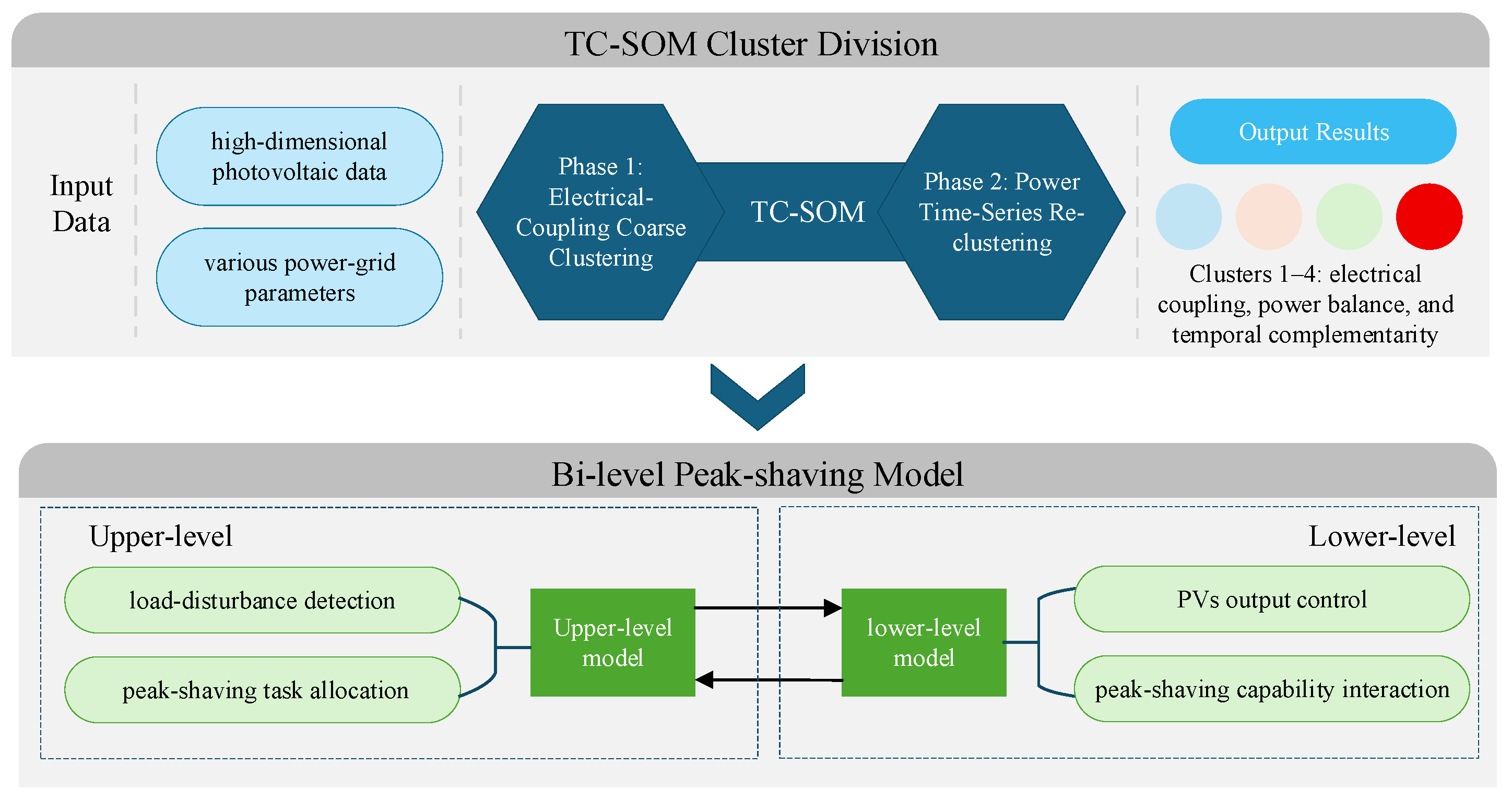
Figure 2.
Topological structure of single-layer SOM
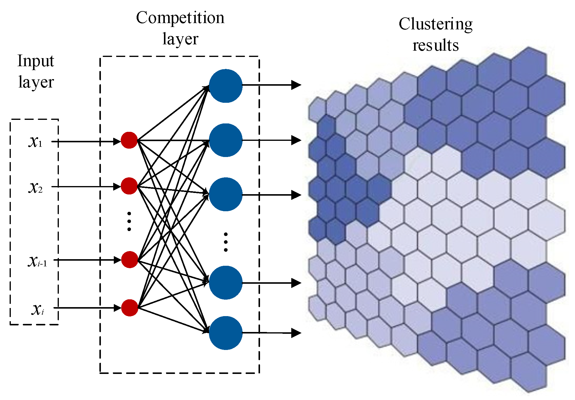
Figure 3.
TC-SOM topology map
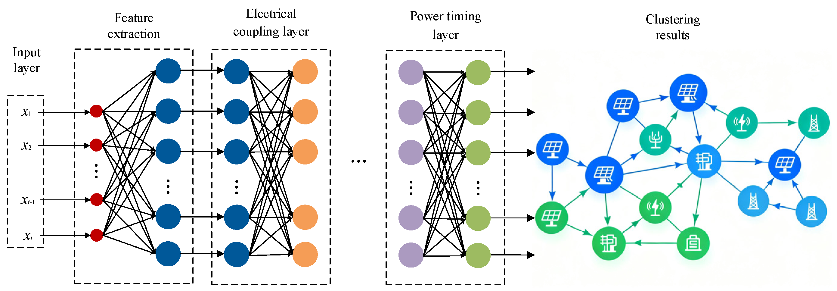
Figure 4.
Flowchart of distributed photovoltaic cluster partitioning based on TC-SOM
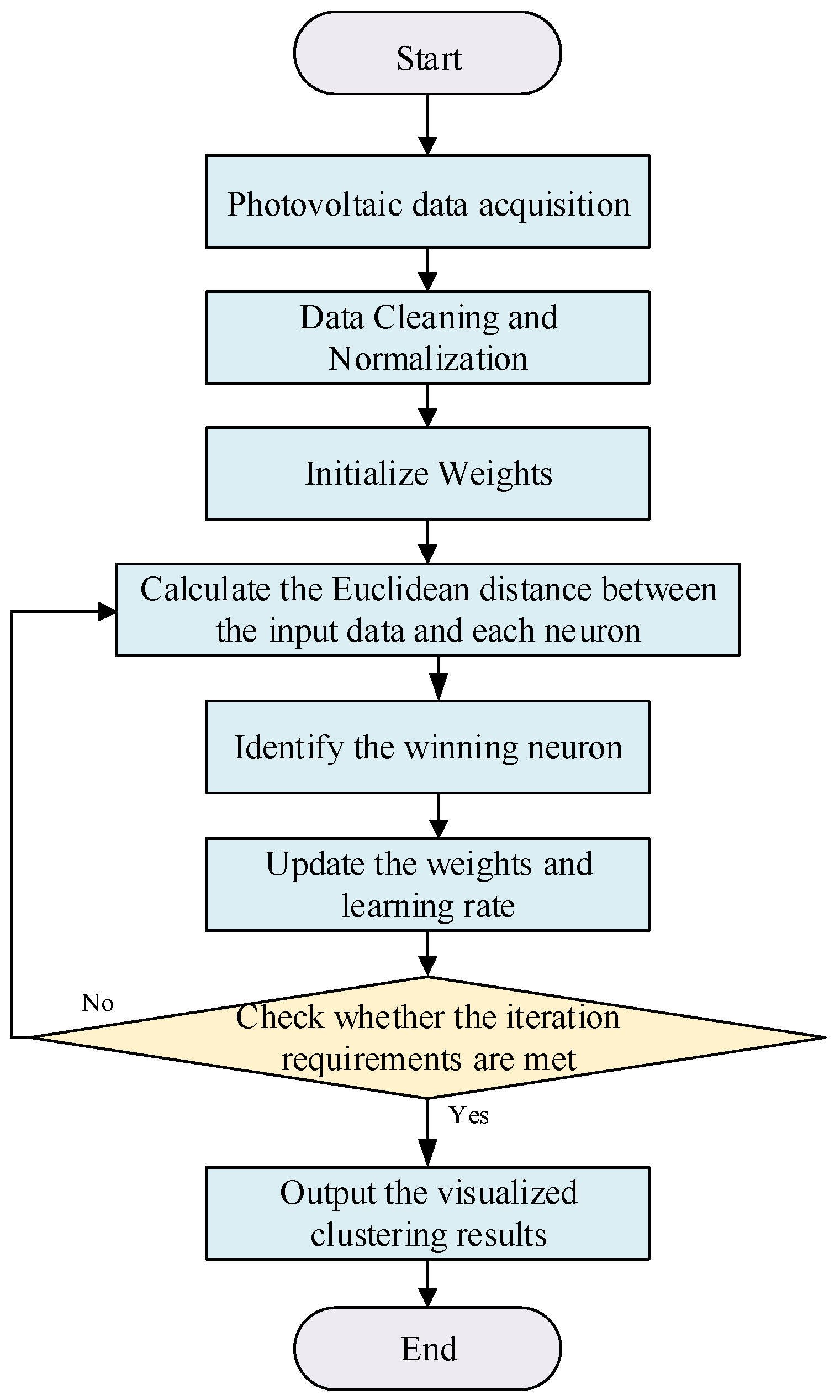
Figure 5.
Bi-level model architecture for flexible peak shaving of distributed PV
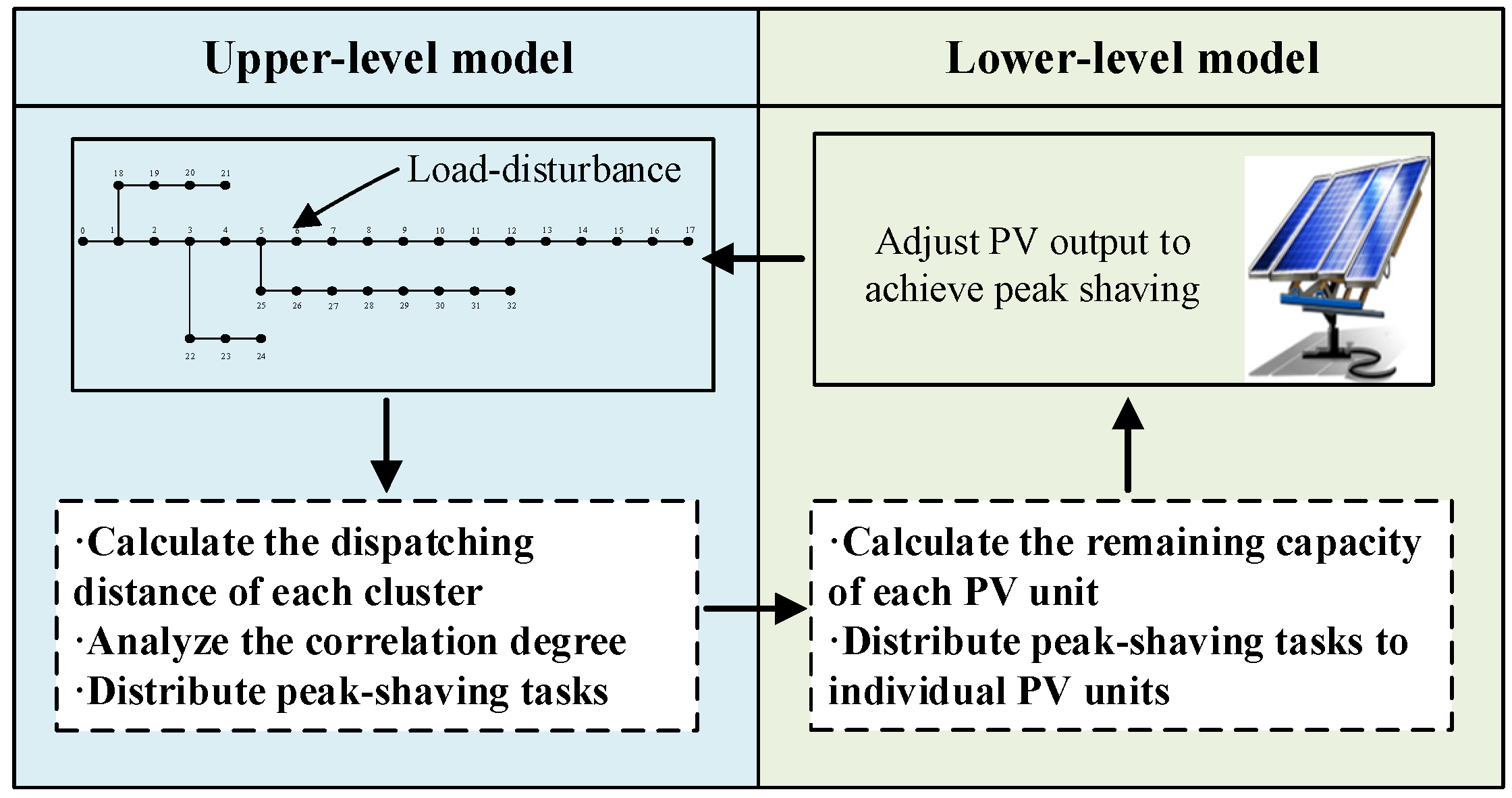
Figure 6.
Structure of upper-level model
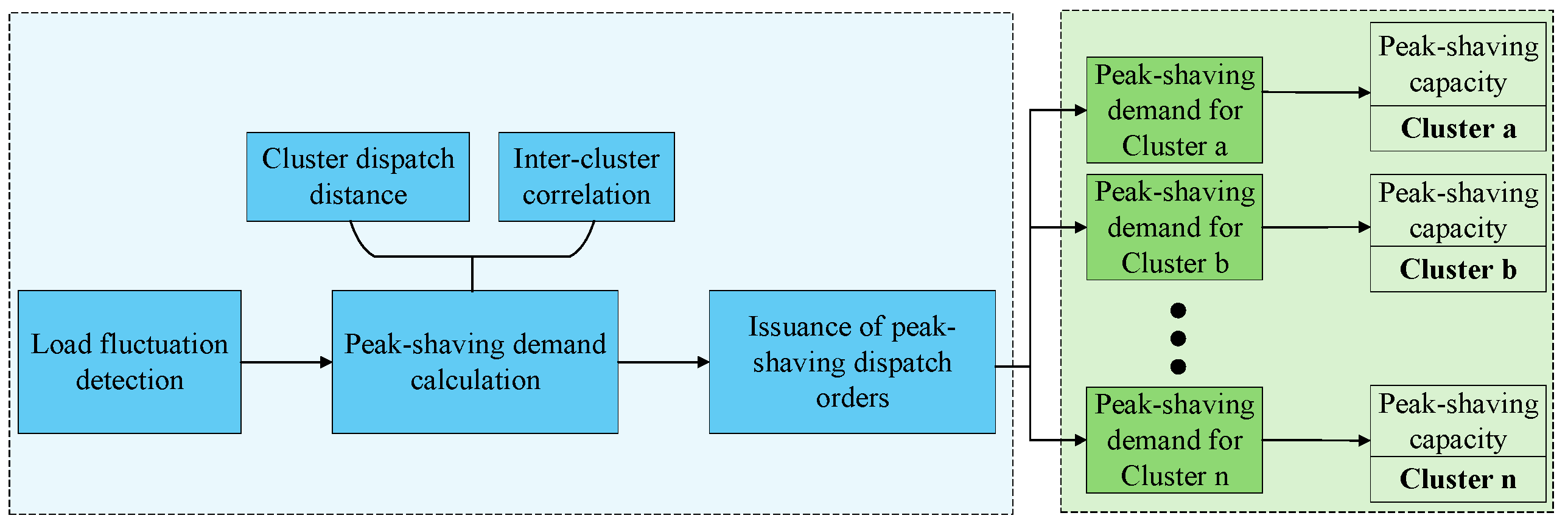
Figure 7.
Control process of distributed PV in lower layer
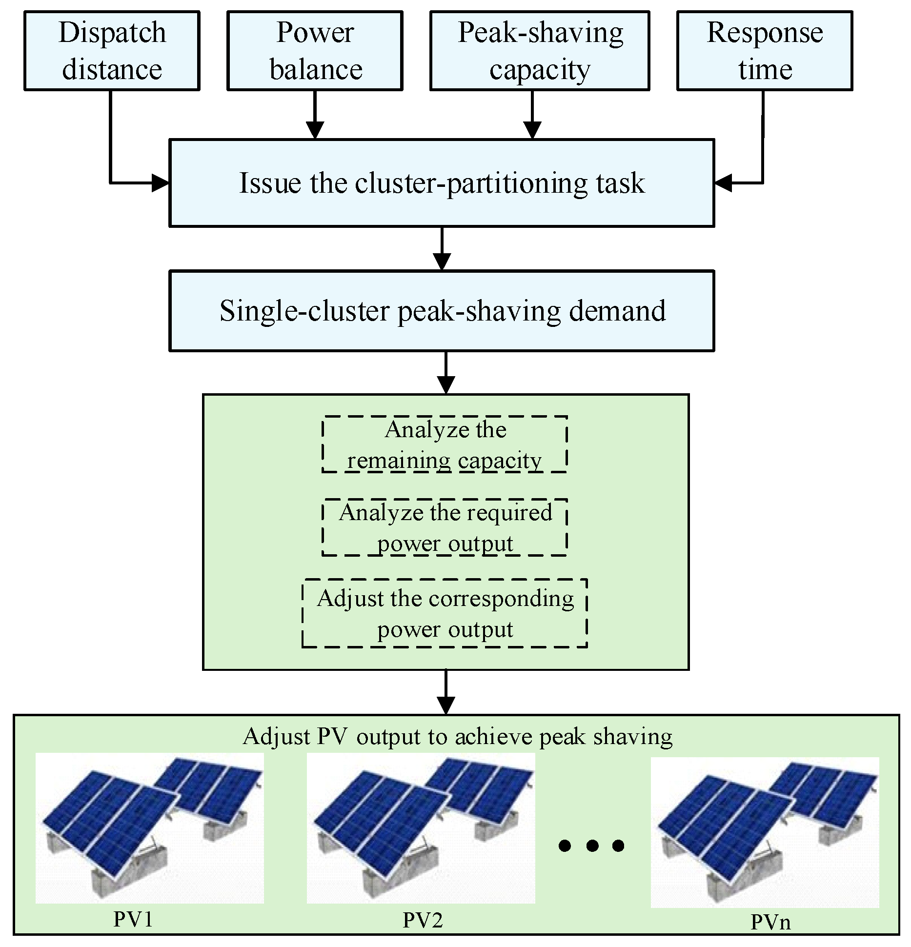
Figure 9.
Diagram of IEEE 33-node system
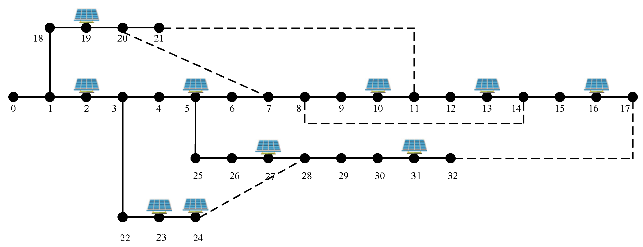
Figure 11.
Algorithm performance comparison
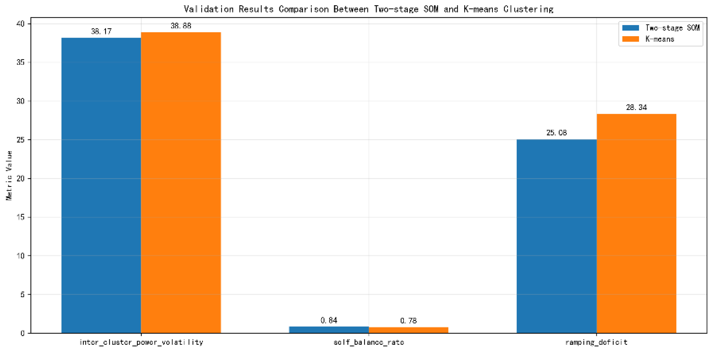
Figure 12.
Partitioning results of distributed PV clusters
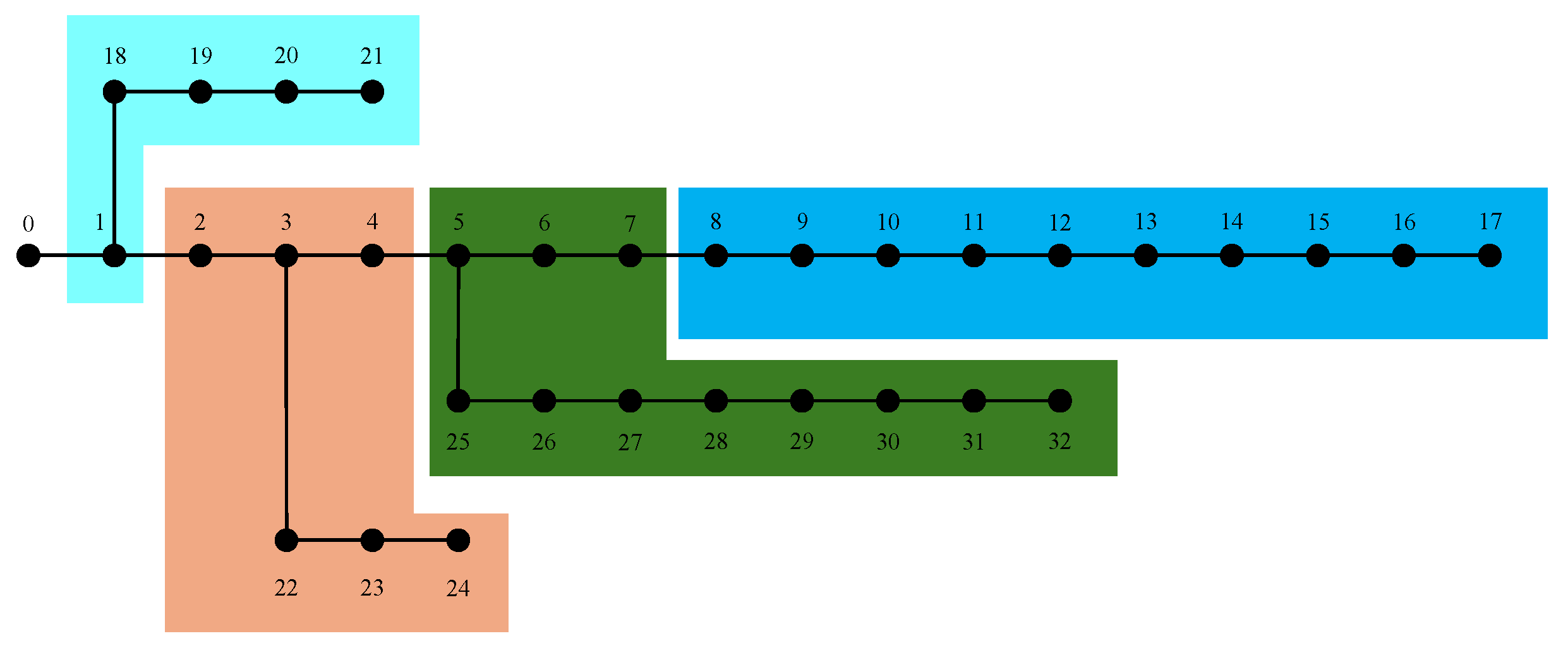
Figure 13.
24-hour power output curve of PV system
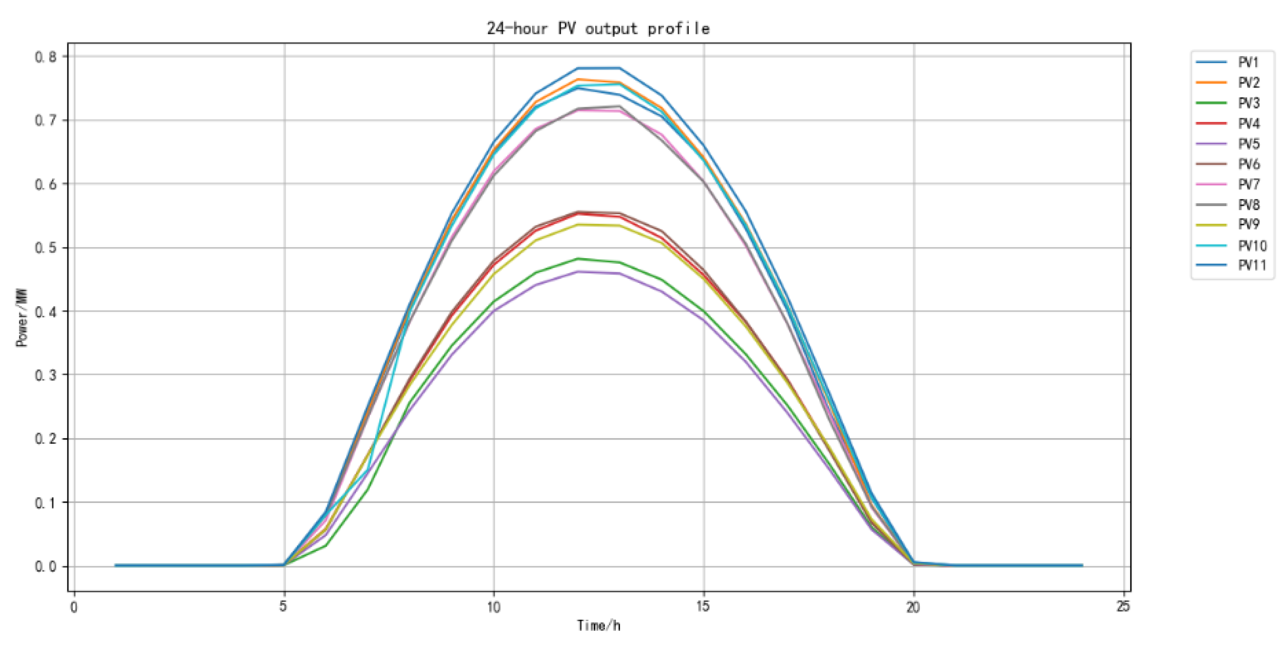
Figure 14.
PV output curve within 24 hours after regulation
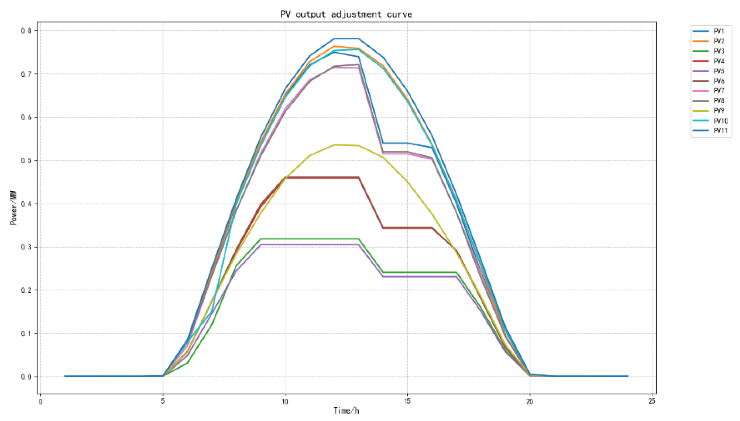
Figure 15.
Comparison of the PV regulation curve after control and the original load curve
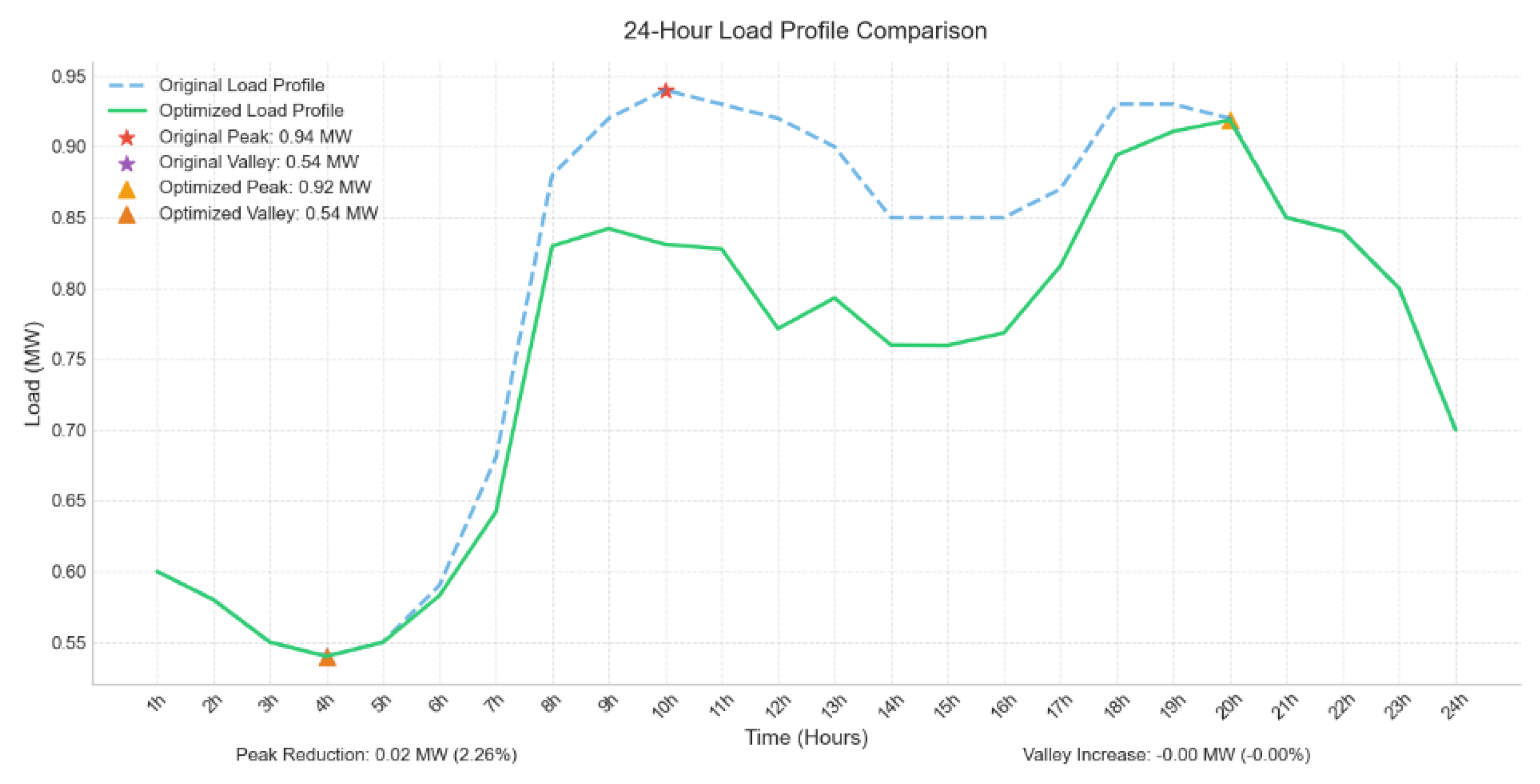
Figure 16.
Peak-shaving curve comparison for the 05:00–18:00 window
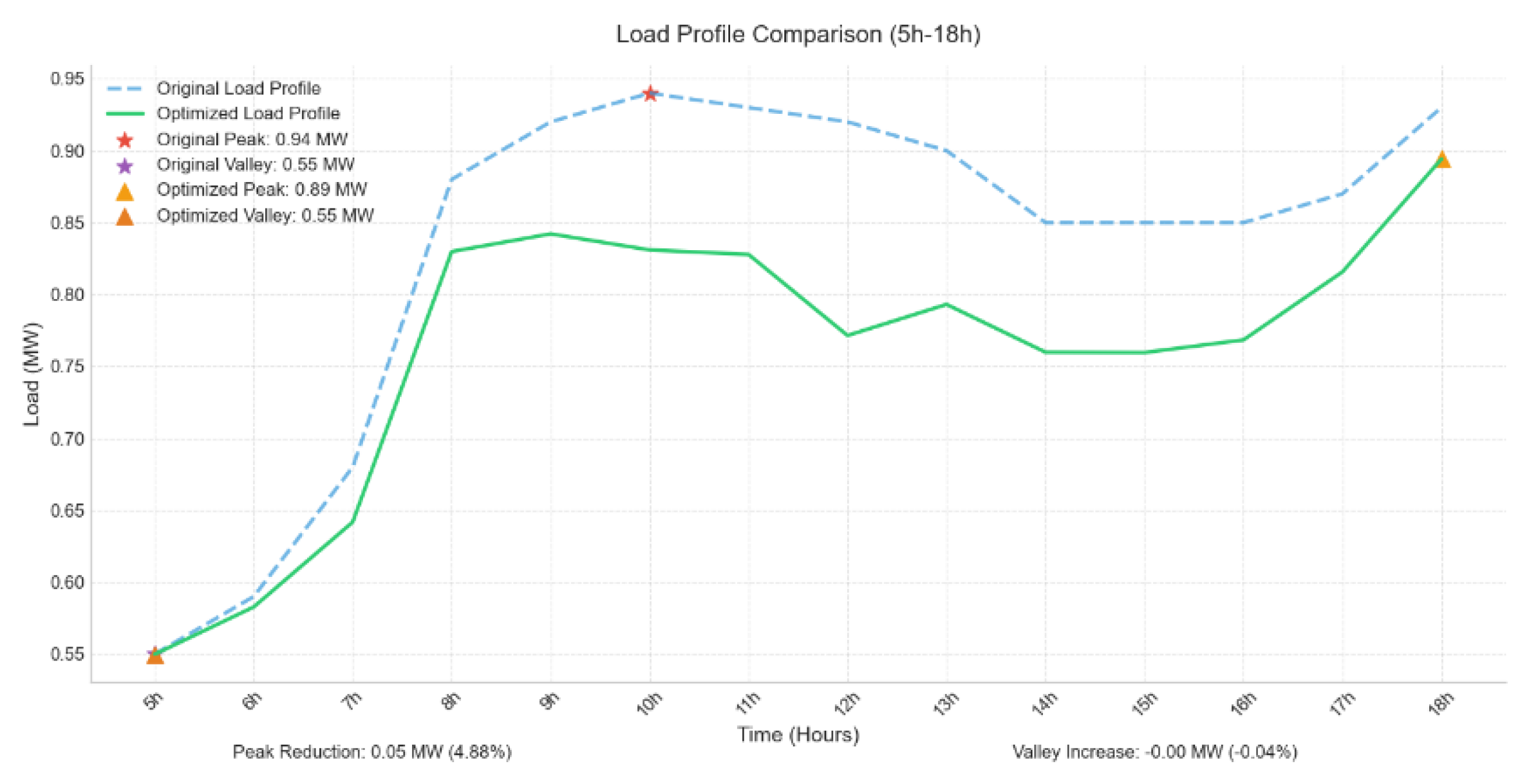
Figure 17.
Comparison of peak-shaving indicators after regulation
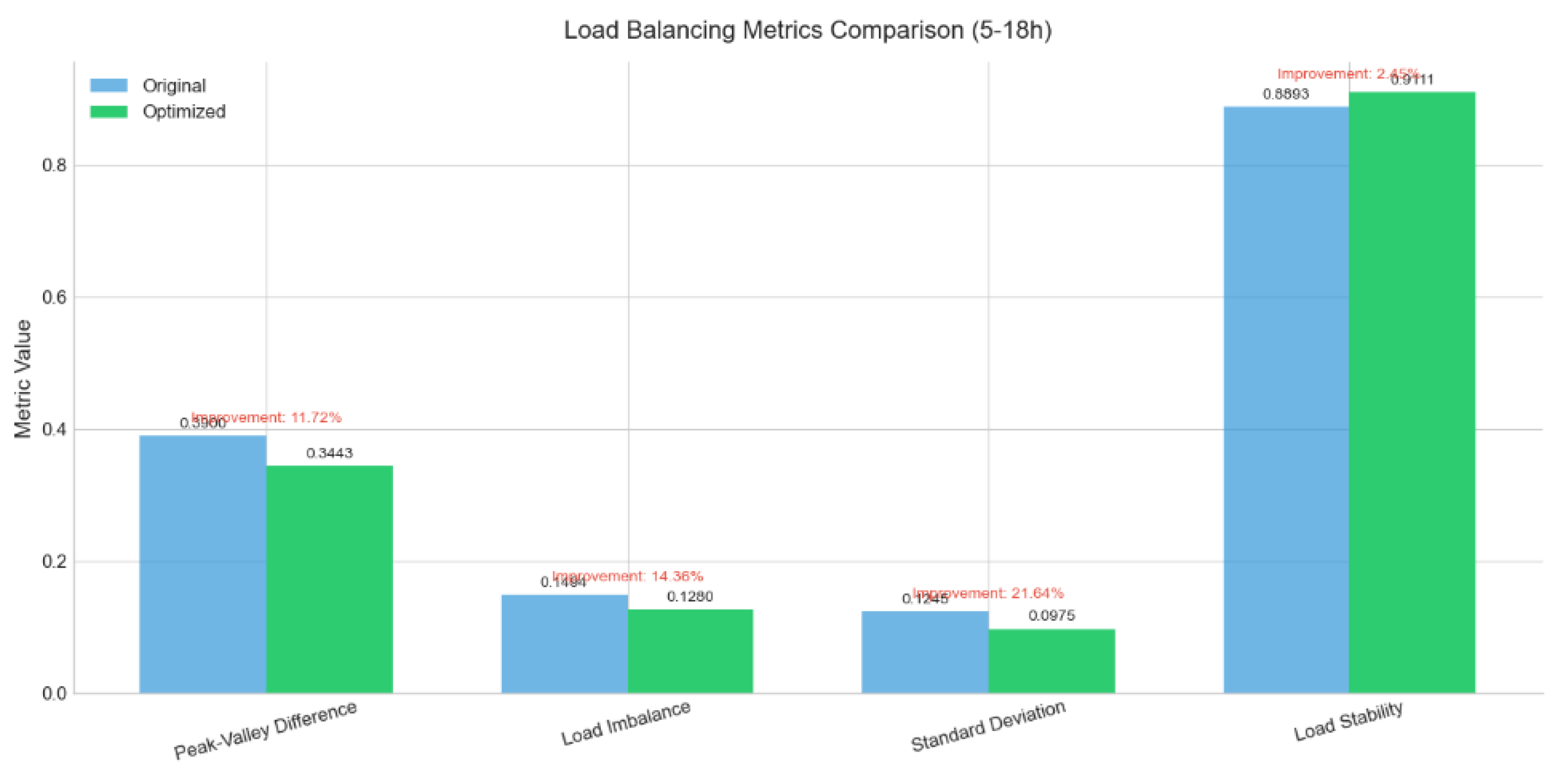
Figure 18.
Comparison between traditional peak-shaving methods and the methods in this paper
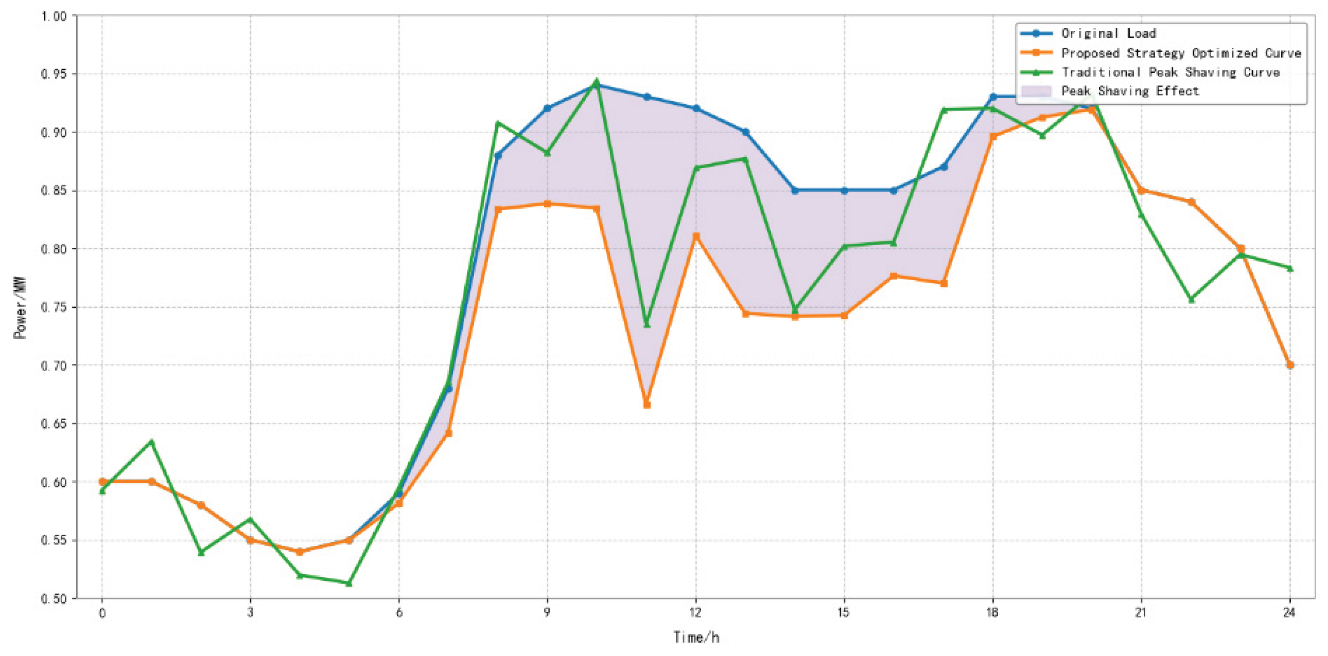

Table 1.
Node numbers for PV integrations.
| PV | Nodes | PV | Nodes |
|---|---|---|---|
| PV1 | 2 | PV7 | 23 |
| PV2 | 5 | PV8 | 24 |
| PV3 | 10 | PV9 | 26 |
| PV4 | 13 | PV10 | 27 |
| PV5 | 16 | PV11 | 31 |
| PV6 | 19 |
Table 2.
24-Hour values of load disturbances
| Time | Load(p.u.) | Time | Load(p.u.) |
|---|---|---|---|
| 1 | 0.6 | 13 | 0.9 |
| 2 | 0.58 | 14 | 0.85 |
| 3 | 0.55 | 15 | 0.85 |
| 4 | 0.54 | 16 | 0.85 |
| 5 | 0.55 | 17 | 0.87 |
| 6 | 0.59 | 18 | 0.93 |
| 7 | 0.68 | 19 | 0.93 |
| 8 | 0.88 | 20 | 0.92 |
| 9 | 0.92 | 21 | 0.85 |
| 10 | 0.94 | 22 | 0.84 |
| 11 | 0.93 | 23 | 0.8 |
| 12 | 0.92 | 24 | 0.7 |
Table 3.
Scheduling distance from each cluster to disturbance node
| Clusters | Central Nodes | Scheduling Distance |
|---|---|---|
| 1 | 19 | 0.426 |
| 2 | 23 | 0.311 |
| 3 | 29 | 0 |
Disclaimer/Publisher’s Note: The statements, opinions and data contained in all publications are solely those of the individual author(s) and contributor(s) and not of MDPI and/or the editor(s). MDPI and/or the editor(s) disclaim responsibility for any injury to people or property resulting from any ideas, methods, instructions or products referred to in the content. |
© 2025 by the authors. Licensee MDPI, Basel, Switzerland. This article is an open access article distributed under the terms and conditions of the Creative Commons Attribution (CC BY) license (http://creativecommons.org/licenses/by/4.0/).
Copyright: This open access article is published under a Creative Commons CC BY 4.0 license, which permit the free download, distribution, and reuse, provided that the author and preprint are cited in any reuse.


