
Submitted:
25 October 2025
Posted:
27 October 2025
You are already at the latest version
Abstract
A Plithogenic Set extends the classical fuzzy, intuitionistic, and neutrosophic paradigms by assigning attribute-based membership and contradiction values to elements, and the same ideas naturally extend to graph-based structures such as the Plithogenic Graph. Neutrosophic sets, in turn, represent elements with independent degrees of truth, indeterminacy, and falsity on the unit interval, thus handling incomplete, inconsistent, and ambiguous information effectively. This paper investigates the Plithogenic Graph, the Plithogenic Vertex Graph, and the Plithogenic Edge Graph. In addition, it examines the Intuitionistic Fuzzy Vertex Graph and Edge Graph, the Neutrosophic Vertex HyperGraph and Neutrosophic Edge HyperGraph, and the Neutrosophic Vertex SuperHyperGraph and Neutrosophic Edge SuperHyperGraph.
Keywords:
plithogenic set
; plithogenic graph
; neutrosophic graph
; neutrosophic set
1. Preliminaries
This section presents the fundamental concepts and definitions that underpin the discussions in this paper. Throughout this paper, all structures and sets are assumed to be finite. Moreover, the graph is assumed to be undirected and simple.
1.1. Intuitionistic Fuzzy Graph
An intuitionistic fuzzy graph assigns to each vertex and edge a pair of degrees (membership and nonmembership), together with a hesitation margin, allowing one to model relational uncertainty more expressively [1,2,3,4,5]. It is well known that this framework generalizes the classical fuzzy graph [6,7].
Definition 1
(Intuitionistic Fuzzy Graph). [8] Let be a finite, simple, undirected (crisp) graph with . An intuitionistic fuzzy graph (IFG) on G is a pair
where
- assigns to each vertex two numbers (membership and nonmembership) with
- assigns to each edge two numbers with
These assignments satisfy the standard consistency (compatibility) constraints for every :
Example 1 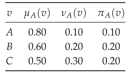
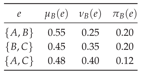
(Real-world IFG: Supply–chain collaboration network). Three regional warehouses consider joint replenishment. An undirected edge indicates that the pair can collaborate (e.g., share transportation or inventory). Uncertainty comes from fluctuating demand, carrier reliability, and contractual constraints.
Graph.Let
Vertex grades.Interpret as the readiness of warehouse v to collaborate (higher is better) and as the incompatibility of v with collaboration (higher is worse). Hesitation is .
Edge grades.Interpret as the pairwise feasibility of a joint plan between u and v, and as the pairwise opposition (e.g., contractual or capacity frictions). Hesitation is . Choose
Consistency (IFG constraints).For every we verify
Indeed:
and for each edge.
Warehouse pairs with higher readiness and lower incompatibility (e.g., ) exhibit larger and smaller , signaling easier collaboration. Pairs facing capacity mismatches or policy frictions (e.g., ) show larger and smaller . The hesitation terms capture unknowns such as seasonal spikes or carrier volatility. Thus is a favorable link, is moderate, and is the riskiest partnership under current information. This constitutes an intuitionistic fuzzy graph model of a supply–chain collaboration network.
1.2. Neutrosophic Set and Graph
Neutrosophic sets model elements via independent truth, indeterminacy, and falsity degrees in , accommodating incomplete, inconsistent, and ambiguous information effectively [9,10,11,12]. A Neutrosophic Set generalizes the notions of Fuzzy Sets [13,14,15] and Intuitionistic Fuzzy Sets [16,17].
Neutrosophic graphs represent vertices and edges with truth, indeterminacy, and falsity memberships, enabling uncertain, contradictory, or incomplete modeling in networks [18,19,20,21,22]. Related notions include the Quadripartitioned Neutrosophic Graph [23,24,25], the Pentapartitioned Neutrosophic Graph [26,27,28,29], the Bipolar Neutrosophic Graph [30,31,32], and the Neutrosophic Directed Graph [33,34,35], among others.
Definition 2 (Neutrosophic Graph (single–valued)). [22] Let V be a finite vertex set and an undirected edge set. A (single–valued) neutrosophic graph on is a pair
where
- assigns to each its truth-, indeterminacy-, and falsity-memberships with
- assigns to each its truth-, indeterminacy-, and falsity-memberships with
and the vertex–edge compatibility constraints hold for every edge :
A neutrosophic vertex graph assigns to each vertex degrees of truth, indeterminacy, and falsity, thereby inducing compatible edge evaluations to effectively represent uncertainty [36]. A neutrosophic edge graph assigns truth, indeterminacy, and falsity degrees directly to each edge, with corresponding constraints on vertices to capture relational uncertainty. These structures are known to generalize fuzzy vertex [37,38]/edge graphs [39,40].
Definition 3
(Neutrosophic Vertex Graph). [36] Let V be a finite vertex set and be (crisp) edges. A neutrosophic vertex graph on consists of vertex assignments
When one wishes to induce edge grades from the vertex information, the canonical edge relation on E is defined by
This choice is consistent with the vertex–edge bounds in the neutrosophic graph definition above.
Definition 4
(Neutrosophic Edge Graph). Let V be a finite vertex set and be (crisp) edges. A neutrosophic edge graph on assigns to each edge the triple
If vertex grades are also specified, they must be compatible with the edges in the sense that, for every ,
1.3. Plithogenic Set and Graph
A Plithogenic Set [41,42,43,44,45] models elements with attribute-based membership and contradiction functions, extending fuzzy [14,46], intuitionistic [16,47,48,49], and neutrosophic sets [9,50]. A plithogenic graph assigns attribute-based membership vectors and contradiction functions to vertices or edges, generalizing fuzzy, intuitionistic, and neutrosophic models [51,52,53,54].
Definition 5
(Plithogenic Set). [41,55] Let S be a universal set and a nonempty subset. A Plithogenic Set is a quintuple
where
- v is an attribute,
- is the set of possible values of the attribute v,
- is theDegree of Appurtenance Function (DAF),1
- is theDegree of Contradiction Function (DCF).
The DCF satisfies, for all ,
Here is the appurtenance dimension and the contradiction dimension.
Definition 6
(Plithogenic Graph). (cf. [53,57]) Let be a crisp (simple, undirected) graph with . A plithogenic graph is a pair
where the vertex and edge components are specified as follows.
Vertex component.
with
- a chosen vertex subset;
- ℓ an attribute attached to vertices;
- the set of possible values of ℓ;
- the vertex DAF;
- the vertex DCF.
Edge component.
with
- a chosen edge subset;
- m an attribute attached to edges;
- the set of possible values of m;
- the edge DAF;
- the edge DCF.
All inequalities in are interpreted componentwise. Fix . The following axioms are required.
- (A1)
- Edge–vertex compatibility (appurtenance bound).For all and ,
- (A2)
- Contradiction consistency (edge vs. vertices).For all ,
- (A3)
- Reflexivity and symmetry of DCF.
1.4. Hypergraphs and Superhypergraphs
A hypergraph extends an ordinary graph by permitting each edge to join an arbitrary nonempty subset of vertices; this allows multiway (higher-order) relationships to be modeled within a single framework [6,58,59,60,61]. A SuperHyperGraph captures hierarchical interaction patterns by iterating the powerset construction to a prescribed depth n, thereby organizing vertices and edges across multiple levels [45,62,63,64,65,66,67].
Definition 7
(Base set). A base set (or ground set) is a fixed finite set S from which all subsequent objects are formed:
All constructions below ultimately draw their elements from S.
Definition 9
Example 2
(Hypergraph: Project Teams and Tasks). Consider a company with employees . Each task may require any number of employees. Model the assignment by the hypergraph
Here, each hyperedge is the (nonempty) set of employees assigned to task i: task 1 needs , task 2 needs , and task 3 needs . Because hyperedges may contain more than two vertices, this representation naturally captures multi-person collaborations that a simple graph (pairwise edges only) cannot express.
Definition 10
When excluding the empty set, write
Example 3
(n-th powerset: Meal Planning from Ingredients). Let the ingredient set be . The first powerset is
whose elements can be interpreted asrecipes (ingredient bundles). The second powerset
consists of all menus (collections of recipes), e.g.
If one excludes the empty set, then , and similarly . This hierarchy reflects real planning: level 1 groups ingredients into recipes, while level 2 groups recipes into menus (e.g., for a day or event).
Definition 11
(n-SuperHyperGraph). [45,75,76,77] Fix a finite base set and . Define and for . Ann -SuperHyperGraph is a pair
whose elements of V are the n-supervertices and whose members of E are nonempty sets of supervertices (the n-superedges).
whose elements of V are the n-supervertices and whose members of E are nonempty sets of supervertices (the n-superedges).
whose elements of V are the n-supervertices and whose members of E are nonempty sets of supervertices (the n-superedges).
Example 4
(n-SuperHyperGraph: Consortia of Project Teams ()). Let the base set of individual researchers be . Then is the set of all teams, and is the set of consortia of teams. Define the supervertex set
and superedges (joint milestones that require multiple consortia)
The pair is a 2-SuperHyperGraph: elements of V are supervertices (consortia of teams), and each is a nonempty set of such supervertices (asuperedge) that must coordinate to deliver a milestone. This models hierarchical collaboration: individuals → teams → consortia, with superedges capturing multi-consortia interactions typical in large research programs.
1.5. Neutrosophic n-Superhypergraph
A single-valued neutrosophic hypergraph is a hypergraph constructed from a single-valued neutrosophic graph [11,78,79,80,81,82], and a single-valued neutrosophic superhypergraph is a superhypergraph constructed from a single-valued neutrosophic graph. A single-valued neutrosophic hypergraph and a neutrosophic n-superhypergraph are given as follows [45,83].
Definition 12
(Single-Valued Neutrosophic Hypergraph). (cf. [79,84,85,86,87]) Let be a finite vertex set and let be a family of nontrivial single-valued neutrosophic subsets of V such that
Each neutrosophic hyperedge is given by
where
Then is called asingle-valued neutrosophic hypergraph.
Example 5
(Single-Valued Neutrosophic Hypergraph). Let and let , where each is a single-valued neutrosophic subset of V. Define, for every , the triples with component sum :
Then , so the coverage condition holds. Thus is a single-valued neutrosophic hypergraph. (One may interpret as two “tasks” with graded truth/indeterminacy/falsity of each vertex’s involvement.)
Definition 13
Ann-Superhypergraph is a pair with
ANeutrosophic n-Superhypergraph on is a tuple
where
- assign to each n-supervertex its truth, indeterminacy, and falsity degrees, with
-
encode a neutrosophic incidence (membership) of v into a superedge , subject tothe vertex–domination (componentwise) constraintsand the support condition
Thus describe the intrinsic neutrosophic status of supervertices, while specify how those supervertices contribute neutrosophically to each superedge.
Example 6
(Neutrosophic 2-Superhypergraph). Let the base set be . Then and . Choose the supervertex set
and superedges
Assign neutrosophic vertex degrees (each component in , sums ):
Define edge incidences only on vertices that belong to each superedge (support condition), and make them componentwise dominated by the corresponding vertex degrees:
For any and , set . By construction,
and each incidence triple sums to . Therefore is a neutrosophic 2-superhypergraph. (One may view as single/team units, and as coalitions with graded participation.)
2. Review and Main Results
We now present the results established in this paper.
2.1. Intuitionistic Fuzzy Vertex Graph
An intuitionistic fuzzy vertex graph assigns to each vertex membership and nonmembership degrees with hesitation, inducing compatible edge assessments automatically.
Definition 14
(Intuitionistic Fuzzy Vertex Graph). Let be as above. Anintuitionistic fuzzy vertex graph (IFVG) on G specifies only vertex grades
with hesitation .
When one wishes to derive edge grades from the vertex information, thecanonical induced edge assignment on E is defined by
which automatically satisfies and the IFG compatibility inequalities.
Example 7 (Intuitionistic Fuzzy Vertex Graph(IFVG)). Let with and . Assign vertex grades
so for all . The canonical induced edge grades are
Hence
and in each case . Thus defines an IFVG on G.
2.2. Intuitionistic Fuzzy Edge Graph
An intuitionistic fuzzy edge graph labels every edge with membership and nonmembership degrees under hesitation, constraining vertex grades for consistency.
Definition 15
(Intuitionistic Fuzzy Edge Graph). Let be as above. Anintuitionistic fuzzy edge graph (IFEG) on G specifies only edge grades
with hesitation .
If vertex grades are also provided, then must satisfy, for all ,
Example 8 (Intuitionistic Fuzzy Edge Graph(IFEG)). Let with and . Specify edge grades
so for all . Provide vertex grades
each satisfying . Then the IF edge–vertex compatibility holds:
Hence defines a consistent IFEG on G.
2.3. Plithogenic Vertex Graph
A plithogenic vertex graph attaches attribute based memberships to vertices with contradiction function, generating edge memberships via signed aggregation rules.
Definition 16 (Plithogenic Vertex Graph (PVG)). Let be a finite simple undirected graph. Fix
- an attribute alphabet for vertices;
- a sign map indicating, for each attribute value , whether higher membership is favorable or unfavorable;
-
a degree of appurtenance function (DAF)assigning to each vertex and attribute value an s-tuple of membership degrees (componentwise order on );
-
a degree of contradiction function (DCF)with and (componentwise).
The canonical induced edge DAF is the map
where act componentwise on . The structure
is called aPlithogenic Vertex Graph (PVG). (Other t-norm / t-conorm pairs may replace ; we fix these to connect with neutrosophic graphs.)
Example 9 (Plithogenic Vertex Graph PVG): Team formation). Let with and . Take a vertex attribute alphabet
Work with . Set a symmetric vertex DCF , . Give vertex DAF values (componentwise scalars in ):
The canonical induced edge DAF is
Hence
Thus is a PVG that aggregates vertex “reliability” and “risk” into edge memberships via the signed rule.
Theorem 1
(PVG generalizes the Neutrosophic Vertex Graph). Every single-valued Neutrosophic Vertex Graph (with canonical induced edges , , ) is a special case of a PVG.
Proof.
Given and , define a PVG by
take , set the vertex DAF
and choose any symmetric DCF with (its values are immaterial for this embedding). By the PVG definition,
Thus the PVG reproduces exactly the neutrosophic vertex graph (both vertex and canonically induced edge degrees), proving that NVGs are PVGs with the above specialization. □
2.4. Plithogenic Edge Graph
A plithogenic edge graph assigns attribute based memberships to edges with contradiction function, optionally bounded by vertex memberships for coherence.
Definition 17 (Plithogenic Edge Graph (PEG)). Let be a finite simple undirected graph. Fix
- an attribute alphabet for edges;
- a sign map;
- an edge DAF
-
an edge DCFwith and (componentwise).
Optionally, if vertex degrees are given on the same alphabet, we require the compatibility bounds for every and :
all componentwise in . The structure
is called a Plithogenic Edge Graph (PEG).
Example 10 (Plithogenic Edge Graph(PEG): Network links). Let with and . Use the edge attribute alphabet
Take and set a symmetric edge DCF with , . Assign edge DAF values
Optionally provide vertex DAF on the same alphabet to check compatibility:
Then the PEG bounds hold componentwise:
Thus is a coherent PEG describing link quality using bandwidth (positive) and latency (negative).
Theorem 2
(PEG generalizes the Neutrosophic Edge Graph). Every single-valued Neutrosophic Edge Graph (with optional vertex grades satisfying the usual compatibility , , ) is a special case of a PEG.
Proof.
Fix and , and define
Set the edge DAF by identification:
and choose any symmetric DCF with . If vertex grades A are given, define
(on the same alphabet), so that the PEG compatibility bounds become
which are exactly the neutrosophic edge–vertex constraints. Hence every neutrosophic edge graph is realized as a PEG under this specialization. □
2.5. Neutrosophic Vertex HyperGraph
A Neutrosophic Vertex HyperGraph assigns each vertex neutrosophic truth, indeterminacy, and falsity degrees, while hyperedges connect subsets, and incidences respect bounds derived from vertices componentwise.
Definition 18
(Neutrosophic Vertex HyperGraph). Let be a hypergraph. A Neutrosophic Vertex HyperGraph on H is a tuple
where
- are vertex neutrosophic grades satisfying
-
are incidence grades withand the (componentwise) vertex–domination constraints
A common canonical choice is , , .
Example 11
(Task teams as a vertex hypergraph). Let be employees and be feasible coalitions. Set
and take the canonical incidence (similarly for ). This produces an : each coalition (hyperedge) inherits the vertex grades of its members, while absent members contribute zero.
Theorem 3
(The vertex model generalizes hypergraphs and neutrosophic vertex graphs). Let be as in Definition 18.
- (a)
- (To hypergraphs) Every hypergraph embeds faithfully into a Neutrosophic Vertex HyperGraph by setting, for all and ,
- (b)
- (To neutrosophic vertex graphs) If is 2-uniform (i.e. every has ), then reduces to aneutrosophic vertex graph by keeping the same vertex triples and viewing E as the usual edge set of a simple graph.
Proof. (a) The stated assignments satisfy and, for all , by definition. If , then and , so the vertex–domination constraints hold. Forgetting the neutrosophic labels recovers exactly the original , hence the embedding is faithful.
(b) When every hyperedge has cardinality 2, we may regard H as a simple undirected graph on V with edge set . Keeping the vertex assignments gives a neutrosophic vertex graph. The incidence maps are consistent with (and bounded by) the vertex labels, so they do not alter the usual neutrosophic vertex graph structure; one may take the canonical choice , etc., for . □
2.6. Neutrosophic Edge HyperGraph
A Neutrosophic Edge HyperGraph assigns to each hyperedge neutrosophic truth, indeterminacy, and falsity degrees, leaving vertices crisp, modeling uncertain multiway relations and connectivity across subsets.
Definition 19
(Neutrosophic Edge HyperGraph). Let be a hypergraph. ANeutrosophic Edge HyperGraph on H is a tuple
where assign to each hyperedge its neutrosophic truth-, indeterminacy-, and falsity-degrees, with
(Optionally, if vertex neutrosophic labels are also given, one may impose the compatibility bounds , , , but these are not required in the basic definition.)
Example 12
(Project difficulty as an edge hypergraph). Let the same as above be given. Define edge grades as perceived project feasibility:
Then records, for each coalition, its truth/uncertainty/falsity degree as a single triple attached to the hyperedge.
Theorem 4
(The edge model generalizes hypergraphs and neutrosophic edge graphs). Let be as in Definition 19.
- (a)
- (To hypergraphs) Every hypergraph embeds into a Neutrosophic Edge HyperGraph by setting, for all ,
- (b)
- (To neutrosophic edge graphs) If is 2-uniform, then giving edge labels yields exactly aneutrosophic edge graph on the simple graph .
Proof. (a) The assignments satisfy for each e. Discarding the neutrosophic information recovers the original hypergraph , showing a faithful embedding.
(b) When for all , the pair is a simple undirected graph. Triples attached to each are precisely the edge grades of a neutrosophic edge graph, with the same admissibility condition . □
2.7. Neutrosophic Vertex SuperHyperGraph
A Neutrosophic Vertex SuperHyperGraph equips each n-level supervertex with neutrosophic truth, indeterminacy, and falsity degrees, while superedges connect supervertices across layers, capturing hierarchical uncertainty patterns.
Definition 20
(Neutrosophic Vertex SuperHyperGraph). Let be an n-SuperHyperGraph. ANeutrosophic Vertex SuperHyperGraph on is a tuple
where
- assign to each supervertex its truth-, indeterminacy-, and falsity-memberships, with
-
are neutrosophicincidence maps (membership of v in e) such that, for all and ,and the (componentwise) vertex–domination constraints hold:
A canonical choice is and similarly for I and F.
Example 13 (Neutrosophic Vertex SuperHyperGraph(real-life, emergency response, )). Scenario. Three agencies coordinate emergency response: EMS , Fire , and Police . Take the base set and form . Choose the supervertex set
and superedges (multi-team “operations”)
Vertex neutrosophic grades (T: suitability, I: uncertainty, F: unsuitability) are
(all sums ). Incidence triples for each operation (only listed pairs are nonzero; all others vanish by support) are
These satisfy the vertex–domination constraints , , componentwise. Interpretation: the joint team has high suitability for both operations (large , small ), while the single-agency teams contribute with their own (more uncertain) profiles.
Theorem 5
(Vertex model generalizes both NV-hypergraphs and superhypergraphs). Let be as in Definition 20.
- (a)
- (Reduction to Neutrosophic Vertex HyperGraph) For , any is exactly a Neutrosophic Vertex HyperGraph on the hypergraph : supervertices are ordinary vertices and superedges are ordinary hyperedges. Conversely, any Neutrosophic Vertex HyperGraph arises as an .
- (b)
-
(Reduction to crisp n-SuperHyperGraph) Every n-SuperHyperGraph embeds faithfully into by setting, for all , ,Forgetting the neutrosophic labels recovers .
Proof. (a) When we have and , i.e. is an ordinary hypergraph. The data (on vertices) and (on incidences) together with the support and domination constraints are precisely the neutrosophic vertex hypergraph structure; hence the notions coincide.
(b) The assigned triples satisfy and, for each , , while gives and . Thus all constraints in Definition 20 hold. Discarding the labels returns exactly the underlying , proving a faithful embedding. □
2.8. Neutrosophic Edge SuperHyperGraph
A Neutrosophic Edge SuperHyperGraph assigns neutrosophic truth, indeterminacy, and falsity degrees to n-level superedges, with crisp supervertices, capturing uncertain multilayer connectivity across powerset hierarchies effectively.
Definition 21
(Neutrosophic Edge SuperHyperGraph). Let be an n-SuperHyperGraph. ANeutrosophic Edge SuperHyperGraph on is a tuple
where attach to each superedge its neutrosophic truth-, indeterminacy-, and falsity-memberships, with
(If vertex labels are also given, one may optionally impose compatibility bounds , , ; these are not required in the basic definition.)
Example 14 (Neutrosophic Edge SuperHyperGraph (real-life, urban logistics, )). Scenario. A city coordinates freight transfers across hub-of-hubs. Let denote physical hubs. In take the supervertices
Define three superedges (multi-hub corridors)
Assign neutrosophic edge grades (T: on-time reliability, I: operational uncertainty, F: disruption risk):
each summing to . Here vertices need not carry neutrosophic labels—the uncertainty is encoded at the corridor (superedge) level. Interpretation: the corridor is highly reliable (large ), is moderately reliable with congestion-driven uncertainty (larger ), and faces higher disruption risk (larger ), e.g., due to roadworks or weather.
Theorem 6
(Edge model generalizes both NE-hypergraphs and superhypergraphs). Let be as in Definition 21.
- (a)
- (Reduction to Neutrosophic Edge HyperGraph) For , any is exactly aNeutrosophic Edge HyperGraph on the hypergraph : superedges become ordinary hyperedges with neutrosophic edge labels . Conversely, any Neutrosophic Edge HyperGraph arises as an .
- (b)
-
(Reduction to crisp n-SuperHyperGraph) Every n-SuperHyperGraph embeds faithfully into by setting, for all ,Forgetting the neutrosophic labels recovers .
Proof. (a) For we again have an ordinary hypergraph . Attaching to each hyperedge the triple with is precisely the definition of a neutrosophic edge hypergraph; hence the notions coincide.
(b) The constant assignments satisfy for every , and they do not alter the incidence structure. Discarding the labels recovers the original , establishing a faithful embedding. □
3. Conclusions
This paper investigated the Plithogenic Graph, the Plithogenic Vertex Graph, and the Plithogenic Edge Graph. In addition, it examined the Intuitionistic Fuzzy Vertex Graph and Edge Graph, the Neutrosophic Vertex HyperGraph and Neutrosophic Edge HyperGraph, and the Neutrosophic Vertex SuperHyperGraph and Neutrosophic Edge SuperHyperGraph. In future work, we plan to explore extensions based on Directed Graphs [88,89], Bidirected Graphs [90,91,92], Line Graphs [93,94], and Directed HyperGraphs [95,96], aiming to further generalize the proposed framework.
Funding
This study did not receive any financial or external support from organizations or individuals.
Institutional Review Board Statement
As this research is entirely theoretical in nature and does not involve human participants or animal subjects, no ethical approval is required.
Data Availability Statement
This research is purely theoretical, involving no data collection or analysis. We encourage future researchers to pursue empirical investigations to further develop and validate the concepts introduced here. No code or software was developed for this study.
Acknowledgments
We extend our sincere gratitude to everyone who provided insights, inspiration, and assistance throughout this research. We particularly thank our readers for their interest and acknowledge the authors of the cited works for laying the foundation that made our study possible. We also appreciate the support from individuals and institutions that provided the resources and infrastructure needed to produce and share this paper. Finally, we are grateful to all those who supported us in various ways during this project.
Conflicts of Interest
The authors confirm that there are no conflicts of interest related to the research or its publication.
References
- Kumar, N.V.; Ramani, G.G. Some Domination Parameters of the Intuitionistic Fuzzy Graph and its Properties. 2011.
- Yaqoob, N.; Gulistan, M.; Kadry, S.; Wahab, H.A. Complex intuitionistic fuzzy graphs with application in cellular network provider companies. Mathematics 2019, 7, 35.
- Nandhinii, R.; Amsaveni, D. On bipolar complex intuitionistic fuzzy graphs. TWMS Journal Of Applied And Engineering Mathematics 2022.
- Mohanta, K.; Dey, A.; Debnath, N.C.; Pal, A. An algorithmic approach for finding minimum spanning tree in a intuitionistic fuzzy graph. In Proceedings of the Proceedings of 32nd International Conference on, 2019, Vol. 63, pp. 140–149.
- Karunambigai, M.G.; Parvathi, R.; Buvaneswari, R. Arc in Intuitionistic Fuzzy Graphs. Notes on Intuitionistic Fuzzy Sets 2011, 17, 37–47.
- Mordeson, J.N.; Nair, P.S. Fuzzy graphs and fuzzy hypergraphs; Vol. 46, Physica, 2012.
- Rosenfeld, A. Fuzzy graphs. In Fuzzy sets and their applications to cognitive and decision processes; Elsevier, 1975; pp. 77–95.
- Rashmanlou, H.; Samanta, S.; Pal, M.; Borzooei, R.A. Intuitionistic fuzzy graphs with categorical properties. Fuzzy information and Engineering 2015, 7, 317–334.
- Wang, H.; Smarandache, F.; Zhang, Y.; Sunderraman, R. Single valued neutrosophic sets; Infinite study, 2010.
- Ding, J.; Bai, W.; Zhang, C. A New Multi-Attribute Decision Making Method with Single-Valued Neutrosophic Graphs. International Journal of Neutrosophic Science 2021.
- Shareef, M.P.; Jose, B.R.; Mathew, J.; PB, R. Indeterminacy-Driven Trade-Off in Reinforcement Learning on Neutrosophic Fuzzy Hypergraphs for Explainable Item Recommendation With Path-Compliant Rewards. IEEE Transactions on Emerging Topics in Computational Intelligence 2025.
- Smarandache, F. A unifying field in Logics: Neutrosophic Logic. In Philosophy; American Research Press, 1999; pp. 1–141.
- Fujita, T.; Mehmood, A. A Framework for Fuzzy Education Process and Neutrosophic Education Process. Journal of Neutrosophic and Fuzzy Systems (JNFS) Vol 2025, 10, 34–51.
- Zadeh, L.A. Fuzzy sets. Information and control 1965, 8, 338–353.
- Zimmermann, H.J. Fuzzy set theory and mathematical programming. Fuzzy sets theory and applications 1986, pp. 99–114.
- Atanassov, K.T. Circular intuitionistic fuzzy sets. Journal of Intelligent & Fuzzy Systems 2020, 39, 5981–5986.
- Das, S.; Kar, S. Intuitionistic multi fuzzy soft set and its application in decision making. In Proceedings of the Pattern Recognition and Machine Intelligence: 5th International Conference, PReMI 2013, Kolkata, India, December 10-14, 2013. Proceedings 5. Springer, 2013, pp. 587–592.
- Ajay, D.; Chellamani, P.; Rajchakit, G.; Boonsatit, N.; Hammachukiattikul, P. Regularity of Pythagorean neutrosophic graphs with an illustration in MCDM. AIMS mathematics 2022, 7, 9424–9442.
- Fujita, T.; Smarandache, F. A Reconsideration of Advanced Concepts in Neutrosophic Graphs: Smart, Zero Divisor, Layered, Weak, Semi, and Chemical Graphs. Advancing Uncertain Combinatorics through Graphization, Hyperization, and Uncertainization: Fuzzy, Neutrosophic, Soft, Rough, and Beyond 2025, p. 308.
- Broumi, S.; Sundareswaran, R.; Shanmugapriya, M.; Chellamani, P.; Bakali, A.; Talea, M. Determination of various factors to evaluate a successful curriculum design using interval-valued Pythagorean neutrosophic graphs. Soft Computing 2023, pp. 1–20.
- Yaqoob, N.; Akram, M. Complex neutrosophic graphs; Infinite Study, 2018.
- Broumi, S.; Talea, M.; Bakali, A.; Smarandache, F. Single valued neutrosophic graphs. Journal of New theory 2016, pp. 86–101.
- Hiremath, B.V.; Nagarajan, D.; Hussain, S.; Rashmanlou, H.; Mofidnakhaei, F. m-Polar Quadripartitioned Neutrosophic Graphs with Applications in Decision-Making for Mobile Network Selection. Neutrosophic Sets and Systems 2025, 82, 458–477.
- V Hiremath, B.; Nagarajan, D.; Hussain S, S.; Rashmanlou, H.; Mofidnakhaei, F. m-Polar Quadripartitioned Neutrosophic Graphs with Applications in Decision-Making for Mobile Network Selection. Neutrosophic Sets and Systems 2025, 82, 29.
- Hussain, S.; Hussain, J.; Rosyida, I.; Broumi, S. Quadripartitioned neutrosophic soft graphs. In Handbook of Research on Advances and Applications of Fuzzy Sets and Logic; IGI Global, 2022; pp. 771–795.
- Das, S.; Das, R.; Pramanik, S. Single valued pentapartitioned neutrosophic graphs. Neutrosophic Sets and Systems 2022, 50, 225–238.
- Broumi, S.; Ajay, D.; Chellamani, P.; Malayalan, L.; Talea, M.; Bakali, A.; Schweizer, P.; Jafari, S. Interval valued pentapartitioned neutrosophic graphs with an application to MCDM. Operational Research in Engineering Sciences: Theory and Applications 2022, 5, 68–91.
- Fujita, T. Review of Rough Turiyam Neutrosophic Directed Graphs and Rough Pentapartitioned Neutrosophic Directed Graphs. Neutrosophic Optimization and Intelligent Systems 2025, 5, 48–79.
- Quek, S.G.; Selvachandran, G.; Ajay, D.; Chellamani, P.; Taniar, D.; Fujita, H.; Duong, P.; Son, L.H.; Giang, N.L. New concepts of pentapartitioned neutrosophic graphs and applications for determining safest paths and towns in response to covid-19. Computational and Applied Mathematics 2022, 41, 151.
- Broumi, S.; Bakali, A.; Talea, M.; Smarandache, F. Generalized bipolar neutrosophic graph of type 1. Infinite Study 2017.
- Akram, M.; Sarwar, M.; Dudek, W.A.; Akram, M.; Sarwar, M.; Dudek, W.A. Bipolar neutrosophic graph structures. Graphs for the Analysis of Bipolar Fuzzy Information 2021, pp. 393–446.
- Fujita, T. Revisiting Bipolar Neutrosophic Graph and Interval-Valued Neutrosophic Graph. Neutrosophic Systems with Applications 2025, 25.
- Alqahtani, M.A.M. Determining Electrical Vehicle Charging Stations using Dominance in Neutrosophic Fuzzy Directed Graphs. European Journal of Pure and Applied Mathematics 2025, 18, 5675–5675.
- Jacob, A.; Ramkumar, P.; Dhanya, P. Directed Neutrosophic Graph using Morphological Operators and Its Applications. Neutrosophic Sets and Systems 2026, 96, 1–18.
- Visalakshi, V.; Keerthana, D.; Rajapandiyan, C.; Jafari, S. Various degrees of directed single valued neutrosophic graphs. Neutrosophic Sets and Systems 2024, 73, 44.
- Fathi, S.; ElGhawalby, H.; Salama, A. A neutrosophic graph similarity measures; Infinite Study, 2016.
- Pius, A.; Kirubaharan, D. An effective analysis of cryptography and importance of implementing cryptography in fuzzy graph theory. In Proceedings of the Proceedings of International Conference on Communication and Artificial Intelligence: ICCAI 2021. Springer, 2022, pp. 317–327.
- Kóczy, L. Fuzzy graphs in the evaluation and optimization of networks. Fuzzy sets and systems 1992, 46, 307–319.
- Nazir, N.; Shaheen, T.; Ali, W.; Hassan, M.R.; Hassan, M.M. Directed Fuzzy Edge Graphs Under q-ROF Environment: A Framework for Optimal Pathfinding. IEEE Access 2025.
- Ashraf, S.; Naz, S.; Kerre, E. Dombi fuzzy graphs. Fuzzy information and engineering 2018, 10, 58–79.
- Smarandache, F. Plithogenic set, an extension of crisp, fuzzy, intuitionistic fuzzy, and neutrosophic sets-revisited; Infinite study, 2018.
- Angel, N.; Raorane, S.; Gandhi, N.R.; Priya, R.; Pandiammal, P.; Martin, N. Plithogenic Sociogram based Plithogenic Cognitive Maps Approach in Sustainable Industries. International Journal of Neutrosophic Science (IJNS) 2024, 24.
- Singh, P.K. Intuitionistic plithogenic graph and it’s-cut for knowledge processing tasks. Neutrosophic Sets and Systems 2022, 49, 5.
- Fujita, T. Upside-Down Logic within Plithogenic Fuzzy ITIL: A Framework forContext-Aware Contradiction Handling in IT Service Management. Annals of Process Engineering and Management 2025.
- Smarandache, F. Extension of HyperGraph to n-SuperHyperGraph and to Plithogenic n-SuperHyperGraph, and Extension of HyperAlgebra to n-ary (Classical-/Neutro-/Anti-) HyperAlgebra; Infinite Study, 2020.
- Al-Hawary, T. Complete fuzzy graphs. International Journal of Mathematical Combinatorics 2011, 4, 26.
- Al-Hawary, T.; Mahamood, T.; Jan, N.; Ullah, K.; Hussain, A. On intuitionistic fuzzy graphs and some operations on picture fuzzy graphs. Ital. J. Pure Appl. Math 2018, 32, 1–15.
- Al-Hawary, T.A. Density results for perfectly regular and perfectly edge-regular fuzzy graphs. Journal of Discrete Mathematical Sciences and Cryptography 2022, pp. 1–8.
- Akram, M.; Davvaz, B.; Feng, F. Intuitionistic fuzzy soft K-algebras. Mathematics in Computer Science 2013, 7, 353–365.
- Akram, M.; Malik, H.M.; Shahzadi, S.; Smarandache, F. Neutrosophic soft rough graphs with application. Axioms 2018, 7, 14.
- Singh, P.K.; et al. Single-valued Plithogenic graph for handling multi-valued attribute data and its context. Int. J. Neutrosophic Sci 2021, 15, 98–112.
- Bharathi, T.; Sampath, A.P. Plithogenic product intuitionistic fuzzy graph. Afrika Matematika 2025, 36, 1–18.
- Sultana, F.; Gulistan, M.; Ali, M.; Yaqoob, N.; Khan, M.; Rashid, T.; Ahmed, T. A study of plithogenic graphs: applications in spreading coronavirus disease (COVID-19) globally. Journal of ambient intelligence and humanized computing 2023, 14, 13139–13159.
- Fujita, T.; Smarandache, F. A Review of the Hierarchy of Plithogenic, Neutrosophic, and Fuzzy Graphs: Survey and Applications. In Advancing Uncertain Combinatorics through Graphization, Hyperization, and Uncertainization: Fuzzy, Neutrosophic, Soft, Rough, and Beyond (Second Volume); Biblio Publishing, 2024.
- Smarandache, F. Plithogeny, plithogenic set, logic, probability, and statistics. arXiv arXiv:1808.03948 2018.
- Sudha, S.; Martin, N.; Smarandache, F. Applications of Extended Plithogenic Sets in Plithogenic Sociogram; Infinite Study, 2023.
- Smarandache, F.; Martin, N. Plithogenic n-super hypergraph in novel multi-attribute decision making; Infinite Study, 2020.
- Feng, Y.; You, H.; Zhang, Z.; Ji, R.; Gao, Y. Hypergraph neural networks. In Proceedings of the Proceedings of the AAAI conference on artificial intelligence, 2019, Vol. 33, pp. 3558–3565.
- Bretto, A. Hypergraph theory. An introduction. Mathematical Engineering. Cham: Springer 2013, 1.
- Wang, Y.; Gan, Q.; Qiu, X.; Huang, X.; Wipf, D. From hypergraph energy functions to hypergraph neural networks. In Proceedings of the International Conference on Machine Learning. PMLR, 2023, pp. 35605–35623.
- Cai, D.; Song, M.; Sun, C.; Zhang, B.; Hong, S.; Li, H. Hypergraph Structure Learning for Hypergraph Neural Networks. In Proceedings of the IJCAI, 2022, pp. 1923–1929.
- Ghods, M.; Rostami, Z.; Smarandache, F. Introduction to Neutrosophic Restricted SuperHyperGraphs and Neutrosophic Restricted SuperHyperTrees and several of their properties. Neutrosophic Sets and Systems 2022, 50, 480–487.
- Fujita, T. Modeling Complex Hierarchical Systems with Weighted and Signed Superhypergraphs: Foundations and Applications. Open Journal of Discrete Applied Mathematics (ODAM) 2025, 8, 20–39. [CrossRef]
- Amable, N.H.; De Salazar, E.E.V.; Isaac, M.G.M.; Sánchez, O.C.O.; Palma, J.M.S. Representation of motivational dynamics in school environments through Plithogenic n-SuperHyperGraphs with family participation. Neutrosophic Sets and Systems 2025, 92, 570–583.
- Fujita, T. A Unified Hypergraph-and SuperHyperGraph-Based Framework for Food Web Extension: From Classical Food Webs to SuperHyperWebs in Agricultural and Ecological Systems. Management Analytics and Social Insights 2025, 2, 275–286.
- Berrocal Villegas, S.M.; Montalvo Fritas, W.; Berrocal Villegas, C.R.; Flores Fuentes Rivera, M.Y.; Espejo Rivera, R.; Bautista Puma, L.D.; Macazana Fernández, D.M. Using plithogenic n-SuperHyperGraphs to assess the degree of relationship between information skills and digital competencies. Neutrosophic Sets and Systems 2025, 84, 41.
- Fujita, T. Multi-SuperHyperGraph Neural Networks: A Generalization of Multi-HyperGraph Neural Networks. Neutrosophic Computing and Machine Learning 2025, 39, 328–347.
- Al-Odhari, A. Neutrosophic Power-Set and Neutrosophic Hyper-Structure of Neutrosophic Set of Three Types. Annals of Pure and Applied Mathematics 2025, 31, 125–146.
- Jech, T. Set theory: The third millennium edition, revised and expanded; Springer, 2003.
- Berge, C. Hypergraphs: combinatorics of finite sets; Vol. 45, Elsevier, 1984.
- Smarandache, F. Foundation of SuperHyperStructure & Neutrosophic SuperHyperStructure. Neutrosophic Sets and Systems 2024, 63, 21.
- Khali, H.E.; GÜNGÖR, G.D.; Zaina, M.A.N. Neutrosophic SuperHyper Bi-Topological Spaces: Original Notions and New Insights. Neutrosophic Sets and Systems 2022, 51, 3.
- Das, A.K.; Das, R.; Das, S.; Debnath, B.K.; Granados, C.; Shil, B.; Das, R. A Comprehensive Study of Neutrosophic SuperHyper BCI-Semigroups and their Algebraic Significance. Transactions on Fuzzy Sets and Systems 2025, 8, 80.
- Smarandache, F. SuperHyperFunction, SuperHyperStructure, Neutrosophic SuperHyperFunction and Neutrosophic SuperHyperStructure: Current understanding and future directions; Infinite Study, 2023.
- Huang, M.; Li, F.; et al. Modeling Cross-Cultural Competence in Vocational Education Internationalization Using Neutrosophic SuperHyperFunctions and Big Data Driven Cultural Clusters. Neutrosophic Sets and Systems 2025, 88, 362–373.
- Xie, Y. A Neutrosophic SuperHyper Number Framework for Accurate Statistical Evaluation of Financial Performance in High-Tech Enterprises. Neutrosophic Sets and Systems 2025, 88, 906–918.
- Fujita, T. Advancing Uncertain Combinatorics through Graphization, Hyperization, and Uncertainization: Fuzzy, Neutrosophic, Soft, Rough, and Beyond; Biblio Publishing, 2025.
- Akram, M.; Luqman, A. Intuitionistic single-valued neutrosophic hypergraphs. Opsearch 2017, 54, 799–815.
- Akram, M.; Nawaz, H.S. Implementation of single-valued neutrosophic soft hypergraphs on human nervous system. Artificial Intelligence Review 2023, 56, 1387–1425.
- Dhanya, P.; Ramkumar, P. Text analysis using morphological operations on a neutrosophic text hypergraph. Neutrosophic Sets and Systems 2023, 61, 337–364.
- Akram, M.; Shahzadi, S.; Saeid, A.B. Single-Valued Neutrosophic Hypergraphs. viXra 2018, pp. 1–14.
- Luqman, A.; Akram, M.; Smarandache, F. Complex Neutrosophic Hypergraphs: New Social Network Models. Algorithms 2019, 12, 234.
- Smarandache, F. n-SuperHyperGraph and Plithogenic n-SuperHyperGraph. Nidus Idearum 2019, 7, 107–113.
- Hamidi, M.; Smarandache, F. Single-valued neutrosophic directed (hyper) graphs and applications in networks. Journal of Intelligent & Fuzzy Systems 2019, 37, 2869–2885.
- Akram, M.; Nawaz, H.S. Algorithms for the computation of regular single-valued neutrosophic soft hypergraphs applied to supranational asian bodies. Journal of Applied Mathematics and Computing 2022, 68, 4479–4506.
- Akram, M.; Shahzadi, S.; Saeid, A. Single-valued neutrosophic hypergraphs. TWMS Journal of Applied and Engineering Mathematics 2018, 8, 122–135.
- Akram, M.; Luqman, A. Certain networks models using single-valued neutrosophic directed hypergraphs. Journal of Intelligent & Fuzzy Systems 2017, 33, 575–588.
- Praba, B.; Deepa, G.; Chandrasekaran, V. Lower and upper bound of the Laplacian energy with real and complex roots of an intuitionistic fuzzy directed graph. International Journal of Applied Systemic Studies 2018, 8, 196–217.
- Bang-Jensen, J.; Gutin, G. Classes of directed graphs; Vol. 11, Springer, 2018.
- Wei, E.; Tang, W.; Wang, X. Flows in 3-edge-connected bidirected graphs. Frontiers of Mathematics in China 2011, 6, 339–348.
- Wei, E.L.; Tang, W.L.; Ye, D. Nowhere-zero 15-flow in 3-edge-connected bidirected graphs. Acta Mathematica Sinica, English Series 2014, 30, 649–660.
- Xu, R.; Zhang, C.Q. On flows in bidirected graphs. Discrete mathematics 2005, 299, 335–343.
- Gutman, I.; Estrada, E. Topological indices based on the line graph of the molecular graph. Journal of chemical information and computer sciences 1996, 36, 541–543.
- Akram, M.; Adeel, A. m-polar fuzzy graphs and m-polar fuzzy line graphs. Journal of Discrete Mathematical Sciences and Cryptography 2017, 20, 1597 – 1617.
- Pretolani, D. Finding hypernetworks in directed hypergraphs. European Journal of Operational Research 2013, 230, 226–230.
- Ducournau, A.; Bretto, A. Random walks in directed hypergraphs and application to semi-supervised image segmentation. Computer Vision and Image Understanding 2014, 120, 91–102.
| 1 | In the literature, DAF is defined in slightly different ways: some variants use powerset–valued constructions, others the simple cube . We adopt the latter (classical) form here; cf. [56]. |
Disclaimer/Publisher’s Note: The statements, opinions and data contained in all publications are solely those of the individual author(s) and contributor(s) and not of MDPI and/or the editor(s). MDPI and/or the editor(s) disclaim responsibility for any injury to people or property resulting from any ideas, methods, instructions or products referred to in the content. |
© 2025 by the authors. Licensee MDPI, Basel, Switzerland. This article is an open access article distributed under the terms and conditions of the Creative Commons Attribution (CC BY) license (http://creativecommons.org/licenses/by/4.0/).
Copyright: This open access article is published under a Creative Commons CC BY 4.0 license, which permit the free download, distribution, and reuse, provided that the author and preprint are cited in any reuse.


