
Submitted:
27 October 2025
Posted:
28 October 2025
You are already at the latest version
Abstract
The seismicity of the Salton Trough area over the past 2,000 years has been linked to the repeated flooding of Lake Cahuilla, whose modern successor is the Salton Sea, suggesting that the lake's water content may have triggered seismicity through the propagation of pore pressure. In this paper, earthquake data since 1900 are analyzed to compare this hypothesis with the alternative that seismicity is triggered by groundwater recharge. Statistical methods were used to assess the degree of time correlation between the occurrence of Mw≥5.7 earthquakes, Salton Sea level fluctuations, and subsurface water recharge, using the Palmer Drought Severity Index (PDSI) as a proxy. The results show that only PDSI correlates well with seismicity, indicating that groundwater recharge should be preferred over Salton Sea level rise as a possible triggering factor. In particular, the drastic drop in seismicity over the past 38 years (just one earthquake compared to 14 in the previous 88 years, averaging one every 6.3 years) may be related to the series of extreme drought phases of the last few decades, particularly to the megadrought of 2000-2021. A similar correlation applies to the rest of Southern California, leading to the postulation of large-scale processes that act beyond strictly local climate and geological conditions. The statistical result is not sufficient to prove a causal relationship, but it may help guide further investigations. It suggests focusing on mechanisms related to the infiltration of meteoric water at depth rather than on water accumulation in the lake.
Keywords:
earthquake triggering
; groundwater
; pore pressure
; drought
Introduction
The possibility that large water impoundments and groundwater recharge by anthropogenic and natural causes modulate or directly trigger strong earthquakes is the subject of active research (Wang and Manga, 2010). Some studies concern the seismicity that follows the creation of artificial lakes (Talwani et al., 2007 and references therein), while others look at the infiltration of meteoric water in the crust. Among the latter, (Huang et al., 1979) in Southern California; (Liritzis and Petropoulos, 1992, 1994) in Greece; (Kraft et al., 2006) in the German Alps; (D’Agostino et al., 2018; De Luca et al., 2018) in the Italian Apennines; (Bollinger et al., 2007; Bettinelli et al., 2008; Panda et al., 2018) in the Himalaya. The earthquake triggering caused by the water is explained by poroelastic models which combine the effect of the water load with that of pore pressure propagation towards the seismogenic faults (Ellsworth, 2013). The water load acts almost instantaneously (within days) and stimulates earthquakes by increasing the elastic stress in the crust. Pore pressure propagation requires hydraulic continuity along its path. It acts slowly and promotes the earthquakes by reducing the frictional strength of the faults. Talwani et al. (2007), who analyzed various cases of seismicity triggered by reservoir impoundment and lake level fluctuations, concluded that the pulses of pressure can transmit at long distances (up to 30 km in their observations) travelling slowly through fractures and joints that have higher permeability than the host rock. Furthermore, to allow an effective pressure propagation, the fractures along the path should have hydraulic diffusivity in the limited range 0.1 and 10 m2/s. These values also determine the propagation times. According to simulations using the lowest value of 0.1 m2/s (Mulargia and Bizzarri, 2014) a pressure pulse takes 10 years to travel 18 km, while it takes 200 days to travel 6 km using the highest value of 10 m2/s. One intensively studied area for the triggering effect of water is the Salton Trough in Southern California (a depression that extends up to 85 m below sea level), which hosts important structures such as the southern section of the San Andreas Fault, the Imperial Valley Fault and the Elsinore Fault. Here, the strongest earthquake observed in the instrumental period is the Imperial Valley earthquake of 1940, with estimated magnitude Mw between 6.9 (Wang et al. 2009) and 7.0 (Lindsey and Fialko, 2016), while the paleoseismic study by Scharer and Yule (2020) suggests that much stronger earthquakes (up to magnitude Mw 7.8) may have occurred in the last two millennia. In this same period phases of increased strong seismicity have been associated with episodes of flooding of the depression, leading to the formation of Lake Cahuilla (Figure 1), which had a maximum depth of about 100 m (Rockwell et al., 2022). Hill et al. (2023) have demonstrated with physical modeling that the earthquakes could have been triggered by the water loading of the lake and the associated pore pressure diffusion. According to Rockwell and Klinger (2023), similar high seismicity rates occurred almost simultaneously in the northern contiguous area of the Eastern California Shear Zone in the Mojave Desert. Based on that, they suggest a possible influence of the lake tens of kilometers away. Such a hypothesis is rather controversial: on the one hand it agrees with the far-field effect recognized for other basins (Talwani et al., 2007); on the other hand, the simulations by Hill et al. (2023) indicate that the pore pressure effect the Lake Cahuilla becomes negligible just outside its borders. An analysis of the occurrence of Mw≥5.7 mainshocks since 1900 (Bragato, 2021) evidenced some degree of seismic synchronization in the entire Southern California. In particular, the time distributions of the earthquakes located in two large disjoint areas (i.e., north and south of 34°) feature similar strong oscillations with highest levels reached around 1920, 1950 and 1990, although with a lag of a few years between the two trends. In the same period the variations of the level of the Salton Sea (the modern successor of Lake Cahuilla, Figure 1) were rather limited, which makes unlikely a long-distance (up to 200 km) triggering effect common to the two areas. In the tentative to find an alternative triggering factor working at large spatial scale, (Bragato, 2021) searched for a possible connection with meteoric groundwater recharge. Despite the main factors controlling water infiltration (level of precipitation, evaporation, nature of the soils and geology at depth) may be quite variable from site to site, in (Bragato, 2021) it was assumed that the trends of water absorption were synchronized in their increasing and decreasing phases throughout the entire study territory. This justified the tentative to compare the occurrence of the earthquakes with the time evolution of an average regional climate index. The comparison took in consideration the average regional evolution of the Palmer Drought Severity Index (PDSI), a standardized measure of soil moisture (Palmer, 1965) that is calculated using the previous history of precipitation and surface temperature combined with a simplified model of water evaporation and plant transpiration in an agricultural soil. The PDSI is widely used in drought hazard studies throughout the world. Its estimation in the United States is particularly reliable and carried out with continuity because it enters in decision processes for applying drought response actions, like management of water resources, disaster declaration, forage supply, tax deferral in agriculture [more details and references on PDSI definition and use in (Bragato, 2021)]. The use of the PDSI in the comparison with seismicity is an improvement over other studies that only use precipitation as an indicator of groundwater recharge (e.g., Hainzl et al., 2006), neglecting evapotranspiration. Nevertheless, the analysis in (Bragato, 2021) is based on the strong hypothesis that the regional PDSI could serve as a proxy for the average amount of deep groundwater, assuming that what happens at a depth of a few kilometers is proportional to what is observed near to the surface, although with some delay. The hypothesis is supported by geophysical data and investigations: globally, PDSI in most land areas has been shown to correlate with changes in water storage estimated from Gravity Recovery and Climate Experiment (GRACE) satellite observations (Dai, 2011); Mao et al. (2025) have shown that variations in PDSI in the Great Los Angeles area reflect phases of groundwater recharge at depths of up to 450 m estimated by seismic noise interferometry (their Figure 2). In addition, poroelastic modeling shows that pore pressure fluctuations in response to water accumulation near to the surface can propagate to greater depths: up to 1 km in the simulations by Mao et al. (2025); to seismogenic depths (approximately between 5 and 15 km at the Salton Trough) in the simulations by Hill et al. (2023) for Lake Cahuilla. With these characteristics in mind, regional PDSI was adopted with the aim to check if a coarse, large-scale and easily available groundwater indicator could be sufficient to evidence interesting characteristics of the groundwater/earthquake interaction, without entering in the detailed physical modeling of the study phenomena. The work (Bragato, 2021) was successful in demonstrating the existence of the statistical connection as well as its robustness and stability against a series of factors, like varying study area, uncertainties in earthquake magnitude and location, as well as the use of different original seismic catalogs and magnitude thresholds. The study (Bragato, 2021) had exploratory purposes: being a purely statistical investigation that uses a limited set of earthquakes and a rough groundwater proxy, it did not demonstrate the physical connection between groundwater recharge and seismicity. Rather, through the assessment of the significance levels and robustness checking, it showed that any similarity of the trends has low probability of occurring by chance and deserves further investigation. The present paper adopts the same approach specifically for the Salton Trough area to compare the possible triggering effect of groundwater recharge with that of the rise of the Salton Sea. In general time correlation analysis is of little use in trying to distinguish between the two effects, as both groundwater and basin levels are affected positively by precipitation. Nonetheless the history of the Salton Sea since 1900 provides unique conditions for such a distinction. The modern lake occupies part of the northern basin of the ancient Lake Cahuilla (Figure 1), and was formed by a flood in 1905, reaching a maximum water depth of about 25 m in 1906. Since then, it has existed almost independently of rainfall and drought, due to anthropogenic causes such as irrigation runoff and leakage from unlined canals (Rockwell and Klinger, 2023). A preliminary comparison between the occurrence of 15 Mw≥5.7 mainshocks at the Salton Trough (aftershocks removed) and trends in PDSI and Salton Sea water levels since 1900 was undertaken in (Bragato, 2021). The analysis here was improved by extending the data set to the end of 2023 and applying further checks that increase the reliability of the results (in the following Discussion). Furthermore, the existence of a common seismic behavior throughout Southern California was assessed by applying the same analysis to 30 Mw≥5.7 mainshocks occurred inland in Southern California, externally to the Salton Trough. It would be desirable to extend the analysis to lower magnitudes and larger data sets, but in this case the observation period should be reduced to a few decades to ensure the completeness of the seismic catalog. Such a short period is not sufficient to capture the multi-decadal climate and seismic fluctuations that emerge from the analysis.
Data
The set of earthquakes considered here is the same as in (Bragato, 2021), taken from the Wang et al. (2009) catalog for the period 1900-2007 and from the online PDE catalog of the USGS National Earthquake Information Center for the period 2008-2023 (see Data and Resources). It includes 15 mainshocks (excluding aftershocks) with Mw≥5.7 that have occurred since 1900 in the rectangle encompassing the ancient Lake Cahuilla (Luttrel et al., 2007), with a latitude between 32.3°N and 33.8°N and a longitude between −116.5°E and -115°E (Figure 1). The minimum magnitude threshold Mw 5.7 was chosen to guarantee the completeness of the catalog (Bragato and Sugan, 2014). The mainshocks were selected based on the probability of independence of each earthquake reported in the catalog by Wang et al. (2009). This is the probability of not being triggered by previous earthquakes estimated using the epidemic-type aftershock sequence (ETAS) model (Zhuang et al., 2002). The earthquakes here considered have probability of independence pind≥0.8. In the post-2007 period not covered by Wang et al. (2009) there is just one earthquake of interest (Mw 5.9 of 30 December 2009): it was classified as a mainshock following Zaliapin and Ben-Zion (2020). The magnitude/time distribution of the selected earthquakes is shown in Figure 2 (vertical bars): they occurred between 1905 and 2009, with the maximum magnitude Mw 6.9 reached in 1940. It is noticeable that, except for two cases, the earthquakes grouped in three periods: 1906-1919 and 1940-1954, both with five earthquakes; 1979-1987 with three earthquakes. Visually, the concentration becomes clear when looking at the smoothed time density of earthquakes (black curve in Figure 2), which was determined by Gaussian kernel estimation with a bandwidth of 4 years (Bowman and Azzalini, 1997): it is characterized by three main oscillations with the highest density in the years 1916, 1944 and 1981, respectively. According to (Bragato, 2021), such a distinctive temporal feature occurs throughout Southern California, robust and stable to varying study area, uncertainties in earthquake magnitude and location, as well as the use of different original seismic catalogs and magnitude thresholds. This time synchronization throughout the entire Southern California was further analyzed for the present work considering the complementary subset of 30 mainshocks with Mw≥5.7 that occurred inland externally the Salton Trough area since 1900 (diamonds in the inset of Figure 1).
The accumulation of water in the soil is summarized here by the Palmer Drought Severity Index (PDSI, Palmer, 1965), which considers the balance between precipitation and evapotranspiration in conjunction with a simplified model of water uptake by an agricultural soil. Although the mechanisms of groundwater recharge are quite complex, the PDSI has proven to be a valid first-order approximation when compared to earthquakes [further details and references in (Bragato, 2021)]. The index ranges from -10 for extreme drought to 10 for extremely wet conditions. The time series used (thin continuous line in Figure 2) consists of the annual averages of monthly PDSI values published by the National Oceanic and Atmospheric Administration/National Climatic Data Center (NOAA/NCDC) (Vose et al., 2014) for California climate zones 6 and 7. In this way, the occurrence of earthquakes is compared to the average climate trend on a large spatial scale and not to the specific conditions above the Salton Trough. The smoothed curve of the PDSI obtained by Gaussian filtering (thick continuous line in Figure 2) shows three multi-year periods characterized by large water accumulations (roughly centered in 1910, 1940 and 1980) alternating with dry periods, including the most severe one in the last twenty years.
The Salton Sea level (hereafter SSL) time series, expressed in meters below mean sea level (continuous line in Figure 3), combines the measurements of Tostrud (1997) for the period 1905-1996 with those of the USGS National Water Information System (https://waterdata.usgs.gov) for the period 1997-2023 (measurements at USGS site number 10254005 near Westmorland, CA). The two data sets were merged after checking for limited differences in the overlap period (average 0.22±0.10 m between 1988 and 1996). The Salton Sea formed between 1905 and 1907 due to a series of Colorado River floods that led to the failure of the new Imperial Valley irrigation system (Oglesby, 2005). It reached a depth of 25 m, which was reduced by evaporation over the following 13 years. The trend steadily reversed from 1926 due to agricultural development of the Imperial Valley with increasing irrigation and the associated increase in wastewater flow towards the Salton Sea. The positive trend was almost insensitive to the dry periods around 1930 and 1960, as shown in the PDSI diagram (Figure 2). The lake reached its secondary maximum depth of 16 m in 1995, followed by a continuous decrease to about 12 m depth in 2023.
Methods
The strength of the relationship between the occurrence of earthquakes and the time series of PDSI and SSL (Figure 2 and Figure 3) was assessed using binomial logistic regression (hereafter BLR). BLR estimates a model to calculate the probability of occurrence of an earthquake p given a value x of the independent variable (either PDSI or SSL) according to the formula
The coefficients a and b are the parameters to be estimated given a set of observations {(xi, yi), i=1..n}, where xi is the value of the independent variable in the i-th year and yi takes the value 1 if an earthquake occurred in the same year and 0 otherwise. To evaluate the possible lagged effect of water load, models where xi is the value observed Δ years before yi are also considered, trying different integer values of Δ.in the range 0-10 years. The upper limit of 10 years was chosen because seismicity in the study area is mainly concentrated between 5 and 15 km in depth, and based on simulations by Mulargia and Bizzarri (2014), who found that 8-10 years are sufficient for a pore-pressure pulse to propagate from the surface to a depth of 12-18 km. The estimated value of b, its uncertainty and the associated statistical significance (the p-value in the regression) quantify the degree of correlation between the two covariates for the given Δ. The relative goodness of fit of two alternative models for the same set of {yi} and different Δ is assessed based on the Akaike Information Criterion (AIC): the lower the AIC, the better the fit. The AIC is used to find the best Δ separately for PDSI and SSL. It is also used to compare the performance of PDSI with that of SSL. The method is implemented by the ‘’glm’’ function of the “MASS” package (Venables and Ripley, 2002) for the R software system (R Core Team, 2012).
Results
For the probability of an earthquake in year p(Y) as a function of PDSI, BLR yielded
According to the value estimated for parameter b and the associated uncertainty (b=0.40±0.13 with p=0.0024<0.05, case 1 in Table 1), there is a significant (5% significance level) positive correlation between the values of the PDSI and the probability of earthquake occurrence with a delay of one year. For SSL the regression returned
indicating a weak, not-significant positive correlation (b=0.09±0.08 with p=0.2647>0.05, case 2 in Table 1) for a delay of 0 years. The comparison of the AIC values (84.93 and 94.42 for Equations (2) and (3), respectively) indicates that PDSI fits the data better than SSL.
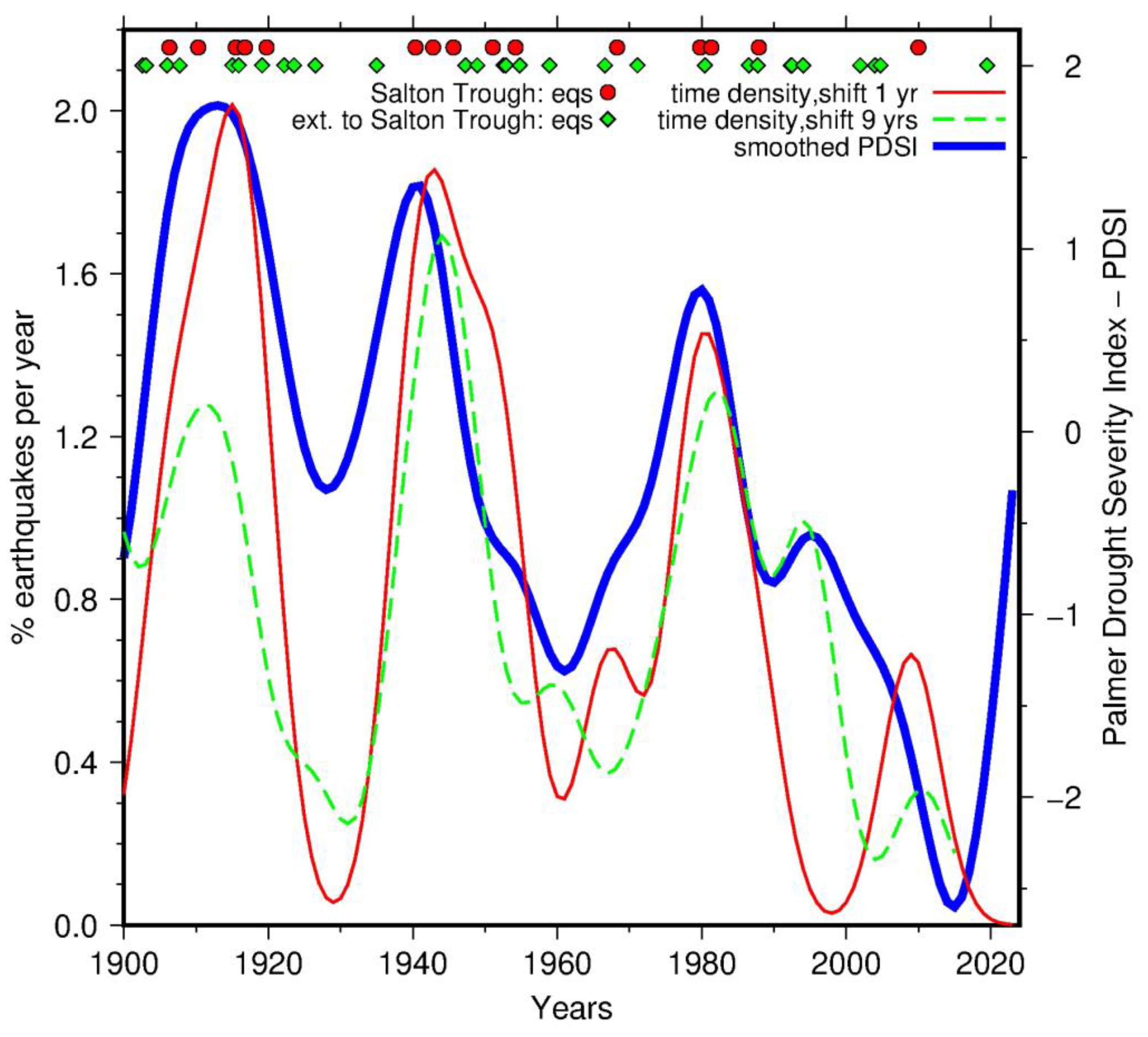
To test the existence of a large-scale seismic synchronization throughout Southern California, the same analysis was performed for the 30 mainshocks with Mw≥5.7 occurred inland externally to the Salton Trough area since 1900 (diamonds in the inset of Figure 1). In this case the estimated optimal time lag was 9 years, leading to significant positive correlation (b=0.31±0.11 with p=0.0038<0.05, case 3 in Table 1). The overall time relationship between the regional PDSI and the occurrence of earthquakes internally and externally to the Salton Trough area is summarized by the smoothed curves of Figure 4 (trend of the regional PDSI vs the smoothed time densities of earthquakes): after correction for the appropriate lags (one and 9 years), the curves appear well synchronized on the three main oscillations observed previously.
Discussion
Some critical points of the previous analysis are discussed in this section. The first is that trying different Δ-values for the same data set raises the multiple-testing issue, i.e., the possibility that at least one b deviates significantly from 0 purely by chance, a possibility that increases with the number of tests. Methods have been proposed to avoid this problem. They are based on reductions of the significance level that are proportional to the number of tests. The widely used Bonferroni correction (Perneger, 1998) was adopted here: if the number of tests is m and the desired overall significance level is α (in this work α=0.05 or 5%), each individual hypothesis would be tested at the adjusted significance level α/m. In the present work it is m=11 (they were tried the integer values of Δ between 0 and 10 years), so that the adjusted significance level is 0.05/11=0.0046. It is to note that the application of such penalization is not so straightforward. There is debate about its usefulness, necessity, and even its negative effects (Rothman, 1990; Perneger, 1998; Hooper, 2025), especially for preliminary exploratory studies such as the present one (Althouse, 2016). It has been pointed out that the adjustments are too conservative, with the consequent possibility of missing important findings. Rothman (1990) is for the extreme policy of making no adjustments, while Althouse (2016) is for the intermediate position of publishing all p-values as well as the significance levels of interest (with and without correction) and letting readers draw their own conclusions. In the present case, with m=11, the corrected significance level is 0.0046, so that the solutions previously found for PDSI in the two complementary areas (by Salton Trough and externally to it, cases 1 and 3 in Table 1) maintain the significance even after the adjustment (p=0.0024<0.0046 and p=0.0038<0.0046 respectively).
Another possible weakness of this study could result from the limited amount of data, with 15 earthquakes in 124 years. This problem also occurs in other similar studies: Rockwell and Klinger (2023), for example, use 16 earthquakes to investigate their possible relationship with 7 periods of flooding of Lake Cahuilla. Specifically for the logistic regression applied here, it has been shown that the Maximum Likelihood (ML) estimation of the parameters can be substantially biased for small samples [see (Stolte et al., 2024) for a general discussion], especially when, as pointed out by King and Zeng (2001), the number of positive cases is small compared to negative cases (15 years with an earthquake versus 119 years without earthquakes in the present data set). On the other hand, there is no consensus on the appropriate minimum sample size. A widely adopted empirical criterion is that of Peduzzi et al. (1996), which requires at least ten events per covariate (Events Per Variable, EPV), a condition that is met for the present BLR analysis (15 earthquakes and one covariate). There is a discussion about the validity of such criterion (Stolte et al., 2024). Here, it can only be noted that the earthquake data are close to the proposed limit, and some degree of bias is likely (the bias should be lower in the analysis external to the Salton Trough with 30 EPV). Techniques have been proposed to reduce the bias. The most consolidated method, suggested by many authors, is the Firth’s method (Firth, 1993), which incorporates a penalization term into the likelihood function. It was applied here using the package “logistf” (Heinz et al., 2025) for the R software system (R Core Team, 2012), trying only the lag of one years that was found to be optimal in the previous analysis (no Bonferroni correction for the significance level required). The results (case 4 in Table 1) are almost identical to those of the ML estimation (case 1 in Table 1) with b=0.38±0.12, significant at the 5% level (p=0.0023).
In this analysis, only the mainshocks are considered, to concentrate on variations of the background seismicity and avoid a possible spatial and temporal accumulation of earthquakes due to sequences of aftershocks. This selection, called declustering, is a critical phase of catalog processing, that is addressed in many publications proposing alternative methods. As described in the Data section, the declustering performed by Wang et al. (2009) with the ETAS model is used here, selecting the earthquakes with probability of independence pind>0.8 prior to the selection by magnitude. It is possible that different catalogs and different declustering methods lead to different results. Without claiming to settle this question definitively, a simple check was performed comparing the trend of the PDSI with M≥5.7 mainshocks drawn from the alternative catalog of Mueller (2019), specifically developed for the hazard maps of USGS. Here the declustering was performed using the distance and time window selection of Gardner and Knopoff (1974). The set of earthquakes in the Salton Trough area includes 15 earthquakes, 12 of which match the set from (Wang et al., 2009). The BLR for the single value Δ=1 (no Bonferroni adjustment required) confirms a positive b significant at the 5% level (Table 1, case 5): b=0.27±0.12 with p=0.027. Another subtle question concerns the declustering of an incomplete catalog, like that of (Wang, 2009). The ETAS model was run for all known earthquakes, but some earthquakes between magnitude 4.7 (the minimum threshold of the catalog) and 5.7 in the earliest part of the catalog are likely missing. It is possible that two earthquakes that are classified as independent (pind>0.8), are in fact linked in a seismic sequence by a chain of unreported, hidden earthquakes. This possible effect can be mitigated by increasing the probability of independence, e.g., from 0.8 to 0.9: in general, a larger pind implies a larger spatial/temporal distance between a couple of earthquakes classified as mainshocks, which would require a longer and less likely series of unreported earthquakes to link the couple in the same seismic sequence. With the threshold set to 0.9 and, consequently, the mainshocks slightly reduced from 15 to 13, the BLR estimation of b for Δ=1 is still positive and significant at the 5% level (b=0.38±0.14 with p=0.0055<0.05, case 6 in Table 1). Although this simple test reduces the doubt of a biased result, it does not eliminate it totally. It should be noted, however, that if a significant part of the earthquakes here assumed to be mainshocks were in fact linked by mutual triggering, one might conjecture that the Salton Trough (and, with a different timing, the entire Southern California), was struck in the past by three prominent seismic sequences, each spanning nearly a decade and tens of kilometers in space, and that in synchrony with groundwater recharge: in any case, a remarkable phenomenon that deserves to be reported to the scientific community for further investigation.
Conclusions
Both the BLR and the synchronization analysis based on the L-statistics indicate a significant time relationship between the occurrence of earthquakes and the increase in the PDSI. As shown by the smoothed time densities of earthquakes in Figure 2 and Figure 4, strong seismicity clustered near to three extremely wet periods (three main oscillations with peaks in 1916, 1944 and 1981), with a noticeable quiescence in the recent dry period. This behavior is consistent with that of the earthquakes occurred in the rest of Southern California (dashed line Figure 4), although anticipated by a few years. Both delays in respect to PDSI (1 and 9 years according to the BLR results, cases 1 and 3 in Table 1) are compatible with those of seismicity triggered by pore pressure propagation along faults and fractures with hydraulic diffusivity c between 0.1 and 10 m2/s as suggested by (Talwani et al., 2007). With seismicity in the area roughly distributed between 5 and 15 km in depth, the delay of one year determined for the Salton Trough is comparable with the delay estimated by (Mulargia and Bizzarri, 2014) for a simulation with c= 10 m2/s (200 days for the pore pressure pulse to travel 6 km), while the delay of 9 years externally to the Salton Trough is comparable with the delay estimated with c=0.1 m2/s (8 years to travel 12 km). In contrast, there is no significant relationship between seismicity and the SSL. In particular (Figure 3), clusters of strong earthquakes occurred for both high and low levels of the Salton Sea (around 1910 and 1950, respectively). Consequently, for the area and period studied here, groundwater increase is favored over water accumulation in the Salton Sea as a possible earthquake-triggering factor. Of particular interest is the trend of the last few decades (Figure 2 and Figure 4), when seismicity reached its minimum (just one earthquake in 38 years), almost coinciding with a series of prolonged drought phases, especially between 2000 and 2021, a period recognized by Williams et al. (2022) as the driest in the southwestern United States since at least 800 CE and classified as a “megadrought”. If the effect of meteoric water is confirmed by geophysical investigation, it could be postulated that the decrease in pore pressure caused by the megadrought has increased the frictional strength of faults, making strong earthquakes significantly less probable. The negative trend in groundwater partially reversed during the extremely wet season of early 2023; however, according to Mao et al. (2025), only about 25% of the groundwater lost since 2006 was recovered.
The analysis presented here has exploratory character. As pointed out in the Discussion, the statistical results may be biased by the limited data set and the difficulty to perform reliable declustering of an incomplete catalog. The use of an index such as the PDSI, which refers to water accumulation in the topsoil and not at depth, is also a limitation. Further studies are needed to confirm the estimated trends and to better understand the mechanisms of penetration and concentration of meteoric water at depth, and its interaction with the seismogenic faults.
Figure 4.
Comparison between the trend of PDSI and the time distribution of the Mw≥5.7 earthquakes occurred in the Salton Trough area since 1900 (circles) and those occurred externally to it in Southern California (diamonds, see their epicenters in the inset of Figure 1). The thin and the dashed curves represent the corresponding smoothed time densities of the earthquakes obtained by Gaussian kernel estimation with a bandwidth of 4 years (Bowman and Azzalini, 1997). They have been advanced by 1 and 9 years, respectively (i.e., the delays in respect to PDSI estimated by BLR analysis).
Data and Resources
Earthquake data for the period 2008-2023 came from the online PDE catalog of the USGS National Earthquake Information Center available at https://earthquake.usgs.gov/earthquakes/search/. All the other data used came from the published sources listed in the references. Statistical computation was performed using functions implemented for the R software system (R Core Team, 2012): the ‘’glm’’ function of the “MASS” package (Venables and Ripley, 2002) for binomial regression analysis with the Maximum Likelihood estimation of parameters; the “logistf” of the “LOGISTF” package (Heinze et al., 2025) for binomial regression analysis with the Firth’s method.
Acknowledgments
All the figures were produced using the Generic Mapping Tools (Wessel et al., 2019).
References
- Althouse, A.D. (2016). Adjust for multiple comparisons? It’s not that simple. Ann. Thorac. Surg, 101, 1644-1645. [CrossRef]
- Bettinelli, P., J. -P. Avouac, M. Flouzat, L. Bollinger, G. Ramillien, S. Rajaure, et al. (2008). Seasonal variations of seismicity and geodetic strain in the Himalaya induced by surface hydrology. Earth Planet. Sci. Lett. 266, 332–344. [CrossRef]
- Bollinger, L., F. Perrier, J.-P. Avouac, S. Sapkota, U. Gautam, and D. R. Tiwari (2007). Seasonal modulation of seismicity in the Himalaya of Nepal, Geophys. Res. Lett. 34, L08304. [CrossRef]
- Bowman, A. W. , and A. Azzalini (1997). Applied Smoothing Techniques for Data Analysis, Oxford Univ. Press, Oxford, United Kingdom.
- Bragato, P.L. (2021). Statistical Relationship Between the Decrease of Major Seismicity and Drought in Southern California Since 1900, Front. Earth Sci. 9, 790412. [Google Scholar] [CrossRef]
- Bragato, P.L. , and M. Sugan (2014). Decreasing Rate of M≥7 Earthquakes in the Northern Hemisphere since 1900, Seismological Res. Lett. 85, 1234–1242. [CrossRef]
- D’Agostino, N., F. Silverii, O. Amoroso, V. Convertito, F. Fiorillo, G. Ventafridda, et al. (2018). Crustal deformation and seismicity modulated by groundwater recharge of karst aquifers. Geophys. Res. Lett. 45, 12253–12262. [CrossRef]
- Dai, A. (2011). Characteristics and Trends in Various Forms of the Palmer Drought Severity Index during 1900-2008. J. Geophys. Res. 116, D12115. [CrossRef]
- De Luca, G., G. Di Carlo, and M. Tallini (2018). A record of changes in the Gran Sasso groundwater before, during and after the 2016 Amatrice earthquake, central Italy, Sci. Rep. 8, 15982. [CrossRef]
- Ellsworth, W.L. (2013). Injection-induced Earthquakes, Science 341, 1225942. [CrossRef]
- Firth, D. (1993). Bias Reduction of Maximum Likelihood Estimates. Biometrika, 80, 27–38.
- Gardner, J. K. , and L. Knopoff (1974). Is the sequence of earthquakes in southern California, with aftershocks removed, Poissonian? Bull. Seismol. Soc. Am, 64, 1363–1367. [CrossRef]
- Hainzl, S., T. Kraft, J. Wassermann, H. Igel, and E. Schmedes (2006). Evidence for rainfall-triggered earthquake activity. Geophys. Res. Lett, 33, L19303. [CrossRef]
- Heinze G, Ploner M, Jiricka L, Steiner G (2025). logistf: Firth’s Bias-Reduced Logistic Regression (1.26.1) [R package]. https://CRAN.R-project.org/package=logistf. [CrossRef]
- Hooper, R. (2025). To adjust, or not to adjust, for multiple comparisons, Journal of Clinical Epidemiology 180, 111688. [CrossRef]
- Hill R.G., M. , Weingarten, T.K. Rockwell, and Y Fialko (2023). Major southern San Andreas earthquakes modulated by lake-filling events, Nature 618, 761-766. [CrossRef]
- Huang, L.-S., J. McRaney, T.-L. Teng, and M. Prebish (1979). A preliminary study on the relationship between precipitation and large earthquakes in Southern California. Pageoph 117, 1286–1300. [CrossRef]
- Kraft, T., J. Wassermann, E. Schmedes, and H. Igel (2006). Meteorological triggering of earthquake swarms at Mt. Hochstaufen, SE-Germany. Tectonophysics, 424, 245–258. [CrossRef]
- King, G., and L. Zeng (2001). Logistic regression in rare events data. Political Analysis 9, 137-163. [CrossRef]
- Lindsey, E.O., and Y. Fialko (2016). Geodetic constraints on frictional properties and earthquake hazard in the Imperial Valley, Southern California, J. Geophys. Res. 121, 1097-1113. [CrossRef]
- Liritzis, I. , and B. Petropoulos (1994). The relationship between precipitation and shallow earthquakes (M≥5 1/2) revisited, Europ. Seism. Comm. XXIV. Gen. Assembly 1, 1973–1979.
- Liritzis, Y., and B. Petropoulos (1992). A preliminary study of the relationship between large earthquakes and precipitation for the region of Athens, Greece, Earth Moon Planet 57, 13–21. [CrossRef]
- Luttrell, K., D. Sandwell, B. Smith-Konter, B. Bills, and Y. Bock (2007). Modulation of the earthquake cycle at the southern San Andreas Fault by lake loading, J. Geophys. Res. 112, B08411. [CrossRef]
- Mao, S., W. L. Ellsworth, Y. Zheng, and G. C. Beroza1 (2025). Depth-dependent seismic sensing of groundwater recovery from the atmospheric-river storms of 2023. Science. [CrossRef]
- Mueller, C. S. (2019). Earthquake Catalogs for the USGS National Seismic Hazard Maps, Seismol. Res. Lett. 90, 251–261. [CrossRef]
- Mulargia, F., and A. Bizzarri (2014). Anthropogenic triggering of large earthquakes. Sci. Rep. 4, 6100. [CrossRef]
- Oglesby, L. C. (2005). The Salton Sea: geology, history, potential problems, politics, and possible futures of an unnatural desert salt lake, Memoirs of the Southern California Academy of Sciences 10, Los Angeles, CA.
- Palmer, W. C. (1965). Meteorological Drought, Res. Paper No.45, Dept. of Commerce, Washington, D.C.
- Panda, D., B. Kundu, V.K. Gahalaut, R. Bürgmann, B. Jha, R. Asaithambi, et al. (2018). Seasonal modulation of deep slow-slip and earthquakes on the main Himalayan thrust, Nat. Commun. 9, 4140. [CrossRef]
- Peduzzi, P., J. Concato, E. Kemper, T.R. Holford, and A.R. Feinstein (1996). A simulation study of the number of events per variable in logistic regression analysis, J. Clin. Epidemiol 49, 1373–1379. [CrossRef]
- 35. van Smeden M, Moons KG, de Groot JA, et al. Sample size.
- Perneger, T.V. (1998). What’s wrong with Bonferroni adjustments. BMJ, 316, 1236-1238. [CrossRef]
- R Core Team (2012), R: A Language and Environment for Statistical Computing. R Foundation for Statistical Computing, Vienna, Austria.
- Rockwell, T.K. , Meltzner A.J., Haaker E.C., Madugo, D. (2022). The late Holocene history of Lake Cahuilla: two thousand years of repeated fillings within the Salton Trough, Imperial Valley, California. Quaternary Science Reviews, 282, 107456. [CrossRef]
- Rockwell, T.K. , and Y. Klinger (2023). 2000 yrs of earthquakes inferred from subsidence events on the Imperial fault, California: effect of lake-level changes and implication for variable slip rates, Earth and Planetary Science Letters 618, 118271. [CrossRef]
- Rothman, K.J. (1990). No adjustments are needed for multiple comparisons. Epidemiol, 1, 43-46. [CrossRef]
- Scharer, K.M. , and D. Yule (2020). A maximum rupture model for the Southern San Andreas and San Jacinto Faults, California, derived from paleoseismic earthquake ages: observations and limitations, Geophys. Res. Lett. 47, e2020GL088532. doi.org:10.1029/2020GL088532.
- Stolte, M., S. Herbrandt, and U. Ligges (2024). A comprehensive review of bias reduction methods for logistic regression. Statistics Surveys 18, 139–162. [CrossRef]
- Talwani, P., L. Chen, and K. Gahalaut (2007). Seismogenic Permeability,ks. J. Geophys. Res. 112, B07309. [CrossRef]
- Tostrud, M.B. (1997). The Salton Sea, 1906-1996, computed and measured salinities and water levels (draft), Colorado River Board of California, Glendale. California.
- Venables, W. N. , and B.D. Ripley (2002). Modern Applied Statistics with S. 4th Ed, Springer, New York.
- Vose, R. S., S. Applequist, M. Squires, I. Durre, M.J. Menne, C.N. Williams, et al. (2014). Improved Historical Temperature and Precipitation Time Series for U.S. Climate Divisions, J. Appl. Meteorol. Climatol. 53, 1232–1251. [CrossRef]
- Wang, Q., D. D. Jackson, and Y.Y. Kagan (2009). California Earthquakes, 1800-2007: a unified catalog with moment magnitudes, uncertainties, and focal mechanisms, Seism. Res. Lett. 80, 446–457. [CrossRef]
- Wang, C-Y., and Manga, M. (2010). Earthquakes and Water. Springer-Verlag, Berlin and Heidelberg, Germany. [CrossRef]
- Wessel, P., J. F. Luis, L. Uieda, R. Scharroo, F. Wobbe, W.H.F. Smith, and D. Tian (2019). The Generic Mapping Tools version 6, Geochemistry, Geophys., Geosystems 20, 5556–5564. [CrossRef]
- Williams, A. P., I. C. Benjamin, and J.E. Smerdon (2022). Rapid intensification of the emerging southwestern North American megadrought in 2020–2021. Nat. Clim. Change. [CrossRef]
- Zaliapin, I. , and Y. Ben-Zion (2020). Earthquake declustering using the nearest-neighbor approach in space-time-magnitude domain. J. Geophys. Res, 125, e2018JB017120. [CrossRef]
- Zhuang, J., Y. Ogata, Y., and D. Vere-Jones (2002). Stochastic declustering of space-time earthquake occurrences, J. Am. Stat. Assoc. 97, 369–380. [CrossRef]
Figure 1.
Salton Trough area with the indication of the existing Salton Sea and of the ancient Lake Cahuilla. The circles are the epicenters of the Mw≥5.7 earthquakes since 1900 considered for the analysis. The diamonds in the inset are the epicenters of the Mw≥5.7 mainshocks that occurred inland in Southern California externally to the Salton Trough area since 1900.
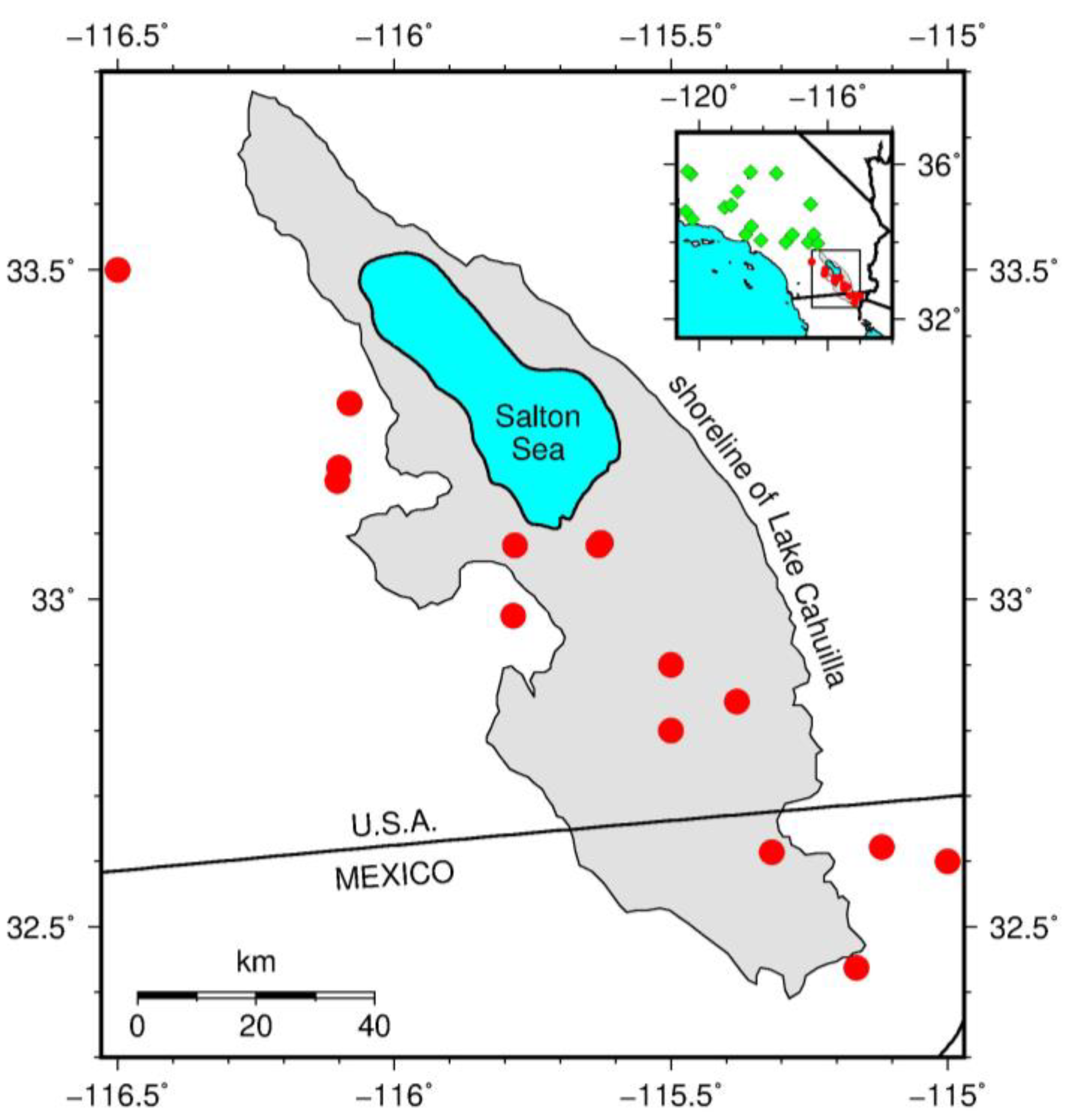
Figure 2.
Magnitude/time distribution of the Mw≥5.7 mainshocks used in the analysis (vertical bars) compared with trend of PDSI (thin continuous line) and its smoothed version by Gaussian filtering (Bowman and Azzalini, 1997) (thick continuous line). The black line is the smoothed time density of the earthquakes obtained by Gaussian kernel estimation with a bandwidth of 4 years (Bowman and Azzalini, 1997).
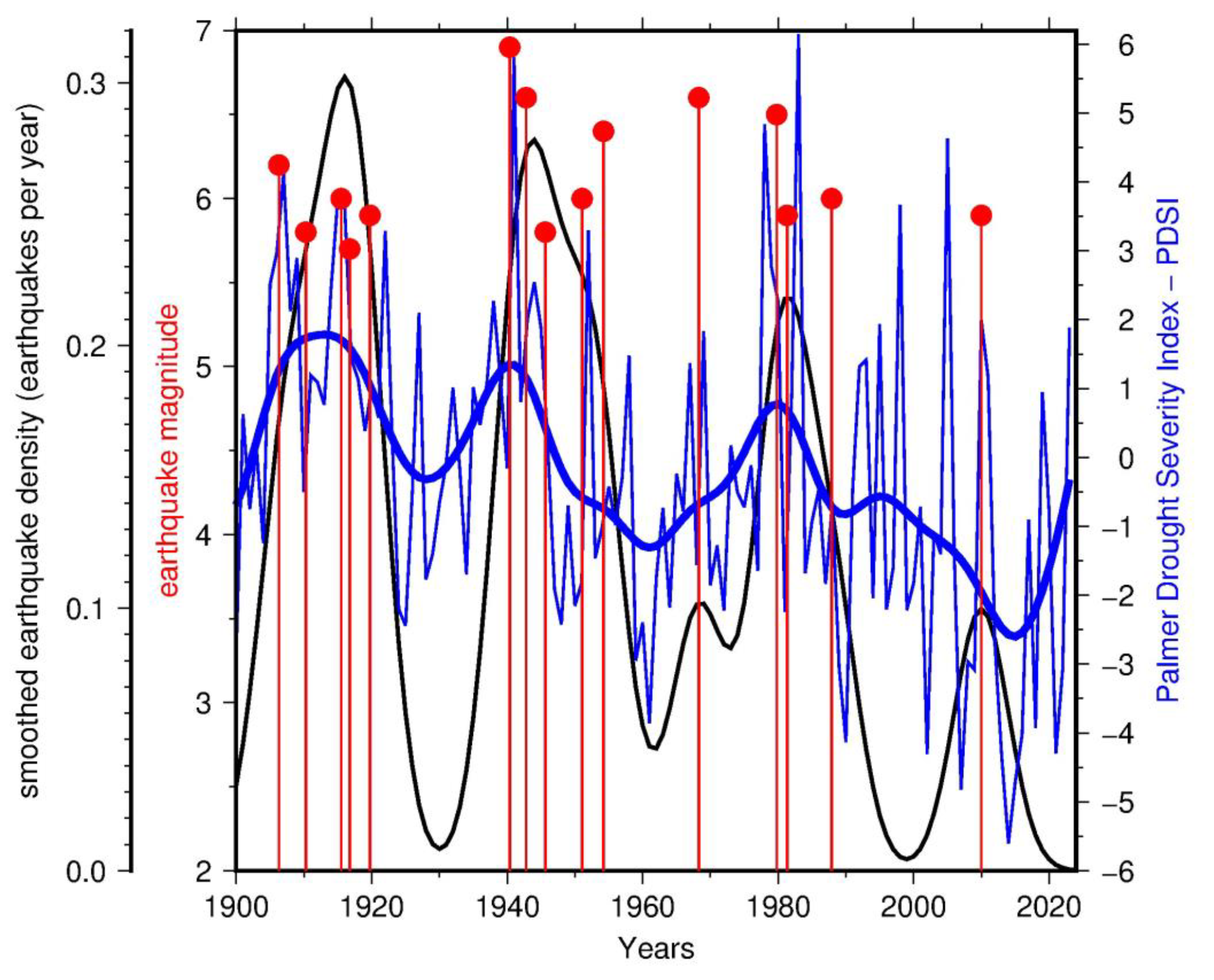
Figure 3.
Magnitude/time distribution of the Mw≥5.7 mainshocks used in the analysis (vertical bars) compared with the trend of the Salton Sea Level (thin continuous line).
Figure 3.
Magnitude/time distribution of the Mw≥5.7 mainshocks used in the analysis (vertical bars) compared with the trend of the Salton Sea Level (thin continuous line).
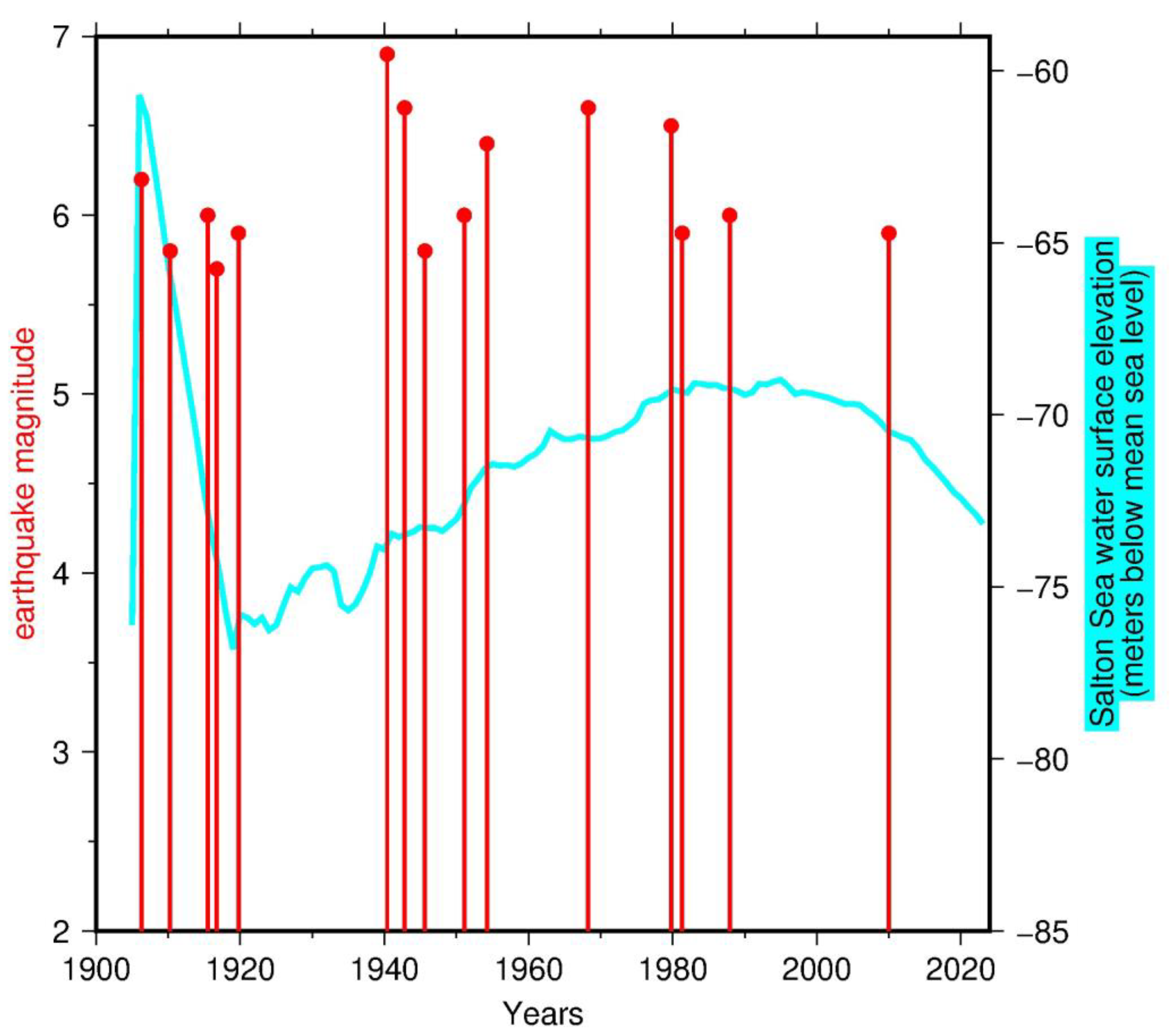

Table 1.
Results of binary logistic regression for different data sets and regression methods.
| case | earthquake catalog | covar. | n. eqs | period (yrs) |
m (n.tests) |
lag (yrs) |
a | b | pb | Bonferroni correction 0.05/m |
|---|---|---|---|---|---|---|---|---|---|---|
| 1 | Salton Trough, M≥5.7 | PDSI | 15 | 1900-2023 | 11 | 1 | -2.19±0.33 | 0.40±0.13 | 0.0024 | 0.0046 |
| 2 | Salton Trough, M≥5.7 | SSL | 15 | 1900-2023 | 11 | 0 | -4.36±5.67 | 0.09±0.08 | 0.2647 | - |
| 3 | out of Salton Trough,M≥5.7 | PDSI | 30 | 1900-2023 | 11 | 9 | -1.42±0.25 | 0.31±0.11 | 0.0038 | 0.0046 |
| 4 | Salton Trough, M≥5.7 Firth’s bias reduction |
PDSI | 15 | 1900-2023 | 1 | 1 | -2.12±0.32 | 0.38±0.12 | 0.0023 | - |
| 5 | Salton Trough, M≥5.7 cat. (Mueller 2019) |
PDSI | 15 | 1900-2023 | 1 | 1 | -2.06±0.30 | 0.27±0.12 | 0.0270 | - |
| 6 | Salton Trough, M≥5.7 pind>0.9 |
PDSI | 13 | 1900-2023 | 1 | 1 | -2.34±0.34 | 0.38±0.14 | 0.0055 | - |
Disclaimer/Publisher’s Note: The statements, opinions and data contained in all publications are solely those of the individual author(s) and contributor(s) and not of MDPI and/or the editor(s). MDPI and/or the editor(s) disclaim responsibility for any injury to people or property resulting from any ideas, methods, instructions or products referred to in the content. |
© 2025 by the authors. Licensee MDPI, Basel, Switzerland. This article is an open access article distributed under the terms and conditions of the Creative Commons Attribution (CC BY) license (http://creativecommons.org/licenses/by/4.0/).
Copyright: This open access article is published under a Creative Commons CC BY 4.0 license, which permit the free download, distribution, and reuse, provided that the author and preprint are cited in any reuse.


