
Submitted:
21 October 2025
Posted:
23 October 2025
You are already at the latest version
Abstract
The representation of three-dimensional (3D) shapes from point clouds remains a fundamental challenge in computer vision.
A common approach decomposes 3D objects into interpretable geometric primitives, enabling compact, structured, and efficient representations.
Building upon prior frameworks, this study introduces an enhanced unsupervised deep learning approach for 3D shape representation using superquadrics.
The proposed framework fits a set of superquadric primitives to 3D objects through a fully integrated, differentiable pipeline that enables efficient optimization and parameter learning, directly extracting geometric structure from 3D point clouds without requiring ground-truth segmentation labels.
This work introduces three key advancements that substantially improve representation quality, interpretability, and evaluation rigor:
(1) a uniform sampling strategy that enhances training stability compared with random sampling used in earlier models;
(2) an overlapping loss that penalizes intersections between primitives, reducing redundancy and improving reconstruction coherence; and
(3) a novel evaluation framework comprising \emph{Primitive Accuracy}, \emph{Structural Accuracy}, and \emph{Overlapping Percentage} metrics.
This new metric design transitions from point-based to structure-aware assessment, enabling fairer and more interpretable comparison across primitive-based models.
Comprehensive evaluations on benchmark 3D shape datasets demonstrate that the proposed modifications yield coherent, compact, and semantically consistent shape representations, establishing a robust foundation for interpretable and quantitative evaluation in primitive-based 3D reconstruction.
Keywords:
3D shape representation
; superquadrics
; deep learning
; unsupervised learning
; point clouds
; geometric modeling
1. Introduction
The representation of three-dimensional (3D) shapes from point clouds is a fundamental challenge in visual computing, underpinning applications in shape abstraction, geometric modeling, and robotic perception [1,2,3]. A common approach to achieving compact and structured representations is to decompose 3D objects into a set of interpretable geometric primitives. Unlike traditional segmentation tasks that partition a shape into semantically meaningful components, primitive-based decomposition reconstructs the overall geometry using a limited number of parametric forms. Among these, superquadrics—a versatile family of parametric surfaces—are widely adopted for their ability to model a broad range of geometric shapes [4].
In this work, a deep learning framework for superquadric-based unsupervised three-dimensional (3D) shape decomposition is proposed. Leveraging a differentiable parameterization, the approach fits superquadric primitives to point clouds in a fully integrated pipeline, extracting meaningful structures without requiring ground-truth segmentations. We build upon prior efforts, including Paschalidou et al. [5] and our previous work [6], introducing three key advancements: (i) a uniform sampling strategy for enhanced training stability, (ii) an overlapping loss to reduce primitive redundancy, and (iii) a comprehensive evaluation framework introducing Structural Accuracy, Primitive Accuracy, and Overlapping Percentage metrics for improved quantitative and structural assessment. Evaluated on benchmark datasets, we show that the proposed method achieves more coherent and accurate shape decompositions than previous deep learning frameworks. A detailed discussion of these contributions and their relationship to prior work is provided below.
Paper Organization. The remaining paper is structured as follows: Section 2 reviews prior work on 3D shape representation, focusing on key milestones in primitive-based modeling and deep learning approaches. It also highlights how our contributions address the limitations identified in these methods. Section 3 provides a theoretical overview of superquadrics and their mathematical formulations, which form the foundation of our 3D shape decomposition framework. Section 4 describes enhancements to the loss functions for superquadric-based 3D shape representation introduced in our earlier framework, focusing on improved primitive alignment and structural coverage. Section 5 details the neural architecture, training setup, and optimization constraints employed in our framework. Section 6 presents the enhanced loss function, which integrates a uniform sampling strategy and an overlapping loss to improve segmentation accuracy and reduce primitive redundancy in 3D shape representation. Section 7 evaluates the model’s performance through quantitative and qualitative experiments on the ShapeNet dataset, comparing sampling strategies, overlapping loss effects, and segmentation quality using the proposed Structural Accuracy, Primitive Accuracy, and Overlapping Percentage metrics. Section 8 summarizes our advancements in superquadric-based 3D shape representation, including the overlapping loss, uniform sampling strategy, and evaluation framework, and outlines future research directions for enhancing geometric and semantic modeling.
2. Related Work and Review of Our Contributions
This section begins with an overview of three-dimensional (3D) shape representation, highlighting key milestones that define the context of the present work. Subsequently, we discuss in detail the two most relevant prior works that directly motivate and inform our proposed framework. Finally, our own contributions are reviewed within this context to clarify how they address existing limitations and extend the state of the art.
2.1. Some Milestones in 3D Shape Representation
Early three-dimensional (3D) shape representations in visual computing often relied on geometric primitives to balance interpretability and computational efficiency [7,8,9]. Primitive-based modeling—using parametric shapes such as spheres, cuboids, ellipsoids, or superquadrics—provides a structured abstraction of 3D geometry, ensuring that the overall shape can be reconstructed from a compact set of parameters [4,10].
Early methods such as polyhedral models [11] and generalized cylinders [12] established foundational principles for shape abstraction but were constrained by the computational and sensing capabilities of their time. As the field matured, optimization-based models gained prominence, offering improved flexibility and robustness for representing complex or noisy 3D data [8,13]. Superquadrics [7], though rooted in classical modeling, gained renewed attention for their ability to represent a broad range of convex shapes using only a few parameters [4]. Optimization-based fitting techniques were subsequently developed to align superquadric primitives with point cloud or range data [14,15,16]. These methods were often refined using the Iterative Closest Point (ICP) algorithm [17], which iteratively aligns 3D shapes by minimizing the distance between corresponding surface points.
Primitive-based decompositions are particularly valuable for downstream tasks such as robotic manipulation, where identifying graspable components through geometric primitives can enhance planning and interaction strategies [18]. Furthermore, reasoning about object shape configurations benefits from structured representations that capture compositional relationships, such as part-based or grammar-based models [19]. Recent learning-based approaches extend this line of work by automatically discovering primitive decompositions and hierarchical part structures directly from raw 3D data, enabling improved understanding of articulated objects and supporting tasks such as robotic grasping and assembly [20]. Classical primitive-based methods have thus laid the foundation for modern deep learning techniques in 3D shape representation. The following section highlights key milestones in these developments, emphasizing different neural network architectures and representation paradigms.
Implicit neural representations describe three-dimensional (3D) shapes as continuous functions over space, rather than as discrete elements such as voxels or meshes.
In this approach, a shape is not defined explicitly but instead emerges as the level set of a learned function. For example, DeepSDF [21] learns a continuous signed distance function in which each query point in 3D space is assigned its signed distance to the nearest surface. Occupancy Networks [22] learn a binary-valued function that classifies each point as inside or outside of an object. NeRF [23], originally developed for novel view synthesis, represents volumetric geometry through continuous radiance fields that implicitly encode surface and appearance information. These models are typically trained in a supervised manner. Depending on the representation, supervision may involve ground-truth signed distance values for sampled 3D points, as in DeepSDF, or ground-truth occupancy labels derived from mesh or volumetric data, as in Occupancy Networks. In both cases, accurate ground-truth shape data or posed views are required for effective training. However, while deep implicit methods excel at producing high-fidelity reconstructions, they typically encode geometry in a dense, global latent space. Although powerful for capturing fine surface details, this representation offers limited transparency regarding the object’s composition into interpretable components or functionally meaningful parts. As highlighted by Sitzmann et al. [24], disentangling meaningful part-level structure or semantics from such dense neural fields remains challenging, particularly when aiming for structured or compositional abstractions.
Volumetric convolutional neural networks (CNNs), such as VoxNet [25] and OctNet [26], represent three-dimensional (3D) shapes using voxel grids and apply 3D convolutions to learn volumetric features. These supervised methods enable grid-structured learning but suffer from high memory and computational demands, a common limitation of volumetric representations that constrains achievable resolution. Notably, the unsupervised approach of Paschalidou et al. [5], discussed in greater detail below, exhibits similar scalability constraints, as it also relies on volumetric sampling within a grid-based representation.
Graph-based or mesh-based convolutional neural networks (CNNs) operate on point clouds or meshes representing object surfaces. Structured surfaces, such as meshes, provide explicit vertex connectivity through edges, enabling convolution over well-defined local neighborhoods. In contrast, unstructured surfaces, such as raw point clouds, lack this topology and require neighborhood inference to establish local relationships. Methods such as GCNNs [27] and mesh-based learning frameworks [28] enable learning on structured surfaces and are particularly effective for deformable shape modeling.
Point-based methods, such as PointNet [2] and Superpoint Graph (SPG) [29], directly process raw, unstructured point sets, often obtained from LiDAR or RGB-D scans. These methods often require ground-truth labels for supervised training, such as semantic part annotations or object class labels, depending on the application. Unlike images, point clouds lack a fixed spatial ordering, requiring networks to be invariant to permutations of input points. This is typically achieved using symmetric aggregation functions, such as max-pooling or average-pooling, which combine per-point features into a global shape descriptor invariant to point ordering. Point-based architectures are widely adopted in robotics and autonomous systems because they naturally handle sparse and irregular 3D data. This makes point-based methods well-suited for tasks such as object recognition, part segmentation, and grasp planning in real-world environments.
2.2. Shape Primitives and Deep Learning
Primitive-based models represent three-dimensional (3D) shapes as compositions of parametric elements. In deep learning–based approaches, a neural network predicts the parameters of geometric primitives—such as cuboids, spheres, or superquadrics—that together approximate the target object. Such structured representations yield compact shape descriptions and can facilitate semantic interpretability, as each primitive may correspond to a distinct part or functional component of the object.
Recent deep learning methods combine neural encoders with differentiable primitive decoders to operationalize this concept within end-to-end trainable frameworks. For example, Tulsiani et al. [30] proposed a supervised volumetric convolutional neural network (CNN) that voxelizes the input shape and processes it with 3D convolutions to predict assemblies of cuboid primitives. This design leverages the regular Euclidean structure of voxel grids to extend convolution operations from two to three dimensions. From the learned volumetric features, the decoder predicts cuboid parameters—including position, scale, and orientation—for an assembly that approximates the target shape. Paschalidou et al. [5] extended this volumetric framework by fitting differentiable parametric implicit surfaces to sparse 3D point data in an unsupervised manner. Their model employs differentiable inside–outside functions to compute point-to-surface distances, directly optimizing primitive parameters without requiring labeled part annotations. Although volumetric CNNs, as used in these works, offer straightforward representations and support spatial reasoning, they are computationally and memory intensive at high resolutions. This limitation has motivated subsequent research to explore point-based encoders and implicit decoders for more scalable 3D modeling.
Building on the framework proposed in [5], Paschalidou et al. introduced Neural Parts [31], a more flexible representation in which each primitive is defined by an invertible neural network (INN). The method takes as input a three-dimensional (3D) point cloud that is encoded using a PointNet++ [2] backbone to extract both local and global geometric features. The resulting latent representation is then mapped by the INN to part-level latent variables, which are decoded into implicit occupancy functions that describe the geometry of each part. This pipeline enables highly expressive, non-parametric part geometries and achieves semantic consistency across instances without requiring explicit supervision. However, the primitive shapes are no longer defined by explicit parametric equations but are instead encoded within neural weights, thereby limiting interpretability and complicating analytical assessment.
Following Neural Parts, several subsequent studies have expanded upon interpretable and unsupervised three-dimensional (3D) shape decomposition. Yang and Chen [32] proposed an unsupervised cuboid-based abstraction framework employing geometric regularization to improve structural consistency. Xu et al. [33] developed a part-regularized reconstruction framework incorporating structural priors to enhance decomposition quality. Yuldasheva et al. [34] revisited classical superquadric-based decomposition with modern optimization strategies, reaffirming the importance of parametric primitives in unsupervised shape analysis. Li et al. [35] introduced SfmCAD, a method that jointly learns structural and free-form primitives to model CAD-like object geometries. Li et al. [36] further proposed a shared-latent representation that enables joint analysis and reconstruction across multiple object categories. Li et al. [37] presented PASTA, a part-aware generative model that explicitly controls structural composition through learned part embeddings. Chen and Cheng [38] demonstrated that procedurally generated 3D datasets can effectively train models to generalize structured representations to real-world objects. Kobsik et al. [39] introduced a fine-to-coarse cuboid abstraction network that hierarchically learns part-level decompositions in an unsupervised manner. Ye et al. [40] proposed PrimitiveAnything, a foundation-model-based framework that abstracts 3D scenes into semantically meaningful primitives, bridging geometric abstraction with multimodal reasoning.
Collectively, these studies highlight a growing focus on interpretable and semantically guided three-dimensional (3D) abstractions. Our work complements this line by adopting an analytically defined, fully unsupervised formulation grounded in superquadrics, explicitly bridging classical geometric interpretability with modern deep learning architectures.
Recent approaches such as Neural Parts [31], PASTA [37], and PrimitiveAnything [40] have introduced flexible and multimodal paradigms for part decomposition, frequently leveraging large-scale supervision or pretrained foundation models. In contrast, our work emphasizes a fully unsupervised and analytically interpretable framework grounded in superquadrics.
For methodological consistency, our experimental comparisons focus on the family of superquadric-based methods, including the baseline formulation [5] and our previous extension [6], and aim to clearly highlight the improvements introduced in sampling, overlap handling, and evaluation metrics. The following subsections examine in detail the two most relevant sources of previous work for this study.
2.3. Paschalidou et al.[5]: Learning 3D Shape Parsing Beyond Cuboids
Paschalidou et al. [5] proposed a novel approach to unsupervised three-dimensional (3D) shape representation and decomposition using volumetric convolutional neural networks (CNNs) applied to voxel grids. Their network predicts the parameters of multiple superquadric primitives directly from voxelized representations of 3D objects. Due to the high computational cost of volumetric CNNs, their experiments were constrained to low-resolution voxel grids, limiting both the complexity and diversity of the reconstructed shapes. The primary contributions of Paschalidou et al.’s work include:
- Superquadrics for 3D Shape Representation: They extended the use of superquadrics by enabling the decomposition of complex 3D shapes into multiple parametric primitives, capturing fine part-level structure and geometric variation. Unlike earlier cuboid-based decomposition methods [30], their approach models curvature and irregularities more effectively through the parametric flexibility of superquadrics, resulting in improved segmentation and part delineation while maintaining compact and interpretable representations.
- End-to-End Learning Pipeline: The authors proposed an end-to-end differentiable learning pipeline in which the parameters of superquadric models are directly learned from voxelized shape representations. Because the entire model—including both optimization and shape parameter estimation—is differentiable, it can be trained via gradient-based optimization without relying on manually crafted features. This design allows for flexible and adaptive 3D shape representation.
- Qualitative Evaluation: Through qualitative experiments, Paschalidou et al. demonstrated that their superquadric-based method outperformed the traditional cuboid-based approach [30], achieving visually superior reconstructions and more coherent primitive assemblies.
Their results suggest that superquadrics are particularly suitable for representing objects with curved or elongated features, such as furniture, airplanes, and other real-world categories. However, a key limitation of their approach is the tendency of superquadric primitives to exhibit excessive overlap when representing complex shapes.
Figure 1 provides a qualitative comparison across various object categories, illustrating the limitations of the baseline method [5]. Excessive primitive overlap is particularly evident in objects with intricate geometries, such as chairs, tables, mugs, and bags, where the model often fails to delineate structural boundaries accurately, causing primitives to extend beyond their intended regions.
Summary of Challenges.
Paschalidou et al. [5] demonstrated the potential of superquadrics in capturing geometric structure and proposed an end-to-end learning framework for 3D shape decomposition. Nevertheless, their method exhibits several key limitations that affect both performance and scalability, summarized as follows:
- Unstructured Random Initialization of Superquadrics. The optimization process initializes superquadric parameters randomly (e.g., from uniform or Gaussian distributions) without incorporating prior geometric constraints. In contrast to structured initialization strategies such as Kaiming initialization [41], which promote stability in neural network training, this unstructured parameter initialization can lead to inconsistent optimization behavior. Consequently, decompositions may vary across runs and often converge to suboptimal configurations, particularly in shapes with complex geometry.
- Lack of Quantitative Evaluation Metrics. While the method presents compelling qualitative results, it lacks rigorous quantitative evaluation metrics, making objective assessment of reconstruction and segmentation performance difficult.
- Loss Function Limitations. Although effective for parameter optimization, the baseline loss function does not penalize geometric overlap between primitives, leading to redundant representations and reduced segmentation accuracy, especially for objects with fine-grained structural details.
- Voxel Grid Representation. The reliance on voxelized inputs and volumetric CNNs results in substantial computational and memory overhead. This constraint restricts the achievable resolution and limits the complexity of shapes that can be effectively represented, as high-resolution voxel grids are prohibitively resource-intensive.
A subsequent method by Paschalidou et al. [31], known as Neural Parts, extends the 2019 superquadric-based framework but introduces a fundamentally different representation paradigm. Neural Parts employs invertible neural networks (INNs) combined with latent variable modeling to learn hierarchical 3D shape abstractions, enabling bijective mappings between canonical shapes and target part geometries for greater flexibility. Specifically, the method takes as input a three-dimensional (3D) point cloud of the object, which is first encoded by a PointNet++-based encoder [2] into a global latent representation. This latent representation is then processed through the INN to generate part-level latent variables, which are subsequently decoded via implicit occupancy functions to reconstruct the geometry of each part.
This pipeline allows Neural Parts to model richer, non-parametric part geometries compared to the analytic superquadric formulation. While PointNet++ [2] extracts geometric features such as local curvature and spatial context, the INN disentangles these into part-specific latent embeddings, which are decoded into implicit neural surfaces. This enables accurate part-level decompositions, such as distinguishing between a chair leg and a spherical component placed above it; however, the resulting parts are represented as implicit neural functions rather than analytic primitives. Consequently, the method transitions from explicit parametric superquadric formulations to implicit neural mappings. This shift offers greater flexibility but sacrifices the closed-form analytic geometry of superquadrics, which in turn reduces interpretability and limits direct applicability in domains such as CAD modeling, physics simulation, and analytical surface manipulation.
2.4. Our previous work: Unsupervised 3D Shape Description Using Superquadrics
In our previous work [6], we extended the superquadric-based deep learning framework introduced by Paschalidou et al. [5], introducing several key modifications to address limitations related to training stability, primitive overlap, and computational efficiency. In contrast to Neural Parts [31], our work retains the explicit parametric superquadric representation, emphasizing its compactness, geometric interpretability, and precise analytical control. The primary advancements introduced in our work [6] include:
- Improved Loss Function. We redesigned the loss formulation to enhance shape representation accuracy by better balancing compactness and reconstruction fidelity. The modified loss improved segmentation coherence and overall geometric consistency, as discussed in detail in Section 4.
- PointNet-Based Feature Extraction. Instead of relying on computationally expensive volumetric CNNs widely used in earlier works on 3D shape processing [5,42,43,44], we adopted a PointNet-based encoder [2] to directly process point cloud data. This design eliminates the need for voxelization, substantially reducing computational overhead while preserving essential geometric features, thus improving both scalability and efficiency.
- Cyclic Learning Rate. To improve training dynamics, we incorporated the cyclic learning rate strategy [45], which facilitates faster convergence and helps the optimizer escape local minima, enhancing overall network stability.
- Kaiming Weight Initialization. We applied Kaiming weight initialization [41] to enhance training stability by maintaining consistent gradient flow, leading to more reliable convergence across runs.
Collectively, these contributions [6] refined the superquadric-based framework of Paschalidou et al. [5], achieving improved segmentation coherence, higher reconstruction fidelity, and enhanced computational robustness.
Despite these improvements, our previous model still exhibited moderate overlap in specific object categories, particularly those with elongated or complex geometric structures (e.g., chairs or tables). In such cases, superquadric primitives tended to extend beyond their intended regions, resulting in segmentation inaccuracies that limited overall decomposition precision.
2.5. Our Contributions in this Paper in Detail
Building upon our previous work [6], this study introduces several methodological and conceptual innovations that advance unsupervised superquadric-based 3D shape representation. The proposed framework enhances segmentation consistency, minimizes primitive overlap, and establishes a novel, structure-aware evaluation methodology that enables more interpretable and reproducible comparison of primitive-based reconstruction models. Our main contributions are summarized as follows:
- Novel Structure-Aware Evaluation Framework. Traditional evaluations of primitive-based reconstruction rely on surface-level metrics such as Chamfer Distance or Earth Mover’s Distance, which capture geometric proximity but ignore structural coherence and primitive correspondence. To overcome these limitations, we propose a comprehensive evaluation framework that integrates three new complementary metrics: Primitive Accuracy (PA), Structural Accuracy (SA), and Overlapping Percentage (OP). This framework represents a conceptual shift from point-based to primitive-based evaluation, enabling direct assessment of both part-level fidelity and global structural alignment. It provides a transparent, quantitative basis for comparing primitive-based models and sets a new benchmark for interpretable 3D reconstruction.
- Overlapping Loss for Non-Intersecting Superquadrics. Previous methods, including Paschalidou et al. [5], did not explicitly constrain overlapping between superquadric primitives, often leading to redundant or ambiguous representations. We introduce a novel overlapping loss that penalizes spatial intersections between primitives, thereby promoting exclusive spatial partitioning and improving segmentation coherence. The Overlapping Percentage metric quantitatively assesses overlap reduction, providing a consistent measure of inter-primitive separation quality.
- Primitive- and Structural-Level Accuracy Measures. We introduce two complementary accuracy measures to capture distinct aspects of reconstruction quality. Structural Accuracy quantifies the proportion of input points accurately covered by the predicted primitives, reflecting global structural fidelity. Primitive Accuracy evaluates how well each superquadric aligns with its corresponding input region, capturing local geometric precision and identifying poor fits. Together, these measures provide the first unified framework for analyzing both global coverage and local alignment in superquadric-based reconstruction.
- Uniform Sampling Strategy. Previous studies, including Paschalidou et al. [5], Livne et al. [46], and our earlier work [6], employed random or heuristic surface sampling approaches. Such methods often produced uneven point distributions, causing unstable optimization and inconsistent training outcomes. We propose a uniform surface sampling strategy that maintains balanced point distributions across primitives by adaptively adjusting density according to local curvature. This results in smoother gradients, improved training stability, and enhanced reconstruction coherence.
- Evaluation on Complex and Realistic Geometries. We validate the proposed framework on diverse 3D object categories characterized by complex, non-convex, and elongated geometries. Earlier models—ranging from optimization-based superquadric fitting [8,47] to cuboid-based [30] and voxel-based approaches [48]—often struggled with such structures. Our experiments demonstrate that the proposed framework yields accurate, coherent, and interpretable decompositions, outperforming prior models in both qualitative and quantitative evaluations.
3. Theoretical Background
In this section, we recall the theoretical foundations of superquadrics that underpin our method for 3D shape representation.
3.1. Superquadrics and Geometrical Notation
Superquadrics, introduced by Barr [4], constitute a family of parametric surfaces that generalize standard quadrics such as spheres, ellipsoids, and cylinders through the use of shape-controlling exponents. They are defined by a compact set of parameters governing size, shape, and orientation, making them a versatile representation for a wide variety of geometric forms in computer graphics, computer vision, and robotics.
A superquadric surface can be expressed in two principal forms: the implicit form and the parametric form. In this work, we primarily employ the implicit formulation, which is particularly suitable for inside–outside tests, volumetric modeling, and differentiable shape fitting. The implicit equation of the i-th superquadric is given by:
where denotes a point in the local coordinate system of the i-th primitive. The scale parameters control the extent of the surface along the principal axes, whereas the shape exponents determine the curvature and smoothness of the surface. Each primitive possesses its own set of parameters and , but for clarity, the index i is omitted in the notation.
The parametric form of a superquadric enables the explicit generation of surface points, which is particularly useful for sampling and visualization. It is defined as:
where and are angular parameters. The inclusion of the sign functions ensures correct surface symmetry across quadrants, which is essential for rendering and differentiable sampling.
For specific parameter configurations, several characteristic superquadric shapes arise:
- : corresponds to a sphere.
- : produces cuboid-like shapes characterized by flatter faces and sharper transitions.
- : produces concave, star-like forms featuring pinched regions.
Figure 2 illustrates several examples of superquadrics, demonstrating their flexibility in representing diverse geometric forms.
Points in the 3D scene are defined in the world coordinate frame as . To evaluate Equation (1), each point must first be transformed into the local coordinate system of primitive i using a rigid transformation:
Here:
- denotes the parameter set describing the pose of the i-th primitive;
- is a rotation matrix derived from the quaternion representation , as employed in Paschalidou et al. [5];
- is a translation vector specifying the position of the primitive’s origin in world space, where shifts the world point to the primitive’s local origin.
This rigid transformation converts world coordinates into the local frame of each primitive, enabling surface fitting and shape decomposition. For simplicity, and as indicated in Equation (3), all points from the input point cloud are hereafter considered in the local coordinate system of the corresponding primitive. Accordingly, we denote the n-th point as within the local frame of the i-th primitive under consideration. The index i may vary depending on the specific primitive being evaluated, for example, in the context of an inside–outside test.
A point is considered inside the i-th superquadric if , and outside otherwise. This property makes superquadrics powerful volumetric primitives with analytically defined boundaries, suitable for physics-based simulation, object representation, and geometric reasoning.
In addition to the points obtained from the input point cloud, we also consider points sampled from the superquadric surfaces. Each primitive surface is represented as a discrete set of sampled points, defined as:
where K denotes the number of sampled points on the surface of the i-th superquadric. These points are subsequently used to evaluate the approximation quality relative to the input point cloud.
To define the quality measures, we employ two distance metrics previously introduced in Paschalidou et al. [5] and Eltaher and Breuß [6]:
Here, the two distances play complementary roles:
- computes, for each sampled primitive point , the shortest distance to the nearest input point , thereby measuring how well the primitive surface is supported by the input point cloud—that is, whether each generated primitive point corresponds to an observed surface point.
- computes, for each input point , the shortest distance to the nearest sampled primitive point , thereby evaluating how well the input point cloud is covered by the predicted primitives—that is, whether the model accounts for every observed surface point.
Together, these terms characterize both primitive-to-data consistency and data-to-primitive coverage. These measures form the foundation of the coverage and consistency loss functions discussed in the following sections. A visual interpretation of these distances is presented in Figure 3.
To aid interpretation of the subsequent model components, Table 1 summarizes the fundamental geometric symbols introduced so far.
3.2. Loss Function of Paschalidou model
The baseline model proposed by Paschalidou et al. [5] formulated a loss function for 3D shape representation based on primitive decomposition. A key element of this formulation is the pair of geometric distance terms, and (see Equation (5)), which together quantify the bidirectional correspondence between the input point cloud and the predicted superquadric primitives.
Primitive-to-Point Cloud Loss
This loss term minimizes the discrepancy between points sampled from each primitive surface and those in the input point cloud, thereby enhancing the geometric fidelity of the reconstruction.
The primitive-to-point cloud loss for the i-th primitive is defined as:
Averaging over all M primitives yields the overall primitive-to-point cloud loss:
Point Cloud-to-Primitive Loss
This loss term ensures that every region of the input surface is adequately represented by at least one predicted primitive. It quantifies the extent to which the set of primitives P covers the input point cloud X, defined as:
Together, and constitute the bidirectional coverage loss, promoting both precise surface fitting and comprehensive coverage of the target shape.
4. Overview on Previous Loss Extensions
Building upon the bidirectional loss formulation introduced by Paschalidou et al. [5], Eltaher and Breuß [6] refined the loss functions for superquadric-based 3D shape representation by incorporating several methodological enhancements.
Max Primitive-to-Point Cloud Loss
This loss ensures geometric alignment between each predicted primitive and the corresponding regions of the input shape, emphasizing the worst-case fitting error.
The Max Primitive-to-Point Cloud Loss penalizes the largest deviation between each primitive and the input shape by averaging the maximum point-wise distance across all primitives:
Outside-to-Primitive Loss
Beyond measuring how well primitives approximate the observed shape, it is also necessary to penalize regions of the input that remain uncovered by any primitive. The Outside-to-Primitive Loss therefore enforces global coverage, encouraging each portion of the input geometry to be explained by at least one predicted primitive.
For each input point , the masked distance is defined as:
where is the implicit superquadric function defined in Equation (1), and the condition identifies points lying outside the surface of the i-th primitive.
The final loss aggregates, for each point that lies outside all primitives, the minimal masked distance to its nearest primitive surface:
This formulation improves coverage completeness by penalizing uncovered regions of the input point cloud, effectively reducing the number of unexplained points in the final decomposition.
4.1. Discussion of Previous Models
In summary, although the original loss formulation provides a solid foundation for primitive-based 3D shape representation, it exhibits several limitations that can reduce the accuracy and structural coherence of the resulting decompositions.
Despite the improvements introduced in our previous model [6], overlapping primitives frequently emerge in the presence of complex geometries or noisy point clouds. The Max Primitive-to-Point Cloud Loss minimizes worst-case fitting errors but does not inherently constrain the spatial interaction between different primitives, leaving overlap unaddressed.
As observed from Equation (9), which measures primitive–point cloud alignment, the formulation omits explicit modeling of inter-primitive spatial relationships. Consequently, the optimization treats each primitive independently, without penalizing cases where their volumes intersect or compete for the same regions of the input shape. This absence of inter-primitive constraints often results in redundant or conflicting representations of overlapping parts.
Overlapping thus remains a critical limitation, particularly for objects with complex or elongated geometries where several primitives compete to represent the same surface region (see Figure 4). Even when the overall reconstruction error is low, the model often produces redundant or intersecting primitives due to the absence of explicit penalization for inter-primitive overlap within the loss formulation.
5. Our Neural Network Approach
Our neural network integrates a PointNet [2] encoder to process point cloud inputs and generate a compact global feature representation. This feature vector is subsequently mapped through four specialized fully connected regressors that predict the superquadric parameters governing shape, size, translation, and rotation. A high-level overview of the architecture is shown in Figure 5, which follows PointNet-based designs widely adopted in 3D shape abstraction frameworks [49,50].
The encoder outputs a global feature vector summarizing the geometric structure of the input point cloud. Each regressor comprises four fully connected layers with 128, 64, 32, and 16 neurons, respectively. ReLU activations are applied to all hidden layers, while sigmoid activations constrain the outputs of the shape regressor to the interval . The network is optimized using the Adam optimizer with a cyclic learning rate schedule ranging from to and a step size of 2000 iterations, following standard configurations from prior superquadric-based frameworks [5,6].
To avoid numerical instabilities, a small constant is added to the sigmoid gate of the scale () regressor. Following established practice [51], the shape exponents and are constrained to the range under the explicit parametric formulation (see Section 3.1). Within this range, corresponds to a sphere, values below 1 yield cuboid-like forms, and values above 1 produce star-like geometries. Restricting the exponents prevents the generation of unstable or non-convex shapes and ensures consistent, physically plausible primitives throughout training.
The target point cloud X thus serves as the reference geometry that the predicted superquadric primitives collectively approximate.
6. New Model Advancements
The extended loss formulation introduced in this work is designed to enhance both the accuracy and interpretability of superquadric-based 3D shape representations. Building upon the baseline losses described in Section 4, the proposed model introduces additional terms and refinements that explicitly address two key challenges identified in previous approaches: (i) excessive overlap between primitives, which reduces segmentation clarity and geometric interpretability, and (ii) insufficient structural consistency, which limits the reliability of the decomposition for complex or articulated objects. The resulting loss formulation balances geometric fidelity with structural coherence, ensuring that primitives remain both accurate in shape fitting and distinct in spatial coverage.
6.1. Sampling Strategy
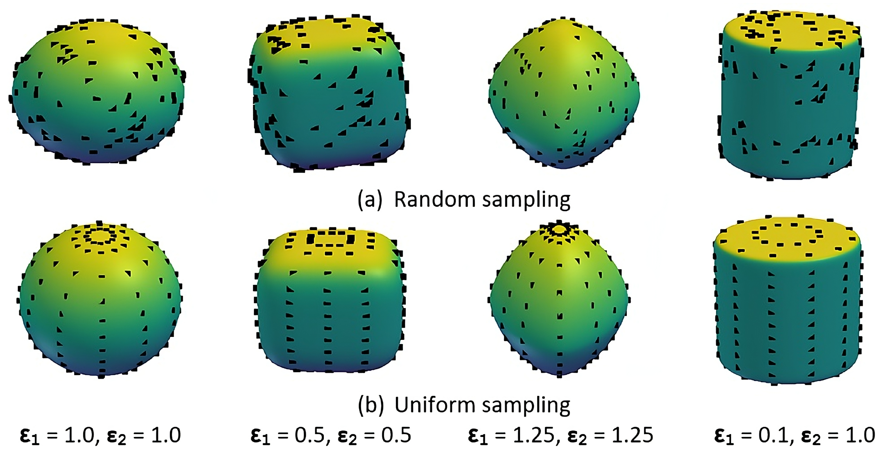
In previous superquadric-based models, the standard approach involved randomly sampling a fixed number of surface points—typically 200—from each primitive to approximate the expected loss. This stochastic process causes the sampled points to vary across training iterations, introducing fluctuations in the loss estimate. Although the variance of this estimate theoretically decreases with more samples, following Monte Carlo estimation principles, larger sample sizes significantly increase computational cost. In contrast to non-uniform methods, which cluster points in regions of high curvature or near poles, uniform sampling distributes points evenly across the surface, leading to more consistent approximations, reduced sampling bias, and improved accuracy in loss evaluation.
To improve sampling accuracy relative to non-uniform strategies [5], we evaluate two methods for generating surface points on superquadrics. The first method samples the parametric angles directly, following [5] and the equal-angle technique of [52]. Due to the non-linear mapping from parameter space to surface coordinates, this approach tends to cluster samples near poles and regions of high curvature, resulting in uneven coverage. The second method, adopted in our framework, samples points uniformly in parameter space and maps them to the surface using an inverse shape transformation that compensates for local density variations, thereby achieving a more balanced spatial distribution.
Comparing these two approaches highlights the impact of sampling uniformity on shape approximation. Non-uniform parameter-space sampling tends to over-represent flatter regions while under-sampling high-curvature zones, biasing the loss and impairing training stability. In contrast, the uniform surface-mapped sampling ensures equal contribution of all surface regions to the loss, yielding more stable optimization and higher-fidelity reconstruction. Empirically, this uniform sampling results in smoother convergence and better preservation of fine geometric details, particularly for superquadrics with extreme exponents that produce sharp edges or pinched regions.
Formally, in our implementation, surface sampling is parameterized using uniformly distributed angles , where and . Surface points computed via Equation (1) yield approximately uniform coverage across the superquadric surface, providing both a stable and computationally efficient sampling scheme for training.
Figure 6.
Comparison of sampling strategies for superquadrics. The proposed uniform surface-mapped approach produces a more even spatial distribution of points than the conventional random sampling method, leading to improved balance between the point cloud–to–primitive and primitive–to–point cloud loss components.
6.2. Overlapping Loss
Beyond minimizing reconstruction error between the input and predicted shapes, it is equally important to address the issue of overlapping between primitives. Excessive overlap introduces redundancy, reduces segmentation clarity, and hinders interpretability in downstream tasks such as robotic manipulation or physical simulation.
To explicitly mitigate this effect, we introduce an overlapping loss term that penalizes spatial intersections between primitives. The objective is to ensure that each primitive exclusively represents its own spatial region of the object and that surface points belonging to one primitive do not fall inside the geometry of any other.
The overlapping loss is computed by iterating over each primitive and testing whether its sampled surface points intersect with any other primitive. This process quantifies the degree of spatial redundancy among primitives. Formally, the total overlapping loss is defined as:
Here, M denotes the total number of primitives, K the number of sampled surface points per primitive, and a binary indicator function defined as:
In this definition, represents the k-th sampled surface point of the i-th primitive, and is the implicit inside–outside function (Equation (1)) evaluated for another primitive . If for any , the point is considered overlapping.
Unlike distance-based losses, this formulation directly counts the number of surface points from one primitive that intrude into others. Penalizing such intersections promotes spatial exclusivity, resulting in distinct and non-redundant partitions of the object’s geometry.
Revisiting Equation (9), which measures the fit between the predicted primitives and the input point cloud, it becomes evident that this formulation alone does not penalize overlaps among primitives. Consequently, multiple primitives may compete to represent the same surface regions, introducing ambiguity and reducing segmentation precision.
Incorporating the overlapping loss from Equation (12) introduces a complementary constraint that enforces exclusivity among primitives. This addition systematically discourages shared spatial regions and improves both the structural integrity and interpretability of the learned decomposition. In practice, it leads to cleaner segmentations and reduced redundancy, as demonstrated in the experimental results.
7. Experimental Evaluation
All experiments employ the Kaiming uniform weight initialization [41] to preserve gradient stability throughout training. This initialization maintains consistent activation variance across layers, preventing gradient explosion or vanishing. Combined with a cyclic learning rate scheduler [45], this configuration has been shown to enhance convergence speed and robustness in superquadric-based decomposition tasks [6]. We adopt the same setup to ensure reproducibility and stable optimization in our experiments.
We first analyze the impact of different sampling strategies on the stability and accuracy of loss estimation. The first strategy, originally employed by Paschalidou et al. [5], samples 200 points per primitive by randomly selecting angular parameters and , which define the surface coordinates of the superquadric.
The second strategy implements a uniform surface sampling method based on Pilu and Levialdi [52]. Instead of random selection, and are uniformly distributed and mapped to the superquadric surface via the parametric formulation (Equation (1)), yielding a more homogeneous spatial distribution of surface points.
For both strategies, we uniformly generate 200 surface points per primitive and compare them against a ground truth point cloud of 1000 points per object. The evaluation focuses on the effect of sampling uniformity on shape approximation accuracy, measured using our Structural Accuracy and Primitive Accuracy metrics, as well as the stability of training convergence.
Next, we evaluate the impact of the proposed overlapping loss in mitigating inter-primitive intersections. To isolate its effect, we compare our model against the baseline method [5] under identical sampling conditions. This controlled setup ensures that performance differences stem solely from the overlapping penalty rather than sampling variations.
Finally, we evaluate the combined impact of both improvements—the uniform sampling strategy and the overlapping loss—against the baseline [5]. This joint evaluation highlights the complementary nature of the two enhancements: while uniform sampling improves the accuracy and stability of loss estimation, the overlapping loss enforces spatial exclusivity, together leading to more coherent and interpretable decompositions.
7.1. Evaluation Metrics
Traditional reconstruction measures such as the Chamfer Distance (CD) and Earth Mover’s Distance (EMD) quantify point-level similarity between reconstructed and ground-truth shapes. However, these global distance metrics overlook structural and semantic relationships among primitives, offering limited insight into how well a model captures part-level geometry or inter-primitive consistency. Consequently, relying solely on these measures provides an incomplete understanding of primitive-based reconstruction performance.
To address this limitation, we introduce a novel evaluation framework that extends beyond surface-based metrics toward structure-aware assessment. Building upon our prior work [6], this framework incorporates three new complementary metrics—Primitive Accuracy (PA), Structural Accuracy (SA), and Overlapping Percentage (OP)—that collectively measure reconstruction quality from multiple perspectives. Primitive Accuracy directly quantifies the correspondence between predicted and ground-truth primitives, enabling the first objective evaluation of part-level geometric correctness. Structural Accuracy evaluates the global alignment and fidelity of the composed shape, while Overlapping Percentage measures redundancy and spatial coherence between adjacent primitives.
This design represents a conceptual advancement in evaluating interpretable 3D reconstruction. By shifting from point-based distances to primitive- and structure-aware metrics, our approach enables fairer, more interpretable, and reproducible comparisons between primitive-based models. It provides an essential foundation for future benchmarking efforts, promoting transparency and consistency in assessing primitive-based shape decomposition.
Structural Accuracy
Structural Accuracy quantifies how well the output primitives capture the structure of the input point cloud. Specifically, it measures the number of input points that are effectively represented by the predicted primitives, with higher values indicating better shape coverage.
Let N denote the total number of input points, and let represent the subset of points from the input that are covered by the generated primitives. Structural Accuracy (SA) is then defined as:
A higher Structural Accuracy value reflects a better correspondence between the predicted primitives and the true structure of the object, indicating the model’s effectiveness in representing the overall input geometry.
Primitive Accuracy
This metric evaluates how well each primitive aligns with the input point cloud while maintaining geometric consistency and meaningful segmentation. It measures the degree to which a primitive conforms to the shape and spatial distribution of its corresponding region in the input data.
In addition to alignment, the metric accounts for over spanning, which occurs when a primitive extends beyond its intended region and covers areas that do not belong to the target structure. A higher Primitive Accuracy score reflects both tighter geometric alignment and reduced over spanning, indicating that the predicted primitives effectively capture distinct and meaningful shape components.
The computation of Primitive Accuracy proceeds in five steps, as detailed below.
Step 1: Compute Radial Distances for Input Points To quantify geometric alignment, we compute the radial distance of each input point within the -plane. This projection-based measure simplifies the analysis by capturing the lateral spread of the shape while reducing sensitivity to vertical variations along the z-axis.
This formulation assumes a consistent orientation of the input object, where the -plane aligns with the object’s primary structural plane. Under this assumption, measuring radial distance from the origin is reasonable, as the origin serves as a reference point representing the object’s center. In more general cases, the metric can be adapted to each primitive’s local coordinate frame or center to accommodate arbitrary orientations.
Step 2: Filter Radial Distances Using Inside Mask The inside mask is defined as a binary indicator function that specifies whether each input point lies within the volume of a given primitive. This mask is used to filter the computed radial distances, ensuring that only points enclosed by the primitive contribute to the subsequent calculations.
Step 3: Estimate Mean Radial Distance (MRD) The mean radial distance (MRD) for each primitive is defined as the average two-dimensional radial distance of the input points enclosed by that primitive. The MRD serves as an indicator of the spatial extent of the region of the input point cloud represented by the primitive.
A significantly high MRD value may indicate a mismatch between the geometry of the input region and the superquadric form used to approximate it. For example, when the input resembles a toroidal shape (i.e., a structure with a central void), the model may assign a large MRD value to a primitive attempting to fit the outer ring. Because superquadrics cannot represent hollow structures like a torus, this leads to inaccurate modeling. Therefore, the MRD can serve as a diagnostic indicator for detecting such geometric mismatches and potential failure cases.
Step 4: Identify Geometric Mismatches Using Mean Radial Distance (MRD) Because our model is constrained to predict superquadrics—solid, closed surfaces—it cannot represent complex topologies such as toroidal shapes or objects containing substantial internal voids. To address this limitation without altering the model architecture, we introduce a diagnostic method that identifies when a predicted primitive is likely mismatched with the underlying input geometry. Specifically, the MRD computed from input points assigned to each primitive serves as a heuristic indicator of geometric mismatch. A high MRD value indicates that the primitive attempts to span an extended or disconnected region—behavior that is atypical for valid superquadric fitting. A mismatch detection function is defined to compare the MRD value against a predefined threshold. The proportion of primitives exceeding this threshold is then computed across the batch. This diagnostic is not used during training; instead, it serves as a post-hoc evaluation tool to reveal limitations in the model’s representational capacity and to identify cases where the predicted output fails to accurately capture the input geometry.
In practice, an MRD threshold of 0.05 (normalized by object scale) is used, which empirically separates valid from mismatched primitives across object categories.
Step 5: Calculate Primitive Accuracy The objective of this step is to compute a metric that quantifies how accurately each predicted primitive represents the input point cloud, capturing both geometric alignment and structural reliability.
Primitive Accuracy is defined as a weighted combination of two complementary components:
- Fit quality — the average geometric fit score of each primitive relative to its associated region in the input point cloud. Higher values indicate closer alignment, whereas overspanning leads to lower scores.
- Corrected Precision — the proportion of predicted primitives that are valid fits, i.e., not identified as mismatched shapes (such as those attempting to model toroidal or hollow structures). This value is computed using the mismatch detection method described in Step 4, where primitives with excessively high mean radial distance (MRD) values are flagged as invalid.
- A weighting factor is applied to balance geometric accuracy and structural correctness between the two terms.
The final Primitive Accuracy score is computed as a weighted sum of the fit quality and corrected precision terms, jointly reflecting geometric alignment and topological validity. By integrating these two components, Primitive Accuracy provides a comprehensive measure of each primitive’s performance in both surface fitting and structural interpretation.
Overlapping Percentage
In this paper, we introduce the Overlapping Percentage as a new metric to quantify the degree of spatial overlap between primitives during segmentation. Overlap occurs when points are simultaneously assigned to multiple primitives, indicating regions where segmentation boundaries are ambiguous or poorly defined. This metric is particularly useful for evaluating segmentation quality, since a high overlap value typically indicates low boundary precision and poor part separation.
The sensitivity of this metric may also depend on the primitive representation—such as pixel-wise masks, bounding boxes, or higher-level feature encodings—which affects how overlap is detected and interpreted. For instance, fine-grained representations such as masks can highlight subtle overlaps, whereas coarser representations such as bounding boxes may obscure them.
To compute the Overlapping Percentage, we first determine the number of points that are shared across different primitives. This count is then normalized by the total number of sampled surface points across all primitives, and the result is expressed as a percentage. Formally, the metric is defined as:
To compute the set of overlapping points, each surface point sampled from one primitive is tested against all other primitives using their implicit superquadric equations. The overlap condition for each sampled point is defined as:
The total number of overlapping points is obtained by summing over all sampled points and counting those that lie within at least one other primitive:

Table 2.
Indicator and evaluation functions used for geometric analysis and segmentation evaluation.
Table 2.
Indicator and evaluation functions used for geometric analysis and segmentation evaluation.
| Function | Definition |
|---|---|
| Overlap indicator: equals 1 if point k belonging to lies inside primitive j , and 0 otherwise. | |
| Returns 1 if the point lies inside primitive i (after transformation to its local coordinate frame), and 0 otherwise. | |
| Returns 1 if the i-th primitive exceeds the mean radial distance (MRD) threshold, indicating a geometric mismatch. | |
| Percentage of predicted primitives that are not identified as mismatched. | |
| Geometric fit score of primitives based on the average surface alignment with the input point cloud. | |
| Weighted combination of and , measuring both geometric and structural quality. | |
| Ratio of mismatched primitives to the total number of predicted primitives. |
7.2. Experiments
We now present our experimental results obtained using the ShapeNet dataset [53]. For consistency, we employ the official implementation of the baseline method described in [5].
Experiments are conducted on three representative object categories: chairs, airplanes, and tables. For each category, we select 20 samples, following the common practice in prior unsupervised shape decomposition studies [5,22]. Although the sample size may appear limited, this choice reflects the high computational cost associated with training and evaluation. Each object is represented using a fixed number of 20 superquadrics, ensuring consistency across all categories. This configuration offers a balanced trade-off between representational expressiveness and computational efficiency. In the experiments and tables, we refer to our previous model [6] as Eltaher for brevity.
All experiments are performed on a single NVIDIA RTX 3090 GPU, with each training session requiring approximately six hours to complete. We focus on the superquadric-based family of models [5,6], as they share a common implicit parametric structure and unsupervised optimization framework, ensuring methodological consistency and fair comparison.
Regarding evaluation metrics, conventional surface-based distances such as Chamfer Distance (CD) or Earth Mover’s Distance (EMD) are not used, as they primarily measure geometric proximity rather than structural fidelity. In the context of primitive-based shape abstraction, such metrics fail to capture essential factors like inter-primitive overlap, mismatched part assignments, or structural validity. Instead, we employ the proposed metrics—Structural Accuracy and Primitive Accuracy—which offer a more interpretable and task-relevant assessment of how well each predicted primitive represents the input geometry while preserving structural coherence.
Experiment 1: Comparison of Sampling Strategies
This experiment analyzes the effect of the traditional and proposed sampling strategies on the performance of two superquadric-based methods: the baseline method [5] and the Eltaher method [6]. The results in Table 3 indicate that the proposed uniform sampling strategy improves both Primitive Accuracy and Corrected Precision, particularly for the Eltaher method, while maintaining comparable performance in Overlapping Percentage and Structural Accuracy.
For the baseline method, switching from the traditional to the proposed sampling strategy yields a slight improvement in Primitive Accuracy (from an average of 0.036 to 0.058), accompanied by a minor decline in Structural Accuracy (from 0.90 to 0.88). This trade-off can be attributed to the following factors:
- Primitive Accuracy Improvement: The proposed sampling strategy enables a more uniform and representative distribution of surface points, reducing segmentation errors and improving the reconstruction accuracy of individual superquadrics.
- Structural Accuracy Decline: The moderate decrease in Structural Accuracy indicates that, although the new sampling promotes more coherent segmentation, it may marginally reduce the tightness of fit between reconstructed primitives and the input point cloud.
- Overlapping Percentage Consistency: The overlapping percentage remains constant at 0.99, indicating that the baseline method continues to exhibit excessive primitive intersections, reflecting an absence of explicit constraints to enforce non-overlapping segmentation.
In Table 3, the Corrected Precision value of 0.00 observed for the baseline method may appear anomalous. This outcome occurs when the baseline model attempts to decompose objects containing topological holes (e.g., mugs with handles). Because superquadrics represent closed surfaces by definition, the decomposition cannot accurately capture such open or hollow structures. Consequently, nearly all predicted primitives fail to correspond to the target shape components, resulting in a Corrected Precision value of zero. This observation underscores the limitation of relying solely on Structural Accuracy or distance-based metrics, as these can be misleading when evaluating complex or topologically nontrivial shapes. The Corrected Precision metric was thus introduced to provide a more reliable assessment of primitive correctness in such challenging scenarios.
For the Eltaher method, the uniform sampling strategy yields a distinct improvement in Primitive Accuracy, increasing from an average of 0.59 to 0.65. In contrast, Structural Accuracy shows a modest decrease from 0.90 to 0.84. These variations are primarily explained by the following factors:
- Improved Primitive Accuracy: The Eltaher method demonstrates greater improvement under the uniform sampling strategy owing to its refined primitive fitting mechanism. The refined point selection enables the model to align predicted superquadrics more accurately with the geometric structure of the object.
- Moderate Structural Accuracy Reduction: Although individual primitives more accurately represent local shape components, the overall reconstruction can exhibit minor gaps or misalignments between adjacent parts, slightly reducing overall structural coherence.
- Stable Overlapping Performance: The Eltaher method consistently maintains low overlapping percentages (ranging from 0.15 to 0.28) due to its integrated spatial separation constraints. The slight increase observed with uniform sampling (maximum value rising from 0.20 to 0.28) likely indicates improved geometric coverage rather than deviation from strict non-overlap.
Summary
- Baseline Method: The uniform sampling strategy yields a moderate increase in primitive accuracy (from 0.036 to 0.058 on average). However, the overlapping percentage remains substantially high (unchanged at 0.99), and structural accuracy shows a minor decrease (from 0.90 to 0.88), as reported in Table 3.
- Eltaher Method: The uniform sampling strategy produces a notable improvement in primitive accuracy (from 0.59 to 0.65 on average), accompanied by a slight reduction in structural accuracy (from 0.90 to 0.84). Nevertheless, the method maintains a substantially lower overlapping percentage (ranging from 0.20 to 0.28) compared with the baseline approach.
- Structural vs. Primitive Accuracy Trade-off: The results indicate that improvements in primitive accuracy are often accompanied by slight reductions in structural accuracy. This observation suggests that improved part-level fitting and segmentation may occur at the expense of global shape coherence.
Experiment 2: Effect of the Number of Sampled Points per Primitive
This experiment investigates how varying the number of sampled points per primitive (200 and 100) affects the performance of the baseline method [5] and the Eltaher method [6], evaluated under both the old and uniform sampling strategies. The results for all configurations are summarized in Table 4, based on evaluations conducted on the mug category from the ShapeNet dataset. The evaluation metrics considered are: Overlapping Percentage, Structural Accuracy, Primitive Accuracy, and Corrected Precision.
For the baseline method, the Overlapping Percentage is constant at 0.99 across all configurations. This consistency indicates that the baseline method exhibits persistent excessive intersection among primitives, independent of the sampling strategy or point count. This observation supports the conclusion drawn from Table 4 that the method lacks explicit mechanisms to penalize overlap during reconstruction.
Structural Accuracy is stable at 0.90 across all conditions, suggesting that the baseline method’s shape-fitting performance is largely unaffected by changes in sampling density. However, Primitive Accuracy increases appreciably with the uniform sampling strategy:
- With 200 points per primitive, Primitive Accuracy increases from 0.036 (old sampling) to 0.077 (uniform sampling).
- With 100 sampled points per primitive, Primitive Accuracy further increases to 0.083.
This improvement suggests that the uniform sampling strategy yields more informative point distributions, facilitating more accurate segmentation of individual primitives. However, Corrected Precision shows a slight decrease from 0.10 (with 200 points) to 0.050 (with 100 points), indicating that reduced point density can impair geometric precision in certain cases.
For the Eltaher method, the Overlapping Percentage is considerably lower than that of the baseline approach. The Overlapping Percentage increases slightly when fewer points are used:
- Under the previous sampling strategy, overlapping increases from 0.20 (with 200 points) to 0.28 (with 100 points).
- Under the uniform sampling strategy, the overlapping value increases slightly from 0.20 to 0.24.
These small increases suggest that although the Eltaher method effectively constrains overlaps through its architectural design, lower sampling densities can introduce minor geometric instability. Structural Accuracy shows a slight decrease from 0.90 (under the previous sampling strategy) to 0.84 (under the uniform sampling strategy), consistent with the trends observed in Experiment 1. This trade-off likely reflects a shift in optimization focus toward enhanced segmentation quality at the expense of precise global alignment.
Primitive Accuracy improves under the uniform sampling strategy:
- Increasing from 0.60 to 0.70 when using 200 sampled points per primitive.
- Increasing from 0.61 to 0.71 when using 100 sampled points per primitive.
These results indicate that the uniform sampling strategy enhances segmentation quality even with reduced point density and aligns effectively with the Eltaher method’s primitive-fitting design. Corrected Precision remains constant at 1.00 across all configurations, underscoring the robustness of the Eltaher method’s segmentation performance.
The key findings from this experiment can be summarized as follows:
- Baseline Method: The uniform sampling strategy improves Primitive Accuracy, but the Overlapping Percentage remains high, and Structural Accuracy is largely unaffected by the number of sampled points (see Table 4).
- Eltaher Method: The uniform sampling strategy improves Primitive Accuracy while maintaining relatively low Overlapping Percentages, demonstrating superior segmentation quality across varying sampling densities.
- Effect of Points per Primitive: Using 100 points per primitive often yields slightly higher Primitive Accuracy, whereas 200 points produce lower Overlapping Percentages, making the latter configuration preferable when aiming to reduce segmentation redundancy.
Figure 7 provides qualitative support for these findings, illustrating segmentation coherence across sampling configurations. Segmentations generated using the uniform sampling strategy with 200 points appear more coherent and better aligned with object parts, particularly in challenging regions such as the mug handle. The Eltaher method exhibits the most visually consistent performance, characterized by minimal fragmentation and high part-level fidelity.
Overall, the findings support the conclusion that combining the uniform sampling strategy with a higher point density achieves an optimal balance between precise primitive segmentation and minimal inter-primitive overlap, particularly in the Eltaher method.
Experiment 3: Effect of Overlapping Loss on Baseline and Eltaher Methods
This experiment examines the effect of introducing an overlapping loss to both the baseline method [5] and the Eltaher method [6]. The evaluation results, summarized in Table 5, are reported in terms of Overlapping Percentage, Structural Accuracy, Primitive Accuracy, and Corrected Precision. All values represent averages computed over ten independent runs on the mug category of the ShapeNet dataset.
For the baseline method, incorporating the overlapping loss does not reduce the Overlapping Percentage, which remains constant at 0.99. This finding indicates a persistent tendency toward excessive primitive overlap, suggesting that overlapping loss alone is insufficient to mitigate this limitation. Nonetheless, small improvements are observed in both Structural and Primitive Accuracy. Structural Accuracy increases from 0.88 to 0.89, while Primitive Accuracy rises from 0.0365 to 0.0636. However, Corrected Precision remains unchanged at 0.10, indicating that segmentation precision does not improve under this configuration.
In contrast, the Eltaher method exhibits greater performance improvements. The Overlapping Percentage decreases from 0.24 to 0.20, while Primitive Accuracy rises from 0.60 to 0.64. These results suggest that the overlapping loss effectively mitigates over-segmentation and promotes improved geometric alignment. A slight decrease in Structural Accuracy is noted (from 0.93 to 0.91), which may reflect a limited trade-off in fitting flexibility. However, Corrected Precision remains constant at 1.00 in both cases, indicating high consistency and reliability in the segmentation output.
The key findings from this experiment can be summarized as follows:
- For the baseline method, the overlapping loss yields minor improvements in accuracy metrics but does not reduce overlap. Corrected Precision remains low, indicating limited practical benefit.
- For the Eltaher method, the overlapping loss leads to enhanced primitive separation and accuracy, with only a minimal reduction in Structural Accuracy. Corrected Precision remains constant at 1.00, demonstrating stable segmentation performance.
- Overall, the overlapping loss demonstrates higher effectiveness in enhancing segmentation quality when applied to more expressive architectures such as the Eltaher method, while offering limited improvement for the baseline approach.
Experiment 4: Comparison Across Object Categories
This experiment evaluates the performance of the proposed model against the baseline method [5] and the Eltaher method [6] on three object categories from the ShapeNet dataset: chairs, airplanes, and tables. Table 6 presents the results for each method in terms of Overlapping Percentage, Structural Accuracy, Primitive Accuracy, and Corrected Precision, averaged over twenty input shapes per category.
Chair category. Chairs exhibit thin structures and complex geometries that pose significant challenges for segmentation models. The baseline method shows limited performance, exhibiting a high overlapping percentage (0.89) and the lowest structural accuracy (0.81), indicating substantial primitive intersection and weak overall shape representation. The Eltaher method reduces overlap to 0.30, leading to a marked improvement in structural accuracy (0.94), although primitive accuracy remains limited at 0.52. The proposed model achieves further gains, with reduced overlap (0.22), higher primitive accuracy (0.61), and perfect corrected precision (1.00), suggesting improved segmentation fidelity and more precise primitive placement.
Airplane category. The streamlined shapes and symmetrical components of airplanes pose significant challenges for accurate geometric decomposition. The baseline method exhibits an overlapping percentage of 0.64 and a lower primitive accuracy (0.47), reflecting imprecise segmentation of major structural components. The Eltaher method improves primitive accuracy to 0.63 while reducing the overlapping percentage to 0.40. The proposed model further increases primitive accuracy to 0.69, exhibiting a slightly higher overlap (0.45) than the Eltaher method, along with a modest reduction in structural accuracy (from 0.95 to 0.90). Both methods maintain a corrected precision of 1.00, indicating accurate and consistent boundary delineation.
Table category. Tables generally feature flat surfaces and thin supports, which pose challenges for achieving accurate and clean segmentation. The baseline method shows the weakest performance, with an overlapping percentage of 0.97 and the lowest primitive accuracy (0.44). The Eltaher method lowers overlap to 0.33 and attains a structural accuracy of 0.96, although primitive accuracy remains low at 0.43. The proposed model further reduces overlap to 0.24 and substantially improves primitive accuracy to 0.69. Corrected Precision attains a value of 1.00, and despite a slight decrease in Structural Accuracy (from 0.96 to 0.90), the results indicate an overall improvement in decomposition quality.
Qualitative validation.Figure 8 and Figure 9 provide qualitative validation and visual support for these observations. Compared with the baseline and the Eltaher method, the proposed model produces cleaner and more compact segmentations. Primitive boundaries align more consistently with the underlying object geometry, avoiding the oversized and redundant primitives observed in the baseline and improving upon the moderate overlap present in the Eltaher method.
The key findings from this qualitative analysis can be summarized as follows:
- The proposed model consistently reduces the overlapping percentage across all categories, particularly for complex shapes such as chairs and tables.
- Primitive accuracy is higher in all cases, indicating improved geometric correspondence and more accurate primitive assignment.
- Corrected Precision remains constant at 1.00 across all categories, demonstrating high consistency and reliability in primitive placement.
- Structural Accuracy exhibits minor variation, reflecting trade-offs between precise surface fitting and enhanced segmentation compactness.
Experiment 5: Visual Comparison of Segmentation Quality
This experiment presents a qualitative analysis of segmentation quality across multiple object categories, as illustrated in Figure 10. The comparison highlights the differences among the proposed method, the baseline approach [5], and the Eltaher method [6], with a particular focus on challenging categories such as chairs, tables, mugs, and bags.
Chair category. Chairs are structurally complex objects, characterized by thin components and intricate interconnections. The baseline method exhibits excessive overlap, resulting in primitive extensions that obscure the boundaries between arms, seats, and backrests. The Eltaher method improves segmentation by reducing overlap and enhancing part-level separation. However, primitive misalignments persist, particularly around the base and backrest regions. The proposed method produces clearer boundaries and more accurately aligned primitives, particularly in the arm and leg regions. This leads to a more coherent and perceptually natural decomposition.
Table category. Tables present segmentation challenges due to their flat top surfaces and thin supporting structures. The baseline method exhibits limited differentiation between components, resulting in redundant and oversized primitives. The Eltaher method reduces overlap and enhances component separation, although certain structural inconsistencies persist. The proposed method yields the cleanest segmentation, effectively separating the tabletop from the supporting legs with minimal overlap. The resulting primitive layout produces a more accurate and compact representation of the overall structure.
Mug and bag categories. These categories are characterized by curved geometries and fine structural details. The baseline method exhibits significant primitive overlap, resulting in misalignment and poor coverage of distinct components, such as the handle of a mug or the folds of a bag. The Eltaher method enhances structural coherence but still exhibits occasional primitive misplacement. In contrast, the proposed method achieves precise segmentation, accurately capturing the mug’s handle and following the natural contours of the bag with minimal redundancy.
Visual evidence.Figure 10 illustrates that the proposed method consistently yields the most compact and clean primitive representations. The baseline method exhibits severe over-segmentation, while the previous approach achieves moderate improvements. In contrast, the proposed model demonstrates the highest visual quality, with superior primitive alignment and structural consistency.
The key findings from this visual comparison can be summarized as follows:
- The proposed model outperforms both the baseline and the Eltaher method in visual segmentation quality, particularly for geometrically complex shapes.
- Primitive alignment and boundary clarity are substantially improved, especially in detailed regions such as handles and structural joints.
- The visual results reinforce the quantitative improvements, confirming the robustness and generalization capability of the proposed method across diverse object categories.
8. Conclusions and Future Work
This study presented a set of methodological and conceptual advancements for superquadric-based frameworks in three-dimensional (3D) shape representation. A central contribution lies in the formulation of an overlapping loss function that mitigates a key limitation of prior methods—excessive intersection among primitives. Such overlaps reduce segmentation interpretability and geometric clarity, introducing redundant surface regions that degrade both visual quality and utility for downstream applications such as robotic manipulation or physical simulation. The proposed overlapping loss penalizes spatial intrusions between primitives, promoting exclusive spatial partitioning and resulting in more coherent, interpretable decompositions.
To enhance training stability, a uniform surface sampling strategy was introduced to ensure even point distribution across primitive surfaces. Unlike random sampling, which often yields uneven coverage, the uniform approach produces statistically balanced sampling, improving optimization behavior and reconstruction fidelity.
Beyond architectural and training refinements, this work introduces a novel, structure-aware evaluation framework that advances the methodology for assessing primitive-based 3D reconstruction. This framework integrates three complementary metrics—Primitive Accuracy, Structural Accuracy, and Overlapping Percentage—which collectively capture both local geometric fidelity and global structural consistency. By moving beyond traditional point-based metrics such as Chamfer Distance and Earth Mover’s Distance, this framework establishes a new standard for quantitative, interpretable, and reproducible evaluation in primitive-based modeling.
Experimental results across multiple 3D object categories demonstrate that the proposed enhancements yield more accurate, compact, and semantically coherent decompositions. The approach not only improves reconstruction quality but also provides a principled foundation for future benchmarking and comparative studies in interpretable 3D representation learning.
Future work may extend this framework along several promising directions that span both methodological and application-oriented domains. In robotics, interpretable primitive-based decompositions could improve grasp planning, collision-free manipulation, and object interaction [54,55], particularly when extended to noisy or partial sensor data. Robustness and generalization should also be investigated across larger and more diverse datasets, such as ShapeNet [53], ModelNet [56], or real-world scans, to evaluate resilience under occlusion and noise.
At the representation level, hybrid modeling constitutes an important avenue for exploration. Combining superquadric primitives with neural implicit fields such as DeepSDF [21] or NeRF [23], as well as mesh-based methods [57], may balance interpretability and expressiveness, enabling detailed yet structured reconstructions. Extending the primitive family to include deformable or parametric variants—such as tapering, bending, or localized deformations—may further enhance flexibility in representing organic and highly curved objects.
From an application perspective, primitive-based modeling naturally aligns with computer-aided design (CAD) and shape-editing tasks. Its parametric and interpretable nature lends itself to interactive or generative design workflows where human input guides the decomposition process [58,59]. Finally, the proposed evaluation metrics open opportunities for standardized benchmarking. Future research could extend these metrics into community-adopted protocols, enabling consistent, transparent comparison across primitive-based models and fostering progress toward interpretable unsupervised 3D representation learning.
Looking forward, these directions indicate that primitive-based modeling can continue to evolve at the intersection of geometry, learning, and application. By connecting analytic decomposition more closely with robotic perception, interactive design, and standardized evaluation, the framework established in this work lays the foundation for scalable, interpretable, and semantically meaningful 3D shape understanding.
Author Contributions
Conceptualization, M.E.; methodology, M.E.; software, M.E.; validation, M.E.; formal analysis, M.E.; investigation, M.E.; data curation, M.E.; writing—original draft preparation, M.E.; visualization, M.E.; writing—review and editing, M.B.; supervision, M.B.; project administration, M.B.; funding acquisition, M.B. All authors have read and agreed to the published version of the manuscript.
Funding
This work was supported by the German Aerospace Center (DLR) under grant number . The APC was funded by the same source.
Institutional Review Board Statement
Not applicable. This study does not involve humans or animals.
Informed Consent Statement
Not applicable.
Data Availability Statement
The datasets used in this study are publicly available from the ShapeNet repository [53]. Additional figures and code are available upon reasonable request from the corresponding author.
Acknowledgments
The authors would like to thank the German Aerospace Center (DLR) for funding support.
Conflicts of Interest
The authors declare no conflict of interest.
References
- Gupta, S.; Johnson, J.; Savarese, S.; Fei-Fei, L. Aligning 3D CAD models with RGB-D scans. In Proceedings of the Proceedings of the IEEE Conference on Computer Vision and Pattern Recognition (CVPR), 2015, pp. 6239–6247.
- Qi, C.R.; Su, H.; Mo, K.; Guibas, L.J. Pointnet: Deep learning on point sets for 3d classification and segmentation. In Proceedings of the Proceedings of the IEEE conference on computer vision and pattern recognition, 2017, pp. 652–660.
- Wang, B. Dynamic content monitoring and exploration using vector spaces. In Proceedings of the Proceedings of the 42nd International ACM SIGIR Conference on Research and Development in Information Retrieval, 2019, pp. 1444–1444.
- Barr, A.H. Superquadrics and Angle-Preserving Transformations. IEEE Comput. Graph. Appl. 1981, 1, 11–23. https://doi.org/10.1109/MCG.1981.1673798.
- Paschalidou, G.; Bogo, F.; Geiger, A.; Matusik, W. Superquadrics for 3D Shape Representation and Reconstruction. In Proceedings of the Proceedings of the IEEE Conference on Computer Vision and Pattern Recognition (CVPR), 2019, pp. 5035–5044.
- Eltaher, M.; Breuss, M. Unsupervised Description of 3D Shapes by Superquadrics Using Deep Learning. Computer Vision and Machine Intelligence 2023, pp. 95–107.
- Pentland, A.P. Perceptual Organization and the Representation of Natural Form. Artificial Intelligence 1986, 28, 293–331.
- Solina, F.; Bajcsy, R. Recovery of parametric models from range images: The case for superquadrics with global deformations. IEEE transactions on pattern analysis and machine intelligence 1990, 12, 131–147.
- Cao, J.; Liu, Y.; Chen, Z. Primitive-based 3D segmentation for CAD models. Computer-Aided Design 2011, 43, 1328–1338. https://doi.org/10.1016/j.cad.2011.06.013.
- Funkhouser, T.; Shilane, P. A survey of methods for detecting partial 3D shape similarity. Proceedings of the IEEE Conference on Computer Graphics and Applications 1997, 97, 40–47. https://doi.org/10.1109/38.626968.
- Roberts, L.G. Machine perception of three-dimensional solids. PhD thesis, Massachusetts Institute of Technology, 1963.
- Binford, I. Visual perception by computer. In Proceedings of the IEEE Conference of Systems and Control, 1971, pp. 32–43.
- Terzopoulos, D.; Witkin, A.; Kass, M. Constraints on Deformable Models: Recovering 3D Shape and Nonrigid Motion. Artificial Intelligence 1988, 36, 91–123.
- Grossmann, E. Fitting Superquadrics to Range Data: Improving Shape Recovery. Computer Vision, Graphics, and Image Processing 1987, 40, 277–291. https://doi.org/10.1016/0734-189X(87)90073-8.
- Smith, W.; Hancock, E.R. Recovering Superquadric Models from Range Data Using Optimization. Computer Vision and Image Understanding 1997, 65, 256–284. https://doi.org/10.1006/cviu.1996.0602.
- Leonardis, A.; Jaklič, A.; Solina, F. Superquadrics for Segmenting and Modeling Range Data. IEEE Transactions on Pattern Analysis and Machine Intelligence 1998, 20, 1229–1235. https://doi.org/10.1109/34.730560.
- Besl, P.J.; McKay, N.D. A Method for Registration of 3D Shapes. IEEE Transactions on Pattern Analysis and Machine Intelligence 1992, 14, 239–256.
- Jiang, Y.; Zakka, K.; Dellaert, F.; Fox, D.; Srinivasa, S. Synergies between Affordance and Geometry: Affordance-Guided 3D Shape Reconstruction. In Proceedings of the Proceedings of the IEEE/CVF International Conference on Computer Vision (ICCV), 2021, pp. 2090–2099.
- Wu, J.; Zhang, C.; Xue, T.; Freeman, W.T.; Tenenbaum, J.B. Modeling 3D shapes by reinforcement learning. In Proceedings of the Advances in Neural Information Processing Systems (NeurIPS), 2015, pp. 4097–4105.
- Paschalidou, D.; Gool, L.V.; Geiger, A. Learning unsupervised hierarchical part decomposition of 3d objects from a single rgb image. In Proceedings of the Proceedings of the IEEE/CVF Conference on Computer Vision and Pattern Recognition, 2020, pp. 1060–1070.
- Park, J.J.; Florence, P.; Straub, J.; Newcombe, R.; Lovegrove, S. DeepSDF: Learning Continuous Signed Distance Functions for Shape Representation. CVPR 2019.
- Mescheder, L.; Oechsle, M.; Niemeyer, M.; Nowozin, S.; Geiger, A. Occupancy Networks: Learning 3D Reconstruction in Function Space. In Proceedings of the Proceedings of the IEEE/CVF Conference on Computer Vision and Pattern Recognition (CVPR), 2019, pp. 4460–4470.
- Mildenhall, B.; Srinivasan, P.P.; Tancik, M.; Barron, J.T.; Ramamoorthi, R.; Ng, R. NeRF: Representing Scenes as Neural Radiance Fields for View Synthesis. Communications of the ACM 2021, 65, 99–106.
- Sitzmann, V.; Thies, J.; Zollhöfer, M.; Heide, F.; Nießner, M.; Wetzstein, G. Scene Representation Networks: Continuous 3D-Structure-Aware Neural Scene Representations. Advances in Neural Information Processing Systems (NeurIPS) 2019.
- Maturana, D.; Scherer, S. Voxnet: A 3d convolutional neural network for real-time object recognition. In Proceedings of the 2015 IEEE/RSJ International Conference on Intelligent Robots and Systems (IROS), 2015, pp. 922–928.
- Riegler, G.; Kaden, G.; Stojanovic, J.; Zoller, D.; Zhang, J.; Liu, X.; Wenzel, F. OctNet: Learning Deep 3D Representations at a High Computational Efficiency. In Proceedings of the Proceedings of the IEEE Conference on Computer Vision and Pattern Recognition (CVPR), 2017, pp. 5171–5180.
- Masci, J.; Boscaini, D.; Bronstein, M.; Vandergheynst, P. Geodesic convolutional neural networks on Riemannian manifolds. In Proceedings of the Proceedings of the IEEE International Conference on Computer Vision Workshops (ICCVW), 2015, pp. 37–45.
- Ranjan, A.; Bolkart, T.; Black, M.J.; Sanyal, S.; et al. Generating 3D faces using convolutional mesh autoencoders. In Proceedings of the ECCV, 2018, pp. 725–741.
- Landrieu, L.; Simonovsky, M. Large-Scale Point Cloud Semantic Segmentation with Superpoint Graphs. Proceedings of the IEEE Conference on Computer Vision and Pattern Recognition (CVPR) 2018, pp. 4558–4567.
- Tulsiani, S.; Su, H.; Guibas, L.J.; Efros, A.A.; Malik, J. Learning shape abstractions by assembling volumetric primitives. In Proceedings of the Proceedings of the IEEE Conference on Computer Vision and Pattern Recognition, 2017, pp. 2635–2643.
- Paschalidou, D.; Katharopoulos, A.; Geiger, A.; Fidler, S. Neural Parts: Learning expressive 3D shape abstractions with invertible neural networks. In Proceedings of the Proceedings of the IEEE/CVF Conference on Computer Vision and Pattern Recognition, 2021, pp. 3204–3215.
- Yang, K.; Chen, X. Unsupervised learning for cuboid shape abstraction. ACM Transactions on Graphics (TOG) 2021, 40, 1–13. https://doi.org/10.1145/3450626.3459873.
- Xu, X.; Guerrero, P.; Fisher, M.; Singh, S. Unsupervised 3D shape reconstruction by part regularization. In Proceedings of the Proceedings of the IEEE/CVF Conference on Computer Vision and Pattern Recognition (CVPR), 2023, pp. 827–836. https://doi.org/10.1109/cvpr52729.2023.00827.
- Yuldasheva, S.M. Unsupervised description of 3D shapes by superquadrics. In Computational Vision and Graphics; Springer, 2023; pp. 189–205. https://doi.org/10.1007/978-981-19-7867-8_9.
- Li, P.; Guo, J.; Li, H.; Beneš, B. SfmCAD: Unsupervised CAD reconstruction by learning structural and free-form primitives. In Proceedings of the Proceedings of the IEEE/CVF Conference on Computer Vision and Pattern Recognition (CVPR), 2024, pp. 447–456. https://doi.org/10.1109/cvpr52733.2024.00447.
- Li, J.; Wang, H.; Tan, J.; Zhang, J. Shared latent membership enables joint shape analysis and reconstruction. IEEE Transactions on Image Processing 2024, 33, 4312–4325. https://doi.org/10.1109/TIP.2024.3404234.
- Li, S.; Paschalidou, D.; Guibas, L. PASTA: Controllable part-aware shape generation. arXiv preprint arXiv:2407.13677 2024.
- Chen, X.; Cheng, Z. Learning 3D representations from procedural 3D data. arXiv preprint arXiv:2411.17467 2024.
- Kobsik, G.; Henkel, M.; He, Y.; Kroemer, O. Learning fine-to-coarse cuboid shape abstraction. arXiv preprint arXiv:2502.01855 2025.
- Ye, J.; He, Y.; Zhou, Y.; Zhu, Y.; Xu, K. PrimitiveAnything: Human-crafted 3D primitive abstraction with foundation models. arXiv preprint arXiv:2505.04622 2025.
- He, K.; Zhang, X.; Ren, S.; Sun, J. Delving deep into rectifiers: Surpassing human-level performance on imagenet classification. In Proceedings of the Proceedings of the IEEE international conference on computer vision, 2015, pp. 1026–1034.
- Wu, Z.; Song, S.; Khosla, A.; Yu, F.; Zhang, L.; Tang, X.; Xiao, J. 3D ShapeNets: A deep representation for volumetric shapes. In Proceedings of the Proceedings of the IEEE Conference on Computer Vision and Pattern Recognition (CVPR), 2015, pp. 1912–1920.
- Sharma, A.; Grau, O.; Fritz, M. VConv-DAE: Deep volumetric shape learning without object labels. In Proceedings of the Proceedings of the European Conference on Computer Vision (ECCV), 2016, pp. 236–250.
- Wang, Y.; Sun, Y.; Liu, Z.; Sarma, S.E.; Bronstein, M.M.; Solomon, J.M. VoxSegNet: Volumetric CNNs for semantic part segmentation of 3D shapes. In Proceedings of the Proceedings of the IEEE/CVF Conference on Computer Vision and Pattern Recognition (CVPR), 2018, pp. 856–865.
- Smith, L.N. Cyclical Learning Rates for Training Neural Networks. In Proceedings of the 2017 IEEE Winter Conference on Applications of Computer Vision (WACV), 2017, pp. 464–472.
- Livne, A.; Barnea, E.; Ben-Shahar, O. Superquadric Decomposition for Robust 3D Object Representation. IEEE Transactions on Pattern Analysis and Machine Intelligence 2020, 42, 1854–1867.
- Leonardis, A.; Solina, F. Superquadrics for Segmenting and Modeling Range Data. IEEE Transactions on Pattern Analysis and Machine Intelligence 1997, 19, 1289–1295. https://doi.org/10.1109/34.643875.
- Choy, C.B.; Xu, H.; Gwak, J.; Chen, J.; Savarese, S. 3D-R2N2: A Unified Approach for Single and Multi-view 3D Object Reconstruction. In Proceedings of the Proceedings of the European Conference on Computer Vision (ECCV), 2016, pp. 628–644.
- Shi, W.; Rajkumar, R. Point-gnn: Graph neural network for 3d object detection in a point cloud. In Proceedings of the Proceedings of the IEEE/CVF conference on computer vision and pattern recognition, 2020, pp. 1711–1719.
- Wu, B.; Liu, Y.; Lang, B.; Huang, L. DGCNN: Disordered graph convolutional neural network based on the Gaussian mixture model. Neurocomputing 2018, 321, 346–356.
- Vaskevicius, N.; Birk, A. Revisiting superquadric fitting: A numerically stable formulation. IEEE transactions on pattern analysis and machine intelligence 2017, 41, 220–233.
- Pilu, M.; Fisher, R.B. Equal-distance sampling of superellipse models. Technical Report DAI Research Paper No. 794, University of Edinburgh, Department of Artificial Intelligence, 1995.
- Chang, A.X.; Funkhouser, T.; Guibas, L.; Hanrahan, P.; Huang, Q.; Li, Z.; Savarese, S.; Savva, M.; Song, S.; Su, H.; et al. Shapenet: An information-rich 3d model repository. arXiv preprint arXiv:1512.03012 2015.
- Miller, A.T.; Allen, P.K. GraspIt!: A versatile simulator for robotic grasping. IEEE Robotics & Automation Magazine 2003, 11, 110–122.
- Tripathi, S.; Gupta, A.; Knoop, E.; Van Der Stappen, A.F.; Kragic, D. Superquadric representations for object perception and manipulation. In Proceedings of the 2020 IEEE International Conference on Robotics and Automation (ICRA). IEEE, 2020, pp. 6243–6250.
- Wu, Z.; Song, S.; Khosla, A.; Yu, F.; Zhang, L.; Tang, X.; Xiao, J. 3d shapenets: A deep representation for volumetric shapes. In Proceedings of the Proceedings of the IEEE conference on computer vision and pattern recognition, 2015, pp. 1912–1920.
- Kanazawa, A.; Tulsiani, S.; Efros, A.A.; Malik, J. Learning category-specific mesh reconstruction from image collections. In Proceedings of the Proceedings of the European Conference on Computer Vision (ECCV), 2018, pp. 371–386.
- Company, P.; Contero, M.; Piquer, A. A survey on parametric surfaces and their applications in CAD, graphics and engineering. Computer-Aided Design and Applications 2009, 6, 541–562.
- Attene, M.; Falcidieno, B.; Spagnuolo, M. Shape modeling by sketching: A review of sketch-based modeling systems. Computers & Graphics 2013, 37, 485–501.
Figure 1.
Results on the ShapeNet dataset. (First row) Input point clouds; (second row) outputs of the baseline method [5]. The baseline model exhibits high sensitivity to random initialization, often resulting in segmentation inconsistencies and excessive overlap between primitives. Such overlap can obscure fine geometric details and lead to suboptimal shape decomposition, highlighting the need for improved initialization strategies and overlap-aware optimization.
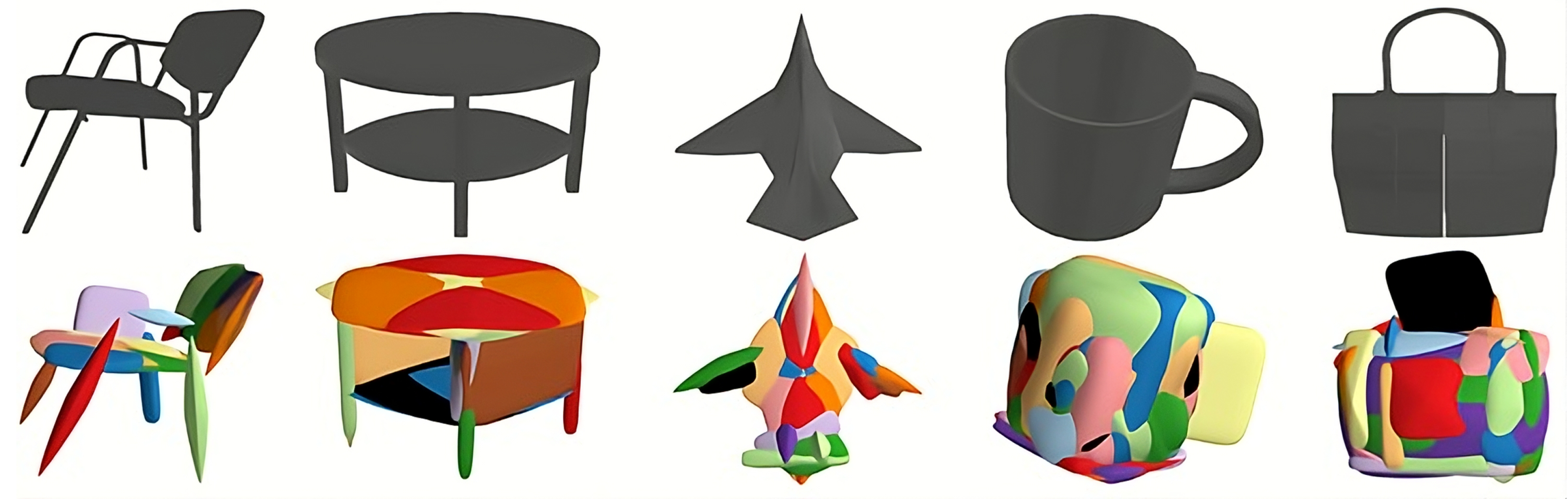
Figure 2.
Visualization of superquadrics generated with varying shape exponents and , while keeping the scale parameters , , and constant.
Figure 2.
Visualization of superquadrics generated with varying shape exponents and , while keeping the scale parameters , , and constant.
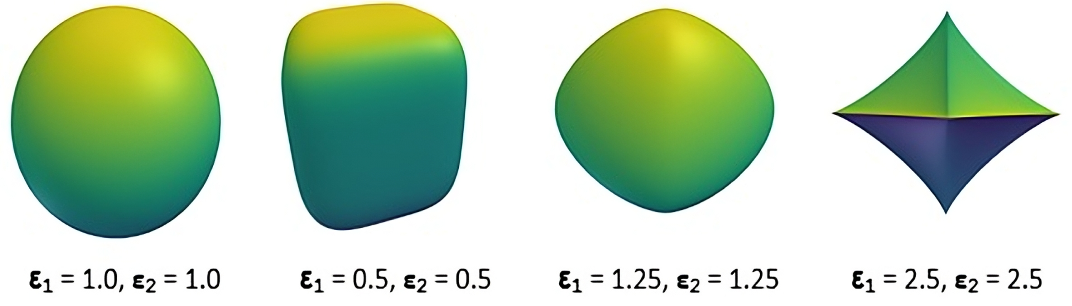
Figure 3.
Visualization of the geometric distance terms used in surface–point correspondence and loss computation. Left: The term represents the minimum distance from each sampled point on the surface of the i-th primitive (squares) to the set of input points in the point cloud (circles). Right: The term represents the minimum distance from each input point to the set of sampled surface points of the corresponding primitive.
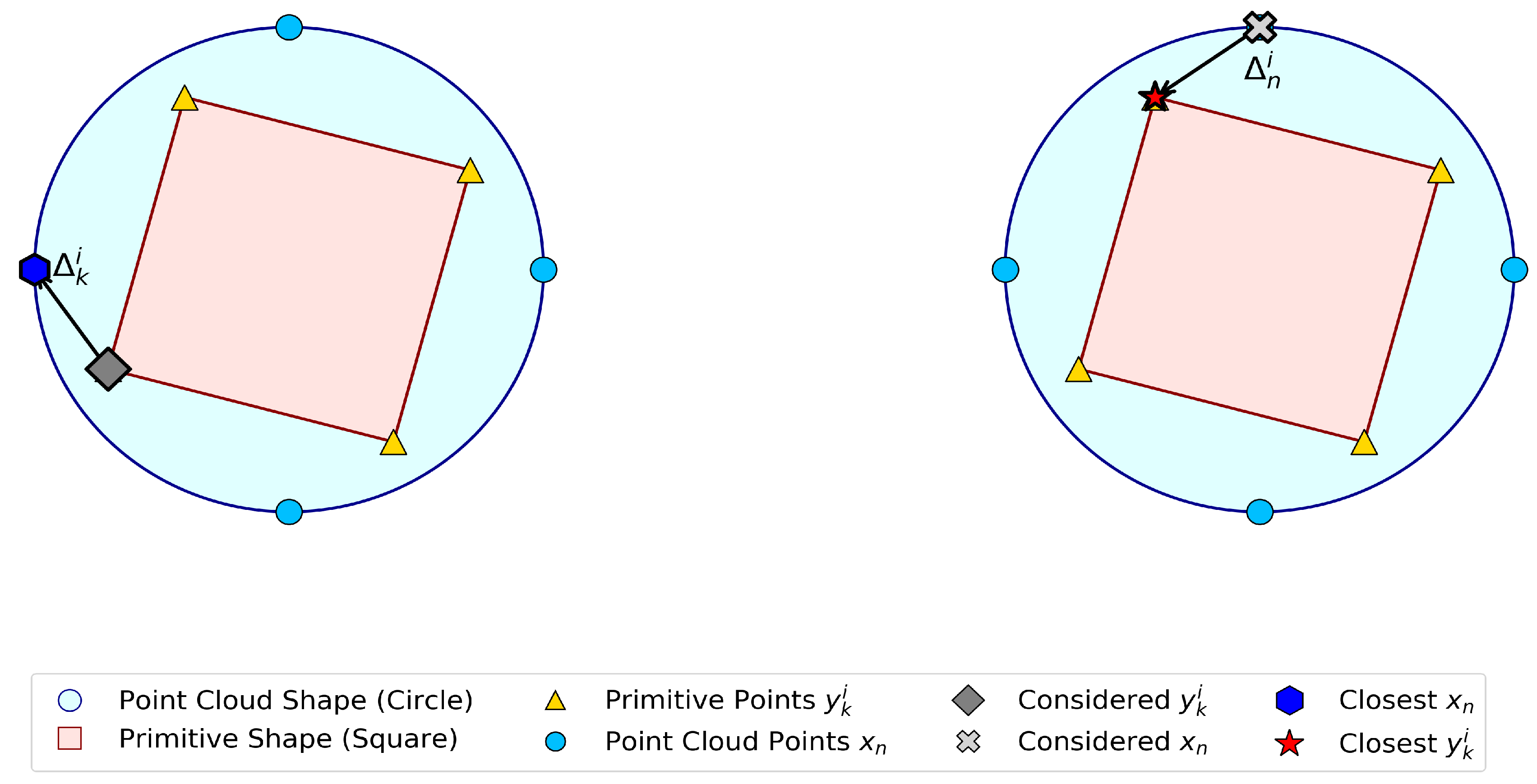
Figure 4.
Examples from the ShapeNet dataset illustrating the overlapping primitive problem in Eltaher and Breuß [6].
Figure 4.
Examples from the ShapeNet dataset illustrating the overlapping primitive problem in Eltaher and Breuß [6].
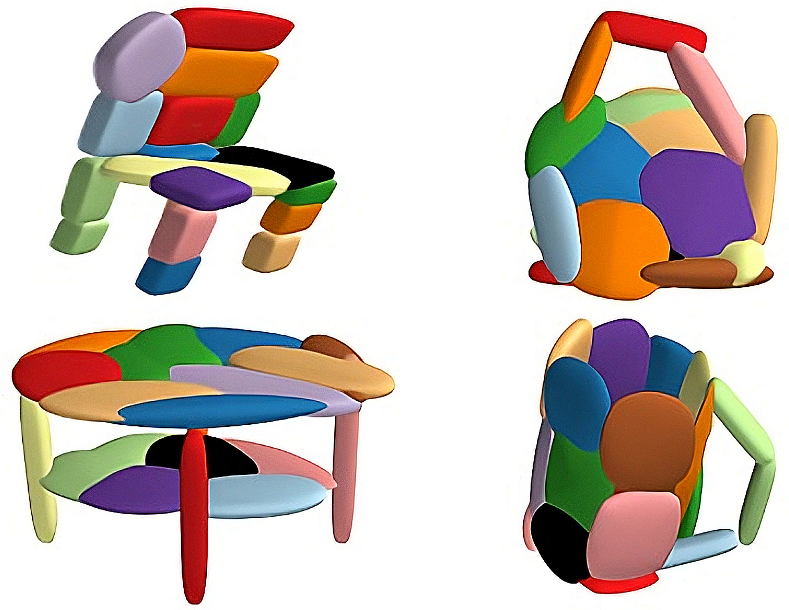
Figure 5.
Overview of the proposed deep learning framework. The PointNet encoder extracts a global feature vector from the input point cloud X, which is passed to four fully connected regressors that predict the parameters defining the size, shape, position, and orientation of superquadric primitives composing the reconstructed 3D object.
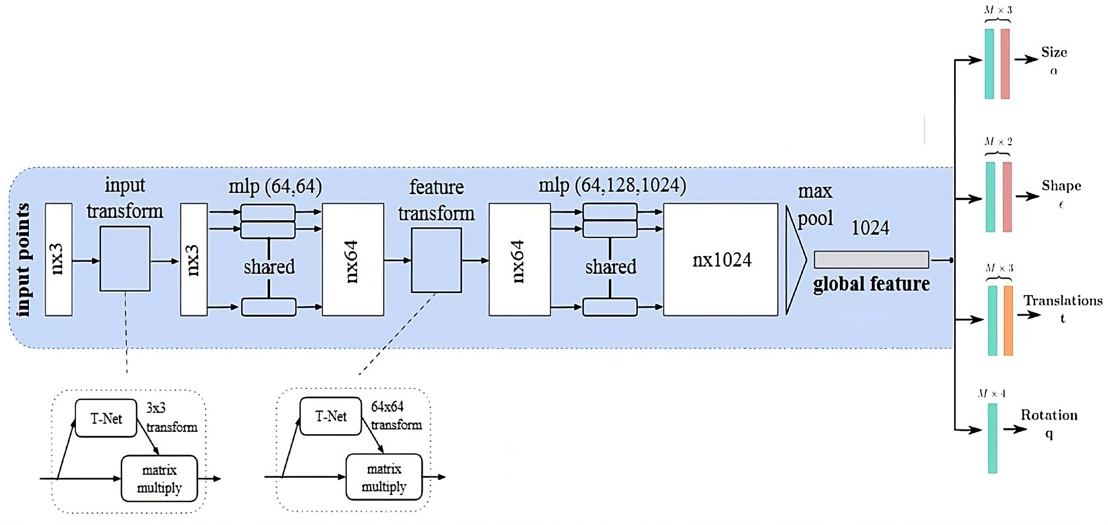
Figure 7.
Comparison of the baseline method [5] (first row) and Eltaher [6] (second row) on the ShapeNet dataset, showing qualitative results for old and new sampling strategies with different numbers of points (100 and 200).
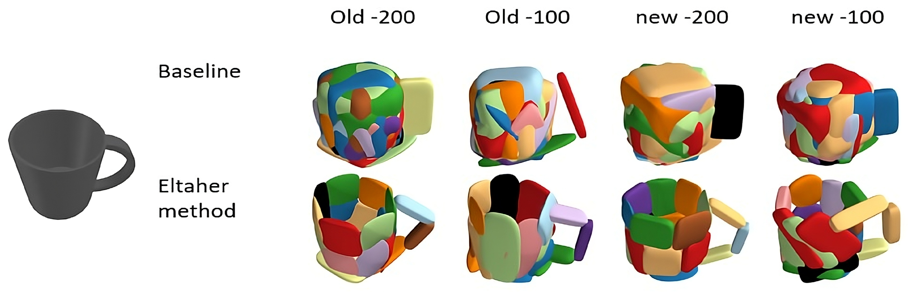
Figure 8.
Qualitative comparison on the ShapeNet dataset for the chair category, showing the baseline method [5] (first row), Eltaher [6] (second row), and our method (third row).
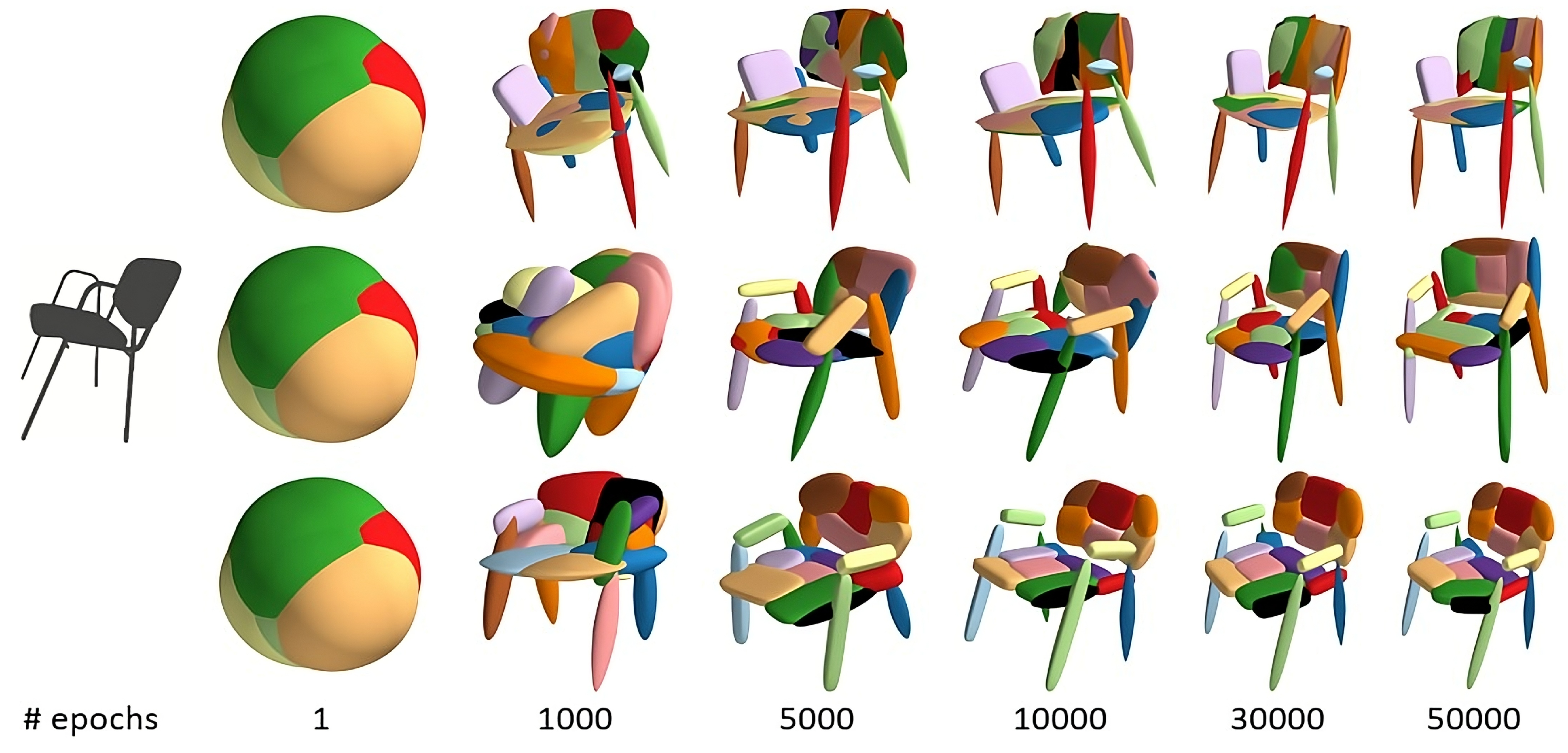
Figure 9.
Comparison of the overlapping Eltaher method [6] (first row) and Our discovery (second row) showing the difference in the overlapping in more details for the back and base chair sample.
Figure 9.
Comparison of the overlapping Eltaher method [6] (first row) and Our discovery (second row) showing the difference in the overlapping in more details for the back and base chair sample.
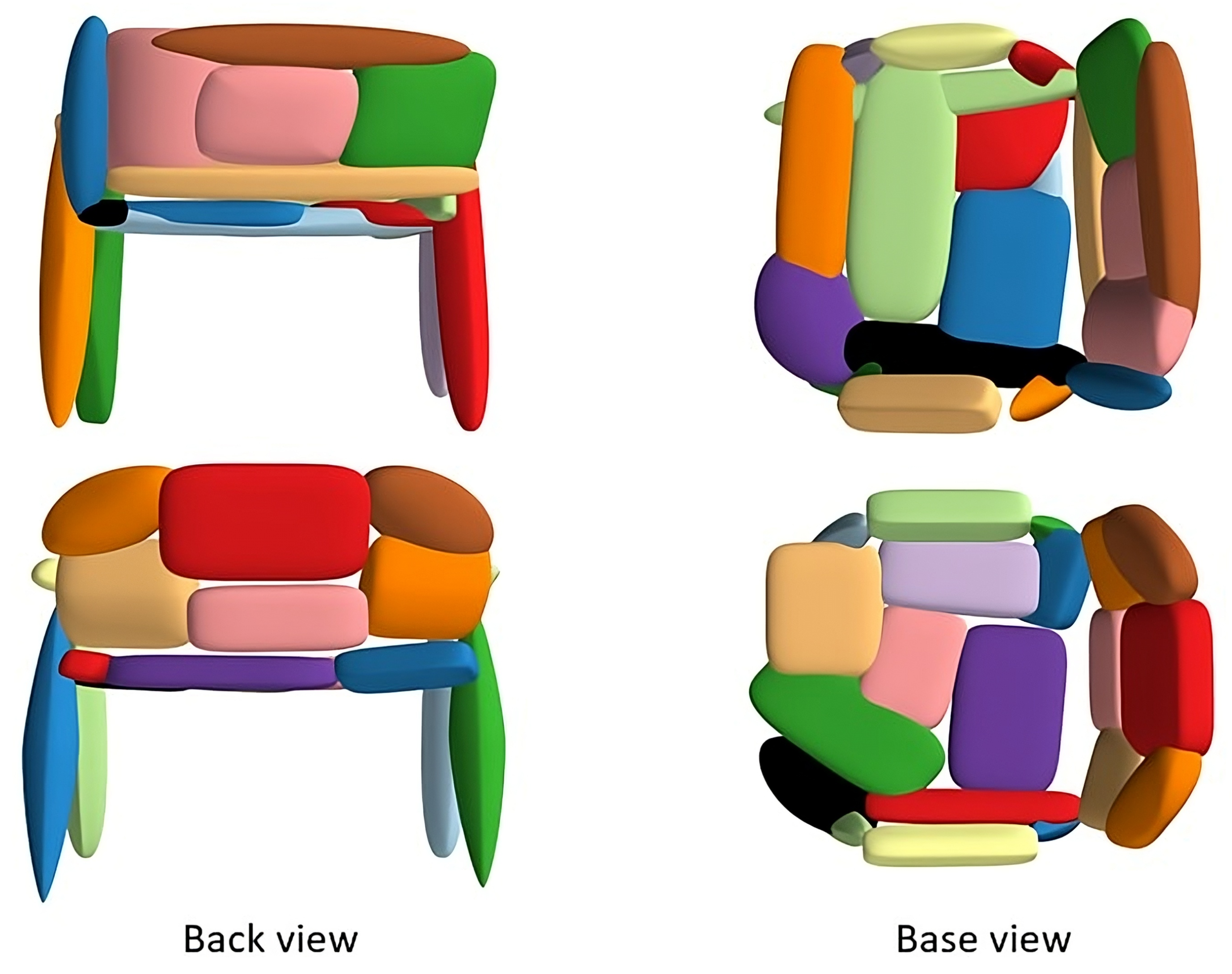
Figure 10.
Results on ShapeNet, (first-row) Input point cloud, (second-row) baseline result [5] ,(third-row) Eltaher results [6] ,(forth-row) our results .
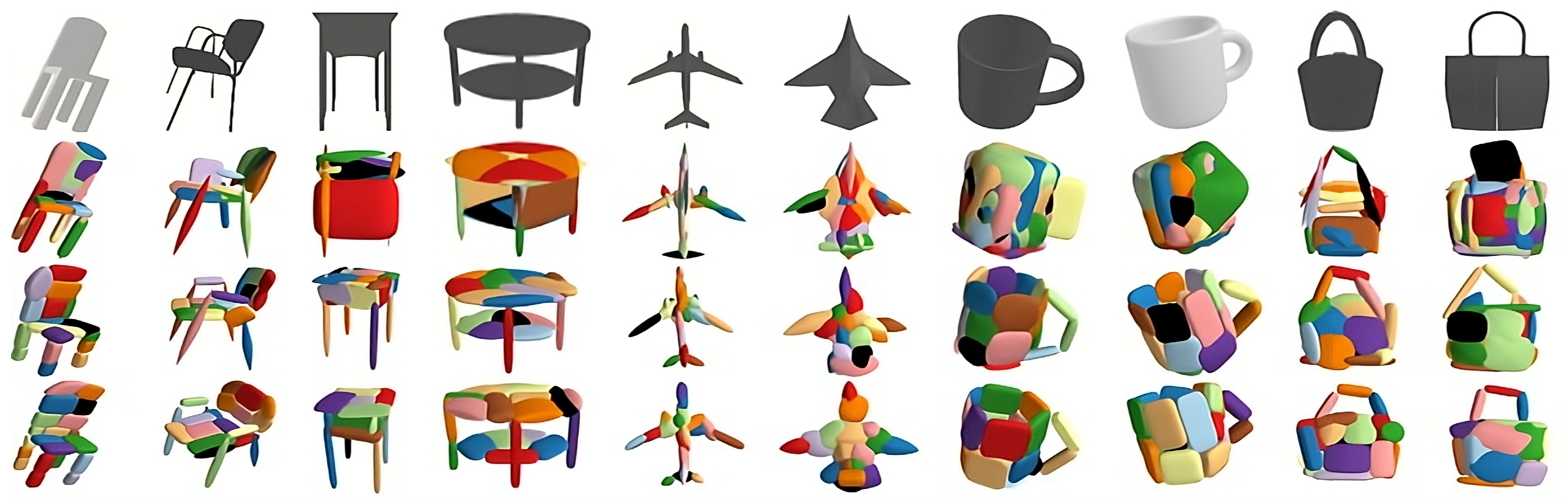
Table 1.
Geometric symbols, coordinate definitions, and indexing notation used throughout the paper.
Table 1.
Geometric symbols, coordinate definitions, and indexing notation used throughout the paper.
| Symbol | Definition |
|---|---|
| N | Total number of points in the input point cloud. |
| M | Total number of predicted primitives. |
| K | Number of surface points sampled on each primitive. |
| Set of input points associated with the i-th primitive. | |
| Coordinates of the n-th input point in the local coordinate system. | |
| P | Set of all sampled surface points from all predicted primitives. |
| X | Input point cloud, . |
| O | Set of points not covered by any predicted primitive (“outside” points). |
| i | Index over predicted primitives, . |
| k | Index over points sampled on each primitive, . |
| n | Index over points in the input point cloud, . |
Table 3.
Quantitative comparison of the baseline superquadric method [5] and the Eltaher method [6] under old and new sampling strategies on the ShapeNet dataset. For a fair comparison, the baseline method is re-evaluated using Kaiming initialization (which offers more stability than the original implementation). Results are computed over 10 runs on the Mug category. Note that structural accuracy and primitive accuracy are complementary metrics—improvement in one may lead to decline in the other.
| Method | Sampling | Statistic | Overlap (%) | Structural Accuracy | Primitive Accuracy | Corrected Precision |
|---|---|---|---|---|---|---|
| Baseline | Old | Max | 1.00 | 0.91 | 0.057 | 0.10 |
| Min | 0.99 | 0.88 | 0.000 | 0.00 | ||
| Avg | 0.99 | 0.90 | 0.036 | 0.10 | ||
| New | Max | 1.00 | 0.89 | 0.079 | 0.10 | |
| Min | 0.99 | 0.91 | 0.037 | 0.05 | ||
| Avg | 0.99 | 0.88 | 0.058 | 0.05 | ||
| Eltaher | Old | Max | 0.25 | 0.93 | 0.62 | 1.00 |
| Min | 0.15 | 0.86 | 0.58 | 0.95 | ||
| Avg | 0.20 | 0.90 | 0.59 | 0.95 | ||
| New | Max | 0.28 | 0.89 | 0.67 | 1.00 | |
| Min | 0.15 | 0.82 | 0.64 | 1.00 | ||
| Avg | 0.20 | 0.84 | 0.65 | 1.00 |
Table 4.
Quantitative comparison between the baseline superquadrics method [5] and Eltaher [6], using both old and new sampling strategies on the ShapeNet dataset. Two sampling densities (100 and 200 points) are evaluated for each strategy. For a fair comparison, the baseline method is implemented with Kaiming initialization (as used in Eltaher), which improves training stability over the original implementation. Results are averaged over 10 different runs on the mug category. Note that structural accuracy and primitive accuracy are complementary metrics – improving one may reduce the other.
| Method | Sampling | Points | Overlap (%) | Structural Accuracy | Primitive Accuracy | Corrected Precision |
|---|---|---|---|---|---|---|
| Baseline | Old | 200 | 0.99 | 0.90 | 0.036 | 0.10 |
| 100 | 0.99 | 0.90 | 0.037 | 0.05 | ||
| New | 200 | 0.99 | 0.90 | 0.077 | 0.10 | |
| 100 | 0.99 | 0.90 | 0.083 | 0.10 | ||
| Eltaher | Old | 200 | 0.20 | 0.90 | 0.60 | 1.00 |
| 100 | 0.28 | 0.91 | 0.61 | 1.00 | ||
| New | 200 | 0.20 | 0.84 | 0.70 | 1.00 | |
| 100 | 0.24 | 0.84 | 0.71 | 1.00 |
Table 5.
Effect of enabling overlapping on the baseline superquadrics method [5] and the Eltaher method [6]. For fair comparison, the baseline method uses Kaiming initialization, similar to our model. Results are averaged over 10 runs on the mug category from the ShapeNet dataset. Note: Structural Accuracy and Primitive Accuracy are complementary metrics – an improvement in one may lead to a decline in the other.
| Method | Overlapping Enabled | Overlap (%) | Structural Accuracy | Primitive Accuracy | Corrected Precision |
|---|---|---|---|---|---|
| Baseline | Without Overlapping | 0.99 | 0.88 | 0.036 | 0.10 |
| With Overlapping | 0.99 | 0.89 | 0.064 | 0.10 | |
| Eltaher | Without Overlapping | 0.24 | 0.93 | 0.60 | 1.00 |
| With Overlapping | 0.20 | 0.91 | 0.64 | 1.00 |
Table 6.
Comparison of superquadric-based reconstruction performance across categories (Chair, Airplane, Table) for the baseline [5], Eltaher [6], and our method. All methods use Kaiming initialization for consistency. Results are averaged over 20 input shapes per category from the ShapeNet dataset. Structural and primitive accuracies are complementary—an improvement in one may reduce the other.
| Category | Method | Overlap (%) | Structural Accuracy | Primitive Accuracy | Corrected Precision |
|---|---|---|---|---|---|
| Chair | Baseline | 0.89 | 0.81 | 0.55 | 0.75 |
| Eltaher | 0.30 | 0.94 | 0.52 | 0.85 | |
| Our Method | 0.22 | 0.92 | 0.61 | 1.00 | |
| Airplane | Baseline | 0.64 | 0.70 | 0.47 | 1.00 |
| Eltaher | 0.40 | 0.95 | 0.63 | 1.00 | |
| Our Method | 0.45 | 0.90 | 0.69 | 1.00 | |
| Table | Baseline | 0.97 | 0.78 | 0.44 | 0.60 |
| Eltaher | 0.33 | 0.96 | 0.43 | 0.70 | |
| Our Method | 0.24 | 0.90 | 0.69 | 1.00 |
Disclaimer/Publisher’s Note: The statements, opinions and data contained in all publications are solely those of the individual author(s) and contributor(s) and not of MDPI and/or the editor(s). MDPI and/or the editor(s) disclaim responsibility for any injury to people or property resulting from any ideas, methods, instructions or products referred to in the content. |
© 2025 by the authors. Licensee MDPI, Basel, Switzerland. This article is an open access article distributed under the terms and conditions of the Creative Commons Attribution (CC BY) license (http://creativecommons.org/licenses/by/4.0/).
Copyright: This open access article is published under a Creative Commons CC BY 4.0 license, which permit the free download, distribution, and reuse, provided that the author and preprint are cited in any reuse.