Submitted:
21 October 2025
Posted:
22 October 2025
You are already at the latest version
Abstract
Classical manifold learning methods such as Multidimensional Scaling (MDS), Isometric Mapping (Isomap), and Locally Linear Embedding (LLE) have played a pivotal role in nonlinear dimensionality reduction. While these approaches are well-established, a systematic empirical comparison under diverse data characteristics remains valuable for both research and practical applications. In this work, we present a comprehensive experimental evaluation of MDS, Isomap, and LLE, along with notable variants, across synthetic and real-world datasets of varying dimensionalities and structures. We assess their performance in terms of reconstruction error, runtime efficiency, and structural preservation, and analyze their behavior in different manifold settings. Our results reveal distinct strengths and limitations: LLE variants consistently excel on datasets with strong local geometric properties, while Isomap provides a favorable balance between runtime and structure preservation for high-dimensional image data. We also highlight the computational trade-offs of each method, providing practical guidelines for method selection in contemporary machine learning pipelines.
Keywords:
dimension reduction
; comparative study
1. Introduction
In high-dimensional data analysis, dimensionality reduction is a fundamental technique that enables effective data visualization, noise filtering, and computational efficiency. Feature Extraction Algorithms (FEAs) serve as a cornerstone in this process, transforming raw data into lower-dimensional representations while preserving essential structures. Among them, manifold-based FEAs have gained significant attention due to their ability to uncover nonlinear geometric structures inherent in complex datasets. These methods seek to preserve intrinsic relationships between data points, rather than relying on simple linear projections [1,2].
Within this paradigm, Multidimensional Scaling (MDS), Isometric Mapping (Isomap), and Locally Linear Embedding (LLE) represent three pivotal approaches that have shaped the evolution of manifold learning and nonlinear dimensionality reduction. MDS, initially developed for psychometrics and data visualization, provides a distance-preserving embedding. Isomap extends MDS by incorporating geodesic distances, making it effective for nonlinear structures. LLE, on the other hand, focuses on local geometric properties to reconstruct a globally consistent low-dimensional representation. These methods have been widely applied in various domains, including computer vision, bioinformatics, and robotics, demonstrating their enduring impact on data-driven research [3,4,5]. Despite their popularity, the choice among these methods is often guided by heuristic preferences rather than systematic performance evidence. Many prior studies focus either on theoretical derivations or on narrow experimental settings, leaving a gap in broad, quantitative comparisons across diverse datasets.
In this work, we conduct an empirical comparative study of MDS, Isomap, and LLE and their variants, evaluating them under controlled experiments across synthetic manifolds, low-dimensional tabular datasets, and high-dimensional image data. Despite the emergence of deep learning-based feature extraction techniques, MDS, Isomap, and LLE remain relevant due to their interpretability, efficiency, and adaptability in different scenarios. Understanding their theoretical foundations, practical applications, and comparative advantages is essential for researchers and practitioners seeking suitable dimensionality reduction techniques for their data. The key contributions are as follows:
- Algorithmic Workflows, Applications, and Complexity Analysis We summarize the core mathematical principles and computational processes of MDS, Isomap, and LLE. We highlight their respective application domains and discuss their computational complexity in large-scale settings.
- Conceptual and Empirical Comparisons We compare reconstruction error, runtime, and visualization quality, revealing the trade-offs between global and local structure preservation. We analyze their strengths, limitations, and suitability for various data structures, providing both theoretical insights and empirical validation.
- Adaptability in the Modern Era We examine the relevance of MDS, Isomap, and LLE in the context of large-scale data, deep learning advancements, and real-world applications. We discuss possible extensions and how these methods can be integrated into contemporary machine learning workflows.
2. Notation
The majority of manifold-based finite element analyses (FEAs) are nonlinear, unsupervised [6], and rely on neighborhood graphs [7]. These methods primarily concentrate on nonlinear mappings, assuming that the data, when projected into a lower-dimensional space, lies on a densely sampled manifold that needs to be unfolded [8,9]. Among these techniques, MDS, Isomap, and LLE are considered the classics. Table 1 presents the notations used in the paper.
3. Multi-Dimensional Scaling
Multidimensional Scaling (MDS) was introduced initially in [10] and stands as one of the pioneering techniques for dimensionality reduction [11]. It serves multiple purposes, including subspace learning, dimensionality reduction, and feature extraction. The core principle of MDS is to maintain the similarity [12] or dissimilarity/distances [13] between points in the low-dimensional space [2,14]. This approach enables MDS to capture the global structure of the data by fitting it locally [15]. MDS can be classified into three main types: classical MDS, metric MDS, and non-metric MDS [11,16], each of which will be discussed in this section. These categories yield distinct embedding results [17].
3.1. Classical Multidimensional Scaling
The goal of classical MDS is to preserve the similarity of the data points in the embedding space as it was in the input space [10]. One way to measure similarity is to calculate the inner product. Consequently, the difference between the similarities in the input and embedding spaces can be minimized by:
and we can extend it to a matrix form as:
and where denotes the Frobenius norm, and and are the Gram matrices of the original data X and the embedded data Y, respectively. We can then decompose the two Grame matrices using eigenvalue decomposition and get:
where and are obtained by squaring the singular values, after utilizing a Singular Value Decomposition (SVD) and by taking the right singular vectors of X and Y as V and Q, respectively. After mathematical proof and derivation[12], we can then obtain Y using:
Finally, we can truncate Y to , we can select the first p rows, which can result in a p-dimensional embedding of the n points.
3.2. Generalized Classical MDS (Kernel Classical MDS)
In the generalized setting, classical MDS is extended by allowing any valid kernel function to define the similarity matrix. Notably, Isomap can be seen as a special case of this approach, where geodesic distances are used instead of Euclidean distances [11].
As we get the Gram matrix in Section 3.1 we can give the Gram matrix as:
where D is the distance matrix with a squared Euclidean distance as its elements. Then by extending with a general kernel matrix, rather than the double-centered Gram matrix, we can have[11]:
where is the kernel matrix. for embedding X using classical MDS, the eigenvalue decomposition of the kernel matrix K is obtained in a similar way as Eq.(3):
Finally, we can get Y just as in Eq.(5), after a proper truncation and optimal selection, we can get top k dimention embedding of n points. We show the brief algorithm of generalized classical MDS in Algorithm .
| Algorithm 1:MDS |
|
Classical MDS with the Euclidean distance is equivalent to Principal Component Analysis (PCA). Moreover, the generalized classical MDS is equivalent to kernel PCA. This is a useful proposition we can use to further analyze the different extraction properties of two classical methods [18].
3.3. Metric Multidimensional Scaling
In classical Multidimensional Scaling (MDS), the focus is on maintaining the similarities between points in the embedding space. However, subsequent methods, such as Metric MDS, shifted the objective to preserving distances instead of similarities [19,20] within the embedding space [13]. Metric MDS aims to minimize the discrepancies in distances between points in both the input and embedding spaces [21]. The cost function used in Metric MDS is commonly known as the stress function [22,23]. This approach is termed "metric MDS" because it employs a distance metric for its optimization process.
The goal of metric MDS is to change the cost function to preserve the distances, rather than the similarities in the embedding space. In addition, metric MDS seeks to directly preserve pairwise distances in the embedded space, typically minimizing a stress function such as Kruskal’s stress. The objective function of metric MDS could be optimized by:
where the molecular part represents the normalization factors. Another well-known dimensionality reduction method Sammon Mapping [24], which is a special case of metric MDS.
3.4. Non-metric Multidimensional Scaling
Non-Metric Multidimensional Scaling (NMDS) is a variant of MDS that focuses on preserving the rank order of distances rather than their exact values [25,26]. Unlike metric MDS, which seeks to maintain precise pairwise distances, NMDS is more flexible and can handle non-Euclidean, nonlinear, or ordinal similarity measures. Instead of preserving absolute distances, it focuses on preserving the relative order of distances, making it robust to nonlinearly transformed similarity measures. This makes it particularly useful when the underlying data structure is unknown or when only qualitative comparisons (e.g., “A is more similar to B than to C”) are available. NMDS iteratively adjusts the low-dimensional representation to ensure that the ranking of distances in the embedded space closely matches the ranking in the original space, often optimizing a stress function such as Kruskal’s stress [27]. The objective can be generally written as:
Because of its robustness to distortions in absolute distances, NMDS is widely used in psychology, sociology, ecology, and market research, where perceptual or subjective similarity judgments are common.
4. Isometric Mapping
Isometric Mapping (Isomap) is a nonlinear dimensionality reduction technique designed to address the limitations of traditional methods like PCA and MDS, which struggle with preserving the intrinsic geometry of data lying on a nonlinear manifold [8,28]. Unlike these classical approaches that rely on Euclidean distances, Isomap reconstructs the manifold structure by maintaining geodesic distances between data points in the lower-dimensional space [2,14,29].
To achieve this, Isomap begins by constructing a neighborhood graph, where each data point is linked to its closest neighbors based on predefined criteria. It then estimates geodesic distances between all points by computing the shortest paths within this graph using algorithms such as Dijkstra’s or Floyd-Warshall [30]. The final step involves applying classical MDS to the computed geodesic distance matrix, ensuring that the low-dimensional representation retains the essential relationships present in the original high-dimensional space. Geodesic distance refers to the shortest path between two points along the surface or structure of a given space, rather than through the surrounding ambient space. In the context of manifold learning techniques like Isomap, geodesic distance is used to approximate the true intrinsic distance between data points that lie on a nonlinear manifold [31]. A simple comparison of Euclidian distance and geodeisic distance is shown in Figure 1.
The algorithm of Isomap is summarized in Algorithm 2.
| Algorithm 2:Isomap |
|
While Isomap has proven effective in capturing nonlinear structures, it is not without drawbacks. One major issue is its sensitivity to the quality of the neighborhood graph, which may introduce errors if incorrect connections are formed, leading to distortions in the final embedding.[32] Additionally, Isomap struggles with complex manifolds that contain discontinuities or non-convex regions, where geodesic distances may become unreliable. Despite these challenges, Isomap remains widely used in various scientific and engineering applications, including face recognition, motion analysis, and medical imaging, due to its ability to reveal meaningful low-dimensional representations of high-dimensional data [33].
5. Locally Linear Embedding
Locally Linear Embedding (LLE) is a widely recognized nonlinear spectral dimensionality reduction technique, primarily designed for manifold learning and feature extraction [34,35,36]. Unlike traditional linear techniques such as PCA or MDS, LLE preserves the local geometric structure of high-dimensional data while mapping it to a lower-dimensional space [37]. This is achieved by approximating each data point as a weighted linear combination of its nearest neighbors in the original space and ensuring that these relationships remain consistent in the embedded space [2,38].
The algorithm follows a three-step process: (1) identifying the K nearest neighbors for each data point, (2) computing the optimal reconstruction weights that best express each point as a linear combination of its neighbors, and (3) finding a low-dimensional embedding that preserves these relationships [15,39]. By focusing on local neighborhood structures rather than global variance, LLE effectively captures the intrinsic geometry of nonlinear manifolds, making it a powerful tool for dimensionality reduction [40].
Given a dataset of N points in a D-dimensional space, LLE first constructs a neighborhood graph by identifying the K nearest neighbors of each point based on Euclidean distance. Then, it computes the reconstruction weights by approximating each data point as a weighted linear combination of its neighbors, minimizing the reconstruction error:
subject to the constraint:
These weights are obtained by solving a constrained least-squares problem. Finally, LLE determines the low-dimensional embeddings by minimizing:
This step corresponds to finding the eigenvectors associated with the smallest nonzero eigenvalues of the matrix:
where W is the weight matrix containing . The final low-dimensional representation is given by the eigenvectors corresponding to the smallest d nonzero eigenvalues. LLE is widely used in manifold learning as it effectively preserves local geometric structures without assuming global linearity.
The algorithm of LLE is summarized in Algorithm 3.
| Algorithm 3:LLE |
|
LLE has been widely applied across various domains, including image processing, bioinformatics, and network analysis [41,42]. In particular, it has shown effectiveness in medical diagnosis applications, where high-dimensional patient data is embedded into a meaningful lower-dimensional representation for classification and visualization [43]. Furthermore, LLE has been successfully used for analyzing astronomical spectra, demonstrating its versatility in handling complex scientific data [44]. However, despite its advantages, LLE has some limitations, including sensitivity to noise and difficulties in handling non-convex manifolds [35].
The advantage of LLE is its proficiency in managing nonlinear data and sparse matrices. Consequently, it may demand less computational time and space compared to other feature extraction methods. Overall, LLE offers a unique approach to nonlinear dimensionality reduction by leveraging local linear reconstructions to uncover meaningful global embeddings. Its ability to maintain local relationships while reducing dimensionality makes it a valuable technique in manifold learning and data-driven applications [36,37].
6. Contemporary Relevance and Applications
In contemporary applications, Multi-Dimensional Scaling (MDS), Isomap, and Locally Linear Embedding (LLE) are vital for analyzing high-dimensional data. While MDS excels at preserving pairwise dissimilarities in linear spaces, it struggles with nonlinear relationships. Isomap overcomes this by incorporating geodesic distances, making it ideal for data on nonlinear manifolds [34]. LLE further enhances this by maintaining local geometric structures, allowing it to model complex manifolds effectively [35]. These techniques are widely used in fields such as image processing, medical diagnostics, and bioinformatics, offering powerful tools for dimensionality reduction and data visualization. In addition, some of these methods are still active in modern machine learning systems, and has been widely used in multiple fields like quantum physics and multi-class data augmentation of wind [45,46]. A summary of development and applications of MDS, Isomap, and LLE is shown in Table 2.
7. Experiments
7.1. Datasets
We use four different datasets, encompassing synthetic and real-world data, numerical data and images, as well as both regression and classification tasks, to provide a comprehensive comparison of MDS, Isomap, and LLE. The datasets are summarized in Table 3.
7.2. Methods
In the context of MDS, we examine both metric MDS and non-metric MDS, along with Isomap, which can also be regarded as a special case of kernel classical MDS. In addition to standard LLE, we consider two variants: HLLE [76] and MLLE [76]. Hessian LLE (HLLE) improves the robustness of LLE by using Hessian-based constraints to better preserve local geometric structures. Modified LLE (MLLE) tackles the problem of short-circuiting in manifolds by adjusting the reconstruction weights, ensuring more accurate modeling of complex data structures. The visualization of the six methods are shown in Section 7.3.
Aside from the methods based on MDS, Isomap and LLE, we also utilize several classical methods for visualization experiments, including PCA [77], LTSA [78], Kernel PCA [77], Laplacian Eigenmaps [79], and t-SNE [80]. The overall visualization results are shown in Appendix (Appendix A).

Table 4.
Runtime and Error Comparisons of Dimensionality Reduction Methods Across Datasets
| Method | SwissRoll | Iris | AutoMPG | MNIST | ||||
|---|---|---|---|---|---|---|---|---|
| Runtime (s) | Error | Runtime (s) | Error | Runtime (s) | Error | Runtime (s) | Error | |
| Metric MDS | 6.28 | 5.9e+06 | 0.16 | 1.6e+02 | 1.55 | 2.3e+06 | 0.59 | 4.1e+10 |
| Non-metric MDS | 2.12 | 2.3e+04 | 0.04 | 5.1e+02 | 0.30 | 3.5e+03 | 0.14 | 2.0e+03 |
| Isomap | 0.35 | 1.0e+01 | 0.02 | 1.2e-01 | 0.13 | 1.4e+03 | 0.04 | 1.0e+06 |
| Standard LLE | 0.09 | 2.2e-07 | 0.01 | 2.9e-05 | 0.08 | 1.1e-03 | 1.01 | 2.0e-03 |
| Hessian LLE | 0.18 | 4.8e-06 | 0.03 | 1.1e-01 | 0.21 | 1.4e-01 | 6.49 | 2.4e+01 |
| Modified LLE | 0.14 | 2.2e-06 | 0.03 | 2.5e-01 | 0.20 | 6.2e-01 | 6.97 | 1.7e+02 |
7.3. Visualization Results
Figure 2.
SwissRoll visualization results.
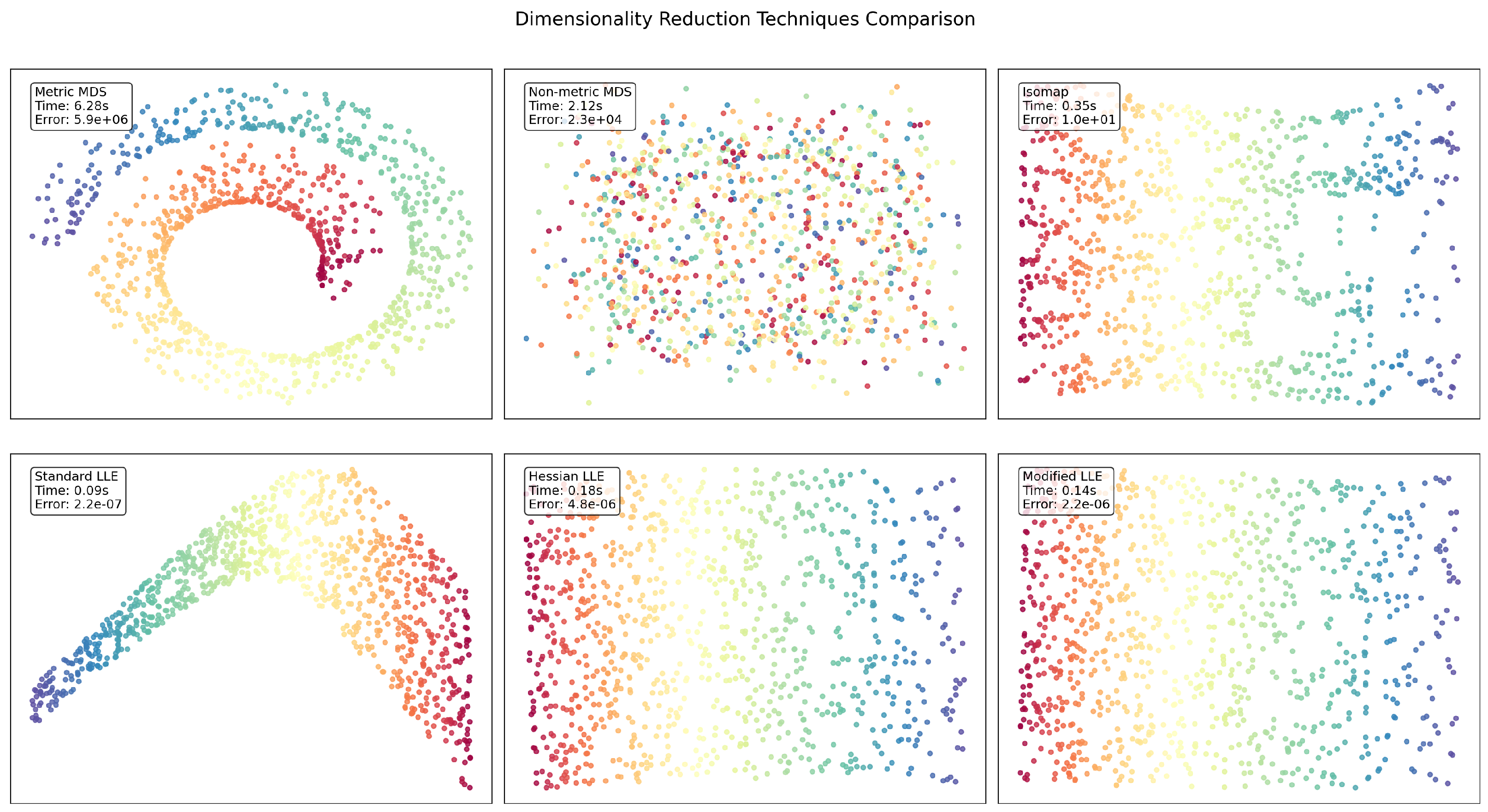
Figure 3.
Iris visualization results.
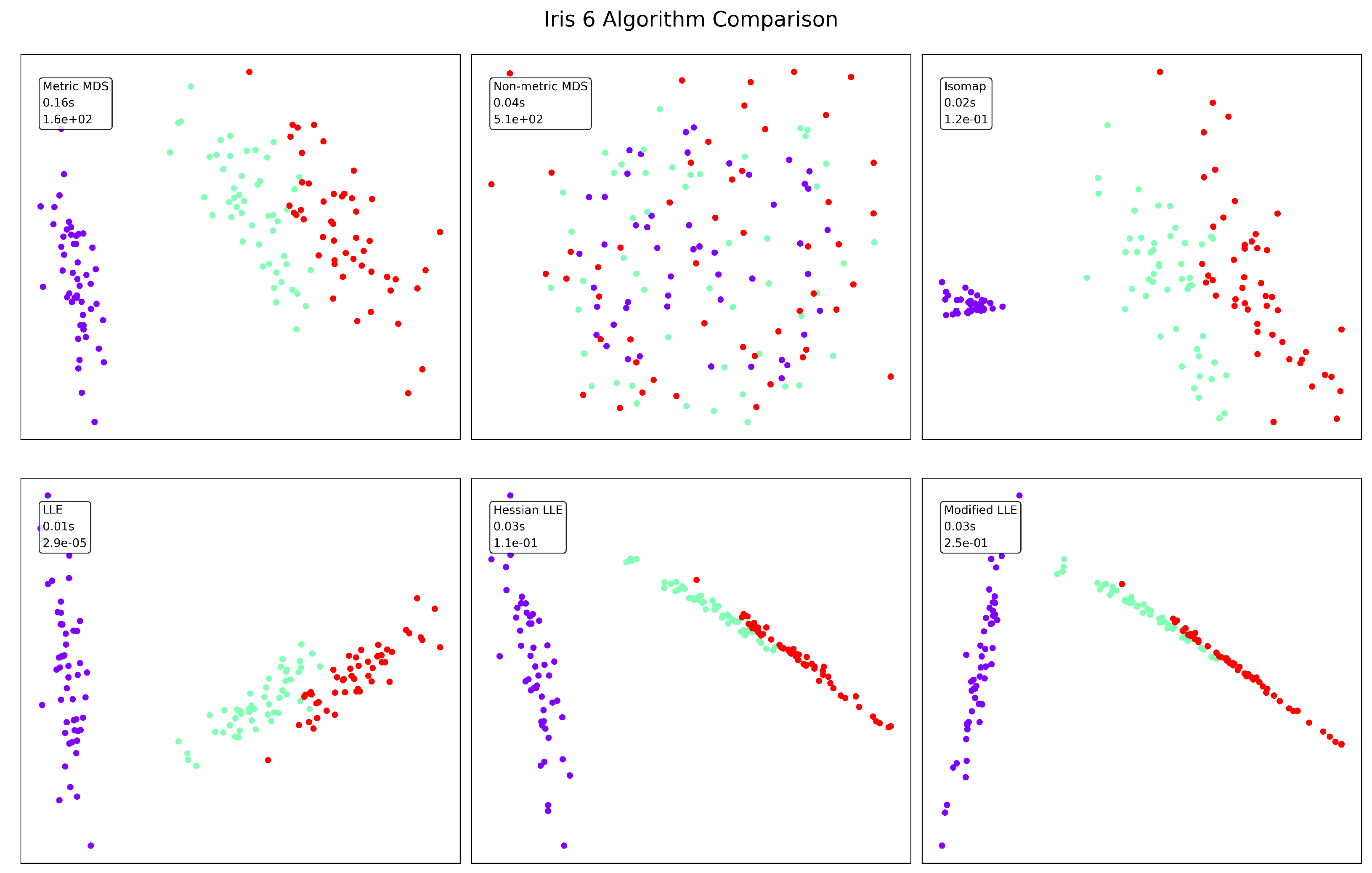
Figure 4.
AutoMPG visualization results.
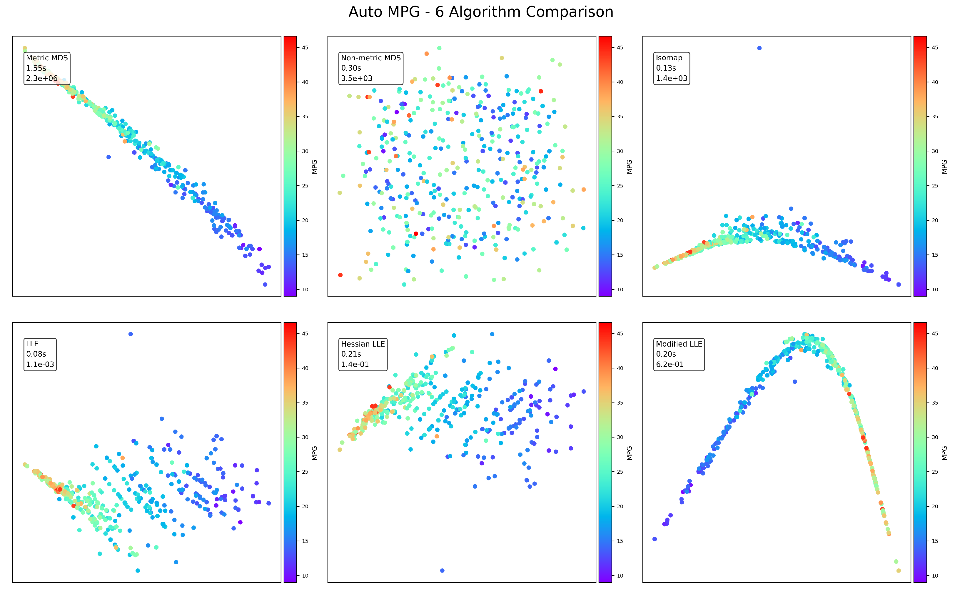
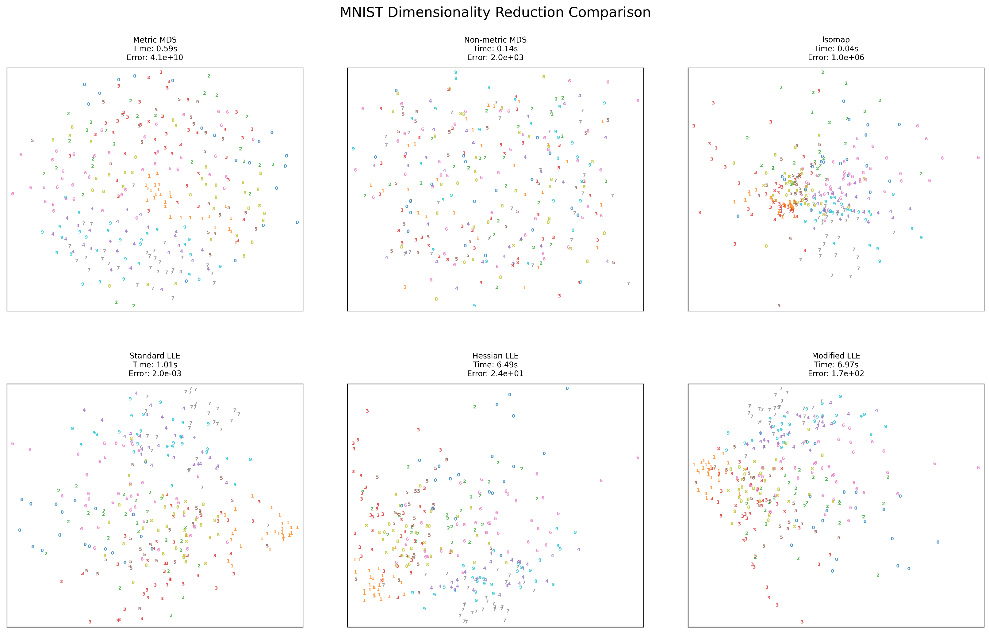
Figure 5.
MNIST visualization results.
The SwissRoll dataset reveals striking differences between the techniques. In terms of error performance, Standard LLE dramatically outperforms other methods with an error () that is approximately 10 orders of magnitude lower than Metric MDS (). Standard LLE is also the fastest method (0.09s), while Metric MDS is significantly slower (6.28s). Regarding visual structure, LLE variants preserve the intrinsic manifold structure, displaying a coherent circular or curved pattern, whereas Non-metric MDS fails to capture meaningful structure. The superior performance of LLE methods suggests this dataset has strong local geometric properties that are well-preserved by neighborhood-based approaches.
The well-known Iris dataset presents different characteristics compared to the synthetic manifold. Standard LLE again achieves the lowest error (), but Isomap (0.02s) and Non-metric MDS (0.04s) offer competitive runtime performance. In terms of clustering quality, LLE variants and Isomap effectively separate the three classes (likely corresponding to the three Iris species), while Non-metric MDS produces poor separation. Hessian and Modified LLE produce more linear arrangements of the data points, potentially revealing the known characteristic that one Iris species is linearly separable from the other two. The moderate dimensionality of the Iris dataset (4 features) likely contributes to the overall good performance across most methods.
The AutoMPG dataset reveals interesting patterns related to fuel efficiency. Standard LLE maintains its error advantage (), but the gap narrows compared to other datasets. Modified LLE and Metric MDS produce the most visually interpretable projections, clearly showing the gradient from high to low MPG values. The curved structures revealed by several methods (particularly Modified LLE’s U-shape) suggest that vehicle efficiency follows non-linear relationships in the feature space. Interestingly, Metric MDS produces a visually coherent projection despite its high error (), highlighting that mathematical error doesn’t always correlate with visual interpretability.
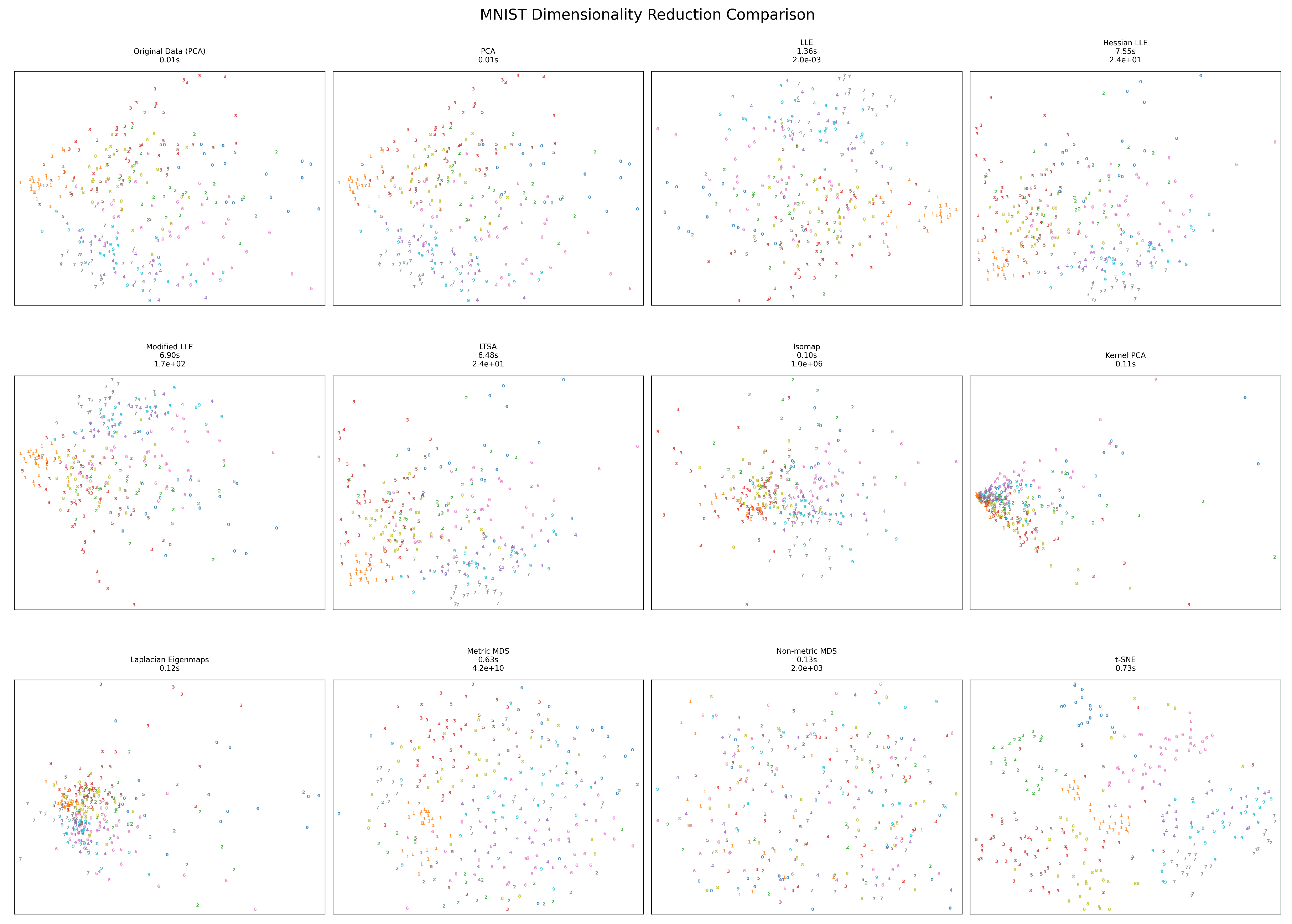
The high-dimensional MNIST handwritten digit dataset (784 dimensions) presents unique challenges for dimensionality reduction. LLE variants become significantly slower (6.49s and 6.97s for Hessian and Modified LLE, respectively) compared to other methods and other datasets. Metric MDS produces an extremely high error (), while Standard LLE maintains a remarkably low error (). Standard LLE produces the most effective separation of digit classes, though several methods show similar digits (e.g., 1 and 7) clustering together. Isomap offers the best balance of speed (0.04s) and reasonable structure preservation for this high-dimensional dataset.
7.4. Temporal Complexity Analysis
In terms of computational complexity, MDS is generally the most computationally expensive among the three methods, as it requires calculating a distance matrix and performing eigenvalue decomposition, which can become slow for large datasets. Isomap involves additional steps such as constructing a neighborhood graph and calculating the shortest paths between points, making it more complex than MDS, especially as the dataset grows. LLE, while similar to Isomap in that it requires a nearest-neighbor search and eigen-decomposition, tends to be more efficient in handling sparse data structures. However, it can still be computationally expensive due to the need to solve for reconstruction weights. Overall, Isomap and LLE are more complex than MDS, with Isomap requiring more memory and processing due to the shortest-path calculations, while LLE can be more efficient for sparse data but still demands significant computation for larger datasets. We show the complexity comparison of MDS, Isomap, and LLE in Table 5.
Overall, we make a general comparison of MDS, Isomap, and LLE in Table 5.
Table 6.
General Comparison of MDS, Isomap, and LLE.
| Goal | Supervision | Linearity | Data Charac. | Iteration | Topology | |
|---|---|---|---|---|---|---|
| MDS | Preserve Euclidean pairwise distances | Unsuper. | Nonlinear | Perform better with relational data | Yes | Manifold |
| Isomap | Preserve geodesic pairwise distances | Unsuper./Super. | Nonlinear | Handle sparse and noisy data | No | Manifold |
| LLE | Preserve local properties | Unsuper. | Nonlinear | Handle sparse and nonlinear data | Yes | Manifold |
8. Adaptibility in the Modern Era
With the advancement of deep learning technologies, an increasing number of traditional methods are being replaced by deep learning in the modern era. In this rapidly evolving technological landscape, it is worth exploring how traditional methods like MDS, Isomap, and LLE can be adapted, refined, or integrated into contemporary approaches.
Selecting an appropriate dimensionality reduction technique for high-dimensional data, such as images, requires careful consideration of multiple factors including data characteristics, computational resources, preservation requirements, and the intended downstream tasks. Classical methods like MDS, Isomap, and LLE, alongside modern deep learning approaches [81], each present distinct advantages and limitations.
The intrinsic dimensionality and structure of the data should guide initial method selection. MDS techniques emphasize distance preservation and work well when global distances are meaningful, with metric MDS preserving Euclidean distances and non-metric MDS focusing on ordinal relationships. For image data, however, Euclidean distances often fail to capture perceptual similarity, limiting the effectiveness of standard MDS. When images are believed to lie on or near a manifold, manifold learning approaches become more appropriate. Isomap extends MDS by approximating geodesic distances along the manifold through neighborhood graphs, making it suitable for data with curved but smooth underlying structure. LLE and its variants (Hessian, Modified) focus on preserving local relationships by reconstructing each point from its neighbors, often yielding better results for image data where local pixel relationships are more meaningful than global distances.
For high-dimensional image datasets, computational considerations become paramount. Standard implementations of MDS and Isomap scale poorly. Several strategies can mitigate these limitations: landmark points [82,83]; incremental variants compute embeddings for new points without recalculating the entire solution [84]; and spectral approximation techniques can improve efficiency [85,86]. For extremely large image datasets (e.g., millions of images), sampling representative subsets before applying classical methods often becomes necessary.
Deep learning methods, such as Variational Autoencoders (VAEs) [87] and Generative adversarial networks (GANs) [88], offer compelling alternatives for high-dimensional image data. VAEs combine the reconstruction capability of autoencoders with probabilistic modeling, creating smooth, continuous latent spaces that facilitate generation and interpolation. Their non-linear transformations can capture complex relationships in image data that linear methods miss. Similarly, GANs incorporate discriminator networks to match latent distributions to prior distributions, often yielding more structured latent spaces. These deep learning approaches scale well with data dimensionality, though they typically require substantial data volumes and training time.
For practical implementation with image data, several preprocessing steps can significantly improve results. Downsampling high-resolution images reduces dimensionality while preserving essential structural information. Feature extraction using pre-trained convolutional neural networks (e.g., extracting activations from intermediate layers of VGG networks[89] or ResNet [90]) can provide semantically meaningful representations before applying classical dimensionality reduction. Color space transformations (RGB to Lab or HSV) can also yield representations where distances better align with perceptual similarity.
Hybrid approaches often yield superior results for image data. For instance, applying t-SNE or UMAP to features extracted from pre-trained neural networks combines the perceptual understanding of deep networks with the visualization strength of manifold learning. Similarly, using classical methods to initialize latent spaces for deep learning models can accelerate convergence and improve results. Evaluation criteria should match the intended application. For visualization, qualitative assessment of cluster separation and structure preservation may suffice. For downstream tasks like classification, performance metrics on the reduced representation provide objective evaluation. Reconstruction error offers a direct measure of information preservation, while neighborhood preservation metrics (e.g., trustworthiness and continuity) evaluate how well local relationships are maintained.
No single dimensionality reduction technique universally outperforms others across all high-dimensional data scenarios. For image data specifically, deep learning methods generally excel at capturing complex patterns and generating new samples, while manifold learning approaches like Isomap and LLE often provide more interpretable visualizations of data structure. Practical applications frequently benefit from combining approaches—using deep networks for feature extraction followed by classical methods for final dimensionality reduction and visualization. This integrated strategy leverages the complementary strengths of different approaches while mitigating their individual limitations.
9. Conclusions
In this thesis, we compared three dimensionality reduction techniques: Multidimensional Scaling (MDS), Isometric Mapping (Isomap), and Locally Linear Embedding (LLE). Each method has its own strengths and weaknesses, making them suitable for different types of datasets.
- MDS works well for linear datasets, preserving global pairwise distances, but struggles with non-linear structures and can be computationally expensive.
- Isomap extends MDS by incorporating geodesic distances, making it suitable for non-linear manifolds, though it can be computationally intensive and sensitive to noisy data.
- LLE excels at preserving local structures in non-linear datasets, but requires careful tuning and is sensitive to noise in high-dimensional spaces.
Our findings suggest that the choice of method should be guided by the dataset’s intrinsic structure and the specific objectives of the analysis. MDS is preferable when global distance preservation is crucial, Isomap is effective for nonlinear manifolds, and LLE excels at capturing local nonlinear relationships. In most cases, nonlinear FEAs performed better than linear FEAs. In conclusion, the choice of method depends on the dataset’s structure and the task’s objectives. Each method possesses distinct advantages, and future research may explore hybrid approaches that harness their strengths or integrate them with deep learning techniques to enhance scalability and robustness.
Appendix A
The visualization results of all methods for the four datasets are shown in Figure A1–Figure A4. The first subfigure shows the visualization of the dataset (only the first two dimensions are displayed for data with more than three dimensions). Code for reproducing all the experimental results can be accessed through https://github.com/SoftPointer/dimensionality_reduction.
Figure A1.
SwissRoll visualization results (overall).
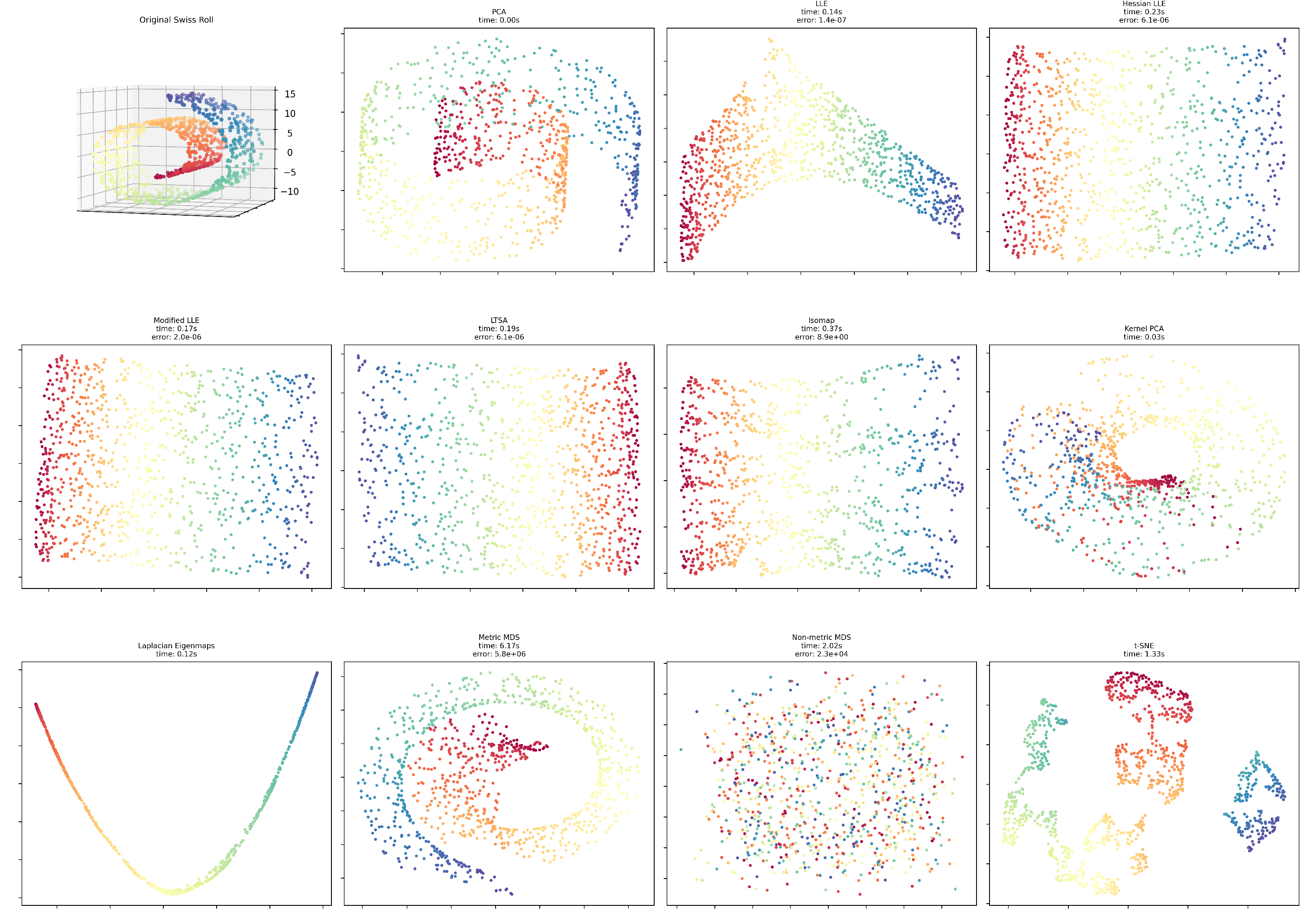
Figure A2.
Iris visualization results (overall).
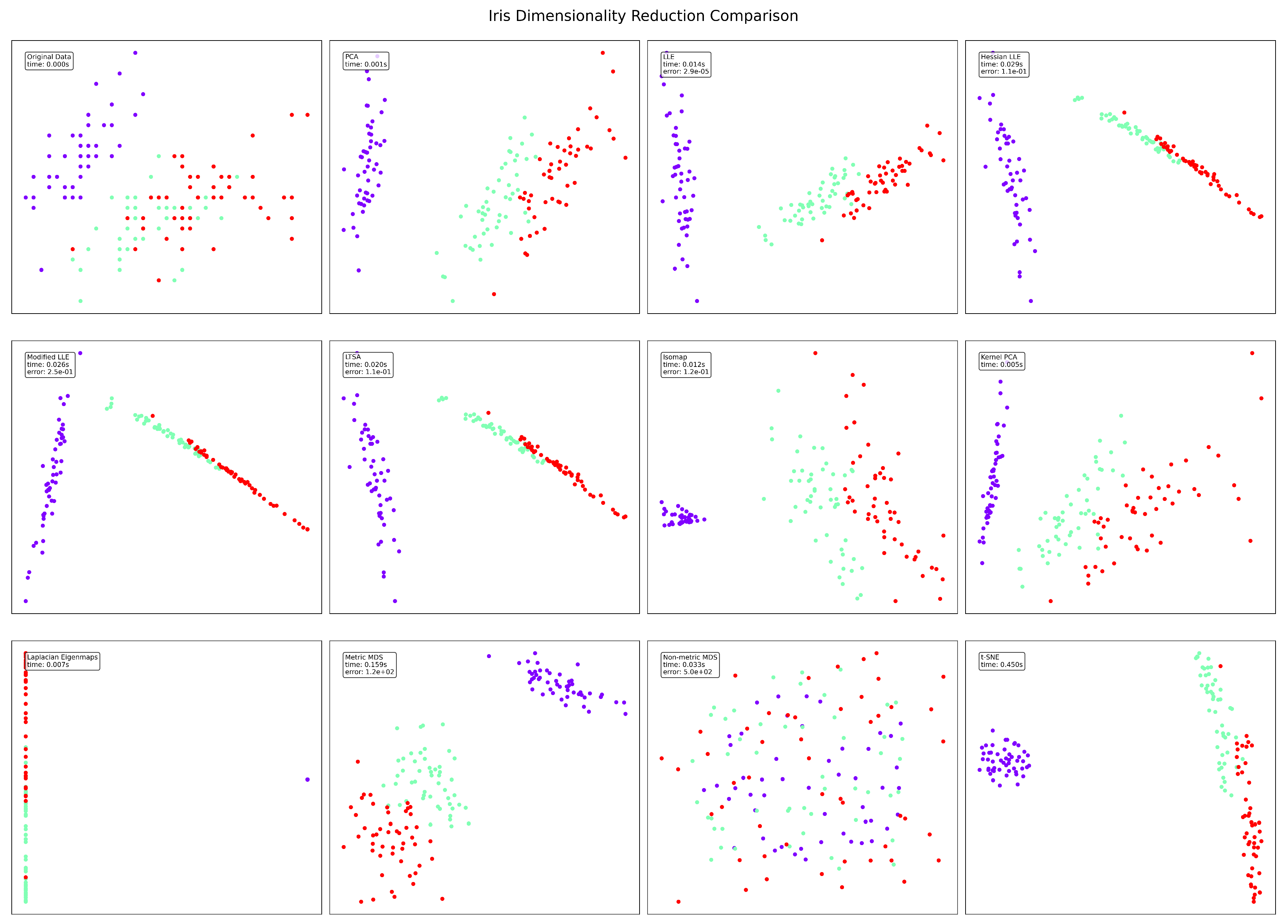
Figure A3.
AutoMPG visualization results (overall).
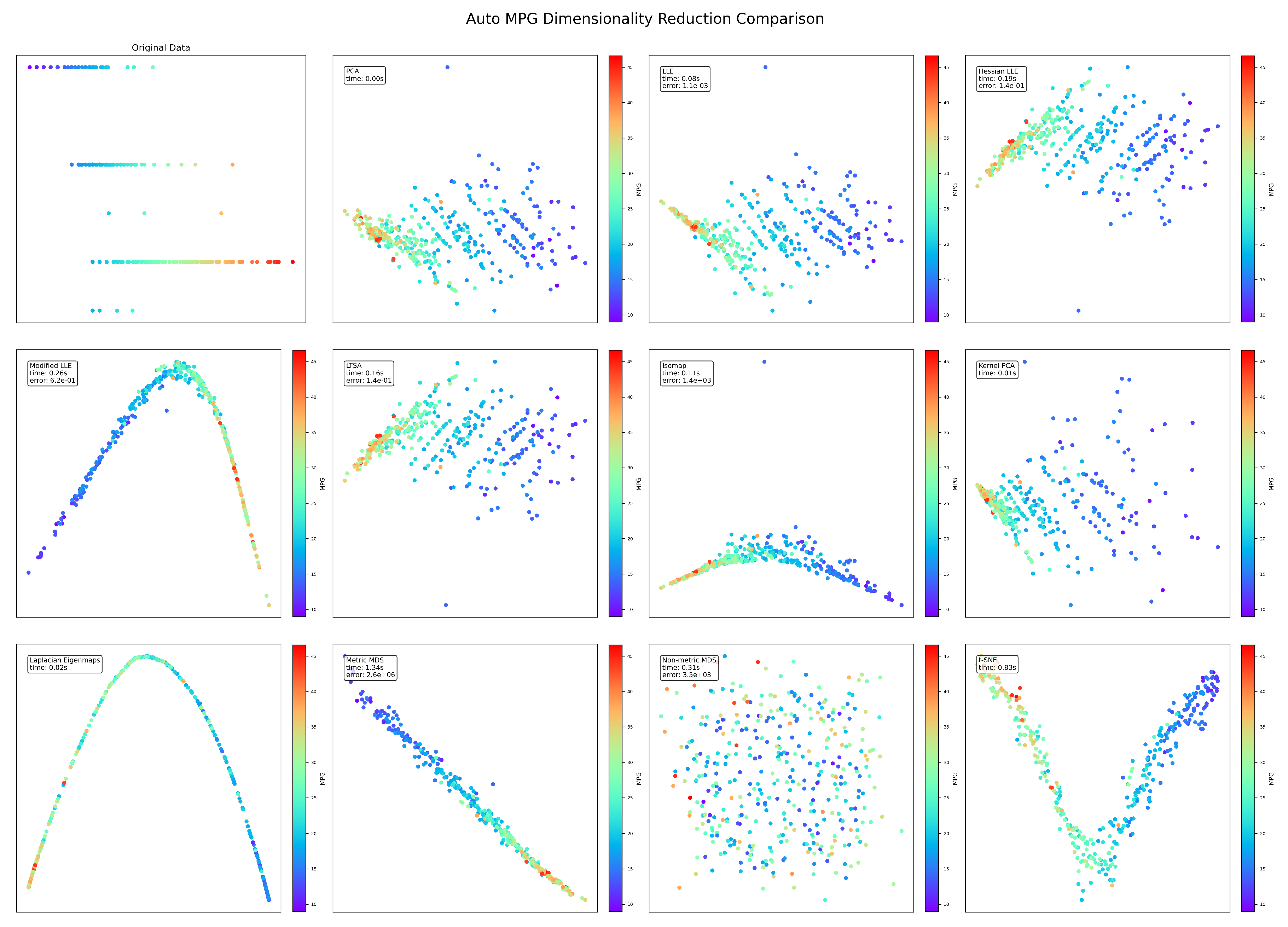
Figure A4.
MNIST visualization results (overall).
References
- M. H. Law and A. K. Jain, “Incremental nonlinear dimensionality reduction by manifold learning,” IEEE transactions on pattern analysis and machine intelligence, vol. 28, no. 3, pp. 377–391, 2006.
- B. Ghojogh, M. Crowley, F. Karray, and A. Ghodsi, Elements of dimensionality reduction and manifold learning. Springer, 2023.
- J. B. Kruskal and M. Wish, Multidimensional scaling. Sage, 1978, no. 11.
- Y. Wang, Z. Zhang, and Y. Lin, “Multi-cluster feature selection based on isometric mapping,” IEEE/CAA Journal of Automatica Sinica, vol. 9, no. 3, pp. 570–572, 2021.
- S. T. Roweis and L. K. Saul, “Nonlinear dimensionality reduction by locally linear embedding,” science, vol. 290, no. 5500, pp. 2323–2326, 2000.
- F. Pedregosa, G. Varoquaux, A. Gramfort, V. Michel, B. Thirion, O. Grisel, M. Blondel, P. Prettenhofer, R. Weiss, V. Dubourg et al., “Scikit-learn: Machine learning in python,” the Journal of machine Learning research, vol. 12, pp. 2825–2830, 2011.
- M. Sedlmair, M. Brehmer, S. Ingram, and T. Munzner, “Dimensionality reduction in the wild: gaps and guidance. department of computer science, university of british columbia, vancouver, bc,” Canada, Technical report TR-2012-03, Tech. Rep., 2012.
- L. Van Der Maaten, E. O. Postma, H. J. Van Den Herik et al., “Dimensionality reduction: A comparative review,” Journal of machine learning research, vol. 10, no. 66-71, p. 13, 2009.
- F. Anowar, S. Sadaoui, and B. Selim, “Conceptual and empirical comparison of dimensionality reduction algorithms (pca, kpca, lda, mds, svd, lle, isomap, le, ica, t-sne),” Computer Science Review, vol. 40, p. 100378, 2021.
- W. S. Torgerson, “Multidimensional scaling: I. theory and method,” Psychometrika, vol. 17, no. 4, pp. 401–419, 1952.
- T. F. Cox and M. A. Cox, Multidimensional scaling. CRC press, 2000.
- W. S. Torgerson, “Multidimensional scaling of similarity,” Psychometrika, vol. 30, no. 4, pp. 379–393, 1965.
- R. Beals, D. H. Krantz, and A. Tversky, “Foundations of multidimensional scaling.” Psychological review, vol. 75, no. 2, p. 127, 1968.
- Ghojogh, A. Ghodsi, F. Karray, and M. Crowley, “Multidimensional scaling, sammon mapping, and isomap: Tutorial and survey,” arXiv preprint arXiv:2009.08136, 2020.
- L. K. Saul and S. T. Roweis, “Think globally, fit locally: unsupervised learning of low dimensional manifolds,” Journal of machine learning research, vol. 4, no. Jun, pp. 119–155, 2003.
- I. Borg and P. J. Groenen, Modern multidimensional scaling: Theory and applications. Springer Science & Business Media, 2007.
- S. Jung, “Lecture 8: Multidimensional scaling-advanced applied multivariate analysis,” Lecture notes, Department of Statistics, University of Pittsburgh, 2013.
- T. Hofmann, B. Schölkopf, and A. J. Smola, “Kernel methods in machine learning,” 2008.
- K. Bunte, M. Biehl, and B. Hammer, “A general framework for dimensionality-reducing data visualization mapping,” Neural Computation, vol. 24, no. 3, pp. 771–804, 2012.
- J. A. Lee and M. Verleysen, Nonlinear dimensionality reduction. Springer Science & Business Media, 2007.
- A. Ghodsi, “Dimensionality reduction a short tutorial,” Department of Statistics and Actuarial Science, Univ. of Waterloo, Ontario, Canada, vol. 37, no. 38, p. 2006, 2006.
- J. De Leeuw, “Multidimensional scaling,” 2011.
- K. V. Mardia, “Some properties of clasical multi-dimesional scaling,” Communications in Statistics-Theory and Methods, vol. 7, no. 13, pp. 1233–1241, 1978.
- P. Henderson, “Sammon mapping,” Pattern Recognit. Lett, vol. 18, no. 11-13, pp. 1307–1316, 1997.
- J. B. Kruskal, “Nonmetric multidimensional scaling: a numerical method,” Psychometrika, vol. 29, no. 2, pp. 115–129, 1964.
- S. Agarwal, J. Wills, L. Cayton, G. Lanckriet, D. Kriegman, and S. Belongie, “Generalized non-metric multidimensional scaling,” in Artificial intelligence and statistics. PMLR, 2007, pp. 11–18.
- Y.-H. Taguchi and Y. Oono, “Relational patterns of gene expression via non-metric multidimensional scaling analysis,” Bioinformatics, vol. 21, no. 6, pp. 730–740, 2005.
- J. B. Tenenbaum, V. d. Silva, and J. C. Langford, “A global geometric framework for nonlinear dimensionality reduction,” science, vol. 290, no. 5500, pp. 2319–2323, 2000.
- E. Krivov and M. Belyaev, “Dimensionality reduction with isomap algorithm for eeg covariance matrices,” in 2016 4th International Winter Conference on Brain-Computer Interface (BCI). IEEE, 2016, pp. 1–4.
- J. C. Langford, “The isomap algorithm and topological stability,” Science, vol. 295, no. 7.
- J. Tenenbaum, “Mapping a manifold of perceptual observations,” Advances in neural information processing systems, vol. 10, 1997.
- J. A. Lee and M. Verleysen, “Nonlinear dimensionality reduction of data manifolds with essential loops,” Neurocomputing, vol. 67, pp. 29–53, 2005.
- M. Niskanen and O. Silvén, “Comparison of dimensionality reduction methods for wood surface inspection,” in Sixth international conference on quality control by artificial vision, vol. 5132. SPIE, 2003, pp. 178–188.
- J. Chen and Y. Liu, “Locally linear embedding: a survey,” Artificial Intelligence Review, vol. 36, pp. 29–48, 2011.
- B. Ghojogh, A. Ghodsi, F. Karray, and M. Crowley, “Locally linear embedding and its variants: Tutorial and survey,” arXiv preprint arXiv:2011.10925, 2020.
- P. Cui, X. P. Cui, X. Wang, J. Pei, and W. Zhu, “A survey on network embedding,” IEEE transactions on knowledge and data engineering, vol. 31, no. 5, pp. 833–852, 2018.
- O. Chapelle, B. Schölkopf, and A. Zien, “Spectral methods for dimensionality reduction,” 2006.
- B. Ghojogh, M. N. Samad, S. A. Mashhadi, T. Kapoor, W. Ali, F. Karray, and M. Crowley, “Feature selection and feature extraction in pattern analysis: A literature review,” arXiv preprint arXiv:1905.02845, 2019.
- M. Polito and P. Perona, “Grouping and dimensionality reduction by locally linear embedding,” Advances in neural information processing systems, vol. 14, 2001.
- C. Faloutsos and K.-I. Lin, “Fastmap: A fast algorithm for indexing, data-mining and visualization of traditional and multimedia datasets,” in Proceedings of the 1995 ACM SIGMOD international conference on Management of data, 1995, pp. 163–174.
- R. Ji, H. Liu, L. Cao, D. Liu, Y. Wu, and F. Huang, “Toward optimal manifold hashing via discrete locally linear embedding,” IEEE Transactions on Image Processing, vol. 26, no. 11, pp. 5411–5420, 2017.
- A. Benouareth, “An efficient face recognition approach combining likelihood-based sufficient dimension reduction and lda,” Multimedia Tools and Applications, vol. 80, no. 1, pp. 1457–1486, 2021.
- P. He, X. Chang, X. Xu, Z. Zhang, T. Jing, and Y. Lou, “Discriminative locally linear mapping for medical diagnosis,” Multimedia Tools and Applications, vol. 79, no. 21, pp. 14 573–14 591, 2020.
- J. Vanderplas and A. Connolly, “Reducing the dimensionality of data: Locally linear embedding of sloan galaxy spectra,” The Astronomical Journal, vol. 138, no. 5, p. 1365, 2009.
- W. Feng, G. Guo, S. Lin, and Y. Xu, “Quantum isomap algorithm for manifold learning,” Physical Review Applied, vol. 22, no. 1, p. 014049, 2024.
- Y. Zhang, Y. Zhang, Y. Zhang, H. Li, L. Yan, X. Wen, and H. Wang, “Multi-class data augmentation and fault diagnosis of wind turbine blades based on isomap-cgan under high-dimensional imbalanced samples,” Renewable Energy, p. 122609, 2025.
- P. E. Green, “Marketing applications of mds: Assessment and outlook: After a decade of development, what have we learned from mds in marketing?” Journal of marketing, vol. 39, no. 1, pp. 24–31, 1975.
- W. Croft and J. Timm, “Using optimal classification for multidimensional scaling analysis of linguistic data,” url: http://www. unm. edu/ wcroft/MDSfiles/MDSforLinguists-UserGuide. pdf, 2013.
- M. van der Klis and J. Tellings, “Multidimensional scaling and linguistic theory,” arXiv. org, 2020.
- R. Souvenir and R. Pless, “Isomap and nonparametric models of image deformation,” in 2005 Seventh IEEE Workshops on Applications of Computer Vision (WACV/MOTION’05)-Volume 1, vol. 2. IEEE, 2005, pp. 195–200.
- R. Pless, “Image spaces and video trajectories: Using isomap to explore video sequences.” in ICCV, vol. 3, no. 2. Citeseer, 2003, pp. 1433–1440.
- S. Ding, C. A. Keal, L. Zhao, and D. Yu, “Dimensionality reduction and classification for hyperspectral image based on robust supervised isomap,” Journal of Industrial and Production Engineering, vol. 39, no. 1, pp. 19–29, 2022.
- D. Kulpinski, LLE and Isomap analysis of spectra and colour images. Simon Fraser University, 2002.
- M.-H. Yang, “Face recognition using extended isomap,” in Proceedings. International Conference on Image Processing, vol. 2. IEEE, 2002, pp. II–II.
- R. Kosasih and A. Fahrurozi, “Clustering of face images by using isomap method,” in Proceeding on International Workshop on Academic Collaboration, vol. 2017, 2017, pp. 52–56.
- H. Guan, R. S. Feris, and M. Turk, “The isometric self-organizing map for 3d hand pose estimation,” in 7th International Conference on Automatic Face and Gesture Recognition (FGR06). IEEE, 2006, pp. 263–268.
- N. Rane and S. Birchfield, “Isomap tracking with particle filtering,” in 2007 IEEE International Conference on Image Processing, vol. 2. IEEE, 2007, pp. II–513.
- Q. Liu, Y. Cai, H. Jiang, J. Lu, and L. Chen, “Traffic state prediction using isomap manifold learning,” Physica A: Statistical Mechanics and its Applications, vol. 506, pp. 532–541, 2018.
- X. Liu, P. Ma, and G. Li, “Research on adaptive isomap algorithm and application in intrusion detection,” in Journal of Physics: Conference Series, vol. 1607, no. 1. IOP Publishing, 2020, p. 012130.
- G. J. Bowen, Z. Liu, H. B. Vander Zanden, L. Zhao, and G. Takahashi, “Geographic assignment with stable isotopes in isomap,” Methods in Ecology and Evolution, vol. 5, no. 3, pp. 201–206, 2014.
- I. S. Lim, P. de Heras Ciechomski, S. Sarni, and D. Thalmann, “Planar arrangement of high-dimensional biomedical data sets by isomap coordinates,” in 16th IEEE Symposium Computer-Based Medical Systems, 2003. Proceedings. IEEE, 2003, pp. 50–55.
- G. Wu, J. Zhu, and H. Xu, “A hybrid visual feature extraction method for audio-visual speech recognition,” in 2009 16th IEEE International Conference on Image Processing (ICIP). IEEE, 2009, pp. 1829–1832.
- M. Jia, T. Li, and J. Wang, “Audio fingerprint extraction based on locally linear embedding for audio retrieval system,” Electronics, vol. 9, no. 9, p. 1483, 2020.
- T. Li, M. Jia, and X. Cao, “A hierarchical retrieval method based on hash table for audio fingerprinting,” in International Conference on Intelligent Computing. Springer, 2021, pp. 160–174.
- G. Sidhu, “Locally linear embedding and fmri feature selection in psychiatric classification,” IEEE journal of translational engineering in health and medicine, vol. 7, pp. 1–11, 2019.
- P. Mannfolk, R. Wirestam, M. Nilsson, F. Ståhlberg, and J. Olsrud, “Dimensionality reduction of fmri time series data using locally linear embedding,” Magnetic Resonance Materials in Physics, Biology and Medicine, vol. 23, pp. 327–338, 2010.
- K. Jia and D.-Y. Yeung, “Human action recognition using local spatio-temporal discriminant embedding,” in 2008 IEEE conference on computer vision and pattern recognition. IEEE, 2008, pp. 1–8.
- H. Wang, J. Yang, C. Cui, P. Tu, J. Li, B. Fu, and W. Xiang, “Human activity recognition based on local linear embedding and geodesic flow kernel on grassmann manifolds,” Expert Systems with Applications, vol. 241, p. 122696, 2024.
- T. Tangkuampien and T.-J. Chin, “Locally linear embedding for markerless human motion capture using multiple cameras,” in Digital Image Computing: Techniques and Applications (DICTA’05). IEEE, 2005, pp. 72–72.
- S. S. Ge, Y. Yang, and T. H. Lee, “Hand gesture recognition and tracking based on distributed locally linear embedding,” Image and Vision Computing, vol. 26, no. 12, pp. 1607–1620, 2008.
- E. Banijamali, R. Shu, H. Bui, A. Ghodsi et al., “Robust locally-linear controllable embedding,” in International Conference on Artificial Intelligence and Statistics. PMLR, 2018, pp. 1751–1759.
- M. Li, C. Lowe, A. Butler, P. Butler, and G. Wang, “Motion correction via locally linear embedding for helical photon-counting ct,” in 7th International Conference on Image Formation in X-Ray Computed Tomography, vol. 12304. SPIE, 2022, pp. 559–567.
- M. Balasubramanian and E. L. Schwartz, “The isomap algorithm and topological stability,” Science, vol. 295, no. 5552, pp. 7–7, 2002.
- R. Quinlan, “Auto MPG,” UCI Machine Learning Repository, 1993. [CrossRef]
- L. Deng, “The mnist database of handwritten digit images for machine learning research,” IEEE Signal Processing Magazine, vol. 29, no. 6, pp. 141–142, 2012.
- D. S. Balsara, “Multidimensional hlle riemann solver: application to euler and magnetohydrodynamic flows,” Journal of Computational Physics, vol. 229, no. 6, pp. 1970–1993, 2010.
- A. Maćkiewicz and W. Ratajczak, “Principal components analysis (pca),” Computers & Geosciences, vol. 19, no. 3, pp. 303–342, 1993.
- H. Foster, S. Uchitel, J. Magee, and J. Kramer, “Ltsa-ws: a tool for model-based verification of web service compositions and choreography,” in Proceedings of the 28th international conference on Software engineering, 2006, pp. 771–774.
- M. Belkin and P. Niyogi, “Laplacian eigenmaps for dimensionality reduction and data representation,” Neural computation, vol. 15, no. 6, pp. 1373–1396, 2003.
- L. Van der Maaten and G. Hinton, “Visualizing data using t-sne.” Journal of machine learning research, vol. 9, no. 11, 2008.
- Y. LeCun, Y. Bengio, and G. Hinton, “Deep learning,” nature, vol. 521, no. 7553, pp. 436–444, 2015.
- J. Platt, “Fastmap, metricmap, and landmark mds are all nyström algorithms,” in International Workshop on Artificial Intelligence and Statistics. PMLR, 2005, pp. 261–268.
- S. Lee and S. Choi, “Landmark mds ensemble,” Pattern recognition, vol. 42, no. 9, pp. 2045–2053, 2009.
- N. Jain, S. Verma, and M. Kumar, “Incremental lle for localization in sensor networks,” IEEE Sensors Journal, vol. 17, no. 19, pp. 6483–6492, 2017.
- Y. Bengio, J.-f. Paiement, P. Vincent, O. Delalleau, N. Roux, and M. Ouimet, “Out-of-sample extensions for lle, isomap, mds, eigenmaps, and spectral clustering,” Advances in neural information processing systems, vol. 16, 2003.
- P. Zhu, S. Zhao, H. Deng, and F. Han, “Attentive radiate graph for pedestrian trajectory prediction in disconnected manifolds,” IEEE Transactions on Intelligent Transportation Systems, 2025.
- D. P. Kingma, M. Welling et al., “Auto-encoding variational bayes,” 2013.
- I. Goodfellow, J. Pouget-Abadie, M. Mirza, B. Xu, D. Warde-Farley, S. Ozair, A. Courville, and Y. Bengio, “Generative adversarial networks,” Communications of the ACM, vol. 63, no. 11, pp. 139–144, 2020.
- K. Simonyan and A. Zisserman, “Very deep convolutional networks for large-scale image recognition,” arXiv preprint arXiv:1409.1556, 2014.
- K. He, X. Zhang, S. Ren, and J. Sun, “Deep residual learning for image recognition,” in Proceedings of the IEEE conference on computer vision and pattern recognition, 2016, pp. 770–778.
Figure 1.
Comparison of Euclidian distance and geodeisic distance.
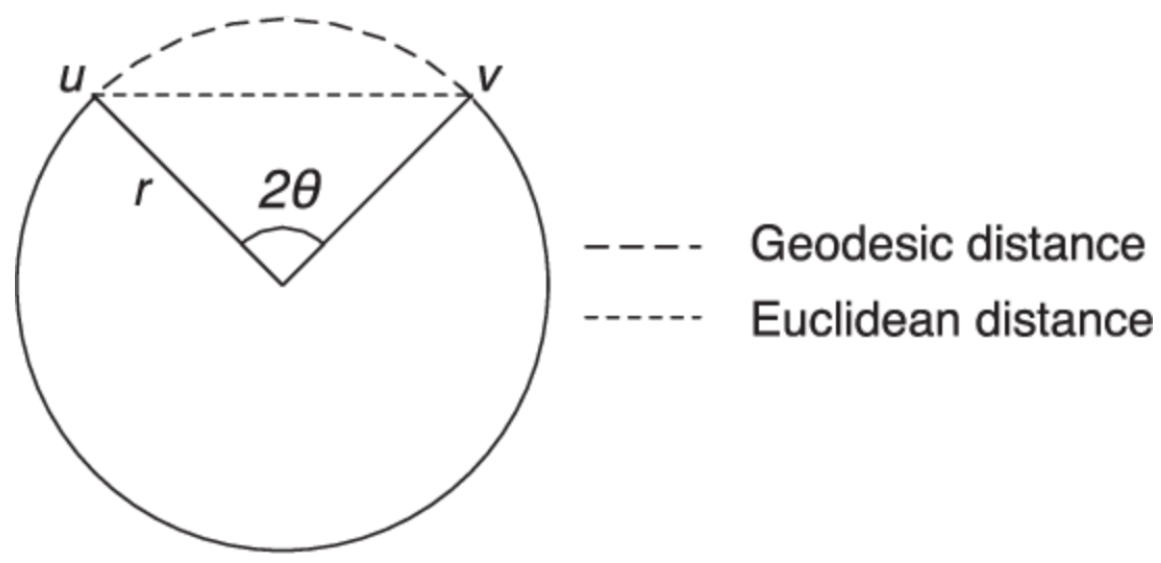
Table 1.
Notations and Definitions.
| Notation | Definition |
|---|---|
| X | Input dataset in high dimension |
| Y | Output dataset in low dimension |
| d | Original high dimension |
| k | New low dimension |
| ath input data in d dimension | |
| bth input data in d dimension | |
| ath output data in k dimension | |
| bth output data in k dimension | |
| K | Kernel function |
| c | Nearest neighbors for a data point |
| n | Number of data points |
| i | Number of iterations |
Table 2.
Development and applications of MDS, Isomap, and LLE.
| Method | Development | Applications |
|---|---|---|
| Multidimensional Scaling (MDS) | - First introduced in the 1950s. - Classical MDS formalized by Torgerson (1952). - Non-metric MDS developed by Kruskal (1964). - Widely used for dimensionality reduction in psychology, biology, and social sciences. | - Visualizing high-dimensional data in low-dimensional space. - Analyzing similarity or dissimilarity data (e.g., in marketing, linguistics [47,48,49]). - Applications in genomics for clustering gene expression data [27]. |
| Isomap | - Proposed by Tenenbaum, de Silva, and Langford (2000). - Extends classical MDS by preserving geodesic distances. - Combines ideas from graph theory and nonlinear dimensionality reduction. | - Image recognition and video synthesis [50,51,52,53]. - Face recognition and pose estimation [54,55,56,57]. - Traffic prediction [58]. - Visualizing non-linear manifolds in physics and biology [59,60,61]. |
| Locally Linear Embedding (LLE) | - Introduced by Roweis and Saul (2000). - Focuses on preserving local neighborhood relationships. - Non-parametric approach, avoids explicitly computing distances. | - Manifold learning for image and audio processing [53,62,63,64]. - Biomedical engineering such as fMRI selection [65,66].- Human activity recognition and analysis [67,68]. - Robotics for motion extraction, correction, planning and control [69,70,71,72]. |
Table 3.
Summary of Datasets
| Dataset | Type | Description | Details |
|---|---|---|---|
| SwissRoll [73] | Synthetic | Points arranged in a 3D spiral but lie on a 2D manifold | Spiral shape, 3D data |
| Iris [6] | Real | Contains 150 samples of iris flowers with 3 species | 4 features: sepal length, sepal width, petal length, petal width |
| AutoMPG [74] | Real, Regression | Predicts miles per gallon (mpg) based on car attributes | 398 samples, 9 features (e.g., cylinders, displacement) |
| MNIST [75] | Real, Image Classification, Deep Learning | 70,000 grayscale images of handwritten digits | 28x28 pixel images, digits 0-9 |
Table 5.
Complexity Comparison of MDS, Isomap, and LLE.
| Tuning of Parameters | Computational Complexity | Weakness | Transformation | |
|---|---|---|---|---|
| MDS | No. of components and iterations | Require high computation and memory to calculate dissimilarity matrix |
Dissimilarity matrix by Euclidean distance |
|
| Isomap | No. of components and nearest neighbors |
|
Suffer from topological instability |
Neighborhood graph, geodesic distance |
| LLE | No. of components, iterations and nearest neighbors |
|
Consume memory | Neighborhood graph, reconstruction weights |
Disclaimer/Publisher’s Note: The statements, opinions and data contained in all publications are solely those of the individual author(s) and contributor(s) and not of MDPI and/or the editor(s). MDPI and/or the editor(s) disclaim responsibility for any injury to people or property resulting from any ideas, methods, instructions or products referred to in the content. |
© 2025 by the authors. Licensee MDPI, Basel, Switzerland. This article is an open access article distributed under the terms and conditions of the Creative Commons Attribution (CC BY) license (http://creativecommons.org/licenses/by/4.0/).
Copyright: This open access article is published under a Creative Commons CC BY 4.0 license, which permit the free download, distribution, and reuse, provided that the author and preprint are cited in any reuse.


